Image scaling by de la Vallée-Poussin filtered interpolation

Abstract

We present a new image scaling method both for downscaling and upscaling, running with any scale factor or desired size. The resized image is achieved by sampling a bivariate polynomial which globally interpolates the data at the new scale. The method’s particularities lay in both the sampling model and the interpolation polynomial we use. Rather than classical uniform grids, we consider an unusual sampling system based on Chebyshev zeros of the first kind. Such optimal distribution of nodes permits to consider near–best interpolation polynomials defined by a filter of de la Vallée Poussin type. The action ray of this filter provides an additional parameter that can be suitably regulated to improve the approximation. The method has been tested on a significant number of different image datasets. The results are evaluated in qualitative and quantitative terms and compared with other available competitive methods. The perceived quality of the resulting scaled images is such that important details are preserved, and the appearance of artifacts is low. Competitive quality measurement values, good visual quality, limited computational effort, and moderate memory demand make the method suitable for real-world applications.

1 Introduction

Image scaling aims to get the image at a different size preserving the original content as much as possible, with minor loss of quality, in two opposite ways: downscaling and upscaling. Downscaling is a compression process by which the size of the high-resolution (HR) input image is reduced to recover the low-resolution (LR) target image. Conversely, upscaling is an enhancement process in which the size of the LR input image is enlarged to regain the HR target image.

Image scaling (also termed image resampling or image resizing) is a widely used tool in several fields such as medical imaging, remote sensing, gaming, electronic publishing, autonomous driving, and aerial photography Atkinson ; Meijering ; App1 ; App2 ; App3 ; App4 . For example, upscaling allows highlighting of important details of the image in remote sensing and medical applications Atkinson ; Meijering , while downscaling is a fundamental operation for fast browsing or sharing purposes App1 ; App2 . Other applicative examples regard scenarios like deforestation, monitoring, traffic, surveillance, and many other engineering tasks. Sometimes image scaling is used for illicit purposes, e.g., to automatically generate camouflage images whose visual semantics change dramatically after scaling Xiao . In these cases, it is very important to detect the scaling effects in order to defend against such attacks and adopt suitable countermeasures Lin ; Bruni .

From a computational point of view, image scaling can be addressed by different numerical methods (see Section 2), whose main critical points typically are: a) undesired effects, such as ringing artifacts and aliasing, due to the increase/decrease in the number of pixels which introduces/reduces information to the image; b) computational efficiency in performing the resampling task in real-world applications. Moreover, most existing methods treat the resampling in only one direction since downscaling and upscaling are often considered separate problems in literature scaling1 .

We aim to propose a scaling method that works in both downscaling and upscaling directions. To this aim, looking at the scaling problem as an approximation problem, we employ an interpolation polynomial based on an adjustable filter of de la Vallée Poussin (briefly VP) type, which can be suitably modulated to improve the approximation (see, e.g., Them_Van_Barel ; Occo_Them_LNCS ; Themistoclakis_2011 ).

Indeed, the VP type interpolation has been introduced in literature as a valid alternative to Lagrange interpolation to provide a better pointwise approximation, especially when the Gibbs phenomenon occurs Occo_Them_LNCS ; Occo_Them_AMC ; Occo_Them_Apnum . In fact, an interesting feature of VP filtered approximation is the presence of a free additional degree–parameter, which is responsible for the localization degree of the polynomial interpolation basis (the so–called fundamental VP polynomials) around the nodes. By changing this parameter, we may modulate the typical oscillatory behavior of the fundamental Lagrange polynomials according to the data, improving the approximation without destroying the interpolation property and keeping fixed the number of the interpolation nodes. Moreover, it is also worth noting that VP interpolation can be embedded in a wavelet scheme with decomposition and reconstruction algorithms very fast since based on fast cosine transforms CaThwave .

From a theoretical point of view, the literature concerning VP filtered approximation provides many convergence theorems, also in the uniform norm. They estimate an error comparable with the error of the best polynomial approximation Themistoclakis_2011 ; WoulaL1 and allow to predict the convergence order from the regularity of the function to approximate Occo_Them_DRNA . Due to such nice behavior, VP approximation has been usefully applied as a demonstration tool to carry out proofs of different theorems mastrorussothem ; Them_gauss ; Mastro_them_acta ; OccoRusso2011 ; prandtl_occo_db .

From a more applicative point of view, it has been used to solve singular integral and integro-differential equations Air_ThMastro , Prandtl_nostra or derive good quadrature rules for the finite Hilbert transform Hilbert_MG ; Hilbert_MG2 . However, to our knowledge, it has never been applied to Image Processing. Hence, the present paper represents the first step in investigating how the VP interpolation scheme can be usefully employed in image scaling.

To explain the proposed scaling method (shortly denoted by VPI method or simply by VPI), as a starting point, we consider that the input RGB image is represented at a continuous scale by a vectorial function (with separate channels for each color) whose sampling yields the pixels values. We globally approximate such function using suitable VP interpolation polynomials, modulated by a free parameter $\theta\in]0,1]$ Themistoclakis_2011 ; Them_Van_Barel ; Occo_Them_DRNA ; Occo_Them_Apnum ; Occo_Them_AMC . Hence, we get the resized image by evaluating such VP polynomials in a denser (upscaling) or coarser (downscaling) grid of sampling points.

Being designed both for downscaling and upscaling, VPI method is flexible and implementable for any scale factor. The rescaling can be obtained by specifying the scale factor or, alternatively, the desired size of the image. We point out that, in the following, to distinguish between upscaling and downscaling mode, we use the notation u-VPI and d-VPI, respectively.

Both in upscaling and downscaling, for the limiting parameter choice $\theta=0$, VPI coincides with the LCI method proposed in Lagrange and based on classical Lagrange interpolation at the same nodes. Moreover, for any choice of the parameter $\theta$, d-VPI with odd scale factors also produces the same output resized image of LCI, which results by a direct assignment without any computation. In these cases, if the LR image satisfies the Nyquist-Shannon sampling theorem Shannon , d-VPI produces a MSE not greater than input MSE times the scale factor squared. Thus, we can get a null MSE and the best visual quality measures in case of exact input data (cf. Proposition 1). However, we point out that in cases where the downscaling size violates the sampling theorem, aliasing effects occur. Experiments in the paper also deepen this aspect, and a partial solution is proposed, remaining the problem open to further investigations.

A further contribution of this paper includes a detailed quantitative and qualitative analysis of the obtained results on several publicly available datasets commonly used in Image Processing. The experimental results confirm the effectiveness and utility of employing the VP interpolation scheme, achieving on average a good compromise between visual quality and processing time: the resized images present few blurred edges and artifacts, and the implementation is computationally simple and rather fast.

On average, VPI has a competitive and satisfactory performance, with quality measures generally higher and more stable than other existing scaling methods considered as a benchmark. In general, we have satisfactory performance, also for high scale factors, compared to the benchmark methods. Specifically, in downscaling, when the free parameter is not equal to zero, VPI improves the LCI performance and results to be more stable than the latter due to the uniform boundedness of Lebesgue constants corresponding to the de la Vallée Poussin type interpolation. Moreover, VPI results much faster than the methods specialized in only downscaling or upscaling.

At a visual level, VPI captures the object’s visual structure by preserving the salient details, the local contrast, and the luminance of the input image, with well–balanced colors and a limited presence of artifacts. To about the same extent as the other benchmark methods, in downscaling VPI exhibits aliasing effects.

Overall, due to its features, we consider VPI suitable for real–world applications, and, at the same time, we look at it as a complete method because it can also perform upscaling and downscaling with adequate performance.

The remainder of this paper is as follows. In Section 2, we outline the related work, briefly explaining the benchmark scaling methods we employ in the experimental phase. In Section 3 we provide the mathematical background. In Section 4, we describe the VPI method and state its main properties. In Section 5 we provide the most relevant implementation details and the qualitative/quantitative evaluations of the experimental results taken over a significant numebr of different image datasets. Finally, conclusions are drawn in Section 6.

2 Related work

Image scaling has received great attention in the literature of the past decades, during which many methods based on different approaches have been developed. An overview containing pros and cons for some of them can be found in rev1 ; rev2 .

Traditionally, image scaling methods are grouped into two categories book1 : non-adaptive NN-NIL2 ; Lanczos ; B-splines ; Burger ; ScSR and adaptive Stentiford ; Setlur ; Ramella2 ; Zhou ; Yang . In the first category, all the pixels are equally treated. In the second, suitable changes are arranged, depending on image features and intensity values, edge information, texture, etc. The non-adaptive category includes many of the most commonly used algorithms such as the nearest neighbor, bilinear, bicubic and B-splines interpolation, Lanczos method book1 ; NN-NIL2 ; Lanczos ; B-splines ; Burger ; CN . Adaptive methods are designed to maximize the quality of the results. They are also employed in most common approaches such as context-aware computing Stentiford , segmentation techniquesSetlur , and adaptive bilinear schemes Ramella2 . Machine Learning (ML) methods can be ascribed to the latter category,even if they are often considered as a separate problem Zhou ; Yang . The learning paradigm of ML methods aims to compensate for complete (missing) information of the downscaled (upscaled) image using a relationship between HR (LR) and LR (HR) images. Mostly, this paradigm is implemented by a training step, in which the relationship is learned, followed by a step in which the learned knowledge is applied to unseen HR (LR) images.

Usually, non-adaptive scaling methods have problems of blurring or artifacts around edges and only store the low-frequency components of the original image. On the other hand, adaptive scaling methods generally provide better image visual quality and preserve high-frequency components. However, adaptive methods take more computational time as compared to non-adaptive ones. In turn, the ML methods ensure high-quality results but, at the same time, require extensive learning based on a huge number of parameters and labeled training images.

In this section, we limit to describe shortly the methods considered in the validation phase of the VPI method (see Section 5), namely DPID Weber , L₀ Liu , SCN SCN , LCI Lagrange and BIC BIC . The source code of such methods is made available by the authors themselves in a common language (Matlab). Except for BIC and LCI, these methods are designed and tested considering the problem of resizing in one direction, i.e., in downscaling (DPID and L₀) or upscaling mode (SCN).

DPID is based on the assumption that the Laplacian edge detector and adaptive low-pass filtering can be useful tools to approximate the behavior of the Human Visual System. Important details are preserved in the downscaled image by employing convolutional filters and by selecting the input pixels that contribute more to the output image the more their color deviates from their local neighborhood.

In L₀, an optimization framework for image downscaling, focusing on two critical issues, is proposed: salient features preservation and downscaled image construction. Accordingly, two L₀-regularized priors are introduced and applied iteratively until the objective function is verified. The first, based on gradient ratio, allows preserving the most salient edges and the visual perceptual properties of the original image. The second optimates the downscaled image by the guidance of the original one, avoiding undesirable artifacts.

SCN (Sparse Coding based Network) adopts a neural network based on sparse coding, trained in a cascaded structure from end to end. It introduces some improvements in terms of both recovery accuracy and human perception employing a CNN (Convolutional Neural Network) model.

In LCI, the input RGB image is globally approximated by the bivariate Lagrange interpolating polynomial at a suitable grid of first kind Chebyshev zeros. The output RGB image is obtained by sampling this polynomial at the Chebyshev grid of the desired size. Since the LCI method works both in upscaling and downscaling, according to the notation in Lagrange , we use the notation u-LCI and d-LCI in upscaling and in downscaling, respectively.

BIC, one of the most commonly used rescaling methods, employs bicubic interpolation. It computes the unknown pixel value as a weighted average of $4\times 4$ pixels closest to it. Note that BIC produces noticeably sharper images than the other classical non-adaptive methods such as bilinear and nearest neighbor, offering w.r.t. them a favorable quality image and processing time ratio.

We remark that in the following, BIC is implemented by the Matlab built-in function imresize with bicubic option. For the other methods, we used the publicly available Matlab codes provided by the authors with the default parameters settings.

3 Mathematical preliminaries

Let $I$ denote any color image of $n_{1}\times n_{2}$ pixels, with $n_{1},n_{2}\in{\mathbb{N}}$. As is well–known, in the RGB space $I$ is represented by means of a triad of $n_{1}\times n_{2}$ matrices that we indicate using the same letter of the image they compose, namely $I_{\lambda}$, with $\lambda=1:3$ (i.e., $\lambda=1,2,3$). The entries of these matrices are integers from $0$ to $\max_{f}$ that denotes the maximum possible value of the image pixel, (e.g., $\max_{f}=255$ if the pixels are represented using 8 bits per sample). On the other hand, such discrete values can be embedded in a vector function of the spatial coordinates, say ${\mathbf{f}}(x,y)=[f_{1}(x,y),f_{2}(x,y),f_{3}(x,y)]$, which represents the image at a continuous scale and whose sampling yields its digital versions of any finite size.

Hence, once fixed the sampling model, that is the system of nodes

$$X_{\mu\times\nu}=\{(x_{i}^{\mu},y_{j}^{\nu})\}_{i=1:\mu,j=1:\nu},\quad\mu,\nu\in{\mathbb{N}},$$ (1)

we suppose that the digital image $I=[I_{1},I_{2},I_{3}]$ has behind the function ${\mathbf{f}}=[f_{1},f_{2},f_{3}]$ such that

$$I(i,j)={\mathbf{f}}(x_{i}^{n_{1}},y_{j}^{n_{2}}),\quad i=1:n_{1},\quad j=1:n_{2}.$$ (2)

In both downscaling and upscaling, the goal is getting an accurate reconstruction of $I$ at a different (reduced and enhanced, resp.) size. Denoting by $N_{1}\times N_{2}$ the new size that we aim to get and denoting by $R=[R_{1},R_{2},R_{3}]$ the target resized image of $N_{1}\times N_{2}$ pixels, according to the previous settings, we have

$$R(i,j)={\mathbf{f}}(x_{i}^{N_{1}},y_{j}^{N_{2}}),\quad i=1:N_{1},\quad j=1:N_{2}.$$ (3)

From this viewpoint, the scaling problem becomes a typical approximation problem: how to approximate the values of ${\mathbf{f}}$ at the grid $X_{N_{1}\times N_{2}}$ once known the values of ${\mathbf{f}}$ at the finer (in downscaling) or coarser (in upscaling) grid $X_{n_{1}\times n_{2}}$.

Within this setting, the choice of the nodes system (1) as well as the choice of the approximation tool are both decisive for the success of a scaling method. In the next subsections we introduce these two basic ingredients and the evaluation metrics we use for our scaling method.

3.1 Sampling system

Since it is well–known that any finite interval $[a,b]$ can be mapped onto $[-1,1]$, in the following, we suppose that each spatial coordinate belongs to the reference interval $[-1,1]$, so that the sampling system in (1) is included in the square $[-1,1]^{2}$.

In literature, the equidistant nodes model is usually adopted for sampling. According to such traditional model, in (1) the coordinates $\{x_{i}^{\mu}\}_{i}$ and $\{y_{j}^{\nu}\}_{j}$ are those nodes that divide the segment $[-1,1]$ into $(\mu+1)$ and $(\nu+1)$ equal parts, respectively. On the other hand, we recall that other coherent choices of the sampling system (1) have been recently investigated, for instance, in demarchi1 , demarchi2 for Magnetic Particle Imaging.

Here we follow the sampling model recently introduced in Lagrange . According to this model, we assume that (1) is the Chebyshev grid where the coordinates $\{x_{i}^{\mu}\}_{i}$ and $\{y_{j}^{\nu}\}_{j}$ are the zeros of the Chebyshev polynomial of first kind of degree $\mu$ and $\nu$, respectively. This means that in (1) we are going to assume that

$$x_{i}^{\mu}=\cos(t_{i}^{\mu})\qquad\mbox{and}\qquad y_{j}^{\nu}=\cos(t_{j}^{\nu})$$ (4)

where, for all $n\in{\mathbb{N}}$, it is

$$t_{k}^{n}=\frac{(2k-1)\pi}{2n},\qquad k=1:n.$$ (5)

Hence, supposed that ${\mathbf{f}}$ is the vector function representing the image at a continuous scale, at a discrete scale we interpret the digital version of the image with size $\mu\times\nu$, as resulting from the sampling of ${\mathbf{f}}$ at the Chebyshev grid $X_{\mu\times\nu}$ defined by (1) and (4)-(5).

We point out that both the coordinates in (4) are not equidistant in $[-1,1],$ but they are arcsine distributed and become denser approaching the extremes $\pm 1$. Such nodes distribution is optimal from the approximation point of view but rather unusual in image sampling. Nevertheless, from a certain perspective, our sampling model is related to the traditional sampling at equidistant nodes since the nodes in (5) are equally spaced in $[0,\pi]$. Indeed, the idea behind our sampling model is to transfer the sampling question from the segment to the unit semicircle, which is divided into equal arcs by the nodes system equation (5).

The main advantage of adopting this unusual point of view is the possibility of globally approximating the image, in a stable and near–best way, by the interpolation polynomials introduced in the next subsection.

3.2 Filtered VP interpolation

Regarding the approximation tool underlying our method, we consider some filtered interpolation polynomials recently studied in Occo_Them_AMC . Such kind of interpolation is based on a generalization of the trigonometric VP means (see Filbir_Them ; Them_Van_Barel ) and, besides the number of nodes, it depends on two additional parameters which can be suitable modulated in order to reduce the Gibbs phenomenon (see Occo_Them_AMC ; Themistoclakis_2011 ).

More precisely, for any $n_{i},m_{i}\in{\mathbb{N}}$ such that $m_{i}\leq n_{i}$, $i=1,2$, let

$${\mathbf{n}}=(n_{1},n_{2}),\quad\mbox{and}\quad{\mathbf{m}}=(m_{1},m_{2}),$$

and let $n,m$ denote indifferently the first components (i.e. $n_{1},m_{1}$ resp.) or the second components (i.e. $n_{2},m_{2}$ resp.) of such vectors. Corresponding to these parameters, for any $r=0:(n-1)$, we define the following orthogonal VP polynomials

$$q_{m,r}^{n}(\xi)=\left\{\begin{array}[]{l}\cos(rt)\qquad\qquad\mbox{if $0\leq r\leq(n-m)$},\\[7.22743pt] \frac{n+m-r}{2m}\cos(rt)+\frac{n-m-r}{2m}\cos((2n-r)t)\\[5.05942pt] \qquad\qquad\qquad\mbox{if $n-m<r<n$},\end{array}\right.$$ (6)

where here and in the following $\xi\in[-1,1]$ and $t\in[0,\pi]$ are related by $\xi=\cos t$.

We recall the polynomial system in (6) consists of $n$ univariate algebraic polynomials of degree at most $(n+m-1)$ that are orthogonal with respect to the scalar product

$$<F,G>=\int_{-1}^{1}F(\xi)G(\xi)\frac{d\xi}{\sqrt{1-\xi^{2}}}.$$

They generate the space (of dimension $n$)

$$S_{m}^{n}:=\textrm{span}\{q_{m,r}^{n}:\ r=0:(n-1)\}$$

that is an intermediate polynomial space nested between the sets of all polynomials of degree at most $n-m$ and $n+m-1$.

The space $S_{m}^{n}$ has also an interpolating basis consisting of the so–called fundamental VP polynomials that, in terms of the orthogonal basis (6), have the following expansion Themistoclakis_2011 ,Occo_Them_AMC

$$\Phi_{m,k}^{n}(\xi)=\frac{2}{n}\left[\frac{1}{2}+\sum_{r=1}^{n-1}\cos(rt_{k}^{n})q_{m,r}^{n}(\xi)\right],\quad k=1:n.$$ (7)

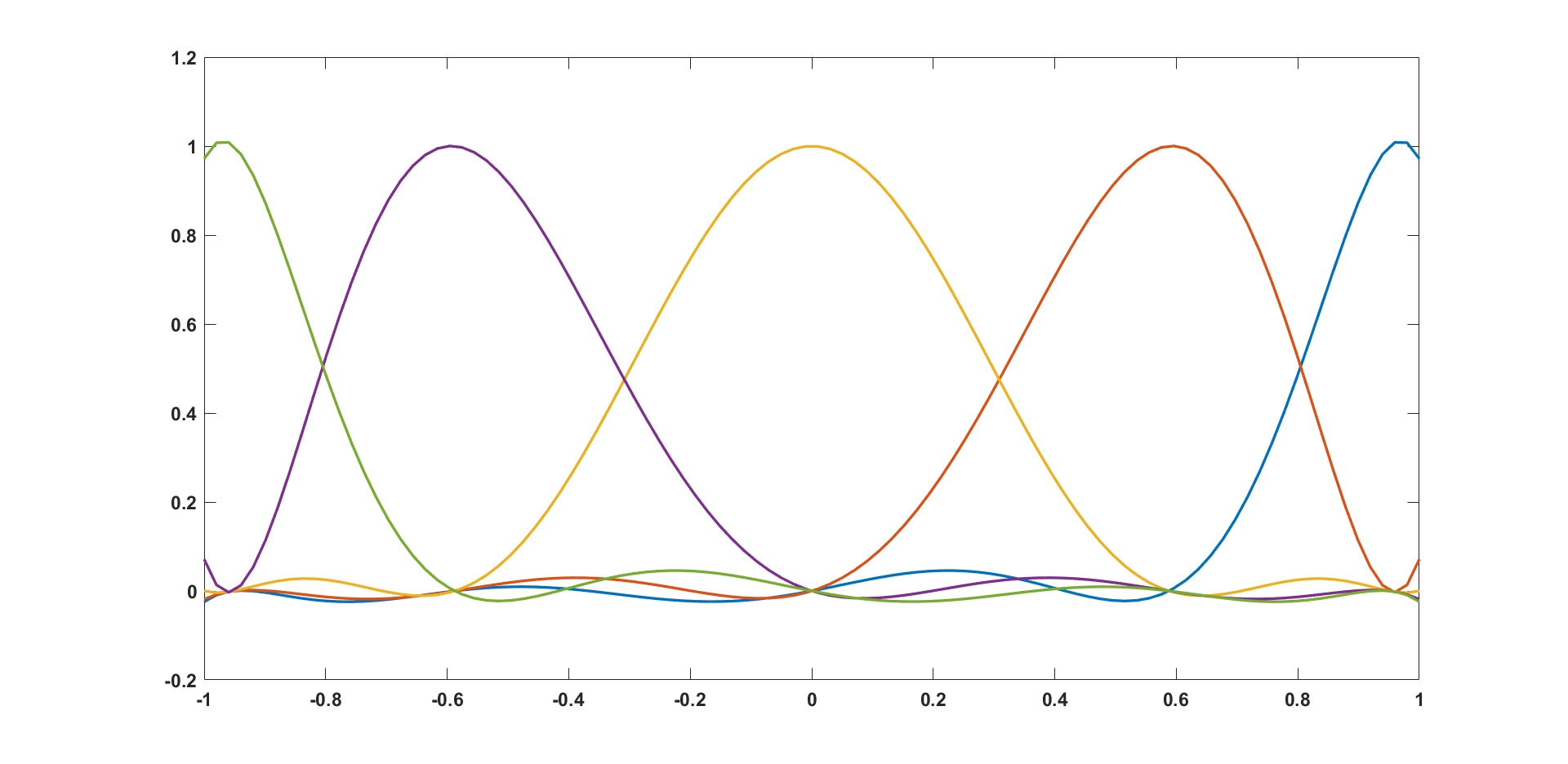
Figure 1: Fundamental VP polynomials $\{\Phi_{m,k}^{n}\}_{k=1}^{n}$ for $n=5$ and $m=4$

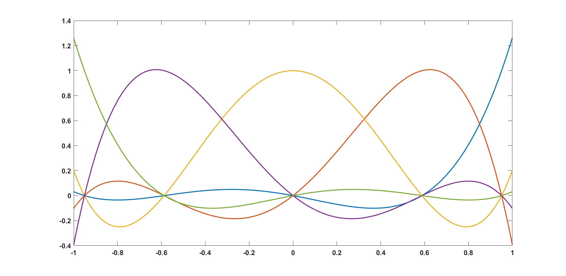
Figure 2: Fundamental Lagrange polynomials $\{\ell_{n,k}\}_{k=1}^{n}$ for $n=5$

In Figures 1 and 2 we show respectively the fundamental VP polynomials for $n=5$ and $m=4$, and for the same $n=5$, the well-known fundamental Lagrange polynomials, defined as

$$l_{n,k}(\xi)=\frac{2}{n}\left[\frac{1}{2}+\sum_{r=1}^{n-1}\cos(rt_{k}^{n})\cos(rt)\right],\quad k=1:n.$$ (8)

We see that, similarly to $\{l_{n,k}(\xi)\}_{k=1}^{n}$ also the fundamental VP polynomials satisfy the interpolation property

$$\Phi_{m,k}^{n}(\cos t_{h}^{n})=l_{n,k}(\cos t_{h}^{n})=\left\{\begin{array}[]{lr}1&h=k\\ 0&h\neq k\end{array}\right.$$ (9)

for all $h,k=1:n$.

In addition to the number $n$ of nodes, we also have the free parameter $m$ which can be arbitrarily chosen ($m=1:n$ being possible) without loosing the interpolation property (9), as stated in Themistoclakis_2011 . Moreover, we note that also the limiting choice $m=0$ is possible, being, in this case, $S_{0}^{n}$ equal to the space of polynomials of degree at most $(n-1)$ and

$$\Phi_{0,k}^{n}(\xi)=l_{n,k}(\xi),\qquad\forall|\xi|\leq 1,\qquad k=1:n.$$ (10)

We recall in CaThwave both $n,m$ are chosen depending on a resolution level $\ell\in{\mathbb{N}}$ and the fundamental VP polynomials constitute the scaling functions generating the multiresolution spaces $V_{\ell}=S_{m}^{n}$.

Another choice of $m$, often suggested in literature, is the following (see e.g. Occo_Them_Apnum ,Occo_Them_DRNA )

$$m=\lfloor\theta n\rfloor,\qquad\mbox{with $\theta\in]0,1[$},$$ (11)

where, $\forall a\in{\mathbb{R}}^{+}$, $\lfloor a\rfloor$ denotes the largest integer not greater than $a$.

Figure 3 displays the plots of the fundamental VP polynomials corresponding to fixed $n,k$ and $m$ given by (11) with different values of $\theta$. Indeed such parameter (and more generally $m$) is responsible for the localization of the fundamental VP polynomial $\Phi_{n,k}^{m}(\xi)$ around the node $\xi_{k}^{n}=\cos t_{k}^{n}$. In fact, in Figure 3 we can see how those oscillations typical of the fundamental Lagrange polynomial $\ell_{n,k}$ (plotted too) are very dampened by suitable choices of $\theta$.

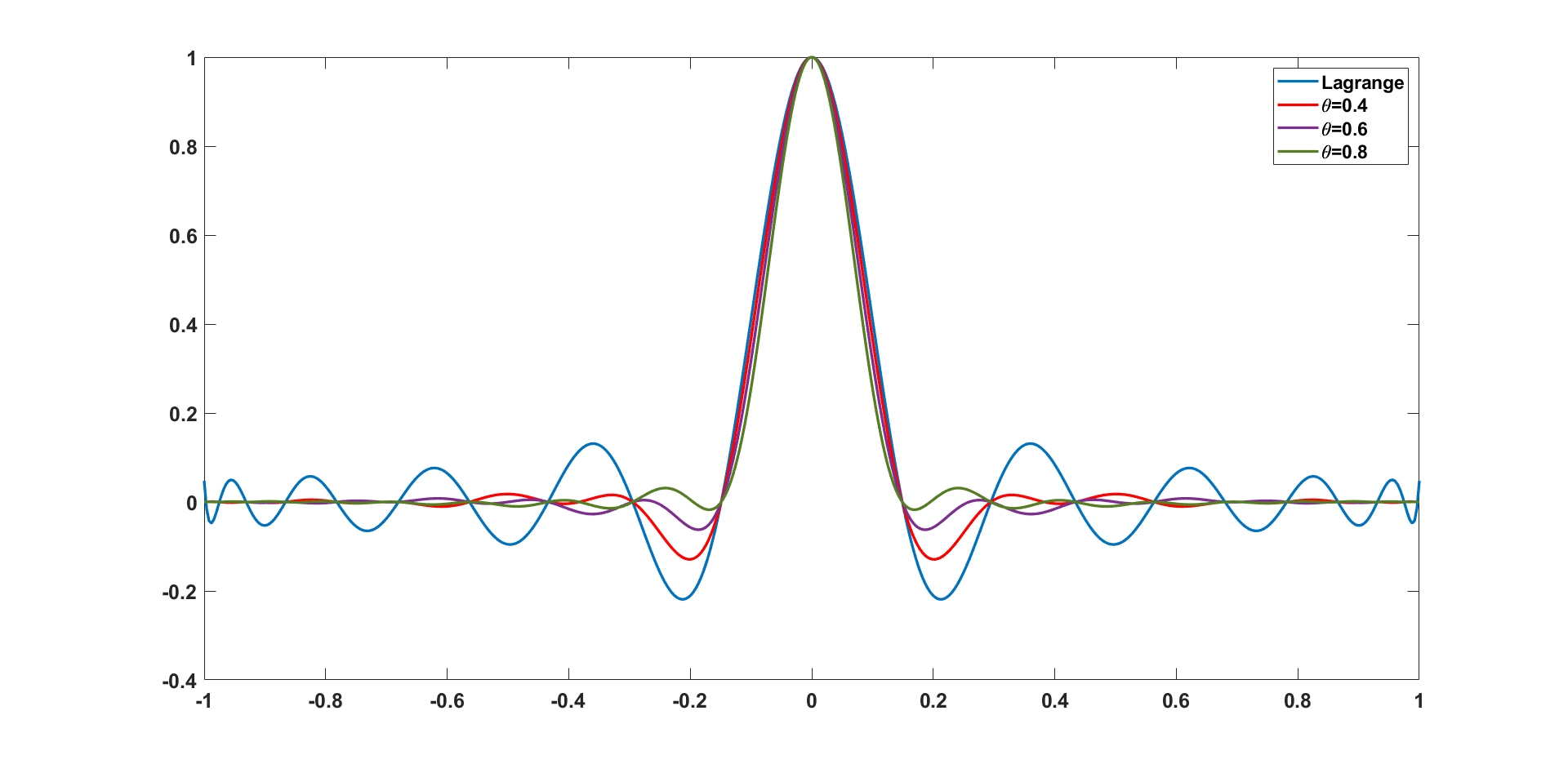
Figure 3: Fundamental polynomials $\ell_{n,k}$ and $\Phi_{m,k}^{n}$ for $n=21,\ k=11$ and $m=\lfloor n\theta\rfloor,$ with $\theta\in\{\ 0.4,\ 0.6,\ 0.8\}.$

By using the fundamental VP polynomials (7) we can approximate any function $g(x,y)$ on the square $[-1,1]^{2}$ by means of its samples at the Chebyshev grid (1) as follows

$$V_{{\mathbf{n}}}^{{\mathbf{m}}}g(x,y):=\sum_{i=1}^{n_{1}}\sum_{j=1}^{n_{2}}g(x_{i}^{n_{1}},y_{j}^{n_{2}})\Phi_{n_{1},i}^{m_{1}}(x)\Phi_{n_{2},j}^{m_{2}}(y).$$ (12)

This is the definition of the VP polynomial of $g$ and the approximation tool we use in our method.

By virtue of (9), such polynomial coincides with $g$ at the grid $X_{n_{1}\times n_{2}}$, i.e.

$$V_{{\mathbf{n}}}^{{\mathbf{m}}}g(x_{i}^{n_{1}},y_{j}^{n_{2}})=g(x_{i}^{n_{1}},y_{j}^{n_{2}}),\quad i=1:n_{1},\ j=1:n_{2},$$ (13)

Moreover, it has been proved that for any $(x,y)\in[-1,1]^{2}$, if (26) holds with an arbitrarily fixed $\theta\in]0,1[$ then for all continuous functions $g$, the following limit holds uniformly on $[-1,1]^{2}$

$$\lim_{{\mathbf{n}}\rightarrow\infty}\left|V_{{\mathbf{n}}}^{{\mathbf{m}}}g(x,y)-g(x,y)\right|=0$$

with the same convergence rate of the error of best polynomial approximation of $g$ (Occo_Them_AMC, , Th.3.1).

3.3 Quality metrics

Similar to most of the existing methods in literature, the performance of our method is quantitatively evaluated and compared with other scaling methods in terms of the Peak-Signal-to-Noise-Ratio (PSNR) and the Structural Similarity Index (SSIM). For our method such metrics will give a measure of the error between the target resized image $R=[R_{1},R_{2},R_{3}]$ and the output resized image that, in the following, we denote by $\tilde{R}=[\tilde{R}_{1},\tilde{R}_{2},\tilde{R}_{3}]$ .

The definition of PSNR is based on the standard definition of the Mean Squared Error between two matrices

$$\rm{MSE}(A,B)=\displaystyle\frac{1}{\nu\mu}\|A-B\|_{F}^{2},\qquad\forall A,B\in{\mathbb{R}}^{\nu\times\mu}$$ (14)

being $\|\cdot\|_{F}$ the Frobenius norm defined as

$$\|A\|_{F}:=\left(\sum_{h=1}^{\nu}\sum_{k=1}^{\mu}a_{h,k}^{2}\right)^{\frac{1}{2}},\ \forall A=(a_{h,k})\in{\mathbb{R}}^{\nu\times\mu}.$$

The extension of such definition to the case of color digital images of $\nu\times\mu$ pixels can be performed in different ways giving rise to different measures of the related PSNR (see e.g. Ramella1 ; Matlab ). More precisely, for the color images $R$ and $\tilde{R}$, defining their MSE as follows

$$\rm{MSE}(\tilde{R},R)=\frac{1}{3}\sum_{\lambda=1}^{3}\rm{MSE}(\tilde{R}_{\lambda},R_{\lambda}),$$ (15)

the first, usually adopted definition of PSNR (used for instance in Lagrange ) is the following

$$\rm{PSNR}(\tilde{R},R)=20\log_{10}\left(\frac{\max_{f}}{\sqrt{\rm{MSE}(\tilde{R},R)}}\right).$$ (16)

Another common way to measure the PSNR (also used in SCN ) is given by converting to the color space YCrCb both the color RGB images $R=[R_{1},R_{2},R_{3}]$ and $\tilde{R}=[\tilde{R}_{1},\tilde{R}_{2},\tilde{R}_{3}]$, and separating the intensity Y (luma) channels that we denote by $R_{Y}$ and $\tilde{R}_{Y}$, respectively. We recall they are defined by the following weighted average of the respective RGB components

$$R_{Y}=\sum_{\lambda=1}^{3}\alpha_{\lambda}R_{\lambda}+\alpha_{4},\quad\tilde{R}_{Y}=\sum_{\lambda=1}^{3}\alpha_{\lambda}\tilde{R}_{\lambda}+\alpha_{4},$$ (17)

with $\alpha_{i},\ i=1:4$ coefficients of the ITU -R BT.601 standard (see e.g. Burger ). Hence, taking the MSE of the matrices $R_{Y}$ and $\tilde{R}_{Y}$, the second, commonly used, definition of PSNR is referred to only such luma channel as follows

$$\rm{PSNR}(\tilde{R},R)=20\displaystyle\log_{10}\left(\frac{\max_{f}}{\sqrt{\rm{MSE}(\tilde{R}_{Y},R_{Y})}}\right),$$ (18)

We point out that in our experiments the PSNR has been computed using both the previous definitions. However, for brevity, in this paper we report only the values achieved by definition (18), giving no new insight the results obtained by using the other definition (16).

Finally, also the SSIM metric is defined via the luma channel as follows SSIM

$$\rm{SSIM}(\tilde{R},R)=\frac{\left[2\tilde{\mu}\mu+c_{1}\right]\left[2\rm{cov}+c_{2}\right]}{\left[{\tilde{\mu}}^{2}+\mu^{2}+c_{1}\right]\left[{\tilde{\sigma}}^{2}+\sigma^{2}+c_{2}\right]},$$ (19)

where $\tilde{\mu},\mu$ and $\tilde{\sigma},\sigma$ denote the average and variance of the matrices $\tilde{R}_{Y},R_{Y}$, respectively, $\rm{cov}$ indicates their covariance, and the constants are usually fixed as $c_{1}=(0.01\times L),c_{2}=(0.03\times L)$ with the dynamic range of the pixel values $L=255$ in the case of 8-bit images.

4 VPI scaling method

According to the notation introduced in the previous section, both $I$ and $R$ are digital versions (with $n_{1}\times n_{2}$ and $N_{1}\times N_{2}$ pixels, respectively) of the same continuous image represented by the vector function ${\mathbf{f}}=(f_{1},f_{2},f_{3})$ (cf. (2), (3)). Nevertheless, to be more general, in view of the finite representation of the data and the accuracy used to store the image, we suppose the effective input image of our method is a more or less corrupted version of $I$. We denote it by $\tilde{I}=[\tilde{I}_{1},\tilde{I}_{1},\tilde{I}_{3}]$ and assume that there exists a corrupted function $\widetilde{\mathbf{f}}=(\widetilde{f}_{1},\widetilde{f}_{2},\widetilde{f}_{3})$ such that

$$\tilde{I}(i,j)=\tilde{\mathbf{f}}(x_{i}^{n_{1}},y_{j}^{n_{2}}),\quad i=1:n_{1},\quad j=1:n_{2}.$$ (20)

Starting from these initial data, VPI method computes the output image $\tilde{R}$ having the desired size $N_{1}\times N_{2}$ and defined as follows

$$\tilde{R}(i,j)=V_{{\mathbf{n}}}^{{\mathbf{m}}}\tilde{\mathbf{f}}(x_{i}^{N_{1}},y_{j}^{N_{2}}),\ i=1:N_{1},\ j=1:N_{2}.$$ (21)

In terms of the RGB components $\tilde{R}=[\tilde{R}_{1},\tilde{R}_{2},\tilde{R}_{3}]$, by (12), this means that for any $i=1:N_{1},\ j=1:N_{2}$ and $\lambda=1:3$ we have

$$\tilde{R}_{\lambda}(i,j) = V_{{\mathbf{n}}}^{{\mathbf{m}}}\tilde{f}_{\lambda}(x_{i}^{N_{1}},y_{j}^{N_{2}})=$$

$$= \sum_{u=1}^{n_{1}}\sum_{v=1}^{n_{2}}\tilde{I}_{\lambda}(u,v)\Phi_{n_{1},u}^{m_{1}}(x_{i}^{N_{1}})\Phi_{n_{2},v}^{m_{2}}(y_{j}^{N_{2}}),$$

that is

$$\tilde{R}_{\lambda}=V_{1}^{T}\tilde{I}_{\lambda}V_{2},\quad\lambda=1:3,$$ (23)

where the matrices $V_{1}\in{\mathbb{R}}^{n_{1}\times N_{1}}$ and $V_{2}\in{\mathbb{R}}^{n_{2}\times N_{2}}$ have the following entries

$$V_{1}(i,j) = \Phi_{n_{1},i}^{m_{1}}(x_{j}^{N_{1}}),\qquad i=1:n_{1},\ j=1:N_{1}$$ (24)

$$V_{2}(i,j) = \Phi_{n_{2},i}^{m_{2}}(y_{j}^{N_{2}}),\qquad i=1:n_{2},\ j=1:N_{2}$$ (25)

To compute $V_{1},V_{2}$ efficient algorithms based on Fast Fourier transform can be implemented (see, e.g., FFT ). Moreover, by pre-computing matrices $V_{i}$, the representation (23) allows to reduce the computational effort when we have to resize many images for the same fixed sizes.

Now, we note that in the previous formulas, the integers $n_{\ell}$ and $N_{\ell}$ for $\ell=1,2$ are determined by the initial and final size of the scaling problem at hand, while the parameter $m_{\ell}$ is free. Theoretically, it can be arbitrarily chosen from the set of integers between 1 and

$n_{\ell}$. According to (11), for our method we fix

$$m_{\ell}=\lfloor\theta n_{\ell}\rfloor,\qquad\ell=1,2,\qquad\mbox{with}\qquad\theta\in]0,1]$$ (26)

including the limit case $\theta=1$ too. Moreover, we also allow $\theta=0$, but, in this case, we remark that, by virtue of (10), VPI reduces to Lagrange–Chebyshev Interpolation (LCI) scaling method recently proposed in Lagrange . In this sense, VPI can be considered a generalization of the LCI method.

Regarding the choice of the parameter $\theta$, in the experimental validation of VPI, we consider two modes that we indicate in the sequel: ”supervised VPI” and ”unsupervised VPI”. In the latter case, $\theta$ must be supplied by the user as an input parameter, arbitrarily chosen in $[0,1]$, where the choice $\theta=0$ means to select the LCI method.

Nevertheless, if a target resized image is available, we have structured VPI method in a supervised mode that requires the target image as input argument, instead of the parameter $\theta$. In this case, we take several choices of $\theta\in[0,1]$ and, consequently, we get several matrices $V_{1},V_{2}$ that determine, using (23), several resized images. Among these images, the one that, once compared with the target image, gives the smallest MSE is chosen as the output image of the supervised VPI method.

In the sequel of this Section, we focus on d-VPI method with odd scale factors $s=n_{1}/N_{1}=n_{2}/N_{2}$. In the following proposition, we suppose that the lower resolution sampling satisfies the Nyquist limit so that the continuous image ${\mathbf{f}}$ can be uniquely reconstructed from both digital images $I$ and $R$ without any error. In this ideal case, we prove d-VPI method produces a MSE that it is not greater than $s^{2}$ times the MSE of the input data (cf. (28)) and, in particular, we get a null MSE if the input image is exact or, at least, only some crucial pixels of it are exact (cf. Remark 1).

Proposition 1

Let $I$ and $R$ be the initial and resized true images given by (2) and (3) respectively, and let $\tilde{I}$ and $\tilde{R}$ by input and output images of d-VPI method, respectively given by (20) and (21), with arbitrarily fixed integer parameters $m_{1}<n_{1}$ and $m_{2}<n_{2}$. If there exists $\ell\in{\mathbb{N}}$ that relates the initial size $n_{1}\times n_{2}$ with the final size $N_{1}\times N_{2}$ as follows

$$\frac{n_{1}}{N_{1}}=\frac{n_{2}}{N_{2}}=(2\ell-1),$$ (27)

then we have

$$\rm{MSE}(R,\tilde{R})\leq s^{2}\rm{MSE}(I,\tilde{I}),\qquad s=(2\ell-1).$$ (28)

The same estimate holds also for the luma channel and, if in addition $I=\tilde{I}$ holds too, then we get

$$\rm{PSNR}(R,\tilde{R})=\infty,\qquad\mbox{and}\qquad\rm{SSIM}(R,\tilde{R})=1.$$ (29)

Proof. Recalling the definition (15), to prove (28) it is sufficient to state the same inequality holds for the respective RGB components. Hence, according to our notation, let us state that for all $\lambda=1:3$ we have

$$\rm{MSE}(R_{\lambda},\tilde{R}_{\lambda})<s^{2}\rm{MSE}(I_{\lambda},\tilde{I}_{\lambda}).$$ (30)

To this aim, by using the short notation $n$ and $N$ to denote $n_{i}$ and $N_{i}$, respectively, for any $i=1,2$, we note that whenever we have $n=sN$ with $s=(2\ell-1)$ and $\ell\in{\mathbb{N}}$, all the zeros of the first kind Chebyshev polynomial of degree $N$ (i.e. $\cos(t_{h}^{N})$ with $h=1:N$) are also zeros of the first kind Chebyshev polynomial of degree $n$. More precisely, we have

$$\cos(t_{h}^{N})=\cos(t_{i(h)}^{n})\quad\mbox{with\ }i(h)=\frac{s(2h-1)+1}{2},$$ (31)

where we point out that for all $h=1:N$ the index $i(h)=\frac{s(2h-1)+1}{2}$ is an integer between 1 and $n$ thanks to the hypothesis $s$ is odd.

By virtue of (31), for all $h_{1}=1:N_{1}$ and $h_{2}=1:N_{2}$, recalling (3)–(5) we get

$$\begin{array}[]{rl}R_{\lambda}(h_{1},h_{2})=&f_{\lambda}\left(x_{h_{1}}^{N_{1}},y_{h_{2}}^{N_{2}}\right)\\ =&f_{\lambda}\left(x_{i(h_{1})}^{n_{1}},y_{i(h_{2})}^{n_{2}}\right)\\ =&I_{\lambda}\left(i(h_{1}),\ i(h_{2})\right),\qquad\lambda=1:3.\end{array}$$ (32)

Similarly, from (21), (31), (13) and (20), we deduce

$$\begin{array}[]{rl}\tilde{R}_{\lambda}(h_{1},h_{2})=&V_{{\mathbf{n}}}^{{\mathbf{m}}}\tilde{f}_{\lambda}\left(x_{h_{1}}^{N_{1}},y_{h_{2}}^{N_{2}}\right)\\[7.22743pt] =&V_{{\mathbf{n}}}^{{\mathbf{m}}}\tilde{f}_{\lambda}\left(x_{i(h_{1})}^{n_{1}},y_{i(h_{2})}^{n_{2}}\right)=\tilde{f}_{\lambda}\left(x_{i(h_{1})}^{n_{1}},y_{i(h_{2})}^{n_{2}}\right)\\[7.22743pt] =&\tilde{I}_{\lambda}\left(i(h_{1}),\ i(h_{2})\right),\qquad\lambda=1:3.\end{array}$$ (33)

Therefore, by (32) and (33), for any $\lambda=1:3$ we deduce (30) as follows

$$\rm{MSE}(R_{\lambda},\tilde{R}_{\lambda})=$$

$$= \frac{1}{N_{1}N_{2}}\sum_{h_{1}=1}^{N_{1}}\sum_{h_{2}=1}^{N_{2}}\left[R_{\lambda}(h_{1},h_{2})-\tilde{R}_{\lambda}(h_{1},h_{2})\right]^{2}$$

$$= \frac{1}{N_{1}N_{2}}\sum_{h_{1}=1}^{N_{1}}\sum_{h_{2}=1}^{N_{2}}\left[I_{\lambda}\left(i(h_{1}),\ i(h_{2})\right)-\tilde{I}_{\lambda}\left(i(h_{1}),\ i(h_{2})\right)\right]^{2}$$

$$\leq \frac{1}{N_{1}N_{2}}\sum_{i=1}^{n_{1}}\sum_{j=1}^{n_{2}}\left[I_{\lambda}(i,j)-\tilde{I}_{\lambda}(i,j))\right]^{2}$$

$$= \frac{s^{2}}{n_{1}n_{2}}\sum_{i=1}^{n_{1}}\sum_{j=1}^{n_{2}}\left[I_{\lambda}(i,j)-\tilde{I}_{\lambda}(i,j))\right]^{2}$$

$$= s^{2}\rm{MSE}(I_{\lambda},\tilde{I}_{\lambda}).$$

As regards the luma chanel, we note that by (32)–(33) and (17) we easily deduce that

$$\begin{array}[]{rl}R_{Y}(h_{1},h_{2})=&I_{Y}(i(h_{1}),\ i(h_{2}))\\ \tilde{R}_{Y}(h_{1},h_{2})=&\tilde{I}_{Y}(i(h_{1}),\ i(h_{2}))\end{array}$$ (34)

and such identities, similarly to the case of the RGB components, easily imply

$$\rm{MSE}(R_{Y},\tilde{R}_{Y})\leq s^{2}\rm{MSE}(I_{Y},\tilde{I}_{Y})$$ (35)

Finally, in the case that $I=\tilde{I}$, from (32) and (33) we deduce that

$$R_{\lambda}(h_{1},h_{2})=\tilde{R}_{\lambda}(h_{1},h_{2}),\quad\lambda=1:3$$

holds for any $h_{1}=1:N_{1}$ and $h_{2}=1:N_{2}$. Consequently we get the best result (29). $\diamondsuit$

Remark 1

The previous proof shows that the hypothesis $I=\tilde{I}$ can be relaxed requiring that these images coincide only on some suitable pixels.

More precisely, in order to get (29) it is sufficient that

$$\begin{array}[]{l}I_{\lambda}(i(h_{1}),\ i(h_{2}))=\tilde{I}_{\lambda}(i(h_{1}),\ i(h_{2})),\\[7.22743pt] \qquad\lambda=1:3,\quad h_{1}=1:N_{1},\quad h_{2}=1:N_{2}\end{array}$$ (36)

holds, where we defined

$$i(h)=\frac{s(2h-1)+1}{2}.$$ (37)

Remark 2

From (33), we deduce that in all cases of downscaling with odd scale factors, the choice of the parameter $\theta$, and more generally, the values we assign to $\ m$ do not matter as d-VPI always returns the same output image which coincides with the one produced by the d-LCI method. Moreover, by virtue of (33), starting from a given image and using the same odd scale factor in opposite directions, for any ${\mathbf{m}}$ ones may sequentially run u-VPI first and then d-VPI, getting back the initial image without any error. In all downscaling with odd scale factors, formula (33) is used instead of (23) to get the output image by d-VPI.

In conclusion, we point out that the theoretical results of Proposition 1 do not exclude the possible occurrence of aliasing effects when we are downscaling input images with high-frequency details. In this case, even starting from not corrupted HR images, d-VPI produces LR images with aliasing effects that, under a certain size, become more and more visible. The experimental results in the next section show that aliasing also occurs when the downscaling factor (if any) does not satisfy the hypothesis of Proposition 1.

Following the sampling theorem Shannon , the standard approach for minimizing aliasing artifacts involves limiting the spectral bandwidth of the HR input image by filtering the image via convolution with a kernel before subsampling. As a well-known side effect, the resulting LR output image might suffer from loss of fine details and blurring of sharp edges. Thus, many filters have been developed Wolberg to balance mathematical optimality with the perceptual quality of the downsampled result. However, these filter-based methods can introduce undesirable ringing or over-smoothing artifacts.

Both L₀ and DPID have focused on the aspects of detail preserving. Specifically, to solve the aliasing problem L₀ proposes an L₀-regularized optimization framework where the gradient ratio and reconstruction prior are iteratively optimized in an alternative way. In contrast, DPID uses an inverse bilateral filter to emphasize the differences between areas with small detail and bigger ones with similar colors. However, the aliasing reduction process of these methods influences their performance results both in quality and CPU time terms, as it is possible to see in the next Section 5.

In this paper, our attention is focused on studying the effect of VP interpolation applied to image resizing in both upscaling and downscaling. Consequently, we limit to suggest the employment of suitable convolutional filtering for high downscaling scale factors whenever the aliasing effects are too evident (see Subsection 5.3). In the meantime, we are working on finding better solutions to reduce the possible aliasing effects in d-VPI.

5 Experimental Results

In this section, we describe the experimental validation of VPI. We test it on some publicly available image datasets, and we compare it with the methods described in Section 2; namely, we compare d-VPI with BIC, d-LCI, L₀, DPID, and u-VPI with BIC, u-LCI, SCN. Although DPID and L₀ (SCN) can also be applied in upscaling (downscaling) mode, we do not force the comparison with them in unplanned way to avoid an incorrect experimental evaluation.

All methods have run on the same computer with the configuration Intel Core i7 3770K CPU @350GHz in Matlab 2018a. In the following, Subsection 5.1 introduces the considered datasets while Subsections 5.2 and 5.3 are respectively devoted to quantitative and qualitative performance evaluation, both in downscaling and upscaling.

5.1 Datasets

To be more general, besides the datasets used by the benchmark methods Weber ; Liu ; SCN ; Lagrange ; BIC , we also consider some datasets offering different characteristics and extensively employed in Image Processing.
Specifically, the d-VPI performance evaluation is carried out on some publicly available datasets comprising 1026 color images in total. In particular, we consider BSDS500 dataset Martin , available at Berkeley which includes 500 color images having the same size (481$\times$321 or 321$\times$481). This set, also used in Liu ; Lagrange , is sufficiently general and provides a large variety of images often employed also in other different image analysis tasks, such as in image segmentation seg_survey ; seg1 ; seg2 ; seg3 and color quantization Chaki ; CQ1 ; CQ2 ; CQ3 . We also consider the following datasets to favor the comparison with the benchmark methods.

• The 13 natural-color images of the user study in Oztireli available at 13US and here denoted by 13US. They are originally taken from the MSRA Salient Object Database Liu_2011 , used in a previous study Kopf and also employed in Weber . These images have sizes ranging from 241$\times$400 to 400$\times$310 pixels.

• The extensive two sets selected in Weber from the Yahoo 100Mimage dataset Thomee and the NASA Image Gallery NASA , available at NASA_set . We denote by NY17 and NY96 the corresponding sets of color images extracted from them. These sets comprise 17 and 96 color images, with sizes ranging from 500$\times$334 to 6394$\times$3456, respectively.

• The Urban100 dataset Urban100 including 100 color images related to an urban context, with one dimension at most equal to 1024 and the other ranging from 564 to 1024 pixels. It has also been employed in Liu .

• The dataset PEXELS300 considered in Lagrange and available with VPI code. It consists of 300 color images randomly selected from pex and originally having different large sizes that we centrally cropped to 1800$\times$1800 pixels.

Regarding the u-VPI performance evaluation, in addition to the previous datasets, we have also used the following well–known datasets, commonly used by the Super Resolution community Hayat ; Li-DL for a total of 1943 color images.

• The 5 images, known in the literature as Set5 and originally taken from Bevilacqua , with sizes ranging from 256$\times$256 to 512$\times$512 available at Set5 .

• The 12 color images belonging to the Set14 Zeyde , with sizes ranging from 276$\times$276 to 512$\times$768 available at Set14 .

• The image dataset DIV2k (DIVerse 2k) consisting of high-quality resolution images used for the NTIRE 2017 SR challenge (CVPR 2017 and CVPR 2018) Timofte available at DIV2k . It comprises the train set (DIV2k-T) and the valid set (DIV2k-V), with 800 and 100 color images, respectively. Such images have one dimension equal to 2040, while the other ranges from 768 to 2040. DIV2k has permitted testing the performance of all the benchmark methods on input images characterized by different degradations. Such input images are included in DIV2k and collected as follows:

  • DIV2k-T-B ( DIV2k-V-B), generated by BIC (-B);

  • DIV2k-T-u ( DIV2k-V-u), classified as unknown (-u);

  • DIV2k-T-d ( DIV2k-V-d), classified as difficult (-d);

  • DIV2k-T-m ( DIV2k-V-m), classified as mild (-m).

Since DIV2k is the only one to contain both the input image and the target image, in order to implement supervised VPI with the other datasets, we fix the images of these datasets as target images with $N_{1}\times N_{2}$ pixels. Hence, we generate the respective input images, with size $n_{1}\times n_{2}$, by a scaling method which we assume to be BIC in most cases, since it can be used both in downscaling (for testing supervised u-VPI) and upscaling (for testing supervised d-VPI). However, in Subsection 5.2.3, we also analyze the implementation of the other scaling methods from Section 2 to generate the input images.

For simplicity, in the following, we distinguish how the input image is generated by premising the name of the generating method. For instance, the input image generated by BIC is indicated as BIC input image.

5.2 Quantitative evaluation

For the quantitative evaluation, we compute, both in upscaling and downscaling, the visual quality measures PSNR, SSIM (cf. Subsection 3.3), and the CPU time for VPI and the benchmark methods starting from the same input image. Here we focus on the quality measures while the CPU time is analyzed in Subsection 5.2.3.

Since the target image is necessary to compute PSNR and SSIM, we employ the supervised VPI both in upscaling and downscaling. Specifically, we let the free parameter $\theta$ vary from 0.05 to 0.95 with step 0.05. In this way, we get 19 resized images, and we take as output image the one with minimum MSE.

First, we test supervised VPI and the benchmark methods on the DIV2k image dataset. As above specified, this is the only dataset that, for certain fixed scaling factors, includes both the input $n_{1}\times n_{2}$ images and the target $N_{1}\times N_{2}$ image. Since in DIV2k only the cases

$$(N_{1},N_{2})=s(n_{1},n_{2}),\qquad\mbox{with}\qquad s=2,3,4,$$

are present, on DIV2k we test upscaling methods (supervised u-VPI, BIC, u-LCI, and SCN) for these scale factors. Tables 1 and 2 show the average results of PSNR and SSIM computed with target images from both the train and valid sets (DIV2k-T and DIV2k-V, resp.), taking as input images the respective ones classified in DIV2k as BIC (-B), unknown (-u), difficult (-d), and mild (-m). We remark that Table 2 concerns only the case $s=4$ since for $s=2,3$ the input LR images are not present in DIV2k-T-d/m and DIV2k-V-d/m datasets.

To test supervised VPI and the benchmark methods on the other datasets detailed in Subsection 5.1, as previously announced, we take as target $N_{1}\times N_{2}$ images the ones in the datasets and apply BIC to them in order to generate the input $n_{1}\times n_{2}$ images. For brevity, in both upscaling and downscaling, we show only the performance results for the scale factors s=2,3,4, which means the input size $n_{1}\times n_{2}$ is computed from the target size according to the following formula

$$n_{i}=\left\{\begin{array}[]{ll}sN_{i}&\mbox{to test downscaling methods}\\[7.22743pt] \left\lfloor\frac{N_{i}}{s}\right\rfloor&\mbox{to test upscaling methods}\end{array}\right.\ i=1,2.$$ (38)

Tables 3 and 4 concern upscaling and downscaling, respectively, and show the average results of PSNR, SSIM values obtained for the datasets and methods specified in the first columns. Note that for all methods we provide the input images generated from those in the datasets, with size $N_{1}\times N_{2}$, by applying BIC according to (38).

We remark that, in upscaling, the comparison with SCN is limited to DIV2k since, for the images in the datasets of Table 3, the SCN demo version does not always produce the exact size of the HR image, making it impossible to compute the quality measure values.

The bar graphs describing the trend discovered by Tables 1–4 are shown in Figures 4 and 5 for PSNR and SSIM values, respectively.

Table 1: Average performance of upscaling methods on DIV2k with input images generated by BIC (-B) and classified as unknown (-u)

	x2		x3		x4
	PSNR	SSIM	PSNR	SSIM	PSNR	SSIM
DIV2k-T-B
BIC	32,369	0,944	29,623	0,899	28,094	0,865
SCN	34,336	0,960	30,924	0,918	29,170	0,884
u-LCI	32,969	0,948	29,967	0,903	28,381	0,868
u-VPI	33,003	0,949	30,013	0,905	28,419	0,870
DIV2k-V-B
BIC	32,411	0,940	29,647	0,891	28,108	0,853
SCN	34,513	0,958	31,078	0,912	29,312	0,875
u-LCI	33,010	0,944	29,989	0,895	28,396	0,856
u-VPI	33,072	0,946	30,036	0,897	28,433	0,859
DIV2k-T-u
BIC	26,566	0,835	27,292	0,849	23,409	0,751
SCN	26,444	0,831	27,378	0,853	27,292	0,849
u-LCI	26,525	0,834	27,430	0,853	23,357	0,749
u-VPI	26,586	0,836	27,433	0,854	23,435	0,752
DIV2k-V-u
BIC	26,536	0,820	27,279	0,836	23,233	0,726
SCN	26,412	0,816	27,368	0,840	23,074	0,720
u-LCI	26,496	0,818	27,418	0,840	23,180	0,724
u-VPI	26,557	0,821	27,421	0,841	23,262	0,727

Table 2: Average performance of upscaling methods on DIV2k with input images classified as difficult (-d) and mild (-m)

x4			x4
	PSNR	SSIM		PSNR	SSIM
DIV2k-T-d			DIV2k-V-d
BIC	20,056	0,665	BIC	23,233	0,726
SCN	19,956	0,649	SCN	19,824	0,621
u-LCI	20,010	0,656	u-LCI	19,876	0,628
u-VPI	20,138	0,672	u-VPI	20,012	0,644
DIV2k-T-m			DIV2k-V-m
BIC	19,589	0,652	BIC	23,233	0,726
SCN	19,475	0,636	SCN	19,047	0,601
u-LCI	19,530	0,643	u-LCI	19,095	0,608
u-VPI	19,735	0,661	u-VPI	19,332	0,627

Table 3: Average performance of upscaling methods with BIC input images

	x2		x3		x4
	PSNR	SSIM	PSNR	SSIM	PSNR	SSIM
BSDS500
BIC	27,665	0,886	26,148	0,837	23,678	0,701
u-LCI	27,707	0,888	26,196	0,839	23,793	0,769
u-VPI	27,748	0,890	26,237	0,841	23,865	0,770
13US
BIC	25,429	0,861	22,125	0,734	21,906	0,710
u-LCI	25,800	0,868	22,127	0,738	22,010	0,713
u-VPI	25,859	0,872	22,194	0,739	22,045	0,716
NY17
BIC	37,638	0,958	32,298	0,924	32,232	0,907
u-LCI	38,485	0,960	34,910	0,924	32,793	0,908
u-VPI	38,540	0,961	34,976	0,9271	32,830	0,910
NY96
BIC	34,979	0,953	31,354	0,913	30,368	0,891
u-LCI	35,507	0,955	31,556	0,914	30,607	0,891
u-VPI	35,573	0,956	31,602	0,916	30,654	0,894
URBAN100
BIC	26,860	0,882	22,737	0,755	23,135	0,741
u-LCI	27,321	0,886	22,755	0754	23,350	0,793
u-VPI	27,387	0,891	22,802	0,759	23,388	0,748
PEXELS300
BIC	36,249	0,96	33,147	0,932	31,374	0,908
u-LCI	37,067	0,966	33,622	0,935	31,741	0,910
u-VPI	37,128	0,966	33,671	0,936	31,786	0,912
Set5
BIC	33,646	0,965	28,596	0,916	28,425	0,908
u-LCI	34,499	0,969	28,881	0,918	28,915	0,912
u-VPI	34,540	0,969	28,924	0,918	28,946	0,913
Set14
BIC	30,375	0,917	27,597	0,839	26,022	0,807
u-LCI	31,020	0,921	28,026	0,841	26,333	0,809
u-VPI	31,080	0,923	28,064	0,843	26,371	0,812

Table 4: Average performance of downscaling methods with BIC input imagess (oom is the short way to indicate ”out of memory”).

	:2		:3		:4
	PSNR	SSIM	PSNR	SSIM	PSNR	SSIM
BSDS500
BIC	40,152	0,993	40,526	0,993	40,456	0,993
DPID	43,011	0,996	43,090	0,996	42,481	0,996
L0	30,742	0,961	34,304	0,971	35,585	0,971
d-LCI	54,852	1,000	$\infty$	1,000	56,890	1,000
d-VPI	56,025	1,000	$\infty$	1,000	60,928	1,000
13US
BIC	36,419	0,990	36,755	0,991	36,683	0,991
DPID	39,405	0,996	39,676	0,996	38,988	0,995
L0	27,008	0,949	31,637	0,972	34,467	0,979
d-LCI	54,172	1,000	$\infty$	1,000	56,541	1,000
d-VPI	55,039	1,000	$\infty$	1,000	59,529	1,000
NY17
BIC	47,688	0,995	48,849	0,996	48,706	0,996
DPID	49,218	0,998	49,212	0,998	48,706	0,997
L0	36,461	0,972	39,043	0,979	oom	oom
d-LCI	55,497	0,999	$\infty$	1,000	58,497	1,000
d-VPI	57,632	1,000	$\infty$	1,000	64,042	1,000
NY96
BIC	46,261	0,996	47,371	0,997	47,189	0,996
DPID	48,187	0,998	48,398	0,998	47,901	0,998
L0	35,686	0,974	oom	oom	oom	oom
d-LCI	55,227	0,999	$\infty$	1,000	58,306	1,000
d-VPI	57,315	1,000	$\infty$	1,000	63,800	1,000
URBAN100
BIC	37,071	0,989	37,414	0,990	37,344	0,989
DPID	40,648	0,996	40.858	0,996	40,192	0,995
L0	28,215	0,951	32,608	0,969	35,185	0,973
d-LCI	53,800	0,999	$\infty$	1,000	56,560	1,000
d-VPI	54,703	1,000	$\infty$	1,000	59,730	1,000
PEXELS300
BIC	46,803	0,997	47,834	0,997	47,675	0,997
DPID	48,193	0,998	48,388	0,998	47,935	0,998
L$0$	35,388	0,976	37,693	0,980	38,799	0,981
d-LCI	55,741	1,000	$\infty$	1,000	58,069	1,000
d-VPI	57,780	1,000	$\infty$	1,000	63,595	1,000

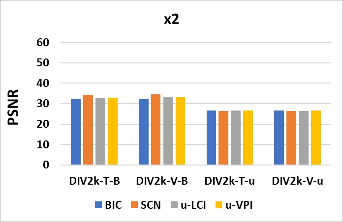
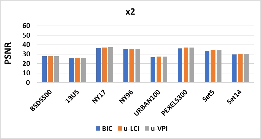
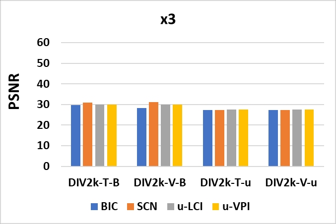
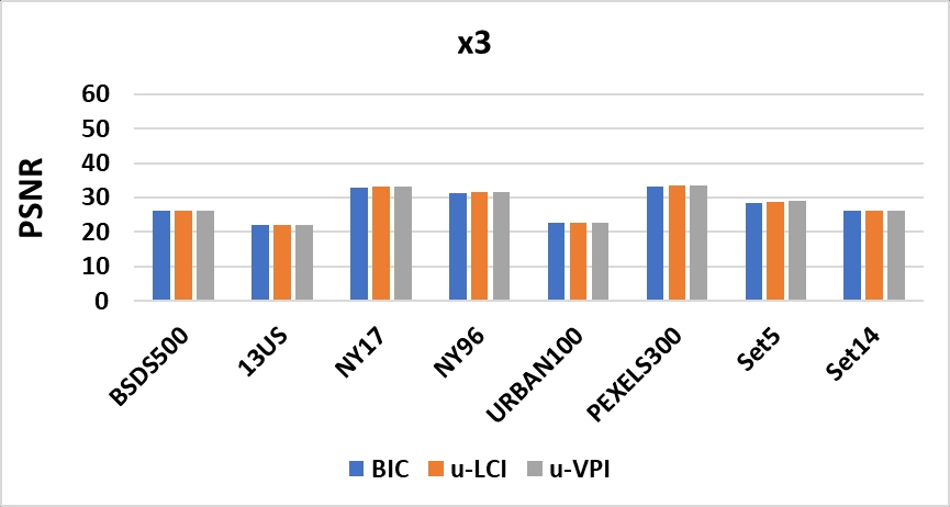
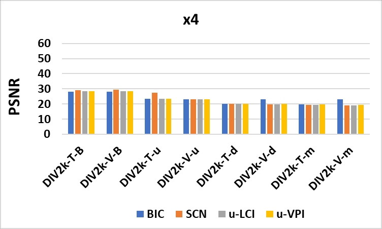
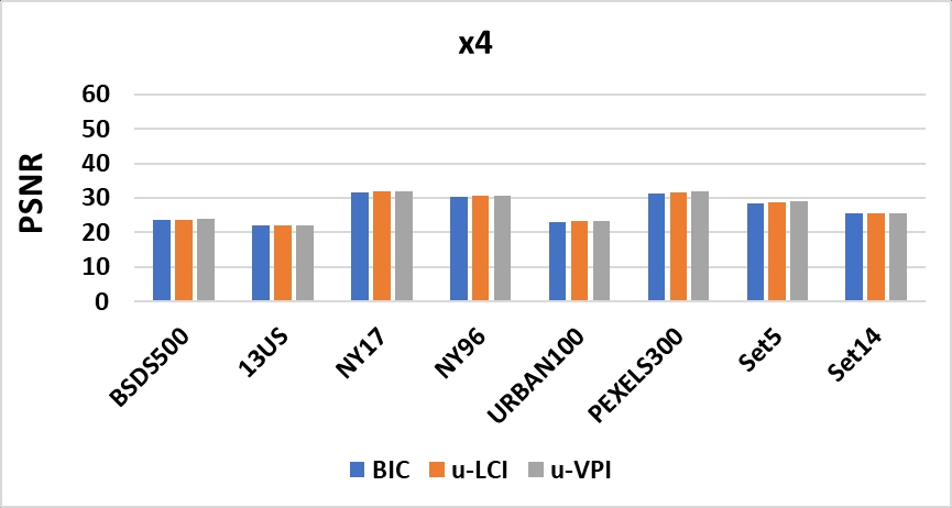
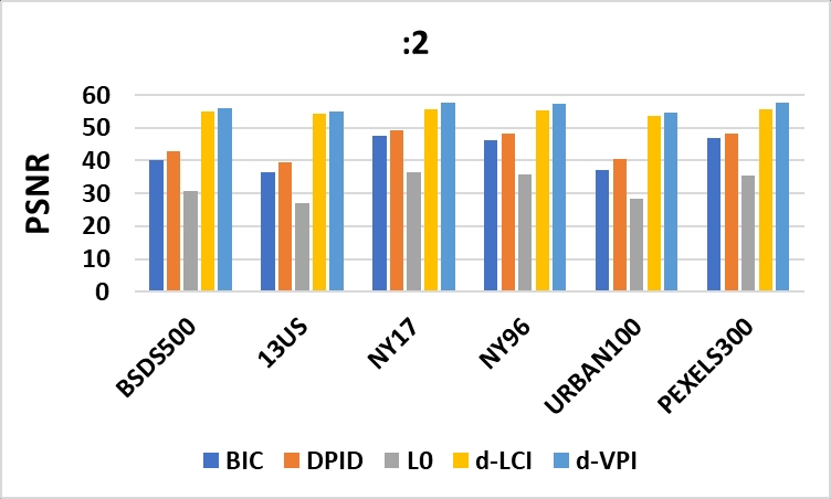
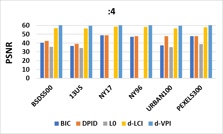
Figure 4: PSNR values extracted from Tables 1–4

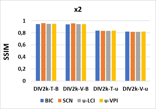
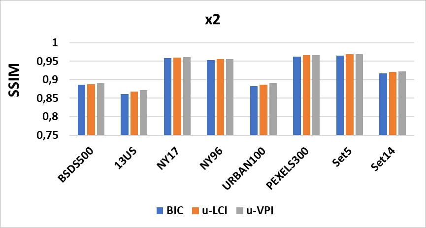
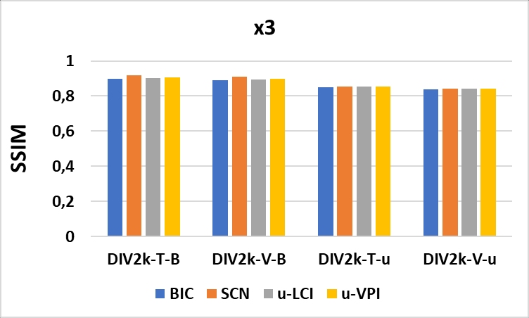
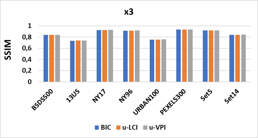
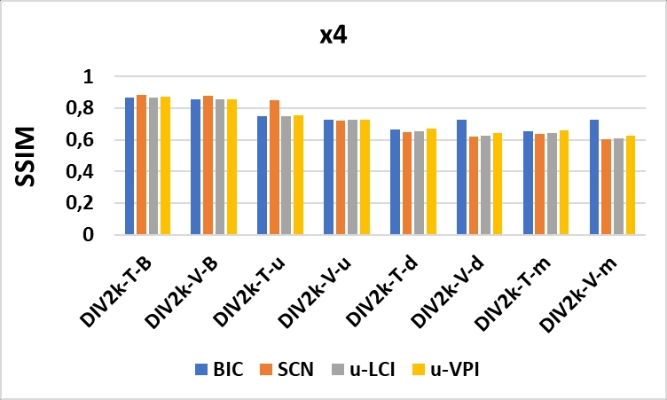
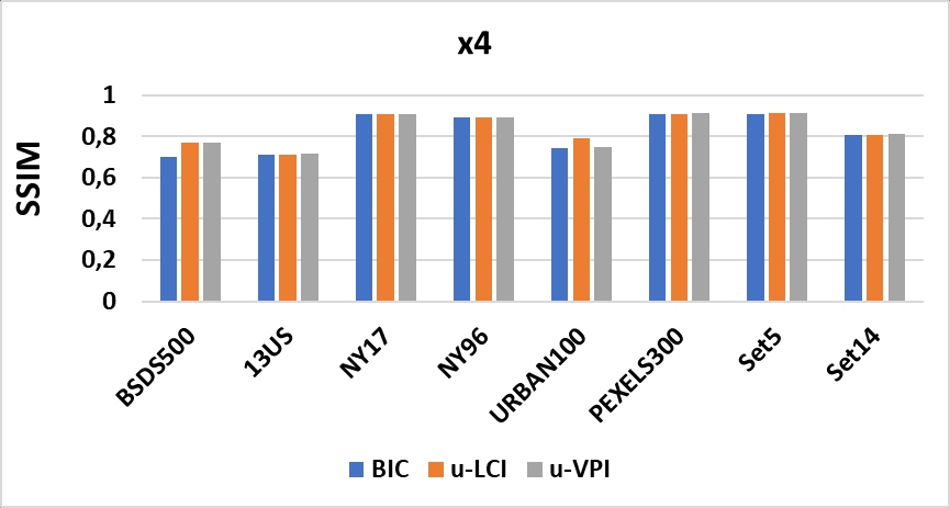
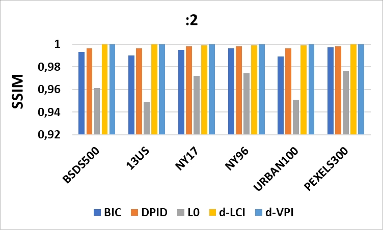
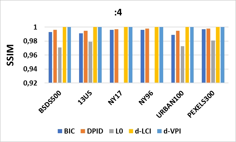
Figure 5: SSIM values extracted from Tables 1–4

From the displayed average results, we observe the following.
$\Box$ Concerning upscaling:

1. On the datasets displayed in Table 3, employing the methods with BIC input images, u-VPI has a slightly higher performance than BIC and u-LCI in terms of the visual quality values;

2. On the DIV2k dataset, providing the input images from the datasets therein included, we observe that the previous trend for BIC, u-LCI, and u-VPI is confirmed. However, we also find SCN that gives the best visual quality values when the input images are generated by BIC (i.e., belonging to DIV2k-T-B and DIV2k-V-B datasets). Nevertheless, in the case of input images classified unknown (i.e., belonging to DIV2k-T-u and DIV2k-V-u datasets), slightly higher performance values are given by u-VPI, except in one case. Indeed, SCN has the best performance on DIV2k-T-u when s=4. On the contrary, SCN always provides the lowest PSNR and SSIM values when the input images are classified as both difficult and mild (see Table 2). In this case, u-VPI continues to provide the best quality values for the Train images (i.e., for input images in DIV2k-T-d and DIV2k-T-m). However, BIC outperforms it for the Valid images (i.e., with input images from DIV2k-V-d and DIV2k-V-m). Finally, no change regards the comparison u-VPI / u-LCI, where u-VPI always gives slightly higher values.

Table 5: Average of the optimal values of $\theta$ resulting from supervised-VPI with BIC input images. The downscaling $:3$ case is missing since it is independent of $\theta$

	:2	:4	x2	x3	x4
BSDS500	0,279	0,649	0,198	0,203	0,543
13US	0,250	0,250	0,135	0,288	0,142
NY17	0,374	0,688	0,132	0,150	0,153
NY96	0,363	0,678	0,146	0,193	0,183
Urban100	0,251	0,596	0,127	0,264	0,135
Pexels300	0,370	0,596	0,118	0,122	0,121
Set 5			0,110	0,250	0,120
Set 14			0,121	0,108	0,188
DIV2k-T-B			0,113	0,125	0,125
DIV2k-V-B			0,114	0,123	0,121
DIV2k-T-u			0,607	0,098	0,717
DIV2k-V-u			0,609	0,093	0,722
DIV2k-T-d					0,894
DIV2k-V-d					0,896
DIV2k-T-m					0,892
DIV2k-V-m					0,912

Figure 6: Boxplot derived from Table 5

$\Box$ Concerning downscaling (with BIC input images):

1. The best PSNR and SSIM values are achieved by d-VPI, followed in order by d-LCI (ex-aequo in some cases), DPID, BIC, and L₀. For all datasets and scale factors displayed in Table 3, there is a consistent gap between the PSNR values by d-VPI and those provided by BIC, DPID, and $L_{0}$. According to the results in Lagrange , also d-LCI provides good values, but generally, d-VPI outperforms it, even if with a smaller gap.

2. The demo version of $L_{0}$ has memory problems with input images of large size. In fact, in the case of target images from $NY17$ and $NY96$ datasets, $L_{0}$ does not give any output for the scale factor $s=2,3$ that, according to (38), generate a large input size.

3. When $s=3$, d-VPI confirms the optimal performance proved in Proposition 1 for odd scaling factors. We note that this case is missing in Figures 4–5 since (29) holds for both d-LCI and d-VPI. Nevertheless, we point out that (29) has been proved under the ideal assumptions that the required LR sampling satisfies the Nyquist–Shannon theorem and that the initial data are not corrupted. Hence it is not always true. Indeed, we have verified (29) continues to hold starting from HR input images generated by the Nearest-Neighbor and Bilinear methods NN-NIL2 (using Matlab imresize with nearest and bilinear option respectively), but in Subsection 5.2.3 we show it does not hold if we use SCN to generate the input HR image.

5.2.1 Parameter modulation

In this subsection, we use the previous quantitative analysis to hint to the user for setting the parameter $\theta$ in practice when the target image is unavailable.

To this aim, in the previous tests employing supervised VPI with BIC input images, for each dataset, we compute the average of the optimal values of $\theta$ corresponding to the output images presenting the minimal MSE. For both upscaling and downscaling, we report these results in Table 5 and show the relative boxplot in Figure 6. We remark that the downscaling case with scale factor $s=3$ is missing since, as previously stated, the d-VPI output is independent of $\theta$.

Table 6: Average CPU time in the upscaling cases of Table 3

	x2	x3	x4
BSDS500
BIC	0,003	0,002	0,003
u-LCI	0,014	0,010	0,008
u-VPI	0,013	0,012	0,010
13US
BIC	0,002	0,002	0,002
u-LCI	0,012	0,010	0,009
u-VPI	0,014	0,009	0,012
NY17
BIC	0,091	0,074	0,071
u-LCI	1,357	0,839	0,634
u-VPI	1,314	0,930	0,732
NY96
BIC	0,056	0,055	0,051
u-LCI	0,812	0,567	0,459
u-VPI	0,864	0,606	0,487
URBAN100
BIC	0,009	0,008	0,008
u-LCI	0,051	0,051	0,059
u-VPI	0,076	0,058	0,050
PEXELS300
BIC	0,041	0,037	0,035
u-LCI	0,300	0,216	0,185
u-VPI	0,366	0,300	0,255
SET5
BIC	0,003	0,003	0,002
u-LCI	0,014	0,008	0,006
u-VPI	0,015	0,009	0,009
SET14
BIC	0,003	0,003	0,005
u-LCI	0,020	0,014	0,013
u-VPI	0,022	0,017	0,015

Table 7: Average CPU time in the upscaling cases of Tables 1–2

	x2	x3	x4
DIV2k-T-B
BIC	0,036	0,031	0,032
SCN	14,353	30,972	17,879
u-LCI	0,245	0,175	0,165
u-VPI	0,318	0,225	0,187
DIV2k-V-B
BIC	0,035	0,029	0,030
SCN	14,822	32,872	18,855
u-LCI	0,252	0,197	0,152
u-VPI	0,315	0,234	0,192
DIV2k-T-u
BIC	0,035	0,025	0,023
SCN	14,442	29,500	17,568
u-LCI	0,233	0,176	0,149
u-VPI	0,322	0,224	0,190
DIV2k-V-u
BIC	0,029	0,029	0,027
SCN	14,976	32,270	18,362
u-LCI	0,248	0,179	0,147
u-VPI	0,333	0,231	0,214
DIV2k-T-d
BIC			0,022
SCN			17,842
u-LCI			0,150
u-VPI			0,206
DIV2k-V-d
BIC			0,023
SCN			17,608
u-LCI			0,151
u-VPI			0,211
DIV2k-T-m
BIC			0,024
SCN			18,532
u-LCI			0,150
u-VPI			0,206
DIV2k-V-m
BIC			0,024
SCN			18,496
u-LCI			0,150
u-VPI			0,213

Table 8: Average CPU time in downscaling tests of Table 4 (oom denotes ”out of memory”).

	:2	:3	:4
BSDS500
BIC	0,006	0,009	0,017
DPID	7,696	12,246	18,615
L0	3,647	8,020	14,295
d-LCI	0,057	0,001	0,137
d-VPI	0,046	0,001	0,117
13US
BIC	0,005	0,009	0,013
DPID	5,593	8,905	13,819
L0	2,572	5,706	9,939
d-LCI	0,042	0,001	0,108
d-VPI	0,034	0,001	0,086
NY17
BIC	0,229	0,325	0,639
DPID	448,023	731,498	1.098,113
L0	208,574	617,386	oom
d-LCI	6,614	0,023	22,859
d-VPI	7,246	0,023	20,194
NY96
BIC	0,155	0,219	0,422
DPID	291,68	479,638	714,908
L0	133,19	oom	om
d-LCI	4,698	0,016	13,898
d-VPI	4,704	0,016	13,949
URBAN100
BIC	0,027	0,041	0,068
DPID	37,592	60,834	93,996
L0	13,267	28,845	50,312
d-LCI	0,234	0,002	0,618
d-VPI	0,259	0,002	0,732
PEXELS300
BIC	0,088	0,120	0,225
DPID	151,800	246,573	374,155
L0	56,454	125,413	228,683
d-LCI	1,560	0,009	4,977
d-VPI	1,689	0,009	4,406

5.2.2 CPU time analysis

The CPU time required by each scaling method is also an important aspect to consider in the quantitative performance evaluation. For this reason, in the previous experiments, besides PSNR and SSIM, we measure the CPU time each method takes to produce the output images. Tables 6–8 show the average CPU time values we computed, for each scaling factor and dataset, by employing the displayed methods, in upscaling (Tables 6, 7) and downscaling (Table 8).

Regarding VPI, we point out that in Tables 1–4 we tested supervised VPI that is optimally structured to produce 19 resized images corresponding to unsupervised VPI called with 19 equidistant values of the input parameter $\theta$. For this reason, in comparison with the benchmark methods, we report in Tables 6–8 the average CPU time that unsupervised VPI takes, providing in input the average values of $\theta$ reported in Table 5 for each employed datasets and scale factors 2,3,4. For other values of $\theta$, we did not observe significant variations w.r.t. the displayed results.

Inspecting Tables 6–8, we observe the following.
$\Box$ Concerning upscaling:
The method requiring the least CPU time is BIC. At a short distance, we find u-LCI and u-VPI with CPU times very close to each other. Much higher computation time is required by SCN, which always requires the longest CPU time. Table 7 shows that this trend is independent of how the input image is generated (i.e., -B, -u, -d, -m).
$\Box$ Concerning downscaling:
Even in this case, the method requiring the least computation time is BIC, closely followed by d-LCI and d-VPI that coincide and are much faster when the scale factor is 3, due to (33). In the ranking, $L_{0}$ and DPID follow with much higher computation time than d-VPI, especially on datasets characterized by larger image sizes (such as NY17, NY96, and PEXELS300). In particular, $L_{0}$ does not give any output for target images in NY96 and NY17 with scale factors $s\geq 2$ and $s\geq 3$, respectively, while it is faster than DPID in the remaining cases.

Table 9: Average performance results of upscaling methods (first column) on PEXELS300 dataset with input images generated by BIC, u-LCI, u-VPI, DPID and $L_{0}$

	BIC input image		LCI input image		VPI input image		DPID input image		$L_{0}$ input image
	PSNR	SSIM	PSNR	SSIM	PSNR	SSIM	PSNR	SSIM	PSNR	SSIM
x2
BIC	36.249	0.962	36.274	0.963	37.047	0.968	36.336	0.966	35.194	0.964
u-LCI	37.067	0.966	35.302	0.950	36.436	0.959	35.567	0.957	33.589	0.945
u-VPI	37.128	0.966	36.482	0.964	37.397	0.969	36.427	0.966	35.230	0.964
SCN	37.916	0.971	33.939	0.945	35.184	0.957	34.325	0.953	31.818	0.936
x3
BIC	33.147	0.932	32.409	0.929	32.409	0.929	32.988	0.935	32.055	0.929
u-LCI	33.622	0.935	31.444	0.908	31.444	0.908	32.494	0.924	31.173	0.913
u-VPI	33.671	0.936	32.535	0.930	32.535	0.930	33.050	0.935	32.048	0.928
SCN	34.462	0.944	30.245	0.904	30.245	0.904	31.849	0.926	30.145	0.906
x4
BIC	31.374	0.908	30.333	0.903	30.589	0.907	31.113	0.910	31.406	0.913
u-LCI	31.741	0.910	29.414	0.880	29.721	0.885	30.689	0.899	31.001	0.901
u-VPI	31.786	0.912	30.458	0.905	30.683	0.908	31.151	0.910	31.473	0.913
SCN	32.551	0.922	28.147	0.872	28.585	0.882	30.098	0.902	30.619	0.907

Table 10: Average performance results of downscaling methods (first column) on BSDS500 dataset with input images generated by BIC, d-LCI, d-VPI and SCN

	BIC input image		LCI input image		VPI input image		SCN input image
	PSNR	SSIM	PSNR	SSIM	PSNR	SSIM	PSNR	SSIM
:2
BIC	40.080	0.992	42.906	0.996	40.610	0.993	47.910	0.999
d-LCI	54.840	1.000	57.392	1.000	58.509	1.000	36.931	0.987
d-VPI	55.993	1.000	62.467	1.000	61.901	1.000	46.983	0.999
DPID	41.065	0.991	40.256	0.990	40.942	0.991	37.173	0.985
$L_{0}$	37.539	0.990	36.943	0.989	37.250	0.989	32.057	0.966
:3
BIC	40.452	0.993	43.325	0.996	40.860	0.994	47.453	0.999
d-LCI	$\mathbf{\infty}$	1.000	$\mathbf{\infty}$	1.000	$\mathbf{\infty}$	1.000	36.643	0.986
d-VPI	$\mathbf{\infty}$	1.000	$\mathbf{\infty}$	1.000	$\mathbf{\infty}$	1.000	36.643	0.986
DPID	42.282	0.994	40.981	0.992	42.021	0.994	38.212	0.988
$L_{0}$	36.828	0.987	36.348	0.985	36.680	0.986	33.027	0.969
:4
BIC	40.383	0.993	43.218	0.996	40.806	0.994	47.501	0.999
d-LCI	56.846	1.000	59.981	1.000	60.319	1.000	35.911	0.984
d-VPI	60.861	1.000	$\mathbf{\infty}$	1.000	71.533	1.000	40.619	0.994
DPID	42.281	0.994	40.735	0.993	41.991	0.994	38.165	0.989
$L_{0}$	45.123	0.997	46.087	0.998	45.449	0.998	38.712	0.991

5.2.3 Input image dependency

In this subsection, we study the dependency of the VPI performance on the way the input images are generated. To this aim, we repeat the previous quantitative analysis computing the average PSNR and SSIM values for supervised VPI and the benchmark methods, but we let vary the scaling method generating the input images from the target ones in the dataset. More precisely, in downscaling we provide input HR images generated from BIC, u-LCI, u-VPI, and SCN upscaling methods, while in upscaling we get the input LR image by applying the downscaling methods BIC, d-LCI, d-VPI, DPID, and $L_{0}$. We point out that whenever u-VPI or d-VPI are employed to generate the input image, we use the unsupervised mode with the default value $\theta=0.5$.

As above, we consider the scale factors $s=2,3,4$ and we require for the input images the size $n_{1}\times n_{2}$, determined by (38), where $N_{1}\times N_{2}$ is the size of the target images in the dataset.

Since we have experimented that demo codes of $L_{0}$ and SCN have problems in processing images with a large size, we do not consider all datasets for this test, but we focus on PEXELS300 dataset in upscaling and on BSDS500 dataset in downscaling. The average performance results are shown in Tables 9 and 10, respectively.

From these tables, we observe the following.
$\Box$ Concerning upscaling:

• SCN provides the highest quality measures only in the case of BIC input images, confirming the trend displayed in Table 1.

• In the case of input images generated by downscaling methods different from BIC, SCN always provides the lowest values and the best performance is attained by u-VPI except in the upscaling x4 case with $L_{0}$ input images when BIC presents slightly higher performance values than u-VPI.

• Similarly to BIC, u-VPI has a more stable behavior with respect to variations of the input image. The quality measures by u-VPI are always higher than those by u-LCI that behave better than BIC only with BIC input images.

• In upscaling (x3), we note the same performance values for u-LCI and u-VPI input images (3th and 4th columns of Table 9), confirming that in downscaling (:3), both d-LCI and d-VPI generate the same input images.

$\Box$ Concerning downscaling:

• For even scale factors ($s=2,4$), d-VPI always provides much higher performance values than DPID and $L_{0},$ which always presents the lowest quality measures. The d-VPI method followed by d-LCI achieves the highest performance, unless in the case of SCN input images where BIC holds the record, followed in order by d-VPI, DPID, d-LCI, and $L_{0}$ For odd scale factors, it is confirmed that d-VPI reduces to d-LCI reaching the optimal quality measures in the case of input images generated by BIC, u-LCI, or u-VPI. Nevertheless, for SCN input images, the ranking of the even cases $s=2,4$ is confirmed, i.e., the best performance is given by BIC, followed in order by DPID, d-LCI = d-VPI, and $L_{0}.$

5.3 Qualitative evaluation

We test VPI and the benchmark methods for scale factors varying from 2 to very large values both for supervised and unsupervised mode. In this subsection, some visual results of the numerous performed tests are given.
$\bullet$ Concerning the supervised mode:
we show some examples of performance results in Figures 7-8 for upscaling and in Figures 9-10 for downscaling with different BIC input images and scale factors 2, 3, 4. In these figures, some Regions of Interest (ROI) are shown in order to highlight the results at a perceptual level. The visual inspection of these performance results confirms the quantitative evaluation in terms of PSSNR and SSIM exhibited in Subsection 5.2. Hence, we deduce that: a) the observable structure of the objects is captured; b) local contrast and luminance of the input image are preserved; c) small details and most of the salient edges are maintained; d) the presence of ringing and over smoothing artifacts is very limited; e) the resized image is sufficiently not blurred.
$\bullet$ Concerning the unsupervised mode:
we set, as default, the free parameter $\theta$ equal to 0.5 and take the input images directly from the datasets. Unlike the supervised mode, we cannot compute the PSNR and SSIM quality measures since the target image is missing. Consequently, in the following, we evaluate the performance according to our absolute human perceptual ability taking into account the CPU time (briefly denoted by T) when the results are almost equivalent in terms of perceived quality.

Firstly, we consider as input two images already displayed for the supervised mode and used in that case as target images (see Figure 7 and Figure 9). We show the performance results at the scale factor 2 (upscaling) in Figure 11 and at the scale factor 4 (downscaling) in Figure 12. A careful examination of Figure 11 does not highlight significant perceptual visual differences in the upscaled images produced by all methods. However, the required CPU times for u-VPI, u-LCI, and BIC are very close, while SCN takes much more processing time. On the other hand, since the input image in Figure 12 has too high-frequency details, differently from Figure 9 achieved by BIC input image, aliasing effects are visually detectable for all methods. In particular, d-LCI and d-VPI present more evident aliasing effects than the other methods, although with a minor CPU time with respect to L₀ and DPID.

Even if avoiding aliasing effects is an important part of downscaling methods, this is out of the aim of the present paper, which intends to show a different point of view for both upscaling and downscaling by using a specific Approximation Theory tool in the Image Processing framework. Consequently, in Figure 12, as well as in the remaining experiments, we just show the performance result obtained by a pre-filtering combined with d-VPI (denoted as f-d-VPI). We point out that in f-d-VPI, the type of filter to employ is selected based on the feature images. Our selection includes the following 2-D filters: a) averaging filter (’average’); b) circular averaging filter (’disk’); c) Gaussian filter (’gaussian’); d) motion (’motion’), they all implemented in Matlab using hspecial to specify the filter type.

As mentioned in Section 4, this solution only partially reduces the aliasing effect in Figure 12. It does not affect the processing time too much since the CPU time of f-d-VPI is much smaller than that of L₀ and DPID, and very close to the CPU time of BIC.

Intending to highlight the aliasing influence, in the sequel, we consider different kinds of input images extracted from PEXELS300 dataset (so having the same input size 1800$\times$1800), and we apply to them unsupervised d-VPI and the benchmark methods with the same downscaling factor.

In Figure 13 downscaling with scaling factor 3 is applied to the images (1640882 and 163064 from PEXELS300) displayed at the top. Some ROIs of the resulting output images are shown in the middle and bottom in order to emphasize the aliasing phenomenon. By visually inspecting of these ROIs, we can check a different behavior of d-VPI that, in this case, coincides with d-LCI being the LR image computed by (37). Indeed, we note that for the input image on the right (163064) the aliasing effect is not appreciable (see, for instance, the diagonal line in the ROIs) while it becomes visible for the input image on the left (1640882). In the latter case, we observe aliasing occurs for all methods to a different extent, but BIC, L₀, and DPID have better performance since the downscaled images are affected by aliasing to a lesser extent than d-VPI (see the vertical elements of the railing). However, in the resized image by f-d-VPI, the aliasing effect is equally present with respect to the other methods without a significant computational burden. It results to be the second-fastest method and is competitive with BIC (L₀ and DPID have a greater CPU time).

Finally, in Figure 14, we test all downscaling methods at the scale factor 8 on the input image displayed on the top (3472764 from PEXELS300). In this case, d-VPI and d-LCI produce better visual performance results since the stars in the sky are more adequately preserved in terms of numbers and shape. BIC and L₀ reduce too much the number of stars and introduce a blurring effect, while DPID provides a downscaled image where the stars are almost all reshaped and doubled. Moreover, f-d-VPI seems not to give new insights. Note that the aliasing is visible in other areas of the image (see, for example, the mountain ridge area) with almost the same intensity for all methods. About CPU time, also in this case, DPID and L₀ are the most expensive.

In conclusion, we point out that the aliasing effect does not always occur at the same scale factor and does not always influence the downscaling performance similarly. Moreover, in some contexts, even the downscaling methods designed to reduce the aliasing can result inadequate to manage this problem and can introduce distortions even greater than aliasing itself. In these cases, as well as when the aliasing is not visible and when the quality of the downscaled image is visually equivalent, d-VPI may prove to be preferable since it provides a good compromise in terms of quality and CPU time.

x2                                             x3                                           x4

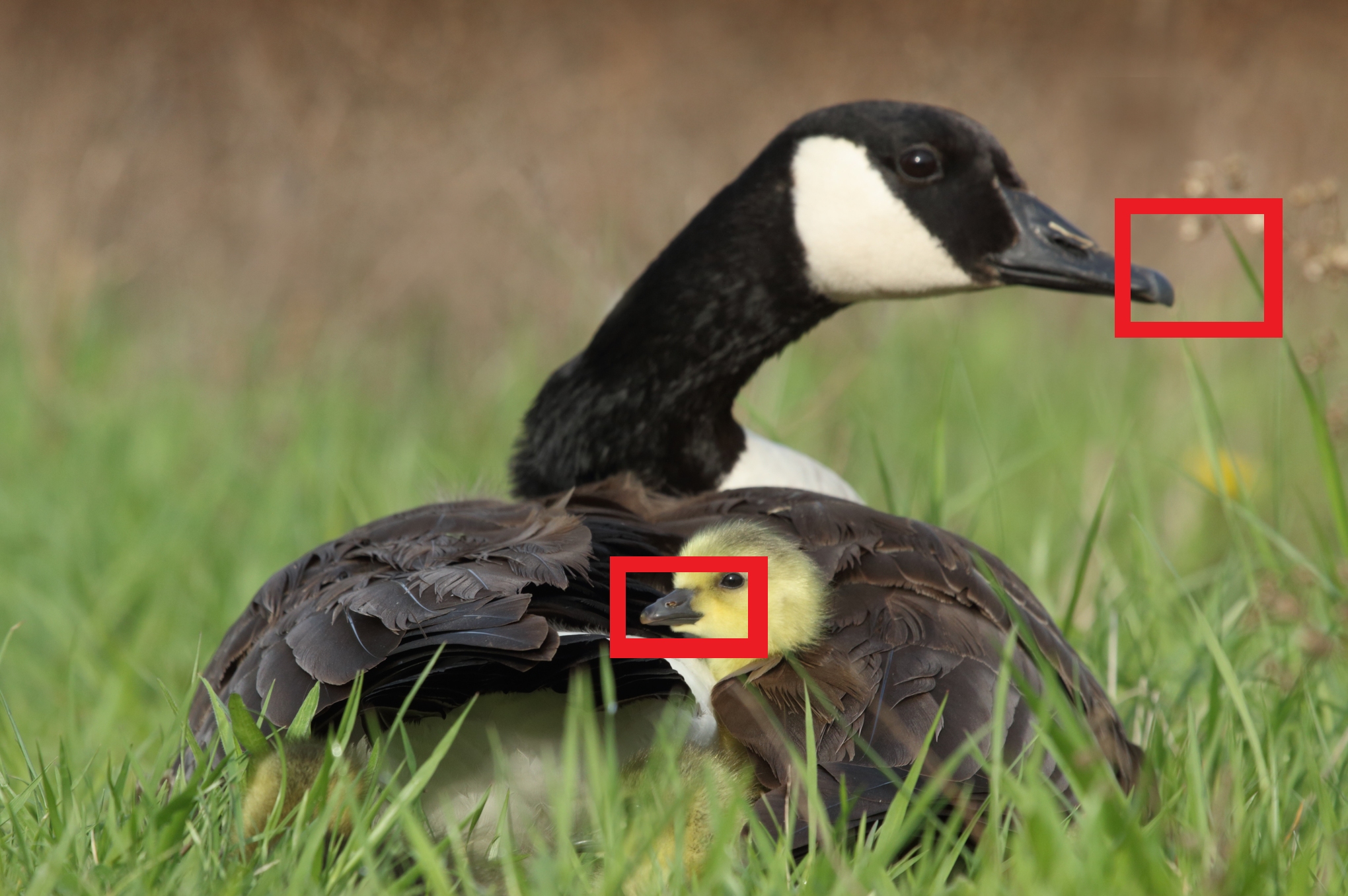
Target image
0023 (1356$\times$2040)	S14.6 (576$\times$720)	N2 (2304$\times$3072)
from DIV2k	from Set14	from NY17

BIC
PSNR=45,773	PSNR=26,204	PSNR=39,220
SSIM=0,995	SSIM=0,811	SSIM=0,952

SCN
PSNR=36,143	PSNR=26,274	PSNR=31,637
SSIM=0,975	SSIM=0,821	SSIM=0,958

Figure 7: Examples of supervised upscaling performance results at the scale factor 2 (left), at the scale factor 3 (middle), at the scale factor 4 (right).

x2                                             x3                                           x4

LCI
PSNR=46,688	PSNR=26,585	PSNR=40,068
SSIM=0,996	SSIM=0,822	SSIM=0,957

VPI
PSNR=46,745	PSNR=26,590	PSNR=40,113
SSIM=0,996	SSIM=0,822	SSIM=0,957

Figure 8: Examples of supervised upscaling performance results at the scale factor 2 (left), at the scale factor 3 (middle), at the scale factor 4 (right).

:2                                             :3                                           :4

Target image
135069 (321$\times$481)	NA38 (480$\times$640)	img075 (680$\times$1024)
from BSDS500	from NY96	from Urban100

BIC
PSNR=50,266	PSNR=39,885	PSNR=41,035
SSIM=1,000	SSIM=0,995	SSIM=0,997

DPID
PSNR=54,342	PSNR=42,037	PSNR=44,545
SSIM=1,000	SSIM=0,997	SSIM=0,999

Figure 9: Examples of supervised downscaling performance results at the scale factor 2 (left), at the scale factor 3 (middle), at the scale factor 4 (right).

:2                                             :3                                           :4

L0
PSNR=39,771	PSNR=33,064	PSNR=37,198
SSIM=0,997	SSIM=0,971	SSIM=0,991

LCI
PSNR=56,984	PSNR=$\infty$	PSNR=57,600
SSIM=1,000	SSIM=1,000	SSIM=1,000

VPI
PSNR=62.452	PSNR=$\infty$	PSNR=62,536
SSIM=1,000	SSIM=1,000	SSIM=1,000

Figure 10: Examples of supervised downscaling performance results at the scale factor 2 (left), at the scale factor 3 (middle), at the scale factor 4 (right). For layout reasons, the performance results both for d-LCI and d-VPI are reported although they coincide for the downscaling factor 3.

BIC (T=0.124)

SCN (T=42,497)

u-LCI (T=1.462)

u-VPI (T=1,698)

Figure 11: An example of unsupervised upscaling performance results at the scale factor 2 on an image extracted from DIV2k (size=1356$\times$2040).

BIC (T=0,018)

DPID (T=5,476)

L0 (T=2,008)

d-LCI (T=0,032)

d-VPI (T=0,033)

f-d-VPI (T=0,133)

Figure 12: An example of unsupervised downscaling performance results at the scale factor 4 on a image extracted from Urban100 (size=680$\times$1024). In f-d-VPI a circular averaging filter with size 3 is employed.

Input images

1640882	163064

BIC	DPID	L0	d-VPI $\equiv$ d-LCI	f-d-VPI

(T=0,029)

(T=30,251)

(T=12,368)

(T=0,002)

(T=0,037)

(T=0,090)

(T=30,116)

(T=13,126)

(T=0,004)

(T=0,125)

Figure 13: Two input images extracted from PEXELS300 (top) and ROIs of unsupervised downscaling performance results at the scale factor 3 (size: 1800$\times$1800) (middle and bottom). In f-d-VPI an average filter is employed.

Input image

3472764

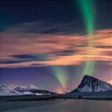
BIC (T=0,031)

DPID (T=22.100)

L0 (T=12,996)

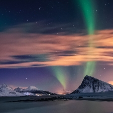
d-LCI (T=0,091)

d-VPI (T=0,113)

f-d-VPI (T=0,137)

Figure 14: Examples of unsupervised downscaling performance results at the scale factor 8 on an input image extracted from PEXELS300 (size 1800$\times$1800). The input image is shown with the same printing size of the resulting images to facilitate the visual comparison. In f-d-VPI an average filter is employed.

6 Conclusions

This paper proposes a new image scaling method, VPI, which is based on non-uniform sampling grids and employs the filtered de la Vallée Poussin type polynomial interpolation at Chebyshev zeros of 1st kind.

The VPI method is simple to implement and highly flexible since it can be applied to resize arbitrary digital images both in upscaling and downscaling by specifying the scale factor or the desired size.

VPI depends on an additional input parameter $\theta\in[0,1]$ that, if necessary, can be suitably modulated to improve the approximation. In particular, taking $\theta=0$, VPI reduces to the LCI method that has been introduced by the authors in Lagrange and is based on classical Lagrange interpolation at the same nodes. Nevertheless, for any $\theta\in]0,1]$ VPI improves the LCI performance and proves to be more stable than the latter due to the uniform boundedness of Lebesgue constants corresponding to the de la Vallée Poussin type interpolation.

The VPI performance has been evaluated using two commonly adopted quality measures, PSNR and SSIM, and measuring the required CPU time too. Comparisons with other recent resizing methods (also specialized in only upscaling or downscaling) have been carried on a wide number of images belonging to several, commonly available, datasets and characterized by different contents and sizes ranging from small to large scale. During the VPI validation procedure, also the modulation of the free parameter $\theta$ has been observed experimentally. Further, the dependency on the input image has been considered by applying to the target images in the datasets different scaling methods in order to generate the input images.

The experimental results confirm that VPI has a competitive and satisfactory performance, with quality measures generally higher and more stable than those of the benchmark methods. Moreover, VPI results much faster than the methods specialized in only downscaling or upscaling, with CPU time close to the one required by LCI and imresize, the Matlab optimized version of bicubic interpolation method (BIC).

At a visual level, VPI captures the object’s visual structure by preserving the salient details, the local contrast, and the luminance of the input image, with well–balanced colors and limited presence of artifacts.

One limitation of VPI concerns downscaling performance when HR images have high–frequency details. Indeed, in downscaling with odd scale factors, VPI produces the same LR image of LCI for any value of $\theta$. In this case, if the Nyquist limit is satisfied, we give a theoretical estimate for the MSE, which, in particular, is null if the input image (or some crucial pixels of it) are ”not corrupted”. Nevertheless, even starting from ”exact” HR images, in downscaling VPI can suffer from aliasing problems when the frequency content of the image and the required size for the LR image are such to violate the Nyquist–Shannon theorem. In our experiments, we report cases when aliasing does not occur and cases when aliasing occurs. In the latter case, we just apply an appropriate filter to the input image before running d-VPI. However, reducing aliasing effects for d-VPI remains an open problem to further investigations.

Funding

The research has been accomplished within RITA (Research ITalian network on Approximation), and UMI (Unione Matematica Italiana) research groups: TAAUMI (Approximation Theory and Applications) and AI&ML&MATUMI (Mathematics for Artificial Intelligence and Machine Learning). It has been partially supported by GNCSINdAM and University of Basilicata (local funds).

Acknowledgements The authors thank the anonymous reviewers for their helpful remarks that allowed to improve the quality of the paper.

Code and supplementary materials

The source code and the dataset PEXELS300 are openly available at the following link:
https://github.com/ImgScaling/VPIscaling.

References

- (1) Arcelli, C., Brancati, N., Frucci, M., Ramella, G., Sanniti di Baja, G.: A fully automatic one-scan adaptive zooming algorithm for color images. Signal Processing 91 (1), 61-71 (2011)
- (2) Atkinson, P.M.: Downscaling in remote sensing. International Journal of Applied Earth Observation and Geoinformation, 22, 106–114 (2013)
- (3) Bevilacqua, M., Roumy, A., Guillemot, C., Alberi-Morel, M. L.: Low-complexity single-image super-resolution based on nonnegative neighbor embedding. In Proc. British Machine Vision Conference (2012)
- (4) Burger, W., Burge, M.J.: Digital Image Processing An Algorithmic Introduction Using Java. Springer (2016)
- (5) Bruni, V.,Ramella, G., Vitulano, D.: An Adaptive Copy-Move Forgery Detection Using Wavelet Coefficients Multiscale Decay. In CAIP 2019, M. Vento, G. Percannella Eds., Lecture Notes in Computer Science 11678, part I, pp. 469-480. Springer (2019)
- (6) Bruni V., Ramella G., Vitulano D. : Automatic Perceptual Color Quantization of Dermoscopic Images. In VISAPP 2015, J. Braz et al. Eds., 1, pp. 323-330. Scitepress Science and Technology Publications (2015)
- (7) Capobianco, M.R., Themistoclakis, W.: Interpolating polynomial wavelets on . Advances in Computational Mathematics, 23(4), 353-374 (2004)
- (8) Chaki J., Dey N.: Introduction to Image Color Feature. In: Image Color Feature Extraction Techniques. SpringerBriefs in Applied Sciences and Technology. Springer, Singapor (2021)
- (9) Chen, H., Lu, M., Ma, Z., Zhang, X., Xu et al.: Learned Resolution Scaling Powered Gaming-as-a-Service at Scale, IEEE Transactions on Multimedia, 23, 584-596 (2021)
- (10) Chen, G., Zhao H., Pang, C. K., Li, T.,Pang, C.: Image Scaling: How Hard Can It Be? IEEEAccess, 7 129452-129465 (2019)
- (11) De Bonis, M.C., Occorsio D., Themistoclakis, W.: Filtered interpolation for solving Prandtl’s integro-differential equations, Numer. Alg. 88 (2), 679–709 (2021)
- (12) De Bonis, M.C., Occorsio, D., Quadrature methods for integro-differential equations of Prandtl’s type in weighted spaces of continuous functions, Appl. Math. and Comput. 393, art. 125721 (2021)
- (13) De Marchi, S., Erb, W., Francomano, E., Marchetti, F., Perracchione, E., Poggiali, D.: Fake Nodes approximation for Magnetic Particle Imaging. In 20th IEEE Mediterranean Electrotechnical Conference, MELECON 2020 - Proceedings, pp. 434-438 (2020)
- (14) Filbir F.,Themistoclakis W.: On the construction of de la Vallée Poussin means for orthogonal polynomials using convolution structures, Journal of Computational Analysis and Applications, 6 (4), 297 - 312 (2004)
- (15) Han, D.: Comparison of Commonly Used Image Interpolation Methods. In Proceedings of the 2nd International Conference on Computer Science and Electronics Engineering, pp. 1556-1559 (2013)
- (16) Hayat, K.: Multimedia super-resolution via deep learning: A survey. Digital SignalProcessing, 81, 198-217 (2018)
- (17) Huang, J.-B., Singh, A., Ahuja, N.: Single image super-resolution from transformed self-examplars. In Proc. CVPR 2015, pp. 5197-5206 (2015)
- (18) Keys, R. G.: Cubic Convolution Interpolation for Digital Image Processing. IEEE Trans. on Acoustics, Speech, and Signal Processing, 29 (6), 1153-1160 (1981)
- (19) Kopf, J., Shamir, A., Peers, P.: Content-adaptive image downscaling. ACM Transactions on Graphics, 32 (6), article 173 (2013)
- (20) Li, X., Wu, Y., Zhang, W., Wang, R., Hou, F.: Deep learning methods in real‑time image super‑resolution: a survey. Journal of Real-Time Image Processing, 17, 1885-1909 (2020)
- (21) Lin, X., Li, J., Wanga, S., Liew, A., Cheng, F., Huang, X.: Recent Advances in Passive Digital Image Security Forensics: A Brief Review, Engineering 4, 29-39 (2018)
- (22) Liu, H., Xie X., Ma, W.Y., Zhang, H.J.: Automatic Browsing of Large Pictures on Mobile Devices. In 11th ACM International Conference on Multimedia, Berkeley, CA, USA, 2003.
- (23) Liu, J., He , S., Lau, R. W. H.: L0Regularized Image Downscaling. IEEE Trans. Image process., 27 (3) (2018)
- (24) Liu, T., Yuan, Z., Sun, J., Wang, J., Zheng, N., Tang, X., Shum, H.-Y.: Learning to detect a salient object, IEEE Trans. on Patt. Anal. Mach. Intell. 33 (2), 353–367 (2011).
- (25) Lookingbill, A., Rogers, J., Lieb, D., Curry, J., Thrun, S.: Reverse Optical Flow for Self-Supervised Adaptive Autonomous Robot Navigation. International Journal of Computer Vision 74 (3), 287–302 (2007)
- (26) Madhukar B.N., Narendra R.: Lanczos Resampling for the Digital Processing of Remotely Sensed Images., in Proc. of International Conference on VLSI, Communication, Advanced Devices, Signals & Systems and Networking (VCASAN-2013). Chakravarthi V., Shirur Y., Prasad R. (eds) . Lecture Notes in Electrical Engineering, vol 258, pp. 403–411. Springer (2013)
- (27) Martin, D., Fowlkes, C., Tal, D., Malik, J.: A database of human segmented natural images and its application to evaluating segmentation algorithms and measuring ecological statistics. In Proc. 8th Int. Conf. Computer Vision, vol.2, pp. 416–423 (2001)
- (28) Mastroianni, G., Russo, M.G., Themistoclakis, W.: The boundedness of the Cauchy singular integral operator in weighted Besov type spaces with uniform norms. Integral Equations Operator Theory 42 (1), 57–89 (2002)
- (29) Mastroianni G., Themistoclakis, W.: De la Vallée Poussin means and Jackson theorem, Acta Sci. Math. (Széged) 74, 147–170 (2008)
- (30) Mastroianni G., Themistoclakis, W.: A numerical method for the generalized airfoil equation based on the de la Vallée Poussin interpolation. J. Comput. Appl. Math. 180, 71–105 (2005)
- (31) Meijering, E.H.W., Niessen, W.J., Viergever, M.A.: Quantitative evaluation of convolution-based methods for medical image interpolation. Medical Image Analysis 5, 111–126 (2001)
- (32) Mittal, H., Pandey, A.C., Saraswat, M. et al. : A comprehensive survey of image segmentation: clustering methods, performance parameters, and benchmark datasets. Multimed Tools Appl, (2021)
- (33) Neetha, C.H., John Moses C., Selvathi D.: Image Interpolation Using Non-adaptive Scaling Algorithms for Multimedia Applications—A Survey, in Advances in Automation, Signal Processing, Instrumentation, and Control, Komanapalli V.L.N., Sivakumaran N., Hampannavar S. (eds), Lecture Notes in Electrical Engineering, vol 700, Springer, pp. 1509-1516 (2021)
- (34) Occorsio, D., Ramella, G., Themistoclakis, W.: Lagrange–-Chebyshev Interpolation for image resizing, Mathematics and Computers in Simulation 197 105 – 126 (2022)
- (35) Occorsio, D., Russo, M.G.: Numerical methods for Fredholm integral equations on the square. Appl. Math. and Comput. 218 (5), 2318–2333 (2011)
- (36) Occorsio, D., Themistoclakis, W.: Some remarks on filtered polynomial interpolation at chebyshev nodes, Dolomites Research Notes on Approximation, 14, 68–84 (2021)
- (37) Occorsio, D., Themistoclakis, W.: On the filtered polynomial interpolation at Chebyshev nodes, Applied Numerical Mathematics, 166, 272 – 287 (2021)
- (38) Occorsio, D., Themistoclakis, W.: Uniform weighted approximation on the square by polynomial interpolation at Chebyshev nodes. Applied Mathematics and Computation, 385, doi=10.1016/j.amc.2020.125457, art. n. 125457 (2020)
- (39) Occorsio, D., Themistoclaki,s W.: Uniform Weighted Approximation by Multivariate Filtered Polynomials, Lecture Notes in Computer Science, 11973, pp. 86 –100 (2020)
- (40) Occorsio, D., Russo, M.G., Themistoclakis, W.: Filtered integration rules for finite Hilbert transform, arxiv:2109.10634 (2021)
- (41) Occorsio, D., Russo, M.G., Themistoclakis, W.: Filtered integration rules for finite weighted Hilbert transform, submitted (2022)
- (42) Oztireli, A. C., Gross, M.: Perceptually based downscaling of images, ACM Trans. Graph. 34 (4), Article 77, (2015)
- (43) Poggiali, D., Cecchin, D., Campi, C., De Marchi, S.: Oversampling errors in multimodal medical imaging are due to the Gibbs effect, Mathematics 9 (12), art. number 1348 (2021)
- (44) Pratt, W.K.: Digital Image Processing. John Wiley & Sons, New York (2001)
- (45) Ramella G., Sanniti di Baja G.: Color histogram-based image segmentation. In Computer Analysis of Images and Patterns – CAIP 2011, P. Real, D. Diaz-Pernil, H. Molina-Abril, A. Berciano, W. Kropatsch Eds., Lecture Notes in Computer Science 6854, Springer, I, pp. 76–83 (2011)
- (46) Ramella, G., Sanniti di Baja, G.: Image segmentation based on representative colors and region merging. In Pattern Recognition, J. A. Carrasco-Ochoa et al Eds., 611 Lecture Notes in Computer Science 7914, Springer, pp. 175–184 (2013)
- (47) Ramella, G., Sanniti di Baja, G.: From color quantization to image segmentation. In Proc. 12th Internat. Conf. Signal Imag. Techn. Internet-Based Syst. - SITIS 2016, K. Yetongnon et al. Eds., IEEE Computer Society, pp. 798-804 (2016)
- (48) Ramella, G.: Evaluation of quality measures for color quantization, Multimedia Tools and Applications,80 (21-23), 32975 –33009 (2021)
- (49) Ramella, G., Sanniti di Baja, G.: A new technique for color quantization based on histogram analysis and clustering. Int. J. Patt. Recog. Artif. Intell. 27 (3), 1–17 (2013)
- (50) Ramella, G., Sanniti di Baja, G.: A new method for color quantization. In Proc. 12th Intern. Conf. Signal Imag. Techn. Internet-Based Syst. - SITIS 2016, K. Yetongnon et al. Eds., IEEE Computer Society, pp. 1–6 (2016)
- (51) Setlur, V., Takagi, S., Raskar, R., Gleicher, M., Gooch, B.: Automatic image retargeting. In Proceedings of the 4th international conference on Mobile and ubiquitous multimedia, pp. 59–68 (2005)
- (52) Stentiford, F. W. M., Attention based auto image cropping. In Proc. 5th International Conference on Computer Vision Systems, Bielefeld (2007)
- (53) Themistoclakis, W.: Uniform approximation on via discrete de la Vallée Poussin means, Numerical Algorithms, 60 (4), 593 –612 (2012)
- (54) Themistoclakis, W.: Weighted approximation on via discrete de la Vallée Poussin mean. Mathematics and Computers in Simulation, 147, 279–292 (2018)
- (55) Themistoclakis, W.: Some error bounds for Gauss-Jacobi quadrature rules. Appl. Numer. Math.116, 286–293 (2017)
- (56) Themistoclakis, W., Van Barel, M.: Generalized de la Vallée Poussin approximations on , Numerical Algorithms, 75 (1), 1–31 (2017)
- (57) Thomee, B., Shamma, D. A., Friedland, G., Elizalde, B., Ni, K., Poland, D., Borth, D., Li, L.-J.: YFCC100M: The new data in multimedia research. Communications of the ACM 59 (2), (2016)
- (58) Timofte, R., Agustsson, E., Van Gool, L., Yang, M.-H.,Zhang, L., et al.: Ntire 2017 challenge on single image super-resolution: Methods and results. In the IEEE Conferenceon Computer Vision and Pattern Recognition (CVPR) Workshop, (2017)
- (59) Unser, M., Aldroubi, A., Eden, M.: Fast B-Spline Transforms for Continuous Image Representation and Interpolation. IEEE Transactions on Pattern Analysis and Machine Intelligence 13 (3), 277–285 (1991)
- (60) Vlas̆ic, T. , Ralas̆ic, I. , Tafro, A., Sers̆ic, D.: Spline-like Chebyshev polynomial model for compressive imaging, J. Vis. Commun. Image R, 66 (2020)
- (61) Wang, Z., Liu, D., Yang, J., Han, W., Huang, T.: Deep networks for image super-resolution with sparse prior. IEEE International Conference on Computer Vision, (2015)
- (62) Wang Z., Bovik A. C., Sheikh H. R., Simoncelli E. P.: Image quality assessment: from error visibility to structural similarity. IEEE Trans. Imag. Proc. 2004, 13 (4), 600–612 (2004)
- (63) Weber, N., Waechter, M., Amend, S. C., Guthe, S.,Goesele, M., Rapid, Detail-Preserving Image Downscaling, ACM Trans. Graph., 35 (6), article number 205 (2016)
- (64) Xiao, Q., Chen, Y., Shen, C.,Chen, Y., Li, K.: Seeing is not believing: Camouflage attacks on image scaling algorithms. In Proc. of the 28th USENIX Security Symposium, pp. 443 - 460 (2019)
- (65) Yang, J., Wright, J., Huang, T. et al.: Image super-resolution via sparse representation. IEEE Trans. Image Process., 19 (11) (2010)
- (66) Yang , W., Zhang , X., Tian, Y., Wang , W., Xue, J.-H., Liao, Q.: Deep Learning for Single Image Super-Resolution: A Brief Review. IEEE Trans. on Multimedia 21 (12) (2019)
- (67) Yao T., Luo Y., Chen Y., Yang D., Zhao L.: Single-Image Super-Resolution: A Survey. In Communications, Signal Processing, and Systems. CSPS 2018. Liang Q., Liu X., Na Z., Wang W., Mu J., Zhang B. (eds) , Lecture Notes in Electrical Engineering, vol 516, Springer, pp. 119–125 (2020)
- (68) Zeyde, R., Elad, M., Protter, M.: On single image scale-up using sparse-representations. In Proc. International Conference on Curves and Surfaces, pp. 711–-730 (2010)
- (69) Zhang, M., Zhang, L., Sun, Y., Feng, L., Ma, W.: Auto cropping for digital photographs. In 2005 IEEE International Conference on Multimedia and Expo, pp. 4 (2005)
- (70) Zhou, D.-X.: Theory of deep convolutional neural networks: Downsampling. Neural Networks 124, 319–327 (2020)
- (71) Plonka, G., Potts, D., Steidl, G., Tasche, M.: Numerical Fourier Analysis. In Applied and Numerical Harmonic Analysis, Birkhüser Springer Nature Switzerland AG, Berlin, (2018)
- (72) Shannon, C.: Communication in the presence of noise. In Proc. of the Institute of Radio Engineers 37, 1, pp. 10–21 (1949)
- (73) Wolberg, G.: Digital Image Warping, IEEE Computer Society Press, Los Alamitos, CA, USA, (1990)
- (74) https://it.mathworks.com/help/vision/ref/psnr.html
- (75) www2.eecs.berkeley.edu/Research/Projects/CS/vision/bsds/
- (76) https://www.cl.cam.ac.uk/ aco41/Files/Sig15UserStudyImages.html
- (77) National Aeronautics and Space Administration, 2016. NASA image gallery. https://www.nasa.gov/multimedia/imagegallery/index.html
- (78) https://www.gcc.tu-darmstadt.de/home/proj/dpid/index.en.jsp
- (79) https://paperswithcode.com/dataset/set5
- (80) https://paperswithcode.com/dataset/set14
- (81) https://data.vision.ee.ethz.ch/cvl/DIV2K/
- (82) https://www.pexels.com/search/color/