Abstract

We present PAC-Bayesian bounds for the generalisation error of the $K$-nearest-neighbour classifier ($K$-NN). This is achieved by casting the $K$-NN classifier into a kernel space framework in the limit of vanishing kernel bandwidth. We establish a relation between prior measures over the coefficients in the kernel expansion and the induced measure on the weight vectors in kernel space. Defining a sparse prior over the coefficients allows the application of a PAC-Bayesian folk theorem that leads to a generalisation bound that is a function of the number of redundant training examples: those that can be left out without changing the solution. The presented bound requires to quantify a prior belief in the sparseness of the solution and is evaluated after learning when the actual redundancy level is known. Even for small sample size ($m\approx 100$) the bound gives non-trivial results when both the expected sparseness and the actual redundancy are high.

1 Introduction

The $K$-nearest-neighbour ($K$-NN) [Fix and HodgesFix and Hodges1951a, Fix and HodgesFix and Hodges1951b] classifier is an elegantly simple and surprisingly effective learning machine. It takes as input a set of training objects and their labels, and returns for a given test object represented in terms of its pairwise distances to the training objects a label that is determined by a majority vote over the labels of the $K$ nearest neighbours in the training sample. $K$-NN is not only conceptually simple but also very versatile because it does not require a vectorial representation but only the pairwise distances between test and training objects. It is thus applicable to all kinds of structural data like strings or graphs as long as a meaningful (in the sense of the classification task) distance measure can be defined. $K$-NN also has some remarkable asymptotic properties. It is universally consistent in the sense that it converges to the Bayes decision if $K\rightarrow\infty$ and $K/m\rightarrow 0$ as the training sample size $m\rightarrow\infty$. Also under certain regularity conditions the risk of $1$-NN for $m\rightarrow\infty$ is bounded from above by twice the Bayes error, $R_{\infty}\left(\mathrm{NN}_{1}\right)\leq 2R\left(h_{\mathrm{Bayes}}\right)$, while for $K$-NN it can be shown that $R_{\infty}\left(\mathrm{NN}_{K}\right)\leq R\left(h_{\mathrm{Bayes}}\right)(1+\sqrt{2/K})$. With regard to the computational effort a simple analysis yields $\mathcal{O}\left(mKd\right)$ where $d$ represents the cost of one distance evaluation. More refined analysis reveals that for fixed $K$ and $d$ the worst case time is $\mathcal{O}\left(m^{1/d}\right)$ and the expected time is $\mathcal{O}\left(\log m\right)$. These results and more regarding $K$-NN can be found in [Devroye, Györfi, and LugosiDevroye et al.1996].

In this paper we will be concerned with bounds on the risk of the $K$-NN classifier for small sample size. Why should such an analysis be of interest? To answer this question consider the infamous no-free-lunch theorem by Wolpert [WolpertWolpert1995]. This theorem essentially states that averaged over a uniform distribution over all learning problems no classifier is better than any other. This theorem may at first glance leave no hope for the successful development of reliable learning algorithms. More careful analysis, however, reveals that only the objective of developing a universally best learning machine is led ad absurdum. What the theorem does tell us is that given a sample and a learning algorithm we should require the learning algorithm to output not only a classifier but also a performance guarantee: we require the learning algorithm to be self-bounding [FreundFreund1998]. This performance guarantee is best given in terms of an a-posteriori bound on the risk of the classifier. Standard PAC/VC theorems provide a-priori results in the sense that the bound value is entirely determined by the level of confidence $1-\delta$, the number $m$ of training examples, the empirical risk $R_{\mathrm{emp}}$, and the complexity of the hypothesis class $\mathcal{H}$ — usually expressed in terms of its VC-dimension $d_{\mathrm{VC}}$. These bounds can thus be evaluated before learning if $R_{\mathrm{emp}}=0$ is enforced, or after learning when $R_{\mathrm{emp}}$ is known. In contrast, an a-posteriori bound may only be evaluated after learning, because it takes into account the match between the hypothesis class $\mathcal{H}$ and the training data $Z$, e.g. in terms of the margin observed on the training sample.

The idea of a-posteriori bounds was developed in statistical learning theory and the first conceptual framework for such bounds was structural risk minimisation [VapnikVapnik1998]. The idea was further developed to include data-dependent structural risk minimisation [Shawe-Taylor, Bartlett, Williamson, and AnthonyShawe-Taylor et al.1996] that is capable of exploiting luckiness w.r.t. the match of input data and learning machine. The latest results are now known as the PAC-Bayesian framework based on work by David McAllester [McAllesterMcAllester1998]. Note that the PAC-Bayesian framework also provided the basis for the discovery of a very tight margin bound for linear classifiers in kernel spaces [Herbrich, Graepel, and CampbellHerbrich et al.1999].

In Section 2 we introduce basic concepts and notation and present the PAC-Bayesian results on which our analysis is based. In Section 3 we briefly review the definition of the $K$-nearest-neighbour classifier. In Section 4 the $1$-NN algorithm is formulated as the limiting case of a linear classifier in a kernel space. This leads to an intuitive explanation of its generalisation ability. The resulting hypothesis space is then used in Section 5 by defining a sparse prior that leads to a PAC-Bayesian bound for $1$-NN. This result will is generalised to $K$-NN in Section 6. Finally, we conclude and point to ideas for future work by relating $K$-NN to Support Vector Machines (SVM) [VapnikVapnik1998].

Throughout the paper we denote probability measures by $\boldsymbol{\mathsf{P}}_{\mathsf{H}}$ and the related expectation by $\boldsymbol{\mathsf{E}}_{\mathsf{H}}$. The subscript refers to the random variable.

2 Learning in the PAC-Bayesian framework

We consider the learning of binary classifiers. We define learning as the process of selecting one hypothesis $h$ from a given hypothesis space $\mathcal{H}$ of hypotheses $h:\mathcal{O}\rightarrow\mathcal{Y}$ that map objects $\boldsymbol{\mathsf{o}}\in\mathcal{O}$ to labels $y\in\mathcal{Y}=\left\{-1,+1\right\}$. The selection is based on a training sample $Z$ comprised of a set $O=\left\{\boldsymbol{\mathsf{o}}_{1},\ldots,\boldsymbol{\mathsf{o}}_{m}\right\}\in\mathcal{O}^{m}$ of objects and their corresponding labels. We will assume the training sample $Z$ to be drawn iid from a probability measure $\boldsymbol{\mathsf{P}}_{\mathsf{Z}}\equiv\boldsymbol{\mathsf{P}}_{\mathsf{OY}}=\boldsymbol{\mathsf{P}}_{\mathsf{Y}|\mathsf{O}}\boldsymbol{\mathsf{P}}_{\mathsf{O}}$. Based on these definitions let us define the risk $R\left(h\right)$ of a hypothesis $h$ by

$$R\left(h\right)=\boldsymbol{\mathsf{P}}_{\mathsf{Z}}\left[h\left(\mathsf{O}\right)\neq\mathsf{Y}\right]\,.$$

A reasonable criterion for learning is to try to find the the hypothesis $h^{*}=\mathrm{argmin}_{h}R\left(h\right)$ that minimises the risk. The difficulty in this learning task lies in the fact that the probability measure $\boldsymbol{\mathsf{P}}_{\mathsf{Z}}$ is unknown. Let us define the empirical risk $R_{\mathrm{emp}}\left(h,Z\right)$ of an hypothesis $h\in\mathcal{H}$ on a training sample $Z$ by

$$R_{\mathrm{emp}}\left(h,Z\right)=\frac{1}{m}\left|\left\{\left(\boldsymbol{\mathsf{o}},y\right)\in Z:h\left(\boldsymbol{\mathsf{o}}\right)\neq y\right\}\right|\,.$$ (1)

The principle of empirical risk minimisation [VapnikVapnik1998] advocates minimising the empirical risk $R_{\mathrm{emp}}\left(h,Z\right)$ instead of the true risk $R\left(h\right)$.

An a-posteriori bound aims at bounding the risk $R\left(h\right)$ of an hypothesis $h$ based on the knowledge of $\mathcal{H}$ as well as $Z$. We now present two theorems by D. McAllester [McAllesterMcAllester1998] that require the definition of a prior measure $\boldsymbol{\mathsf{P}}_{\mathsf{H}}$ on $\mathcal{H}$ and reward the selection of a hypothesis of high prior weight with a low bound on the generalisation error. Note that these theorems do not depend on the correctness of $\boldsymbol{\mathsf{P}}_{\mathsf{H}}$. If the belief expressed in $\boldsymbol{\mathsf{P}}_{\mathsf{H}}$ turns out to be wrong, the bounds just become trivial.

Theorem 1.

For any probability measure $\boldsymbol{\mathsf{P}}_{\mathsf{H}}$ over an hypothesis space $\mathcal{H}$ containing a target hypothesis $h^{*}\in\mathcal{H}$, and any probability measure $\boldsymbol{\mathsf{P}}_{\mathsf{Z}}$ on labelled objects, we have, for any $\delta>0,$ that with probability at least $1-\delta$ over the selection of a sample $Z$ of $m$ examples, the following holds for all hypotheses $h\in\mathcal{H}$ agreeing with $h^{*}$on that sample:

$$R\left(h\right)\leq\frac{\log\frac{1}{\boldsymbol{\mathsf{P}}_{\mathsf{H}}\left(h\right)}+\log\frac{1}{\delta}}{m}\,.$$

To see that this is true note that the probability that a hypothesis $h$ with risk $R\left(h\right)$ is consistent with a sample of $m$ examples is bounded from above by $\left(1-R\left(h\right)\right)^{m}\leq\exp\left(-mR\left(h\right)\right)$. If $R\left(h\right)$ is greater than the above bound the probability that $h$ is consistent with the sample is bounded from above by $\boldsymbol{\mathsf{P}}_{\mathsf{H}}\left(h\right)\delta.$ Applying the union bound the probability that some hypothesis $h$ that violates the bound is consistent with the sample is bounded by $\sum_{h\in\mathcal{H}}\boldsymbol{\mathsf{P}}_{\mathsf{H}}\left(h\right)\delta=\delta$.

Essentially replacing the binomial tail bound used in the above argument by the Chernoff bound for bounded random variables leads to an agnostic version of the above Theorem 1.

Theorem 2.

For any probability measure $\boldsymbol{\mathsf{P}}_{\mathsf{H}}$ over an hypothesis space $\mathcal{H}$, and any probability measure $\boldsymbol{\mathsf{P}}_{\mathsf{Z}}$ on labelled objects, we have, for any $\delta>0,$ that with probability at least $1-\delta$ over the selection of a sample $Z$ of $m$ examples, all hypotheses $h\in\mathcal{H}$ satisfy

$$R\left(h\right)\leq R_{\mathrm{emp}}\left(h,Z\right)+\sqrt{\frac{\log\frac{1}{\boldsymbol{\mathsf{P}}_{\mathsf{H}}\left(h\right)}+\log\frac{1}{\delta}}{2m}}\,.$$

In both theorems the complexity term as found, e.g. in VC bounds, is replaced by the negative $\log$-prior of the hypothesis at hand. Thus if the prior belief in that particular hypothesis was high the effective complexity is low and the bound gives small values. Before we can apply these bounds to $K$-NN we need to cast this classifier into the appropriate framework.

3 The $K$-nearest-neighbour classifier

The $K$-nearest-neighbour classifier requires that the set $\mathcal{O}$ of objects $\boldsymbol{\mathsf{o}}\in\mathcal{O}$ be equipped with a distance measure. Although not strictly necessary for the application of $K$-NN we will assume that we have a metric $d:\mathcal{O}\times\mathcal{O}\mapsto\mathbb{R}^{+}$ between objects. Then the $K$-nearest-neighbour classifier is a mapping $\mathrm{NN}_{K}:\left(O\times\mathcal{Y}\right)^{m}\times O\mapsto\mathcal{Y}$ defined as follows,

$$\mathrm{NN}_{K}\left(Z,\boldsymbol{\mathsf{o}}\right) = \textrm{sign}\left(\sum_{\stackrel{{\scriptstyle\left(\boldsymbol{\mathsf{o}}^{\prime},y^{\prime}\right)\in Z:}}{{\boldsymbol{\mathsf{o}}^{\prime}\in N_{K}(\boldsymbol{\mathsf{o}})}}}y^{\prime}\right)$$ (2)

$$= \textrm{sign}\left(\sum_{i:\boldsymbol{\mathsf{o}}_{i}\in N_{K}(\boldsymbol{\mathsf{o}})}y_{i}\right),$$

where the $K$-neighbourhood $N_{K}\left(\boldsymbol{\mathsf{o}}\right)$ is defined for $\boldsymbol{\mathsf{o}}^{\prime},\boldsymbol{\mathsf{o}}^{\prime\prime}\in O$ as

$$N_{K}\left(\boldsymbol{\mathsf{o}}\right)=\left\{\boldsymbol{\mathsf{o}}^{\prime}:\left|\left\{\boldsymbol{\mathsf{o}}^{\prime\prime}:d\left(\boldsymbol{\mathsf{o}},\boldsymbol{\mathsf{o}}^{\prime\prime}\right)<d\left(\boldsymbol{\mathsf{o}},\boldsymbol{\mathsf{o}}^{\prime}\right)\right\}\right|<K\right\}.$$

Note that this definition may lead to $K$-neighbourhoods of cardinality $\left|N_{K}\left(\boldsymbol{\mathsf{o}}\right)\right|>K$ in the case of a distance tie $d\left(\boldsymbol{\mathsf{o}},\boldsymbol{\mathsf{o}}^{\prime}\right)=d(\boldsymbol{\mathsf{o}},\boldsymbol{\mathsf{o}}^{\prime\prime})$ for some $\boldsymbol{\mathsf{o}}^{\prime},\boldsymbol{\mathsf{o}}^{\prime\prime}\in O$. Let us explicitly break this tie and enforce $\left|N_{K}\left(\boldsymbol{\mathsf{o}}\right)\right|=K$ by discarding those objects in the tie with a higher index.

Also, for $K$ even there may result a voting-tie in the decision leading to $\mathrm{NN}_{K}(Z,\boldsymbol{\mathsf{o}})=0$. Of course, a tie of the latter type may serve as an indicator of an uncertain prediction.

The above formulation of $K$-NN reflects the basic algorithm. Extensions have been suggested (see [Devroye, Györfi, and LugosiDevroye et al.1996]) that allow for different weighting factors depending on the ranks of the neighbours. For conceptual clarity, such extensions are not considered here.

4 The 1-NN classifier as the limit of a kernel classifier

Let us first consider the case of $K=1$. Then the definition of the neighbourhood is reduced to

$$N_{1}\left(\boldsymbol{\mathsf{o}}\right)=\left\{\boldsymbol{\mathsf{o}}^{\prime}\in O:\boldsymbol{\mathsf{o}}^{\prime}=\mathrm{argmin}_{\boldsymbol{\mathsf{o}}^{\prime\prime}\in O}d\left(\boldsymbol{\mathsf{o}},\boldsymbol{\mathsf{o}}^{\prime\prime}\right)\right\}.$$

In order to be able to view the NN-classifier as a linear classifier in a kernel space let us introduce a $\mathrm{softmin}$-function so as to replace the $\mathrm{argmin}$-function. Since the kernel used should conform to the Mercer conditions [MercerMercer1909] in order to ensure the desirable properties of a kernel space, we leave the soft-min function unnormalised. This does not change the output of the classifier under the $\mathrm{sign}$-function and leads to

$$\mathrm{NN}_{1}\left(Z,\boldsymbol{\mathsf{o}}\right) = \textrm{sign}\left(\sum_{i=1}^{m}\lim_{\sigma\rightarrow 0}k_{\sigma}\left(\boldsymbol{\mathsf{o}},\boldsymbol{\mathsf{o}}_{i}\right)y_{i}\right).$$ (3)

We can use any positive definite kernel $k_{\sigma}:\mathcal{O}\times\mathcal{O}\mapsto\mathbb{R}^{+}$ with $k_{\sigma}\left(\boldsymbol{\mathsf{o}},\boldsymbol{\mathsf{o}}^{\prime}\right)=k_{\sigma}\left(d^{2}\left(\boldsymbol{\mathsf{o}},\boldsymbol{\mathsf{o}}^{\prime}\right)\right)$ (satisfying the Mercer conditions) and for which for any countable set $I\subset\mathbb{R}^{+}$ of positive real numbers we have

$$\lim_{\sigma\rightarrow 0}\frac{k_{\sigma}\left(d\right)}{\sum\limits_{d^{\prime}\in I}k_{\sigma}\left(d^{\prime}\right)}=\left\{\begin{array}[]{ll}1&\qquad\textrm{ if }d=\min\left(I\right)\\ 0&\qquad\textrm{ otherwise}\end{array}\right.\,.$$

Such a kernel is, e.g. given by the RBF kernel

$$k_{\sigma}\left(\boldsymbol{\mathsf{o}},\boldsymbol{\mathsf{o}}^{\prime}\right)=\exp\left(-\frac{d^{2}\left(\boldsymbol{\mathsf{o}},\boldsymbol{\mathsf{o}}^{\prime}\right)}{\sigma^{2}}\right)\,,$$ (4)

which we will use in the following.

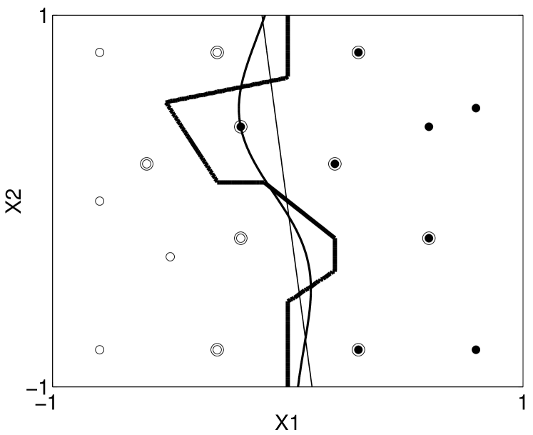
Figure 1: Illustration of the convergence of the classifier based on class-conditional Parzen window density estimation to the $1$-NN classifier in $\mathcal{O}=\left[-1,+1\right]^{2}\subset\mathbb{R}^{2}$ using $d^{2}\left(\mathbf{x},\mathbf{x}^{\prime}\right)=\left\|\mathbf{x}-\mathbf{x}^{\prime}\right\|^{2}$. For $\sigma=5$ the decision surface (thin line) is almost linear, for $\sigma=0.4$ the curved line (medium line) results, and for very small $\sigma=0.02$ the piecewise linear decision surface (thick line) of $1$-NN is approaches. For $1$-NN only the circled points contribute to the decision surface, comparable to support vectors in the SVM.

There exists an interesting relation to the Bayes optimal classifier $h_{\mathrm{Bayes}}$ that can be approximated using the Parzen window [ParzenParzen1962] kernel density estimate with kernel $k_{\sigma}$. If the objects $\boldsymbol{\mathsf{o}}\in\mathcal{O}$ are represented as vectors $\mathbf{x}_{\boldsymbol{\mathsf{o}}}\in\mathcal{X}\subseteq\mathbb{R}^{n}$, i.e. $d\left(\boldsymbol{\mathsf{o}},\boldsymbol{\mathsf{o}}^{\prime}\right)=\left\|\mathbf{x}_{\boldsymbol{\mathsf{o}}}-\mathbf{x}_{\boldsymbol{\mathsf{o}}^{\prime}}\right\|$ then the class conditional density $\boldsymbol{\mathsf{f}}_{\mathsf{X}|\mathsf{Y}=\pm 1}$ can be estimated using a Parzen window density estimator

$$\boldsymbol{\widehat{\mathsf{f}}}_{\mathsf{X}|\mathsf{Y}=\pm 1}\left(\mathbf{x}\right)=\frac{1}{m^{\pm}}\sum_{i=1}^{m^{\pm}}k_{\sigma}\left(\mathbf{x},\mathbf{x}_{\boldsymbol{\mathsf{o}}_{i}}\right)\,,$$

where the kernel is assumed to be normalised to one, i.e. $\int_{\mathcal{X}}k_{\sigma}\left(\mathbf{x}\right)\,d\mathbf{x}=1$. The Bayes optimal decision at point $\mathbf{x}$ is given by

$$h_{\mathrm{Bayes}}\left(\boldsymbol{\mathsf{o}}\right)=\textrm{sign}\left(\boldsymbol{\mathsf{f}}_{\mathsf{X}|\mathsf{Y}=+1}\left(\mathbf{x}_{\boldsymbol{\mathsf{o}}}\right)-\boldsymbol{\mathsf{f}}_{\mathsf{X}|\mathsf{Y}=-1}\left(\mathbf{x}_{\boldsymbol{\mathsf{o}}}\right)\right)$$

and can be approximated by

$$\widehat{h}_{\sigma}\left(\boldsymbol{\mathsf{o}}\right)=\textrm{sign}\left(\boldsymbol{\widehat{\mathsf{f}}}_{\mathsf{X}|\mathsf{Y}=+1}\left(\mathbf{x}_{\boldsymbol{\mathsf{o}}}\right)-\boldsymbol{\widehat{\mathsf{f}}}_{\mathsf{X}|\mathsf{Y}=-1}\left(\mathbf{x}_{\boldsymbol{\mathsf{o}}}\right)\right)\,.$$

This estimator is shown in Figure 1 for the RBF-kernel (4) and three different values of $\sigma$. The convergence $\lim_{\sigma\rightarrow 0}\widehat{h}_{\sigma}\left(\boldsymbol{\mathsf{o}}\right)=\mathrm{NN}_{1}\left(\boldsymbol{\mathsf{o}}\right)$ leads to the convergence

$$\lim_{\sigma\rightarrow 0}R\left(\widehat{h}_{\sigma}\right)=R\left(\mathrm{NN}_{1}\right)$$

on which our analysis is based. Note that the performance of $\widehat{h}_{\sigma}$ for small sample size may be bad. Also for increasing sample size $m\rightarrow\infty$ a a decreasing kernel bandwidth $\sigma\rightarrow 0$ is required for consistency.

Let us consider $k_{0}\left(\boldsymbol{\mathsf{o}},\boldsymbol{\mathsf{o}}_{i}\right)\equiv\lim_{\sigma\rightarrow 0}k_{\sigma}\left(\boldsymbol{\mathsf{o}},\boldsymbol{\mathsf{o}}_{i}\right)$ and classifiers of the form

$$g_{\boldsymbol{\alpha}}\left(\boldsymbol{\mathsf{o}}\right)=\textrm{sign}\left(\sum_{i=1}^{m}\alpha_{i}k_{0}\left(\boldsymbol{\mathsf{o}},\boldsymbol{\mathsf{o}}_{i}\right)\right)\,.$$ (5)

The $1$-NN classifier is then given by $\mathrm{NN}_{1}\left(Z,\cdot\right)=g_{\boldsymbol{\alpha}=\mathbf{y}}\equiv g_{\mathbf{y}}$, and can be expressed if we restrict the coefficients $\alpha_{i}$ to take values only from $A=\mathcal{Y}=\left\{-1,+1\right\}$. Hence, the resulting hypothesis space is given by

$$\mathcal{G}=\left\{g_{\boldsymbol{\alpha}}:\forall i\in\left\{1,\ldots,m\right\}:\alpha_{i}\in A\right\}\,.$$ (6)

It turns out that the $1$-NN classifier $g_{\mathbf{y}}$ is a minimiser of the empirical risk (1), i.e. $g_{\mathbf{y}}=\mathrm{argmin}_{g\in\mathcal{G}}\,R_{\mathrm{emp}}\left(g,Z\right)$. This is easily seen by considering that $\forall\boldsymbol{\mathsf{o}}\in O$ the $1$-neighbourhood $N_{1}\left(\boldsymbol{\mathsf{o}}\right)=\left\{\boldsymbol{\mathsf{o}}\right\}$ and thus $\forall\left(\boldsymbol{\mathsf{o}},y\right)\in Z:g_{\mathbf{y}}\left(\boldsymbol{\mathsf{o}}\right)=y$ resulting in $R_{\mathrm{emp}}\left(g_{\mathbf{y}},Z\right)=0$. Also, $g_{\mathbf{y}}\left(\boldsymbol{\mathsf{o}}\right)$ is the only minimiser of $R_{\mathrm{emp}}\left(g,Z\right)$ because for each $\alpha_{i}$ flipped, exactly one training error is incurred resulting in an increase over $R_{\mathrm{emp}}\left(g_{\mathbf{y}},Z\right)$ by $1/m$. Thus the application of $1$-NN conforms to the principle of empirical risk minimisation [VapnikVapnik1998] at vanishing training error.

Based on this view let us turn to an intuitive explanation of why the $1$-NN classifier is able to generalise. As shown in Figure 1 not all the objects $\boldsymbol{\mathsf{o}}\in O$ from the training sample $O$ contribute to the decision function. In terms of the hypothesis space defined in (5) and (6) above this means that the respective summands could be set to nought without changing the decision at any object $\boldsymbol{\mathsf{o}}\in\mathcal{O}$ . Let us define the set $\overline{Z}_{K}$ of subsets $Z^{\prime}\subset Z$ of training data redundant for the $K$-NN classifier by

$$\overline{Z}_{K}\stackrel{{\scriptstyle\mathrm{def}}}{{=}}\left\{Z^{\prime}:\forall\boldsymbol{\mathsf{o}}\in\mathcal{O}\;\mathrm{NN}_{K}\left(Z,\boldsymbol{\mathsf{o}}\right)=\mathrm{NN}_{K}\left(Z\setminus Z^{\prime},\boldsymbol{\mathsf{o}}\right)\right\},$$

and let $Z_{K}\in\overline{Z}_{K}$ be defined as the element of $\overline{Z}_{K}$ of maximum cardinality, $Z_{K}=\mathrm{argmax}_{Z^{\prime}\in\overline{Z}_{K}}\left(\left|Z^{\prime}\right|\right).$ Even if all the training examples in $Z_{K}$ were left out the prediction at no object $\boldsymbol{\mathsf{o}}\in\mathcal{O}$ would change. Please note the interesting resemblance of $Z\setminus Z_{K}$ to the set of support vectors in SVM learning [VapnikVapnik1998]. In order to be able to express this sparseness of solutions in the expansion coefficients $\alpha_{i}$ let us augment the hypothesis space $\mathcal{G}$ by allowing the coefficients $\alpha_{i}$ to take on nought as an additional value, $\forall i\in\left\{1,\ldots\,m\right\}\;\alpha_{i}\in A\cup\left\{0\right\}\equiv\widetilde{A}$. This will allow us to express prior belief in the sparseness of a solution by putting additional prior weight on solutions with few non-vanishing coefficients. The augmented hypothesis space $\widetilde{\mathcal{G}}$ is given by

$$\widetilde{\mathcal{G}}=\left\{g_{\boldsymbol{\widetilde{\alpha}}}:\alpha_{i}\in\widetilde{A}\right\}.$$ (7)

Then we can define the set $G_{\mathbf{y}}\subseteq\widetilde{\mathcal{G}}$ of hypotheses that are equivalent to $g_{\mathbf{y}}$ w.r.t. the classification on $\mathcal{O}$

$$G_{\mathbf{y}}=\left\{g_{\boldsymbol{\alpha}}\in\widetilde{\mathcal{G}}:\forall\boldsymbol{\mathsf{o}}\in\mathcal{O}\;g_{\boldsymbol{\alpha}}\left(\boldsymbol{\mathsf{o}}\right)=g_{\mathbf{y}}\left(\boldsymbol{\mathsf{o}}\right)\right\}.$$ (8)

The cardinality $\left|G_{\mathbf{y}}\right|$ of this set will later serve as the crucial quantity for bounding the generalisation error. Since the set $G_{\mathbf{y}}$ is not easily accessible we can define a subset $G_{Z_{1}}\subseteq G_{\mathbf{y}}$ by

$$G_{Z_{1}}=\left\{g_{\boldsymbol{\alpha}}\in\widetilde{\mathcal{G}}:\forall\left(\boldsymbol{\mathsf{o}}_{i},y_{i}\right)\in Z\setminus Z_{1}\quad\alpha_{i}=y_{i}\right\}.$$

The cardinality $\left|G_{Z_{1}}\right|$ of this set is then given by $\left|G_{Z_{1}}\right|=2^{r}$ and is thus trivially related to the number $r$ of redundant points. It will later serve as a convenient lower bound, $\left|G_{Z_{1}}\right|\leq\left|G_{\mathbf{y}}\right|$. The redundancy $r$ can also be viewed as a kind of luckiness in the sense of [Shawe-Taylor, Bartlett, Williamson, and AnthonyShawe-Taylor et al.1996].

5 A PAC-Bayesian bound for 1-NN

We would like to define a prior over $\widetilde{\mathcal{G}}$ and apply the PAC-Bayesian Theorem 1. However, the prior over the hypothesis space $\mathcal{H}$ as referred to in Theorem 1 requires us to define an hypothesis space $\mathcal{H}$ before learning. In contrast, the hypothesis space $\widetilde{\mathcal{G}}$ defined by equations (5) and (7) appears to be data-dependent and thus not known before the data are considered. Let us consider an alternative hypothesis space given by all the linear functions

$$\mathcal{H}=\left\{h_{\mathbf{w}}:h_{\mathbf{w}}=\mathrm{sign}\left(\left\langle\mathbf{w},\boldsymbol{\phi}\left(\boldsymbol{\mathsf{o}}\right)\right\rangle_{\mathcal{K}}\right),\mathbf{w}\in\mathcal{K},\left\|\mathbf{w}\right\|_{\mathcal{K}}=1\right\}.$$

$\mathcal{K}$ is the kernel space associated with the kernel

$$k_{\sigma}\left(\boldsymbol{\mathsf{o}},\boldsymbol{\mathsf{o}}^{\prime}\right)=\left\langle\boldsymbol{\phi}\left(\boldsymbol{\mathsf{o}}\right),\boldsymbol{\phi}\left(\boldsymbol{\mathsf{o}}^{\prime}\right)\right\rangle_{\mathcal{K}},$$

and $\boldsymbol{\phi}:\mathcal{O}\mapsto\mathcal{K}$. The unit length constraint $\left\|\mathbf{w}\right\|_{\mathcal{K}}=1$ is required in order to be able to define a proper (normaliseable) prior measure over $\mathcal{H}_{\mathbf{w}}$ such that $\boldsymbol{\mathsf{P}}_{\mathsf{H}_{\mathbf{w}}}\left(\mathcal{H}_{\mathbf{w}}\right)=1$. Since we can expand the weight vector $\mathbf{w}$ in terms of the objects $\boldsymbol{\mathsf{o}}_{i}\in Z$ by

$$\mathbf{w}=\sum_{i=1}^{m}\alpha_{i}\boldsymbol{\phi}\left(\boldsymbol{\mathsf{o}}_{i}\right)$$ (9)

the hypotheses as given in equation (5) can be written as

$$g_{\boldsymbol{\alpha}}\left(\boldsymbol{\mathsf{o}}\right) = \mathrm{sign}\left(\sum_{i=1}^{m}\alpha_{i}k_{\sigma}\left(\boldsymbol{\mathsf{o}},\boldsymbol{\mathsf{o}}_{i}\right)\right)$$

$$= \mathrm{sign}\left(\sum_{i=1}^{m}\alpha_{i}\left\langle\boldsymbol{\phi}\left(\boldsymbol{\mathsf{o}}_{i}\right),\boldsymbol{\phi}\left(\boldsymbol{\mathsf{o}}\right)\right\rangle_{\mathcal{K}}\right)$$

$$= \mathrm{sign}\left(\left\langle\mathbf{w},\boldsymbol{\phi}\left(\boldsymbol{\mathsf{o}}\right)\right\rangle_{\mathcal{K}}\right)$$

$$= h_{\mathbf{w}}\left(\boldsymbol{\mathsf{o}}\right)$$

Thus for every hypothesis $g_{\boldsymbol{\alpha}}\in\widetilde{\mathcal{G}}$ there exists a corresponding hypothesis $h_{\mathbf{w}}\in\mathcal{H}$ before the training data $Z$ are considered. Since Theorem 1 holds for any two probability measures $\boldsymbol{\mathsf{P}}_{\mathsf{H}}$ and $\boldsymbol{\mathsf{P}}_{\mathsf{OY}}$ it is sufficient to show that given any prior measure $\boldsymbol{\mathsf{P}}_{\widetilde{\mathsf{G}}}$ over $\widetilde{\mathcal{G}}$ there always exists a corresponding prior measure $\boldsymbol{\mathsf{P}}_{\mathsf{H}}$ over $\mathcal{H}$.

Let us define the $\left(\dim\left(\mathcal{K}\right)\times m\right)$-matrix

$$\boldsymbol{\Phi}\left(O\right)=\left(\boldsymbol{\phi}\left(\boldsymbol{\mathsf{o}}_{1}\right),\ldots,\boldsymbol{\phi}\left(\boldsymbol{\mathsf{o}}_{m}\right)\right)$$

of training objects $\boldsymbol{\mathsf{o}}$ mapped to kernel space $\mathcal{K}$. Then the linear transformation from the parameter space $\widetilde{A}^{m}$ to kernel space $\mathcal{K}$ can be written as $\mathbf{w}=\boldsymbol{\Phi}\left(O\right)\boldsymbol{\alpha}$ and we have for any measurable subset $H\subseteq\mathcal{H}$ a corresponding set $\widetilde{G}\subseteq\widetilde{\mathcal{G}}$ given by

$$\widetilde{G}\left(H,O\right)=\left\{g_{\boldsymbol{\alpha}}:\exists\mathbf{w}\in H\quad\frac{\boldsymbol{\Phi}\left(O\right)\boldsymbol{\alpha}}{\left\|\boldsymbol{\Phi}\left(O\right)\boldsymbol{\alpha}\right\|}=\mathbf{w}\right\}$$

The resulting prior measure $\boldsymbol{\mathsf{P}}_{\mathsf{H}}$ is given by

$$\boldsymbol{\mathsf{P}}_{\mathsf{H}}\left(H\right)=\boldsymbol{\mathsf{E}}_{\mathsf{O}^{m}}\left[\boldsymbol{\mathsf{P}}_{\widetilde{\mathsf{G}}}\left(\widetilde{G}\left(H,\mathsf{O}\right)\right)\right],$$

indicating that knowledge of the measure $\boldsymbol{\mathsf{P}}_{\mathsf{O}}$ over objects is necessary in order to determine $\boldsymbol{\mathsf{P}}_{\mathsf{H}}$. This does not constitute a problem, however, because explicit knowledge of $\boldsymbol{\mathsf{P}}_{\mathsf{H}}$ is neither required for the application of the algorithm nor for the calculation of the PAC-Bayesian bound values.

First, let us illustrate the application of the PAC-Bayesian bound (1) by constructing a very simple prior $\boldsymbol{\mathsf{P}}_{\widetilde{\mathsf{G}}}\left(\boldsymbol{\alpha}\right)$ over $\widetilde{\mathcal{G}}$. Due to the iid property of the training sample $Z$, we have no knowledge about any specific $\alpha_{i}$ and thus choose a factorising prior

$$\boldsymbol{\mathsf{P}}_{\widetilde{\mathsf{G}}}\left(g_{\boldsymbol{\alpha}}\right)=\prod_{i=1}^{m}\boldsymbol{\mathsf{P}}_{\widetilde{\mathsf{A}}}\left(\alpha_{i}\right),$$ (10)

that reflects the interchangeability of the training examples in $Z$. Assuming no further knowledge about the plausibility of hypotheses let us choose the prior to be uniform,

$$\boldsymbol{\mathsf{P}}_{\widetilde{\mathsf{A}}=-1}\left(\alpha_{i}\right)=\boldsymbol{\mathsf{P}}_{\widetilde{\mathsf{A}}=1}\left(\alpha_{i}\right)=\boldsymbol{\mathsf{P}}_{\widetilde{\mathsf{A}}=0}\left(\alpha_{i}\right)=\frac{1}{3},$$

which obviously leads to a uniform measure $\boldsymbol{\mathsf{P}}_{\widetilde{\mathsf{G}}}\left(\boldsymbol{\alpha}\right)$, as well. This choice will later be refined in the light of general knowledge about the sparseness of typical $1$-NN classifiers. Then the measure of hypotheses $g_{\boldsymbol{\alpha}}\in G_{\mathbf{y}}$ equivalent to $g_{\mathbf{y}}$ on $\mathcal{O}$ is given by

$$\boldsymbol{\mathsf{P}}_{\widetilde{\mathsf{G}}}\left(G_{\mathbf{y}}\right)=\frac{\left|G_{\mathbf{y}}\right|}{\left|\widetilde{\mathcal{G}}\right|}\geq\frac{\left|G_{Z_{1}}\right|}{\left|\widetilde{\mathcal{G}}\right|}=\frac{2^{r}}{3^{m}-1},$$ (11)

because among the total of $3^{m}-1$ hypotheses in $\widetilde{\mathcal{G}}$ we have $2^{r}$ hypotheses that agree with $g_{\mathbf{y}}$ on $\mathcal{O}$. Then we can give the following bound on the generalisation error of $1$-NN.

Theorem 3.

For any probability distribution $\boldsymbol{\mathsf{P}}_{\mathsf{Z}}$ on labelled objects we have, for any $\delta>0,$ that with probability at least $1-\delta$ over the selection of a sample of $m$ examples, the following holds for the $1$-NN classifier $g_{\mathbf{y}}$ with $r$ redundant examples :

$$R\left(g_{\mathbf{y}}\right)\leq\frac{m\log 3-r\log 2+\log\frac{1}{\delta}}{m}.$$

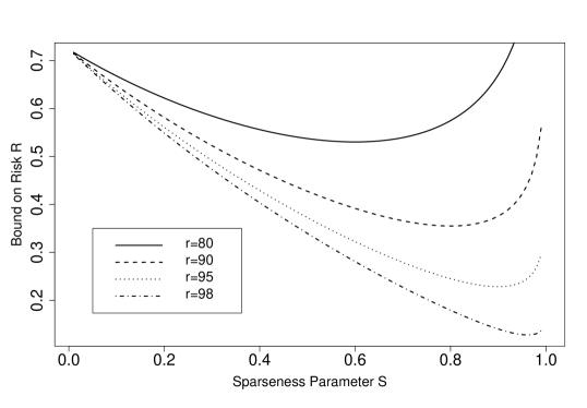
Figure 2: Values of the bound given in Theorem 4 as a function of the expected sparsity $S$ for four different values $r$ of the observed number of redundant objects. The training set size is $m=100$ and the confidence is $95\%$ corresponding to $\delta=0.05$. Large values of $r$ lead to lower values of the bound, but the bound attains its minimum only if the expected sparsity $S$ matches the the number of redundant objects $r$. Note that the optimum $S_{\mathrm{opt}}$ for a given redundancy $r$ is $S_{\mathrm{opt}}<\frac{r}{m}$, the value one may have expected.

Let us refine this bound by constructing a more informative prior $\boldsymbol{\mathsf{P}}_{\widetilde{\mathsf{G}}}$. Maintaining the factorising property (10) and introducing an expected level $S$ of sparsity we choose

$$\boldsymbol{\mathsf{P}}_{\widetilde{\mathsf{A}}=0}\left(\alpha_{i}\right)=S\;\mathrm{and}\;\boldsymbol{\mathsf{P}}_{\widetilde{\mathsf{A}}=-1}\left(\alpha_{i}\right)=\boldsymbol{\mathsf{P}}_{\widetilde{\mathsf{A}}=1}\left(\alpha_{i}\right)=\frac{1-S}{2}$$

The resulting prior measure $\boldsymbol{\mathsf{P}}_{\widetilde{\mathsf{G}}}$ is then only a function of the sparsity $s\left(g_{\boldsymbol{\alpha}}\right)$ of an hypothesis $g_{\boldsymbol{\alpha}}$ given by $s\left(g_{\boldsymbol{\alpha}}\right)=\left|\left\{i\in\left\{1,\ldots\,m\right\}:\alpha_{i}=0\right\}\right|$. We are interested in the prior measure $\boldsymbol{\mathsf{P}}_{\widetilde{\mathsf{G}}}\left(G_{\mathbf{y}}\right)$ of all those hypotheses $g_{\boldsymbol{\alpha}}\in\widetilde{\mathcal{G}}$ that behave equivalently to $g_{\mathbf{y}}$ on $\mathcal{O}$. This quantity is lower bounded by $\boldsymbol{\mathsf{P}}_{\widetilde{\mathsf{G}}}\left(G_{Z_{1}}\right)$.

$$\boldsymbol{\mathsf{P}}_{\widetilde{\mathsf{G}}}\left(G_{Z_{r}}\right) = \sum_{s=0}^{r}\left(\begin{array}[]{c}r\\ s\end{array}\right)\frac{S^{s}\left(\frac{1-S}{2}\right)^{m-s}}{1-S^{m}}$$ (14)

$$= \frac{\left(\frac{1-S}{2}\right)^{m-r}}{1-S^{m}}\sum_{s=0}^{r}\left(\begin{array}[]{c}r\\ s\end{array}\right)S^{s}\left(\frac{1-S}{2}\right)^{r-s}$$

$$= \frac{\left(\frac{1-S}{2}\right)^{m-r}\left(\frac{1}{2}\left(1+S\right)\right)^{r}}{1-S^{m}}$$

$$= \frac{\left(1-S\right)^{m-r}\left(1+S\right)^{r}}{2^{m}\left(1-S^{m}\right)}.$$ (18)

Note, that this reduces to the previous result (11) for $S=1/3.$ Using the result (18) we can give a more refined PAC-Bayesian bound on the generalisation error of $1$-NN.

Theorem 4.

For any distribution $\boldsymbol{\mathsf{P}}_{\mathsf{Z}}$ over labelled objects and any sparsity value $S\in\left[0,1\right[$ chosen a-priori, we have, for any $\delta>0,$ that with probability at least $1-\delta$ over the selection of a sample of $m$ examples, the following holds for the $1$-NN classifier $g_{\mathbf{y}}$ with $r$ redundant examples :

$$R\left(g_{\mathbf{y}}\right)\leq\frac{m\log\frac{2\left(1-S^{m}\right)}{\left(1-S\right)}+r\log\frac{\left(1-S\right)}{\left(1+S\right)}+\log\frac{1}{\delta}}{m}.$$

In order to get a feel for the bound, consider first Figure 2. The convex shapes of the curves clearly indicate that a wrong choice of $S$ hurts in both cases: For over- and underestimated redundancy. Figure 3 illustrates the behaviour of the bound as a function of redundancy $r$. The case $S=0$ effectively corresponds to the unaugmented hypothesis space $\mathcal{G}$ with a flat prior. Due to the increase $\left|\mathcal{G}\right|=2^{m}$ of $\mathcal{G}$ with $m$ the resulting cardinality bound can never give values below $\sqrt{2}\approx 0.69$. The case $S=0.33$ corresponds to the bound of Theorem 3 and is superior mostly in “trivial” regimes with $R>0.5$. Only for “courageous” choices of $S=0.9$ and $S=0.99$ does the bound reach non-trivial regimes. It should be noted that standard VC-bounds often require training set sizes of $m>100000$ for even the luckiest cases to give non-trivial bounds ($R<0.5$).

As a matter of fact, it is feasible to incorporate even more knowledge than the level of sparsity $S$ into the bound. In addition, knowledge about the a-priori class probabilities $\boldsymbol{\mathsf{P}}_{\mathsf{Y}}\left(\mathsf{Y}=\pm 1\right)$ and knowledge about the levels of sparsity $S^{\pm}$ in each of the classes could be incorporated in the bound.

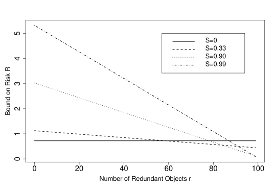
Figure 3: Values of the bound given in Theorem 4 as a function of the number $r$ of redundant objects for four different values of the expected sparsity $S$. The training set size is $m=100$ and the confidence is $95\%$ corresponding to $\delta=0.05$. Large values of $S$ lead to lower values of the bound, but only for sufficiently large values of $r$. If the value of $S$ is chosen too optimistically, the resulting value of the bound suffers.

6 The general case of $K$-NN

In practice, people often use the $K$-NN classifier, $K>1$, rather than the $1$-NN classifier to avoid over-fitting the data. In order to arrive at a similar result as that obtained in Section 5 let us find a formulation for $K$-NN equivalent to that given in (3) for $1$-NN. We avoid the problem of voting ties by considering only odd values of $K$. Since the $K$ nearest neighbours need to be selected, we use a product of kernels,

$$\mathrm{NN}_{K}\left(Z,\boldsymbol{\mathsf{o}}\right) = \mathrm{sign}\left(\sum_{\stackrel{{\scriptstyle\left(\boldsymbol{\mathsf{o}}^{\prime},y^{\prime}\right)\in Z:}}{{\boldsymbol{\mathsf{o}}^{\prime}\in N_{K}(\boldsymbol{\mathsf{o}})}}}y^{\prime}\right)$$ (19)

$$= \mathrm{sign}\left(\sum_{\stackrel{{\scriptstyle Z^{\prime}\subseteq Z:}}{{\left|Z^{\prime}\right|=K}}}\prod_{Z^{\prime}}k_{0}\left(\boldsymbol{\mathsf{o}},\boldsymbol{\mathsf{o}}^{\prime}\right)\sum_{Z^{\prime}}^{K}y^{\prime}\right)$$

$$= \mathrm{sign}\left(\sum_{\mathbf{i}\in I}\prod_{j=1}^{K}k_{0}\left(\boldsymbol{\mathsf{o}},\boldsymbol{\mathsf{o}}_{i_{j}}\right)\sum_{l=1}^{K}y_{i_{l}}\right).$$

The sum is over the set $I$ of index vectors $\mathbf{i}\in I$ defined as

$$I\equiv\left\{\mathbf{i}\in\left\{1,\ldots,m\right\}^{K}:\forall j\in\left\{1,\ldots,m-1\right\}\>i_{j+1}>i_{j}\right\},$$

and we use components $i_{j}$ of $\mathbf{i}=\left(i_{1},\ldots,i_{K}\right)^{\prime}$ for indexing. Again the above classifier can be considered a linear classifier in a kernel space if we define an augmented product kernel $\widetilde{k}:\mathcal{O}^{K}\times\mathcal{O}^{K}\mapsto\mathbb{R}^{+}$by

$$\widetilde{k}\left(\boldsymbol{\mathsf{o}}_{1},\ldots\,\boldsymbol{\mathsf{o}}_{K},\boldsymbol{\mathsf{o}}_{K+1},\ldots,\boldsymbol{\mathsf{o}}_{2K}\right)\equiv\prod_{j=1}^{K}k\left(\boldsymbol{\mathsf{o}}_{j},\boldsymbol{\mathsf{o}}_{j+K}\right).$$

The product kernel $\widetilde{k}$ retains its Mercer property due to the closure of kernels under the tensor product [HausslerHaussler1999]. Defining coefficients $\beta_{\mathbf{i}}\equiv\sum_{l=1}^{K}\alpha_{i_{l}}$ with $\forall i\in\left\{1,\ldots,m\right\}\>\alpha_{i}=y_{i}$ we express the $K$-NN classifier as the limiting case of a linear classifier

$$\mathrm{NN}_{K}\left(Z,\boldsymbol{\mathsf{o}}\right)=\mathrm{sign}\left(\sum_{\mathbf{i}\in I}\beta_{\mathbf{i}}\widetilde{k}_{0}(\underbrace{\boldsymbol{\mathsf{o}},\ldots,\boldsymbol{\mathsf{o}}}_{K\,\mathrm{times}},\boldsymbol{\mathsf{o}}_{i_{1}},\ldots,\boldsymbol{\mathsf{o}}_{i_{j}})\right).$$

Since the coefficients $\beta_{\mathbf{i}}=\beta_{\mathbf{i}}\left(\boldsymbol{\alpha}\right)$ are fully determined by the values of the $\alpha_{i}$ it is sufficient to consider these. As discussed in Section 4 the $1$-NN classifier can be considered as the empirical risk minimiser with vanishing training error. The situation is different for $K$-NN. Consider, e.g. the situation of a training sample of three different objects two of which belong to one class and one of which belongs to the other class. For $K=3$ under any metric the $3$-NN classifier will incur a loss of $1/3$ because the single object belonging to the minority class will be classified as belonging to the majority class.

Again we can use the redundancy of features to benefit from sparse solutions in the coefficients $\alpha_{i}$. As in the case of $1$-NN the two types of results as in Theorems 3 and 4 are possible, this time base on Theorem 2. We will give here only the version corresponding to Theorem 4 because Theorem 3 follows as a special case thereof.

Theorem 5.

For any probability distribution $\boldsymbol{\mathsf{P}}_{\mathsf{Z}}$ on labelled objects and any sparsity value $S\in\left[0,1\right[$ chosen a-priori, we have, for any $\delta>0,$ that with probability at least $1-\delta$ over the selection of a sample of $m$ examples, the following holds for the $K$-NN classifier $g_{\mathbf{y}}^{K}$ with $r_{K}=\log_{2}\left|G_{Z_{K}}\right|$ redundant examples: The difference

$$\Delta R=R\left(g_{\mathbf{y}}^{K}\right)-R_{\mathrm{emp}}\left(g_{\mathbf{y}}^{K};Z\right)$$

between actual and empirical risk is bounded from above by

$$\Delta R\leq\sqrt{\frac{m\log\frac{2\left(1-S^{m}\right)}{\left(1-S\right)}+r_{K}\log\frac{\left(1-S\right)}{\left(1+S\right)}+\log\frac{1}{\delta}}{2m}}.$$

While this bound behaves similarly to the one given in Theorem 4 in terms of $r_{K}$ and $S$, it is more interesting to ask about the dependency of $\left|G_{\mathbf{y}}\right|$ (or its lower bound $2^{r_{K}}$) on the number $K$ of neighbours considered. Empirical results indicate that the risk $R(g_{\mathbf{y}}^{K})$ is a bowl-shaped function of $K$, indicating the existence of an optimum number $K>1$. A corresponding theoretical result together with Theorem would then yield a sound explanation of why $K>1$ may be preferred, and may even serve as a guide for model selection.

7 Conclusions and Future Work

We provided small sample size bounds on the generalisation error of the $K$-nearest-neighbour classifier in the PAC-Bayesian framework by viewing $K$-NN as a linear classifier in a collapsed kernel space. Referring back to the goal set in the Introduction these bounds may serve to make $K$-NN a self-bounding algorithm in the sense of [FreundFreund1998]. It is left for future research to provide means for determining in practice at least an estimate of the number $r_{K}$ of redundant points.

Interestingly, our analysis involves the notion of redundant examples and — as a consequence — of essential examples that bear a close resemblance with support vectors [VapnikVapnik1998]. Also, considering Figure 1 it is obvious that $1$-NN performs a local margin maximisation as opposed to a global margin maximisation in the SVM.

Pursuing the similarity to SVMs further, note that the $K$-NN classifier not only returns a classification for a given object $\boldsymbol{\mathsf{o}}\in\mathcal{O}$, but also provides a discrete margin

$$\gamma\left(\boldsymbol{\mathsf{o}}\right)=y\sum_{i:\boldsymbol{\mathsf{o}}_{i}\in N_{K}(\boldsymbol{\mathsf{o}})}y_{i}$$

taking values $\gamma\in\left\{-K,-K+2,\ldots,K-2,K\right\}$. Hence, we can define the margin $\gamma_{Z}$ on the training sample $Z$ by $\gamma_{Z}=\min_{\left(\boldsymbol{\mathsf{o}},y\right)\in Z}\gamma\left(\boldsymbol{\mathsf{o}}\right).$ Since the now famous Support Vector Machine [VapnikVapnik1998] is based on maximising the margin and also generalisation bounds for linear classifiers [Herbrich, Graepel, and CampbellHerbrich et al.1999, VapnikVapnik1998] are based on this notion it is tempting to speculate that also for $K$-NN the margin $\gamma_{Z}$ on the training sample should play a role in the generalisation bound. Intuitively, the relation between $\left|G_{\mathbf{y}}\right|$ and the margin $\gamma_{Z}$ is clear: The more unanimous the outcome of the voting on $O$ the more hypotheses $g_{\boldsymbol{\alpha}}\in\widetilde{\mathcal{G}}$ would give the same classification of the training data and therefore more likely agree on $\mathcal{O}$. However, at this point it is not clear how exactly the margin $\gamma_{Z}$ is related to $\left|G_{\mathbf{y}}\right|$, the quantity determining generalisation.

Another interesting aspect of the margin $\gamma\left(\boldsymbol{\mathsf{o}}\right)$ is its use as a confidence measure for the prediction of labels on test objects. For linear classifiers this method has been theoretically justified by [Shawe-TaylorShawe-Taylor1996]. Indeed, for $K$-NN such a strategy has been put forward in the form of the $\left(K,L\right)$-nearest-neighbour rule [HellmanHellman1970] that given a parameter $L>K/2$ refuses to make predictions at $\boldsymbol{\mathsf{o}}$ unless $\gamma\left(\boldsymbol{\mathsf{o}}\right)\geq L$. Depending on $L$ this principle leads to a rejection rate $\rho\left(L\right)$ on a given test sample. Based on $L$ and $\rho\left(L\right)$ it should be possible to bound the risk on the non-rejected points.

References

• [\citeauthoryearDevroye, Gyรถrfi, and LugosiDevroye etย al.1996] Devroye, L., L.ย Gyรถrfi, and G.ย Lugosi (1996). A Probabilistic Theory of Pattern Recognition. Numberย 31 in Applications of mathematics. New York: Springer.
• [\citeauthoryearFix and HodgesFix and Hodges1951a] Fix, E. and J.ย Hodges (1951a). Discriminatory analysis. nonparametric discrimination: Consistency properties. Technical report, USAF School of Aviation Medicine. Technical Report 21-49-004.
• [\citeauthoryearFix and HodgesFix and Hodges1951b] Fix, E. and J.ย Hodges (1951b). Discriminatory analysis: small sample performance. Technical report, USAF School of Aviation Medicine. Technical Report 21-49-004.
• [\citeauthoryearFreundFreund1998] Freund, Y. (1998). Self bounding learning algorithms. In Proceedings of the Annual Conference on Computational Learning Theory, Madison, Wisconsin, pp.ย  247โ€“258.
• [\citeauthoryearHausslerHaussler1999] Haussler, D. (1999). Convolutional kernels on discrete structures. Technical Report UCSC-CRL-99-10, Computer Science Department, University of California at Santa Cruz.
• [\citeauthoryearHellmanHellman1970] Hellman, M.ย E. (1970). The nearest neighbor classification rule with a reject option. IEEE Transactions on Systems Science and Cyberneticsย 6(3), 179โ€“185.
• [\citeauthoryearHerbrich, Graepel, and CampbellHerbrich etย al.1999] Herbrich, R., T.ย Graepel, and C.ย Campbell (1999). Bayes point machines: Estimating the Bayes point in kernel space. In Proceedings of IJCAI Workshop Support Vector Machines, pp.ย 23โ€“27.
• [\citeauthoryearMcAllesterMcAllester1998] McAllester, D.ย A. (1998). Some PAC Bayesian theorems. In Proceedings of the Annual Conference on Computational Learning Theory, Madison, Wisconsin, pp.ย  230โ€“234. ACM Press.
• [\citeauthoryearMercerMercer1909] Mercer, T. (1909). Functions of positive and negative type and their connection with the theory of integral equations. Transaction of London Philosophy Society (A)ย 209, 415โ€“446.
• [\citeauthoryearParzenParzen1962] Parzen, E. (1962). On estimation of probability density function and mode. Annals of Mathematical Statisticsย 33(3), 1065โ€“1076.
• [\citeauthoryearShawe-TaylorShawe-Taylor1996] Shawe-Taylor, J. (1996). Confidence estimates of classification accuracy on new examples. Technical report, Royal Holloway, University of London. NC2-TR-1996-054.
• [\citeauthoryearShawe-Taylor, Bartlett, Williamson, and AnthonyShawe-Taylor etย al.1996] Shawe-Taylor, J., P.ย L. Bartlett, R.ย C. Williamson, and M.ย Anthony (1996). Structural risk minimization over dataโ€“dependent hierarchies. Technical report, Royal Holloway, University of London. NCโ€“TRโ€“1996โ€“053.
• [\citeauthoryearVapnikVapnik1998] Vapnik, V. (1998). Statistical Learning Theory. New York: John Wiley and Sons.
• [\citeauthoryearWolpertWolpert1995] Wolpert, D.ย H. (1995). The Mathematics of Generalization, Chapter 3,The Relationship between PAC, the Statistical Physics Framework, the Bayesian Framework, and the VC framework, pp.ย  117โ€“215. Addison Wesley.