Zee-Babu model in modular $A_{4}$ symmetry

Abstract

We study a Zee-Babu model in a modular $A_{4}$ flavor symmetry, in which we search for several predictions such as phases, sum of neutrino masses, and neutrinoless double beta decay, satisfying neutrino oscillation data in a minimum framework of the charge assignments of modular weight. We perform $\Delta\chi^{2}$ analysis to get our results and find $\tau$ is localized nearby at one of the fixed points of $i\times\infty$ for both of normal and inverted mass hierarchies.

I Introduction

Zee-Babu model is one of the attractive scenarios to get active neutrino matrix at two-level, since only one singly- and one doubly-charged bosons are introduced in the standard model(SM) without any additional symmetries Zee-Babu . Also the neutrino mass matrix depends on structure of the charged-lepton mass matrix. Thus, it has a lot of interesting phenomenologies that should be taken in account; e.g., lepton flavor universalities Babu:2002uu , lepton flavor violations Babu:2002uu ; AristizabalSierra:2006gb , collider physics at Large Hadron Collider for new charged-bosons Schmidt:2014zoa ; Nebot:2007bc . The model has a unique prediction for lepton sector that one of the lightest neutrino masses is always zero because the mass matrix consists of three by three anti-symmetric matrix whose rank is two. However, there still exist too many free parameters to get further predictions such as CP phases and mixing patterns in the lepton sector.

A few years ago, an attractive flavor symmetry has been proposed by papers Feruglio:2017spp ; deAdelhartToorop:2011re , in which they have applied a non-Abelian discrete flavor symmetry originated by a modular symmetry in order to find further predictions for quark and lepton sectors without introducing so many bosons. Along the line of this idea, a vast reference has recently appeared in the literature, e.g., $A_{4}$ Feruglio:2017spp ; Criado:2018thu ; Kobayashi:2018scp ; Okada:2018yrn ; Nomura:2019jxj ; Okada:2019uoy ; deAnda:2018ecu ; Novichkov:2018yse ; Nomura:2019yft ; Okada:2019mjf ; Ding:2019zxk ; Nomura:2019lnr ; Kobayashi:2019xvz ; Asaka:2019vev ; Zhang:2019ngf ; Gui-JunDing:2019wap ; Kobayashi:2019gtp ; Nomura:2019xsb ; Wang:2019xbo ; Okada:2020dmb ; Okada:2020rjb ; Behera:2020lpd ; Behera:2020sfe ; Nomura:2020opk ; Nomura:2020cog ; Asaka:2020tmo ; Okada:2020ukr ; Nagao:2020snm ; Okada:2020brs ; Yao:2020qyy ; Chen:2021zty ; Kashav:2021zir ; Okada:2021qdf ; deMedeirosVarzielas:2021pug ; Nomura:2021yjb ; Hutauruk:2020xtk ; Ding:2021eva ; Nagao:2021rio ; king , $S_{3}$ Kobayashi:2018vbk ; Kobayashi:2018wkl ; Kobayashi:2019rzp ; Okada:2019xqk ; Mishra:2020gxg ; Du:2020ylx , $S_{4}$ Penedo:2018nmg ; Novichkov:2018ovf ; Kobayashi:2019mna ; King:2019vhv ; Okada:2019lzv ; Criado:2019tzk ; Wang:2019ovr ; Zhao:2021jxg ; King:2021fhl ; Ding:2021zbg ; Zhang:2021olk ; gui-jun ; Nomura:2021ewm , $A_{5}$ Novichkov:2018nkm ; Ding:2019xna ; Criado:2019tzk , double covering of $A_{5}$ Wang:2020lxk ; Yao:2020zml ; Wang:2021mkw ; Behera:2021eut , larger groups Baur:2019kwi , multiple modular symmetries deMedeirosVarzielas:2019cyj , and double covering of $A_{4}$ Liu:2019khw ; Chen:2020udk ; Li:2021buv , $S_{4}$ Novichkov:2020eep ; Liu:2020akv , and the other types of groups Kikuchi:2020nxn ; Almumin:2021fbk ; Ding:2021iqp ; Feruglio:2021dte ; Kikuchi:2021ogn ; Novichkov:2021evw in which masses, mixing, and CP phases for the quark and/or lepton have been predicted . Moreover, a systematic approach to understanding the origin of CP transformations has been discussed in Ref. Baur:2019iai , and CP/flavor violation in models with modular symmetry was discussed in Refs. Kobayashi:2019uyt ; Novichkov:2019sqv , and a possible correction from Kähler potential was discussed in Ref. Chen:2019ewa . Furthermore, systematic analysis of the fixed points (stabilizers) has been discussed in Ref. deMedeirosVarzielas:2020kji .

In this paper, we study a Zee-Babu model imposing the modular $A_{4}$ symmetry, in which we further search for predictions from this symmetry. We perform $\Delta\chi^{2}$ analysis to get our results and show several predictions for both of the normal and inverted hierarchies.

This paper is organized as follows. In Sec. II, we review our model, constructing the valid Yukawa Lagrangian, Higgs potential, charged-lepton mass matrix, and neutrino mass matrix. In neutrino sector, we show several relations coming from features of Zee-Babu model and modular $A_{4}$ symmetry. Then, we perform the $\Delta\chi^{2}$ analysis to get our results, considering their theoretical origin. We have conclusions and discussion in Sec. III. In Appendix, we show helpful formalisms on the neutrino masses and mixings, and the modular symmetry.

	Leptons
	$[\bar{L}_{L_{e}},\bar{L}_{L_{\mu}},\bar{L}_{L_{\tau}}]$	$\ell_{R}$
$SU(2)_{L}$	$\bm{2}$	$\bm{1}$
$U(1)_{Y}$	$\frac{1}{2}$	$-1$
$A_{4}$	$[1,1^{\prime\prime},1^{\prime}]$	$3$
$-k_{I}$	$[-2,-4,-6]$	$0$

Table 1: Lepton contents and their charge assignments in Zee-Babu model under $SU(2)_{L}\times U(1)_{Y}\times A_{4}$ where $-k_{I}$ is the number of modular weight and $\ell_{R}\equiv[e_{R},\mu_{R},\tau_{R}]^{T}$.

II Model

	$H$	${s^{-}}$	$k^{++}$
$SU(2)_{L}$	$\bm{2}$	$\bm{1}$	$\bm{1}$
$U(1)_{Y}$	$\frac{1}{2}$	$1$	$2$
$A_{4}$	$\bm{1}$	$\bm{1}$	$\bm{1}$
$-k_{I}$	$0$	$-4$	$0$

Table 2: Charge assignments for boson sector in Zee-Babu model under $SU(2)_{L}\times U(1)_{Y}$.

II.1 Model setup

Here, we review Zee-Babu mode, and assigning charges under the symmetries of $SU(2)_{L}\times U(1)_{Y}\times A_{4}\times(-k)$ into the lepton and Higgs sectors where $SU(3)_{c}$ is singlet for any exotic fields. As for the fermion sector, no new fields are introduced. In the SM fermions, the left-handed leptons, which are denoted by $\bar{L}_{L}\equiv[\bar{L}_{L_{e}},\bar{L}_{L_{\mu}},\bar{L}_{L_{\tau}}]$, are respectively assigned to be $[1,1^{\prime\prime},1^{\prime}]$ under $A_{4}$ with $[-2,-4,-6]$ modular weight , while right-handed charged-leptons symbolized by $\ell_{R}\equiv[e_{R},\mu_{R},\tau_{R}]^{T}$ are assigned to be triplet under $A_{4}$ with zero modular weight. The fermionic contents and their charged assignments are shown in Table 1.

In the boson sector, we introduce a singly-charged scalar $s^{-}$ with $-4$ modular weight, and a doubly-charged singlet one $k^{++}$ with zero modular weight, where all the bosons including SM Higgs $H$ are assigned to be trivial singlet $1$ under $A_{4}$. $s^{-}$ and $k^{++}$ play an role in generating the Zee-Babu two-loop neutrino mass matrix. The SM Higgs is defined by $H=[h^{+},(v_{H}+h_{0}+iz)/\sqrt{2}]^{T}$, where $h^{+}$ and $z$ are absorbed by the SM gauge bosons $W^{+}$ and $Z$, respectively and $v_{H}$ is 246 GeV. The bosonic field contents and their charge assignments are listed in Table 2. Under these symmetries, we find the valid renormalizable Lagrangian as follows:

$$-\mathcal{L}_{Y} =a_{\ell}\bar{L}_{L_{e}}H(y_{1}e_{R}+y_{2}\tau_{R}+y_{3}\mu_{R})+b_{\ell}\bar{L}_{L_{\mu}}H(y_{3}^{(4)}\tau_{R}+y_{1}^{(4)}\mu_{R}+y_{2}^{(4)}e_{R})$$

$$+c_{\ell}\bar{L}_{L_{\tau}}H(y_{2}^{(6)}\mu_{R}+y_{1}^{(6)}\tau_{R}+y_{3}^{(6)}e_{R})+d_{\ell}\bar{L}_{L_{\tau}}H(y_{2}^{{}^{\prime}(6)}\mu_{R}+y_{1}^{{}^{\prime}(6)}\tau_{R}+y_{3}^{{}^{\prime}(6)}e_{R})$$

$$+a\bar{L}_{L_{e}}(i\sigma_{2})L^{C}_{L_{\mu}}s^{-}+b\bar{L}_{L_{e}}(i\sigma_{2})L^{C}_{L_{\tau}}s^{-}+c\bar{L}_{L_{\mu}}(i\sigma_{2})L^{C}_{L_{\tau}}s^{-}$$

$$+g(\bar{e}^{C}_{R}e_{R}+\bar{\mu}^{C}_{R}\tau_{R}+\bar{\tau}^{C}_{R}\mu_{R})k^{++}+{\rm h.c.},$$ (II.1)

where $Y^{(2)}_{3}\equiv[y_{1},y_{2},y_{3}]^{T}$, $Y^{(4)}_{3}\equiv[y_{1}^{(4)},y_{2}^{(4)},y_{3}^{(4)}]^{T}$, $Y^{(6)}_{3}\equiv[y_{1}^{(6)},y_{2}^{(6)},y_{3}^{(6)}]^{T}$, $Y^{{}^{\prime}(6)}_{3}\equiv[y_{1}^{{}^{\prime}(6)},y_{2}^{{}^{\prime}(6)},y_{3}^{{}^{\prime}(6)}]^{T}$ , $a\equiv a^{\prime}Y^{(10)}_{1^{\prime}}$, $b\equiv b^{\prime}Y^{(12)}_{1^{\prime\prime}}$, $c\equiv c^{\prime}Y^{(14)}_{1}$, and $\sigma_{2}$ is the second component of the Pauli matrix. Notice here that we have five real parameters; $a_{\ell},b_{\ell},c_{\ell},a,g$ and the three complex ones; $d_{\ell},b,c$ after phase redefinition of fields without loss of generality in the Yukawa sector. $a_{\ell},b_{\ell},c_{\ell}$ are determined in order to fix the masses of charged-lepton. To realize the anti-symmetric terms $\bar{L}_{L}(i\sigma_{2})L^{C}_{L}s^{-}$, Yukawas with modular weight 8 is minimally requested. This is because it appears three independent nonzero singlets $1,1^{\prime},1^{\prime\prime}$ as the minimum modular weight. The non-trivial terms in Higgs potential is given by

$${\cal V} =\mu s^{-}s^{-}k^{++}+{\cal V}_{2}^{tri}+{\cal V}_{4}^{tri}+{\rm h.c.},$$ (II.2)

where $\mu\equiv\mu_{0}Y^{(8)}_{1}$ is a complex mass scale parameter contributing to the neutrino mass matrix, ${\cal V}_{2}^{tri}$ and ${\cal V}_{4}^{tri}$ are respectively trivial quadratic and quartic terms of the Higgs potential; ${\cal V}_{2}^{tri}=\sum_{\phi=H,s^{-},k^{++},}\mu_{\phi}^{2}|\phi|^{2},\quad{\cal V}_{4}^{tri}=\sum_{\phi^{\prime}\leq\phi}^{\phi=H,s^{-},k^{++}}\lambda_{\phi\phi^{\prime}}|\phi^{\dagger}\phi^{\prime}|^{2}.$

II.2 Charged-lepton mass matrix

After the spontaneous symmetry breaking of $H$, the charged-lepton mass matrix $(M_{e})_{LR}$ is found as follows:

$$(M_{e})_{LR}=\frac{v_{H}}{\sqrt{2}}\begin{pmatrix}|a_{\ell}|&0&0\\ 0&|b_{\ell}|&0\\ 0&0&|c_{\ell}|\\ \end{pmatrix}\begin{pmatrix}y_{1}&y_{3}&y_{2}\\ y_{2}^{(4)}&y_{1}^{(4)}&y_{3}^{(4)}\\ y_{3}^{(6)}+\frac{d_{\ell}}{|c_{\ell}|}y_{3}^{{}^{\prime}(6)}&y_{2}^{(6)}+\frac{d_{\ell}}{|c_{\ell}|}y_{2}^{{}^{\prime}(6)}&y_{1}^{(6)}+\frac{d_{\ell}}{|c_{\ell}|}y_{1}^{{}^{\prime}(6)}\\ \end{pmatrix}=\frac{v_{H}}{\sqrt{2}}\tilde{M}_{e}.$$ (II.3)

Here, $\tilde{M}_{e}$ will be useful to discuss the neutrino sector in the next subsection. Then, the above matrix is diagonalized by bi-unitary mixing matrix as $D_{e}\equiv{\rm diag}(m_{e},m_{\mu},m_{\tau})=V^{\dagger}_{eL}(M_{e})_{LR}V_{eR}$. In our numerical analysis, we can solve $a_{\ell},b_{\ell},c_{\ell}$ by the following relations, inputting the experimental masses of charged-lepton masses and fixed $\tau$;

$${\rm Tr}[(M_{e})_{LR}(M_{e})_{LR}^{\dagger}]=|m_{e}|^{2}+|m_{\mu}|^{2}+|m_{\tau}|^{2},$$ (II.4)

$${\rm Det}[(M_{e})_{LR}(M_{e})_{LR}^{\dagger}]=|m_{e}|^{2}|m_{\mu}|^{2}|m_{\tau}|^{2},$$ (II.5)

$$({\rm Tr}[(M_{e})_{LR}(M_{e})_{LR}^{\dagger}])^{2}-{\rm Tr}[(M_{e})_{LR}(M_{e})_{LR}^{\dagger})^{2}]=2(|m_{e}|^{2}|m_{\nu}|^{2}+|m_{\mu}|^{2}|m_{\tau}|^{2}+|m_{e}|^{2}|m_{\tau}|^{2}).$$ (II.6)

II.3 Active neutrino mass matrix

We write the valid Lagrangian for the neutrino sector is found as follows:

$$-{\cal L}_{\nu} =(-\bar{\ell}_{L_{i}}f_{ij}\nu^{C}_{L_{j}}+\bar{\nu}_{L_{i}}f^{T}_{ij}\ell^{C}_{L_{j}})s^{-}+\bar{e}_{R_{i}}^{C}g_{ij}e_{R_{j}}+\mu s^{-}s^{-}k^{++}+{\rm h.c.},$$ (II.7)

$$f =\begin{pmatrix}0&a&b\\ -a&0&c\\ -b&-c&0\\ \end{pmatrix}=c\begin{pmatrix}0&\epsilon^{\prime}&\epsilon\\ -\epsilon^{\prime}&0&1\\ -\epsilon&-1&0\\ \end{pmatrix}\equiv c\tilde{f},\quad g=\begin{pmatrix}1&0&0\\ 0&0&1\\ 0&1&0\\ \end{pmatrix},$$ (II.8)

where $\epsilon^{\prime}\equiv a/c$ and $\epsilon\equiv b/c$. Then, the neutrino mass matrix is given at two-loop level as follows:

$$(m_{\nu})_{ij} \simeq\frac{\mu}{64\pi^{4}}\frac{v_{H}^{2}c^{2}}{m_{s}^{2}}I(r)[\tilde{f}^{T}\tilde{M}_{e}^{*}g\tilde{M}_{e}^{\dagger}\tilde{f}]_{ij}\equiv\mu^{\prime}[\tilde{f}^{T}\tilde{M}_{e}^{*}g\tilde{M}_{e}^{\dagger}\tilde{f}]_{ij}~{},$$ (II.9)

$$I(r)=-\int_{0}^{1}dx\int_{0}^{1-x}dy\frac{1-y}{x+(r-1)y+y^{2}}\ln\left[\frac{y(1-y)}{x+ry}\right],$$ (II.10)

where $r\equiv m_{k}^{2}/m_{s}^{2}$, $m_{\nu}\equiv\mu^{\prime}\tilde{m}_{\nu}$ and we simplified the above form in terms of charged-lepton mass matrix, assuming $\frac{m_{e,\mu,\tau}}{m_{s,k}}<<1$ that is reasonable approximation since singly- and doubly-charged bosons receive stringent constraints on lower masses at Large Hadron Collider lhc-bound . Thus, the structure of neutrino mass matrix does not depend on the loop function; the neutrino mass matrix is rewritten by charged-lepton mass matrix $M_{e}$. $\tilde{m}_{\nu}$ is written by measured parametrization $\tilde{m}_{\nu}=U_{\nu}\tilde{D}_{\nu}U_{\nu}^{T}$. Then, the Pontecorvo-Maki-Nakagawa-Sakata unitary matrix $U_{PMNS}$ Maki:1962mu is given by $U_{PMNS}=V_{e_{L}}^{\dagger}U_{\nu}$ and $U_{\nu},\ \tilde{D}_{\nu}$ are respectively given by

$$U_{\nu} =\begin{pmatrix}1&0&0\\ 0&c_{23}&s_{23}\\ 0&-s_{23}&c_{23}\\ \end{pmatrix}\begin{pmatrix}c_{13}&0&s_{13}e^{-i\delta_{CP}}\\ 0&0&0\\ -s_{13}e^{i\delta_{CP}}&0&c_{13}\\ \end{pmatrix}\begin{pmatrix}c_{12}&s_{12}&0\\ -s_{12}&c_{12}&0\\ 0&0&1\\ \end{pmatrix}\begin{pmatrix}1&0&0\\ 0&e^{i\alpha/2}&0\\ 0&0&1\\ \end{pmatrix},$$ (II.11)

$$\tilde{D}_{\nu} ={\rm diag}[\tilde{m}_{1},\tilde{m}_{2},\tilde{m}_{3}],\quad(\tilde{m}_{1(3)}=0\ {\rm for\ NH(IH)}),$$ (II.12)

and $s(c)_{12,23,13}$ are abbreviations of $\sin(\cos)\theta_{12,23,13}$. Notice here that we have one Majorana phase and the lightest neutrino mass eigenvalue is zero without loss of generality because $m_{\nu}$ is matrix rank 2. Then, we show how to determine the two mass squared differences; $\Delta m^{2}_{\rm atm}$ and $\Delta m^{2}_{\rm sol}$, which are observables. $\Delta m^{2}_{\rm atm}$ is called the atmospheric mass squared difference, and $\Delta m^{2}_{\rm sol}$ is the solar neutrino mass-squared difference. At first, the values of $\mu^{\prime}$ is fixed by inputting $\Delta m^{2}_{\rm atm}$ as follows:

$$({\rm NH}):\ \mu^{\prime 2}=\frac{|\Delta m_{\rm atm}^{2}|}{\tilde{m}_{3}^{2}},\quad({\rm IH}):\ \mu^{\prime 2}=\frac{|\Delta m_{\rm atm}^{2}|}{\tilde{m}_{2}^{2}}.$$ (II.13)

Then, $\Delta m^{2}_{\rm sol}$ is derived in terms of $\mu^{\prime 2}$ as follows:

$$({\rm NH}):\ \Delta m_{\rm sol}^{2}={\mu^{\prime 2}}{\tilde{m}_{2}^{2}}=\frac{\tilde{m}_{2}^{2}}{\tilde{m}_{3}^{2}}|\Delta m_{\rm atm}^{2}|,$$ (II.14)

$$({\rm IH}):\ \Delta m_{\rm sol}^{2}={\mu^{\prime 2}}({\tilde{m}_{2}^{2}-\tilde{m}_{1}^{2}})=\left(1-\frac{\tilde{m}_{1}^{2}}{\tilde{m}_{2}^{2}}\right)|\Delta m_{\rm atm}^{2}|.$$ (II.15)

Considering $\Delta m_{\rm sol}^{2}<<\Delta m_{\rm atm}^{2}$ in addition to the above relations, we predict degenerate neutrino mass eigenvalues for IH and hierarchal neutrino mass eigenvalues for NH. Thus, we estimate sum of neutrino masses $\sum m_{i}$ as follows:

$$({\rm NH}):\ \sum m_{i}\sim\sqrt{\Delta m_{\rm atm}^{2}}={\cal O}(0.05)\ {\rm eV},$$ (II.16)

$$({\rm IH}):\ \sum m_{i}\sim 2\sqrt{\Delta m_{\rm atm}^{2}}={\cal O}(0.1)\ {\rm eV}.$$ (II.17)

The neutrinoless double beta decay is found as

$$({\rm NH}):\ \langle m_{ee}\rangle=\mu^{\prime}|\tilde{m}_{2}s^{2}_{12}c^{2}_{13}e^{i\alpha_{2}}+\tilde{m}_{3}s^{2}_{13}e^{-2i\delta_{CP}}|,$$ (II.18)

$$({\rm IH}):\ \langle m_{ee}\rangle=\mu^{\prime}|\tilde{m}_{1}c^{2}_{12}c^{2}_{13}+\tilde{m}_{2}s^{2}_{12}c^{2}_{13}e^{i\alpha_{2}}|,$$ (II.19)

which may be able to observed by future experiment of KamLAND-Zen KamLAND-Zen:2016pfg . Considering the mass relations for NH(IH), we also estimate the neutrinomass double beta decay inputting experimental value of $s_{12,13}$ as follows:

$$({\rm NH}):\ \langle m_{ee}\rangle\sim|m_{3}s^{2}_{13}e^{-2i\delta_{CP}}|=\sqrt{\Delta m_{\rm atm}^{2}}s^{2}_{13}={\cal O}(0.01)\ {\rm eV},$$ (II.20)

$$({\rm IH}):\ \langle m_{ee}\rangle\sim m_{2}|c^{2}_{12}c^{2}_{13}+s^{2}_{12}c^{2}_{13}e^{i\alpha_{2}}|\sim\sqrt{\Delta m_{\rm atm}^{2}}|c^{2}_{12}c^{2}_{13}+s^{2}_{12}c^{2}_{13}e^{i\alpha_{2}}|,$$ (II.21)

where IH would not determine the sharp value because of Majorana phase.

II.4 Numerical analysis

In this subsection, we present our $\Delta\chi^{2}$ analysis, adopting the neutrino experimental data at 3$\sigma$ interval in NuFit5.0 Esteban:2018azc as follows:

$${\rm NH}:\Delta m^{2}_{\rm atm}=[2.431,2.598]\times 10^{-3}\ {\rm eV}^{2},\ \Delta m^{2}_{\rm sol}=[6.82,8.04]\times 10^{-5}\ {\rm eV}^{2},$$ (II.22)

$$\sin^{2}\theta_{13}=[0.02034,0.02430],\ \sin^{2}\theta_{23}=[0.407,0.618],\ \sin^{2}\theta_{12}=[0.269,0.343],$$

$${\rm IH}:\Delta m^{2}_{\rm atm}=[2.412,2.583]\times 10^{-3}\ {\rm eV}^{2},\ \Delta m^{2}_{\rm sol}=[6.82,8.04]\times 10^{-5}\ {\rm eV}^{2},$$ (II.23)

$$\sin^{2}\theta_{13}=[0.02053,0.02436],\ \sin^{2}\theta_{23}=[0.411,0.621],\ \sin^{2}\theta_{12}=[0.269,0.343].$$

The charged-lepton masses are assumed to be Gaussian distribution. Then, our theoretical input parameters are $\tau,\epsilon,\epsilon^{\prime},d_{\ell}$ and we work on fundamental region of $\tau$.

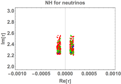
Figure 1: The scatter plots for the real $\tau$ and imaginary $\tau$ in NH. In the $\Delta\chi^{2}$ analysis, the blue color represents the region within 2, green 2-3, and, red 3-5 of $\sqrt{\Delta\chi^{2}}$.

II.4.1 NH

Figure 1 shows the allowed region of $\tau$ within the fundamental region. It suggests that imaginary part of $\tau$ is localized at nearby [$2.2i$–$2.6i$], while whole the region is allowed for real part of $\tau$, where the blue color represents the region within 2, green 2-3, and, red 3-5 of $\sqrt{\Delta\chi^{2}}$. We notice here that real part of $\tau$ tends to be zero, if we focus on the smaller $\Delta\chi^{2}$. It is important since $\tau\sim$ [$2.2i$–$2.6i$], is equivalent the region at nearby one of the fixed point $\tau=i\times\infty$ Okada:2020ukr .

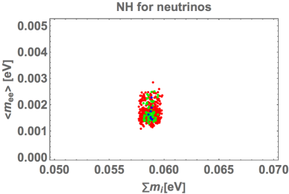
Figure 2: The scatter plots for the neutrinoless double beta decay in terms of sum of neutrino masses. The legend of color is the same as Fig.1.

Figure 2 shows correlation between $\langle m_{ee}\rangle$ and $\sum m_{i}$, where the legend of color is the same as Fig.1. It implies that $\sum m_{i}$ is allowed at the range of [0.058-0.06] eV, and $\langle m_{ee}\rangle$ [0.001-0.0025] eV, which is in favor of our theoretical estimation.

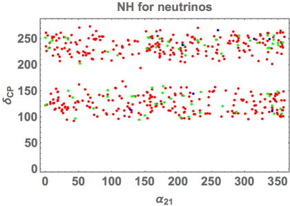
Figure 3: The scatter plots for the Dirac CP phase in terms of Majorana phase. The legend of color is the same as Fig.1.

Figure 3 shows correlation between $\delta_{CP}$ and $\alpha_{21}$, where the legend of color is the same as Fig.1. It reads that Majorana phase tends to be localized at the range of [90-160, 200-270] deg, and whole the range is allowed for the Dirac CP phase.

II.4.2 IH

Since IH needs severe fine-tuning to satisfy the neutrino oscillation data, we show a benchmark point instead of demonstrating figures of NH.

II.4.3 Benchmark point for NH(IH) and consideration the result

We also show a benchmark point for NH and IH in Table 3, where we take $\sqrt{\Delta\chi^{2}}$ is minimum. This table suggests that the allowed region of $\tau$ is in favor of the point at nearby $2.3i$ for both the cases. Here, we study the reason why this region is favored. In this case, one can approximate $[y_{1},y_{2},y_{3}]^{T}\sim[1,0,0]^{T}$ Okada:2020ukr . Under this limit, we find the mass eigenvalues and vectors for the charged-lepton mass matrix to be $(a_{\ell},b_{\ell},c_{\ell})$ and $V_{e_{L}}=1_{3\times 3}$ respectively, and parameters $a_{\ell},b_{\ell}$ can be rewritten in terms of the charged-lepton masses and $c_{\ell}$ as follows:

$$a_{\ell}=\frac{m_{e}}{m_{\tau}}c_{\ell},\quad b_{\ell}=\frac{m_{\mu}}{m_{\tau}}c_{\ell}.$$ (II.24)

Inserting the above relations, our neutrino mass matrix simplifies as follows :

$$\tilde{m}_{\nu}\sim\begin{pmatrix}2\frac{m_{\mu}}{m_{\tau}}\epsilon\epsilon^{\prime}&\frac{m_{\mu}}{m_{\tau}}\epsilon^{\prime}&-\frac{m_{\mu}}{m_{\tau}}\epsilon\\ \frac{m_{\mu}}{m_{\tau}}\epsilon^{\prime}&\frac{m_{e}^{2}}{m_{\tau}^{2}}\epsilon^{\prime 2}&-\frac{m_{\mu}}{m_{\tau}}+\frac{m_{e}^{2}}{m_{\tau}^{2}}\epsilon\epsilon^{\prime}\\ -\frac{m_{\mu}}{m_{\tau}}\epsilon&-\frac{m_{\mu}}{m_{\tau}}+\frac{m_{e}^{2}}{m_{\tau}^{2}}\epsilon\epsilon^{\prime}&\frac{m_{e}^{2}}{m_{\tau}^{2}}\epsilon^{2}\\ \end{pmatrix}.$$ (II.25)

Therefore, we find that

$$\frac{(\tilde{m}_{\nu})_{1,2}}{(\tilde{m}_{\nu})_{1,3}}\sim-\frac{\epsilon^{\prime}}{\epsilon}.$$ (II.26)

Substituting the experimental values at 1$\sigma$ into the above equations with the help of Eq. (III.1) for NH and Eq. (III.2) for IH, we find

$$(NH):\left|\frac{\epsilon^{\prime}}{\epsilon}\right|={\cal O}(0.1-1),\quad(IH):\left|\frac{\epsilon^{\prime}}{\epsilon}\right|={\cal O}(1-10),$$ (II.27)

On the other hand, the experimental result for neutrino mass matrix is given by $\tilde{m}_{\nu}^{exp}\equiv U_{PMNS}\tilde{D}_{\nu}U_{PMNS}^{T}$ as discussed in Sect. II.3 as follows:

$$({\rm NH}):\quad\tilde{m}_{\nu}^{exp}\sim\begin{pmatrix}0&s_{13}s_{23}e^{i\delta_{CP}}&s_{13}c_{23}e^{i\delta_{CP}}\\ s_{13}s_{23}e^{i\delta_{CP}}&s_{23}^{2}&c_{23}s_{23}\\ s_{13}c_{23}e^{i\delta_{CP}}&c_{23}s_{23}&c_{23}^{2}\\ \end{pmatrix},$$ (II.28)

$$({\rm IH}):\quad\tilde{m}_{\nu}^{exp}\sim\begin{pmatrix}c_{12}^{2}+s_{12}^{2}e^{-i\alpha_{21}}&s_{12}c_{12}c_{23}(-1+e^{-i\alpha_{21}})&c_{12}s_{12}s_{23}(1-e^{-i\alpha_{21}})\\ s_{12}c_{12}c_{23}(-1+e^{-i\alpha_{21}})&*&*\\ c_{12}s_{12}s_{23}(1-e^{-i\alpha_{21}})&*&*\\ \end{pmatrix},$$ (II.29)

where we have approximated them substituting $\tilde{m}_{2}<<\tilde{m}_{3}$ for NH and $\tilde{m}_{1}\sim\tilde{m}_{2}$ for IH. $*$’s in IH are abbreviated due to complicated forms because they are not important. Thus, we find

$$({\rm NH}):\quad\frac{(\tilde{m}_{\nu}^{exp})_{1,2}}{(\tilde{m}_{\nu}^{exp})_{1,3}}\sim\frac{s_{23}}{c_{23}},$$ (II.30)

$$({\rm IH}):\quad\frac{(\tilde{m}_{\nu}^{exp})_{1,2}}{(\tilde{m}_{\nu}^{exp})_{1,3}}\sim-\frac{s_{23}}{c_{23}}.$$ (II.31)

Inserting the experimental value for $s_{23}$, one finds

$$\frac{s_{23}}{c_{23}}\sim{\cal O}(1).$$ (II.32)

From Eq. (II.27) and Eq. (II.32), one finds that theoretical estimation would overlap with the experimental result. Hence, we could conclude that allowed region at nearby $\tau=i\times\infty$ is favored for both the cases.

	NH	IH
$\tau$	$-0.000169+2.37i$	$-0.000118+4.30i$
$\frac{\mu^{\prime 2}}{\rm GeV^{2}}$	$1.51\times 10^{-11}$	$1.66\times 10^{-12}$
$[\epsilon,\epsilon^{\prime}]$	$[-0.0432-0.0432i,0.248-0.0631i]$	$[-4.35-0.396i,4.85-0.0573i]$
$[a_{\ell},\ b_{\ell},\ c_{\ell}]$	$[3.72\times 10^{-6},\ 0.00595,\ 0.000706]$	$[2.79\times 10^{-6},\ 0.000586,\ 0.0100]$
$d_{\ell}$	$65.8-117i$	$-42.8-4.36i$
$\Delta m^{2}_{\rm atm}$	$2.52\times 10^{-3}{\rm eV}^{2}$	$2.50\times 10^{-3}{\rm eV}^{2}$
$\Delta m^{2}_{\rm sol}$	$7.30\times 10^{-5}{\rm eV}^{2}$	$7.43\times 10^{-5}{\rm eV}^{2}$
$\sin\theta_{12}$	$0.556$	$0.583$
$\sin\theta_{23}$	$0.685$	$0.666$
$\sin\theta_{13}$	$0.148$	$0.151$
$[\delta_{CP}^{\ell},\ \alpha_{21}]$	$[238^{\circ},\,207^{\circ}]$	$[178^{\circ},\,179^{\circ}]$
$\sum m_{i}$	$58.8$ meV	$99.3$ meV
$\langle m_{ee}\rangle$	$1.48$ meV	$15.2$ meV
$\sqrt{\Delta\chi^{2}}$	$1.48$	$4.99$

Table 3: Numerical benchmark point of our input parameters and observables in NH and IH, where it is taken such that $\sqrt{\Delta\chi^{2}}$ be minimum.

III Conclusions and discussions

We have studied Zee-Babu model with a modular $A_{4}$ symmetry, and searched for predictions under a minimum framework of the charge assignments. We have found that $\tau\sim i\times\infty$ is favored to satisfy the neutrino oscillation data for both of the cases for NH and IH. This is theoretically explainable because it leads to simplified Yukawa couplings $[y_{1}y_{2},y_{3}]^{T}=[1,0,0]^{T}$. Also, we have a specific patterns for phases for NH and IH. The sum of neutrino masses and neutrinoless double beta decay are determined by two experiments of mass squared differences that is direct consequence for Zee-Babu model, which gives rank two neutrino mass matrix. Here, we have also searched for several non-minimum assignments of modular weight that satisfy the neutrino oscillation data, and have found several models as can be seen in Table 4, where the other assignments are the same as the minimum one. Interestingly, all the models favor the fixed point at near by $\tau=i\times\infty$, even though the other predictions are different each other.

	Leptons		Bosons
	$[\bar{L}_{L_{e}},\bar{L}_{L_{\mu}},\bar{L}_{L_{\tau}}]$	$\ell_{R}$	$H$	$s^{-}$	$k^{++}$
$-k_{I}$	$[-2,-6,-6]$	$0$	$0$	$-4$	$0$
$-k_{I}$	$[-2,-2,-4]$	$-2$	$0$	$-4$	$0$
$-k_{I}$	$[-3,-3,-5]$	$-1$	$0$	$-4$	$0$

Table 4: The other models that satisfy the neutrino oscillation data.

Since modular symmetries are frequently discussed in a supersymmetric theory, we mention the supersymmetric extension of the Zee-Babu model. In fact, Zee-Babu model can be extended to a supersymmetric theory, introducing three more chiral super fields with opposite $U(1)_{Y}$ charge of $s^{-},k^{++},H$ Aoki:2010ib . In this case, there are two more diagrams contributing to the neutrino mass matrix at two-loop level from supersymmetric fields. Supposing supersymmetric breaking scale to be much higher than the electroweak scale, we expect supersymmetric contributions are neglected. Thus, we work on the model in a non-supersymmetric theory.

Before closing our paper, it would be worthwhile discussing the other phenomenologies. Typically, Zee-Babu model requires several constraints via lepton universality, lepton flavor violations, and collider physics such as Large Hadron Collider(LHC). As a result, Yukawa couplings $f$ and $g$, and masses of $s^{\pm}$ and $k^{\pm\pm}$ receive constraints. Detail analyses have already been done by several authors Babu:2002uu ; AristizabalSierra:2006gb ; Schmidt:2014zoa ; Nebot:2007bc . In our analysis, however, we do not need to consider these constraints , since whole the constraints are involved in $\mu^{\prime}$ that has free parameters. Thus, we can control this value whatever we want.

Appendix A

Here, using an interesting relation $f(1,-\epsilon,\epsilon^{\prime})^{T}=0$, one straightforwardly finds

$$m_{\nu}(1,-\epsilon,\epsilon^{\prime})^{T}=0.$$

Supposing $V_{e_{L}}=1$, the neutrino mass matrix $m_{\nu}=U_{PMNS}[m_{1},m_{2},m_{3}]U_{PMNS}^{T}$ is written by

$$\begin{split}(m_{\nu})_{\text{ee}}&=m_{1}c_{12}^{2}c_{13}^{2}+m_{2}c_{13}^{2}s_{12}^{2}+m_{3}s_{13}^{2}e^{2i\delta_{CP}},\\ (m_{\nu})_{\text{e$\mu$}}&=m_{2}c_{13}s_{12}(c_{12}c_{23}-s_{12}s_{13}s_{23}e^{-i\delta_{CP}})-m_{1}c_{12}c_{13}(c_{23}s_{12}+c_{12}s_{13}s_{23}e^{-i\delta_{CP}})+m_{3}c_{13}s_{13}s_{23}e^{i\delta_{CP}},\\ (m_{\nu})_{\text{e$\tau$}}&=m_{1}c_{12}c_{13}(s_{12}s_{23}-c_{12}c_{23}s_{13}e^{-i\delta_{CP}})-m_{2}c_{13}s_{12}(c_{12}s_{23}+c_{23}s_{12}s_{13}e^{-i\delta_{CP}})+m_{3}c_{13}s_{13}c_{23}e^{i\delta_{CP}},\\ (m_{\nu})_{\mu\mu}&=m_{1}(c_{23}s_{12}+c_{12}s_{13}s_{23}e^{-i\delta_{CP}})^{2}+m_{2}(c_{12}c_{23}-s_{12}s_{13}s_{23}e^{-i\delta_{CP}})^{2}+m_{3}c_{13}^{2}s_{23}^{2},\\ (m_{\nu})_{\mu\tau}&=-m_{1}(s_{12}s_{23}-c_{12}c_{23}s_{13}e^{-i\delta_{CP}})(c_{23}s_{12}+c_{12}s_{13}s_{23}e^{-i\delta_{CP}})\\ &-m_{2}(c_{12}s_{23}+c_{23}s_{12}s_{13}e^{-i\delta_{CP}})(c_{12}c_{23}-s_{12}s_{13}s_{23}e^{-i\delta_{CP}})+m_{3}c_{13}^{2}c_{23}s_{23},\\ (m_{\nu})_{\tau\tau}&=m_{1}(s_{12}s_{23}-c_{12}c_{23}s_{13}e^{-i\delta_{CP}})^{2}+m_{2}(c_{12}s_{23}+c_{23}s_{12}s_{13}e^{-i\delta_{CP}})^{2}+m_{3}c_{13}^{2}c_{23}^{2}.\end{split}$$

Then, the parameters $\epsilon,\epsilon^{\prime}$ are found to be

$$\begin{split}\epsilon&=\frac{c_{13}\left[s_{13}s_{23}\left(-2m_{1}m_{2}+2m_{3}(c_{12}^{2}m_{2}+m_{1}s_{12}^{2})e^{2i\delta_{CP}}\right)-2c_{12}c_{23}\left(m_{1}-m_{2}\right)m_{3}s_{12}e^{i\delta_{CP}}\right]e^{i\delta_{CP}}}{2m_{1}m_{2}s_{13}^{2}+2c_{13}^{2}m_{3}\left(c_{12}^{2}m_{2}+m_{1}s_{12}^{2}\right)e^{2i\delta_{CP}}},\\ \epsilon^{\prime}&=\frac{c_{13}\left[c_{23}s_{13}\left(m_{1}m_{2}-m_{3}(c_{12}^{2}m_{2}+m_{1}s_{12}^{2})e^{2i\delta_{CP}}\right)-c_{12}\left(m_{1}-m_{2}\right)m_{3}s_{12}s_{23}e^{i\delta_{CP}}\right]e^{i\delta_{CP}}}{m_{1}m_{2}s_{13}^{2}+c_{13}^{2}m_{3}(c_{12}^{2}m_{2}+m_{1}s_{12}^{2})e^{2i\delta_{CP}}}.\\ \end{split}$$

For NH(IH), i.e., $m_{1(3)}=0$, one has

$${({\rm NH})}:$$

$$\epsilon=c_{23}\frac{s_{12}}{c_{12}c_{13}}+s_{23}\frac{s_{13}}{c_{13}}e^{i\delta_{\text{CP}}},\quad\epsilon^{\prime}=s_{23}\frac{s_{12}}{c_{12}c_{13}}-c_{23}\frac{s_{13}}{c_{13}}e^{i\delta_{\text{CP}}},$$ (III.1)

$${({\rm IH})}:$$

$$\epsilon=-s_{23}\frac{c_{13}}{s_{13}}e^{i\delta_{\text{CP}}},\quad\epsilon^{\prime}=c_{23}\frac{c_{13}}{s_{13}}e^{i\delta_{\text{CP}}}.$$ (III.2)

Appendix B

In this appendix, we present several properties of the modular $A_{4}$ symmetry. In general, the modular group $\bar{\Gamma}$ is a group of the linear fractional transformation $\gamma$, acting on the modulus $\tau$ which belongs to the upper-half complex plane and transforms as

$$\tau\longrightarrow\gamma\tau=\frac{a\tau+b}{c\tau+d}\ ,~{}~{}{\rm where}~{}~{}a,b,c,d\in\mathbb{Z}~{}~{}{\rm and}~{}~{}ad-bc=1,~{}~{}{\rm Im}[\tau]>0~{}.$$ (III.3)

This is isomorphic to $PSL(2,\mathbb{Z})=SL(2,\mathbb{Z})/\{I,-I\}$ transformation. Then modular transformation is generated by two transformations $S$ and $T$ defined by:

$$S:\tau\longrightarrow-\frac{1}{\tau}\ ,\qquad\qquad T:\tau\longrightarrow\tau+1\ ,$$ (III.4)

and they satisfy the following algebraic relations,

$$S^{2}=\mathbb{I}\ ,\qquad(ST)^{3}=\mathbb{I}\ .$$ (III.5)

More concretely, we fix the basis of $S$ and $T$ as follows:

$$S=\frac{1}{3}\begin{pmatrix}-1&2&2\\ 2&-1&2\\ 2&2&-1\\ \end{pmatrix},\quad T=\begin{pmatrix}1&0&0\\ 0&\omega&0\\ 0&0&\omega^{2}\\ \end{pmatrix},$$ (III.6)

where $\omega\equiv e^{2\pi i/3}$.

Thus, we introduce the series of groups $\Gamma(N)~{}(N=1,2,3,\dots)$ that is so-called ”principal congruence subgroups of $SL(2,Z)$”, which are defined by

$$\begin{aligned} \Gamma(N)=\left\{\begin{pmatrix}a&b\\ c&d\end{pmatrix}\in SL(2,\mathbb{Z})~{},~{}~{}\begin{pmatrix}a&b\\ c&d\end{pmatrix}=\begin{pmatrix}1&0\\ 0&1\end{pmatrix}~{}~{}({\rm mod}~{}N)\right\}\end{aligned},$$ (III.7)

and we define $\bar{\Gamma}(2)\equiv\Gamma(2)/\{I,-I\}$ for $N=2$. Since the element $-I$ does not belong to $\Gamma(N)$ for $N>2$ case, we have $\bar{\Gamma}(N)=\Gamma(N)$, that are infinite normal subgroup of $\bar{\Gamma}$ known as principal congruence subgroups. We thus obtain finite modular groups as the quotient groups defined by $\Gamma_{N}\equiv\bar{\Gamma}/\bar{\Gamma}(N)$. For these finite groups $\Gamma_{N}$, $T^{N}=\mathbb{I}$ is imposed, and the groups $\Gamma_{N}$ with $N=2,3,4$ and $5$ are isomorphic to $S_{3}$, $A_{4}$, $S_{4}$ and $A_{5}$, respectively deAdelhartToorop:2011re .

Modular forms of level $N$ are holomorphic functions $f(\tau)$ which are transformed under the action of $\Gamma(N)$ given by

$$f(\gamma\tau)=(c\tau+d)^{k}f(\tau)~{},~{}~{}\gamma\in\Gamma(N)~{},$$ (III.8)

where $k$ is the so-called as the modular weight.

Under the modular transformation in Eq.(III.3) in case of $A_{4}$ ($N=3$) modular group, a field $\phi^{(I)}$ is also transformed as

$$\phi^{(I)}\to(c\tau+d)^{-k_{I}}\rho^{(I)}(\gamma)\phi^{(I)},$$ (III.9)

where $-k_{I}$ is the modular weight and $\rho^{(I)}(\gamma)$ denotes a unitary representation matrix of $\gamma\in\Gamma(3)$ ($A_{4}$ representation). Thus Lagrangian such as Yukawa terms can be invariant if sum of modular weight from fields and modular form in corresponding term is zero (also invariant under $A_{4}$ and gauge symmetry).

The kinetic terms and quadratic terms of scalar fields can be written by

$$\frac{|\partial_{\mu}\phi^{(I)}|^{2}}{(-i\tau+i\bar{\tau})^{k_{I}}}~{},\quad\frac{|\phi^{(I)}|^{2}}{(-i\tau+i\bar{\tau})^{k_{I}}}~{},$$ (III.10)

which is invariant under the modular transformation and overall factor is eventually absorbed by a field redefinition consistently. Therefore the Lagrangian associated with these terms should be invariant under the modular symmetry.

The basis of modular forms with weight 2, $Y^{(2)}_{3}=(y_{1},y_{2},y_{3})$, transforming as a triplet of $A_{4}$ is written in terms of Dedekind eta-function $\eta(\tau)$ and its derivative Feruglio:2017spp :

$$y_{1}(\tau) =\frac{i}{2\pi}\left(\frac{\eta^{\prime}(\tau/3)}{\eta(\tau/3)}+\frac{\eta^{\prime}((\tau+1)/3)}{\eta((\tau+1)/3)}+\frac{\eta^{\prime}((\tau+2)/3)}{\eta((\tau+2)/3)}-\frac{27\eta^{\prime}(3\tau)}{\eta(3\tau)}\right)$$

$$\simeq 1+12q+36q^{2}+12q^{3}+\cdots,$$ (III.11)

$$y_{2}(\tau) =\frac{-i}{\pi}\left(\frac{\eta^{\prime}(\tau/3)}{\eta(\tau/3)}+\omega^{2}\frac{\eta^{\prime}((\tau+1)/3)}{\eta((\tau+1)/3)}+\omega\frac{\eta^{\prime}((\tau+2)/3)}{\eta((\tau+2)/3)}\right),$$

$$\simeq-6q^{1/3}(1+7q+8q^{2}+\cdots),$$ (III.12)

$$y_{3}(\tau) =\frac{-i}{\pi}\left(\frac{\eta^{\prime}(\tau/3)}{\eta(\tau/3)}+\omega\frac{\eta^{\prime}((\tau+1)/3)}{\eta((\tau+1)/3)}+\omega^{2}\frac{\eta^{\prime}((\tau+2)/3)}{\eta((\tau+2)/3)}\right)$$

$$\simeq-18q^{2/3}(1+2q+5q^{2}+\cdots),$$ (III.13)

where $q=e^{2\pi i\tau}$, and expansion form in terms of $q$ would sometimes be useful to have numerical analysis.

Then, we can construct the higher order of couplings under $A_{4}$ singlets $Y^{(4)}_{3},\ Y^{(6)}_{3},\ Y^{{}^{\prime}(6)}_{3}$, $Y^{(10)}_{1^{\prime}}$, $Y^{(12)}_{1^{\prime\prime}}$, $Y^{(14)}_{1}$:

$$Y^{(4)}_{1}=y^{2}_{1}+2y_{2}y_{3},\ Y^{(4)}_{1^{\prime}}=y^{2}_{3}+2y_{1}y_{2},\ Y^{(6)}_{1}=y^{3}_{1}+y^{3}_{2}+y^{3}_{3}-3y_{1}y_{2}y_{3},$$ (III.14)

$$Y^{(8)}_{1}=(y_{1}^{2}+2y_{2}y_{3})^{2},\ Y^{(8)}_{1^{\prime}}=(y_{1}^{2}+2y_{2}y_{3})(y_{3}^{2}+2y_{1}y_{2}),\ Y^{(8)}_{1^{\prime\prime}}=(y_{3}^{2}+2y_{1}y_{2})^{2},$$ (III.15)

$$Y^{(10)}_{1^{\prime}}=Y^{(4)}_{1^{\prime}}Y^{(6)}_{1},\ Y^{(12)}_{1^{\prime\prime}}=Y^{(4)}_{1}Y^{(8)}_{1^{\prime\prime}},\ Y^{(14)}_{1^{\prime\prime}}=Y^{(6)}_{1}Y^{(8)}_{1},\$$ (III.16)

$$Y^{(4)}_{3} =(y^{2}_{1}-y_{2}y_{3},y^{2}_{3}-y_{1}y_{2},y^{2}_{2}-y_{1}y_{3}),$$ (III.17)

$$Y^{(6)}_{3} =(y^{3}_{1}+2y_{1}y_{2}y_{3},y_{1}^{2}y_{2}+2y^{2}_{2}y_{3},y^{2}_{1}y_{3}+2y^{2}_{3}y_{2}),$$ (III.18)

$$Y^{(6)}_{3^{\prime}} =(y^{3}_{3}+2y_{1}y_{2}y_{3},y^{2}_{3}y_{1}+2y^{2}_{1}y_{2},y^{2}_{3}y_{2}+2y^{2}_{2}y_{1}),$$ (III.19)

where the above relations are constructed by the multiplication rules under $A_{4}$ as shown below:

$$\begin{pmatrix}a_{1}\\ a_{2}\\ a_{3}\end{pmatrix}_{\bf 3}\otimes\begin{pmatrix}b_{1}\\ b_{2}\\ b_{3}\end{pmatrix}_{\bf 3^{\prime}} =\left(a_{1}b_{1}+a_{2}b_{3}+a_{3}b_{2}\right)_{\bf 1}\oplus\left(a_{3}b_{3}+a_{1}b_{2}+a_{2}b_{1}\right)_{{\bf 1}^{\prime}}$$

$$\oplus\left(a_{2}b_{2}+a_{1}b_{3}+a_{3}b_{1}\right)_{{\bf 1}^{\prime\prime}}$$

$$\oplus\frac{1}{3}\begin{pmatrix}2a_{1}b_{1}-a_{2}b_{3}-a_{3}b_{2}\\ 2a_{3}b_{3}-a_{1}b_{2}-a_{2}b_{1}\\ 2a_{2}b_{2}-a_{1}b_{3}-a_{3}b_{1}\end{pmatrix}_{{\bf 3}}\oplus\frac{1}{2}\begin{pmatrix}a_{2}b_{3}-a_{3}b_{2}\\ a_{1}b_{2}-a_{2}b_{1}\\ a_{3}b_{1}-a_{1}b_{3}\end{pmatrix}_{{\bf 3^{\prime}}\ }\ ,$$

$$a_{1^{\prime}}\otimes\begin{pmatrix}b_{1}\\ b_{2}\\ b_{3}\end{pmatrix}_{\bf 3} =a\begin{pmatrix}b_{3}\\ b_{1}\\ b_{2}\end{pmatrix}_{\bf 3},\quad a_{1^{\prime\prime}}\otimes\begin{pmatrix}b_{1}\\ b_{2}\\ b_{3}\end{pmatrix}_{\bf 3}=a\begin{pmatrix}b_{2}\\ b_{3}\\ b_{1}\end{pmatrix}_{\bf 3},$$

$${\bf 1}\otimes{\bf 1}={\bf 1}\ ,\quad {\bf 1^{\prime}}\otimes{\bf 1^{\prime}}={\bf 1^{\prime\prime}}\ ,\quad{\bf 1^{\prime\prime}}\otimes{\bf 1^{\prime\prime}}={\bf 1^{\prime}}\ ,\quad{\bf 1^{\prime}}\otimes{\bf 1^{\prime\prime}}={\bf 1}\ .$$ (III.20)

References

- (1) A. Zee, Nucl. Phys. B 264, 99 (1986); K. S. Babu, Phys. Lett. B 203, 132 (1988).
- (2) K. S. Babu and C. Macesanu, Phys. Rev. D 67, 073010 (2003) doi:10.1103/PhysRevD.67.073010 [arXiv:hep-ph/0212058 [hep-ph]].
- (3) D. Aristizabal Sierra and M. Hirsch, JHEP 12, 052 (2006) doi:10.1088/1126-6708/2006/12/052 [arXiv:hep-ph/0609307 [hep-ph]].
- (4) D. Schmidt, T. Schwetz and H. Zhang, Nucl. Phys. B 885, 524-541 (2014) doi:10.1016/j.nuclphysb.2014.05.024 [arXiv:1402.2251 [hep-ph]].
- (5) M. Nebot, J. F. Oliver, D. Palao and A. Santamaria, Phys. Rev. D 77, 093013 (2008) doi:10.1103/PhysRevD.77.093013 [arXiv:0711.0483 [hep-ph]].
- (6) F. Feruglio, doi:10.1142/9789813238053_0012 [arXiv:1706.08749 [hep-ph]].
- (7) R. de Adelhart Toorop, F. Feruglio and C. Hagedorn, Nucl. Phys. B 858, 437-467 (2012) doi:10.1016/j.nuclphysb.2012.01.017 [arXiv:1112.1340 [hep-ph]].
- (8) J. C. Criado and F. Feruglio, SciPost Phys. 5, no.5, 042 (2018) doi:10.21468/SciPostPhys.5.5.042 [arXiv:1807.01125 [hep-ph]].
- (9) T. Kobayashi, N. Omoto, Y. Shimizu, K. Takagi, M. Tanimoto and T. H. Tatsuishi, JHEP 11, 196 (2018) doi:10.1007/JHEP11(2018)196 [arXiv:1808.03012 [hep-ph]].
- (10) H. Okada and M. Tanimoto, Phys. Lett. B 791, 54-61 (2019) doi:10.1016/j.physletb.2019.02.028 [arXiv:1812.09677 [hep-ph]].
- (11) T. Nomura and H. Okada, Phys. Lett. B 797, 134799 (2019) doi:10.1016/j.physletb.2019.134799 [arXiv:1904.03937 [hep-ph]].
- (12) H. Okada and M. Tanimoto, Eur. Phys. J. C 81, no.1, 52 (2021) doi:10.1140/epjc/s10052-021-08845-y [arXiv:1905.13421 [hep-ph]].
- (13) F. J. de Anda, S. F. King and E. Perdomo, Phys. Rev. D 101, no.1, 015028 (2020) doi:10.1103/PhysRevD.101.015028 [arXiv:1812.05620 [hep-ph]].
- (14) P. P. Novichkov, S. T. Petcov and M. Tanimoto, Phys. Lett. B 793, 247-258 (2019) doi:10.1016/j.physletb.2019.04.043 [arXiv:1812.11289 [hep-ph]].
- (15) T. Nomura and H. Okada, Nucl. Phys. B 966, 115372 (2021) doi:10.1016/j.nuclphysb.2021.115372 [arXiv:1906.03927 [hep-ph]].
- (16) H. Okada and Y. Orikasa, [arXiv:1907.13520 [hep-ph]].
- (17) G. J. Ding, S. F. King and X. G. Liu, JHEP 09, 074 (2019) doi:10.1007/JHEP09(2019)074 [arXiv:1907.11714 [hep-ph]].
- (18) T. Nomura, H. Okada and O. Popov, Phys. Lett. B 803, 135294 (2020) doi:10.1016/j.physletb.2020.135294 [arXiv:1908.07457 [hep-ph]].
- (19) T. Kobayashi, Y. Shimizu, K. Takagi, M. Tanimoto and T. H. Tatsuishi, Phys. Rev. D 100, no.11, 115045 (2019) [erratum: Phys. Rev. D 101, no.3, 039904 (2020)] doi:10.1103/PhysRevD.100.115045 [arXiv:1909.05139 [hep-ph]].
- (20) T. Asaka, Y. Heo, T. H. Tatsuishi and T. Yoshida, JHEP 01, 144 (2020) doi:10.1007/JHEP01(2020)144 [arXiv:1909.06520 [hep-ph]].
- (21) D. Zhang, Nucl. Phys. B 952, 114935 (2020) doi:10.1016/j.nuclphysb.2020.114935 [arXiv:1910.07869 [hep-ph]].
- (22) G. J. Ding, S. F. King, X. G. Liu and J. N. Lu, JHEP 12, 030 (2019) doi:10.1007/JHEP12(2019)030 [arXiv:1910.03460 [hep-ph]].
- (23) T. Kobayashi, T. Nomura and T. Shimomura, Phys. Rev. D 102, no.3, 035019 (2020) doi:10.1103/PhysRevD.102.035019 [arXiv:1912.00637 [hep-ph]].
- (24) T. Nomura, H. Okada and S. Patra, Nucl. Phys. B 967, 115395 (2021) doi:10.1016/j.nuclphysb.2021.115395 [arXiv:1912.00379 [hep-ph]].
- (25) X. Wang, Nucl. Phys. B 957, 115105 (2020) doi:10.1016/j.nuclphysb.2020.115105 [arXiv:1912.13284 [hep-ph]].
- (26) H. Okada and Y. Shoji, Nucl. Phys. B 961, 115216 (2020) doi:10.1016/j.nuclphysb.2020.115216 [arXiv:2003.13219 [hep-ph]].
- (27) H. Okada and M. Tanimoto, [arXiv:2005.00775 [hep-ph]].
- (28) M. K. Behera, S. Singirala, S. Mishra and R. Mohanta, [arXiv:2009.01806 [hep-ph]].
- (29) M. K. Behera, S. Mishra, S. Singirala and R. Mohanta, [arXiv:2007.00545 [hep-ph]].
- (30) T. Nomura and H. Okada, [arXiv:2007.04801 [hep-ph]].
- (31) T. Nomura and H. Okada, [arXiv:2007.15459 [hep-ph]].
- (32) T. Asaka, Y. Heo and T. Yoshida, Phys. Lett. B 811, 135956 (2020) doi:10.1016/j.physletb.2020.135956 [arXiv:2009.12120 [hep-ph]].
- (33) H. Okada and M. Tanimoto, Phys. Rev. D 103, no.1, 015005 (2021) doi:10.1103/PhysRevD.103.015005 [arXiv:2009.14242 [hep-ph]].
- (34) K. I. Nagao and H. Okada, [arXiv:2010.03348 [hep-ph]].
- (35) H. Okada and M. Tanimoto, JHEP 03, 010 (2021) doi:10.1007/JHEP03(2021)010 [arXiv:2012.01688 [hep-ph]].
- (36) C. Y. Yao, J. N. Lu and G. J. Ding, JHEP 05 (2021), 102 doi:10.1007/JHEP05(2021)102 [arXiv:2012.13390 [hep-ph]].
- (37) P. Chen, G. J. Ding and S. F. King, JHEP 04 (2021), 239 doi:10.1007/JHEP04(2021)239 [arXiv:2101.12724 [hep-ph]].
- (38) M. Kashav and S. Verma, [arXiv:2103.07207 [hep-ph]].
- (39) H. Okada, Y. Shimizu, M. Tanimoto and T. Yoshida, [arXiv:2105.14292 [hep-ph]].
- (40) I. de Medeiros Varzielas and J. Lourenço, [arXiv:2107.04042 [hep-ph]].
- (41) T. Nomura, H. Okada and Y. Orikasa, [arXiv:2106.12375 [hep-ph]].
- (42) P. T. P. Hutauruk, D. W. Kang, J. Kim and H. Okada, [arXiv:2012.11156 [hep-ph]].
- (43) G. J. Ding, S. F. King and J. N. Lu, [arXiv:2108.09655 [hep-ph]].
- (44) K. I. Nagao and H. Okada, [arXiv:2108.09984 [hep-ph]].
- (45) Georgianna Charalampous, Stephen F. King, George K. Leontaris, Ye-Ling Zhou [arXiv:2109.11379 [hep-ph]].
- (46) T. Kobayashi, K. Tanaka and T. H. Tatsuishi, Phys. Rev. D 98, no.1, 016004 (2018) doi:10.1103/PhysRevD.98.016004 [arXiv:1803.10391 [hep-ph]].
- (47) T. Kobayashi, Y. Shimizu, K. Takagi, M. Tanimoto, T. H. Tatsuishi and H. Uchida, Phys. Lett. B 794, 114-121 (2019) doi:10.1016/j.physletb.2019.05.034 [arXiv:1812.11072 [hep-ph]].
- (48) T. Kobayashi, Y. Shimizu, K. Takagi, M. Tanimoto and T. H. Tatsuishi, PTEP 2020, no.5, 053B05 (2020) doi:10.1093/ptep/ptaa055 [arXiv:1906.10341 [hep-ph]].
- (49) H. Okada and Y. Orikasa, Phys. Rev. D 100, no.11, 115037 (2019) doi:10.1103/PhysRevD.100.115037 [arXiv:1907.04716 [hep-ph]].
- (50) S. Mishra, [arXiv:2008.02095 [hep-ph]].
- (51) X. Du and F. Wang, JHEP 02, 221 (2021) doi:10.1007/JHEP02(2021)221 [arXiv:2012.01397 [hep-ph]].
- (52) J. T. Penedo and S. T. Petcov, Nucl. Phys. B 939, 292-307 (2019) doi:10.1016/j.nuclphysb.2018.12.016 [arXiv:1806.11040 [hep-ph]].
- (53) P. P. Novichkov, J. T. Penedo, S. T. Petcov and A. V. Titov, JHEP 04, 005 (2019) doi:10.1007/JHEP04(2019)005 [arXiv:1811.04933 [hep-ph]].
- (54) T. Kobayashi, Y. Shimizu, K. Takagi, M. Tanimoto and T. H. Tatsuishi, JHEP 02, 097 (2020) doi:10.1007/JHEP02(2020)097 [arXiv:1907.09141 [hep-ph]].
- (55) S. F. King and Y. L. Zhou, Phys. Rev. D 101, no.1, 015001 (2020) doi:10.1103/PhysRevD.101.015001 [arXiv:1908.02770 [hep-ph]].
- (56) H. Okada and Y. Orikasa, [arXiv:1908.08409 [hep-ph]].
- (57) J. C. Criado, F. Feruglio and S. J. D. King, JHEP 02, 001 (2020) doi:10.1007/JHEP02(2020)001 [arXiv:1908.11867 [hep-ph]].
- (58) X. Wang and S. Zhou, JHEP 05, 017 (2020) doi:10.1007/JHEP05(2020)017 [arXiv:1910.09473 [hep-ph]].
- (59) Y. Zhao and H. H. Zhang, JHEP 03 (2021), 002 doi:10.1007/JHEP03(2021)002 [arXiv:2101.02266 [hep-ph]].
- (60) S. F. King and Y. L. Zhou, JHEP 04 (2021), 291 doi:10.1007/JHEP04(2021)291 [arXiv:2103.02633 [hep-ph]].
- (61) G. J. Ding, S. F. King and C. Y. Yao, [arXiv:2103.16311 [hep-ph]].
- (62) X. Zhang and S. Zhou, [arXiv:2106.03433 [hep-ph]].
- (63) Bu-Yao Qu, Xiang-Gan Liu, Ping-Tao Chen, Gui-Jun Ding [arXiv:2106.11659 [hep-ph]].
- (64) T. Nomura and H. Okada, [arXiv:2109.04157 [hep-ph]].
- (65) P. P. Novichkov, J. T. Penedo, S. T. Petcov and A. V. Titov, JHEP 04, 174 (2019) doi:10.1007/JHEP04(2019)174 [arXiv:1812.02158 [hep-ph]].
- (66) G. J. Ding, S. F. King and X. G. Liu, Phys. Rev. D 100, no.11, 115005 (2019) doi:10.1103/PhysRevD.100.115005 [arXiv:1903.12588 [hep-ph]].
- (67) X. Wang, B. Yu and S. Zhou, Phys. Rev. D 103, no.7, 076005 (2021) doi:10.1103/PhysRevD.103.076005 [arXiv:2010.10159 [hep-ph]].
- (68) C. Y. Yao, X. G. Liu and G. J. Ding, Phys. Rev. D 103, no.9, 095013 (2021) doi:10.1103/PhysRevD.103.095013 [arXiv:2011.03501 [hep-ph]].
- (69) X. Wang and S. Zhou, [arXiv:2102.04358 [hep-ph]].
- (70) M. K. Behera and R. Mohanta, [arXiv:2108.01059 [hep-ph]].
- (71) A. Baur, H. P. Nilles, A. Trautner and P. K. S. Vaudrevange, Phys. Lett. B 795, 7-14 (2019) doi:10.1016/j.physletb.2019.03.066 [arXiv:1901.03251 [hep-th]].
- (72) I. de Medeiros Varzielas, S. F. King and Y. L. Zhou, Phys. Rev. D 101, no.5, 055033 (2020) doi:10.1103/PhysRevD.101.055033 [arXiv:1906.02208 [hep-ph]].
- (73) X. G. Liu and G. J. Ding, JHEP 08, 134 (2019) doi:10.1007/JHEP08(2019)134 [arXiv:1907.01488 [hep-ph]].
- (74) P. Chen, G. J. Ding, J. N. Lu and J. W. F. Valle, Phys. Rev. D 102, no.9, 095014 (2020) doi:10.1103/PhysRevD.102.095014 [arXiv:2003.02734 [hep-ph]].
- (75) C. C. Li, X. G. Liu and G. J. Ding, [arXiv:2108.02181 [hep-ph]].
- (76) P. P. Novichkov, J. T. Penedo and S. T. Petcov, Nucl. Phys. B 963, 115301 (2021) doi:10.1016/j.nuclphysb.2020.115301 [arXiv:2006.03058 [hep-ph]].
- (77) X. G. Liu, C. Y. Yao and G. J. Ding, Phys. Rev. D 103, no.5, 056013 (2021) doi:10.1103/PhysRevD.103.056013 [arXiv:2006.10722 [hep-ph]].
- (78) S. Kikuchi, T. Kobayashi, H. Otsuka, S. Takada and H. Uchida, JHEP 11, 101 (2020) doi:10.1007/JHEP11(2020)101 [arXiv:2007.06188 [hep-th]].
- (79) Y. Almumin, M. C. Chen, V. Knapp-Pérez, S. Ramos-Sánchez, M. Ratz and S. Shukla, JHEP 05 (2021), 078 doi:10.1007/JHEP05(2021)078 [arXiv:2102.11286 [hep-th]].
- (80) G. J. Ding, F. Feruglio and X. G. Liu, SciPost Phys. 10 (2021), 133 doi:10.21468/SciPostPhys.10.6.133 [arXiv:2102.06716 [hep-ph]].
- (81) F. Feruglio, V. Gherardi, A. Romanino and A. Titov, JHEP 05 (2021), 242 doi:10.1007/JHEP05(2021)242 [arXiv:2101.08718 [hep-ph]].
- (82) S. Kikuchi, T. Kobayashi and H. Uchida, [arXiv:2101.00826 [hep-th]].
- (83) P. P. Novichkov, J. T. Penedo and S. T. Petcov, JHEP 04 (2021), 206 doi:10.1007/JHEP04(2021)206 [arXiv:2102.07488 [hep-ph]].
- (84) G. Altarelli and F. Feruglio, Rev. Mod. Phys. 82, 2701-2729 (2010) doi:10.1103/RevModPhys.82.2701 [arXiv:1002.0211 [hep-ph]].
- (85) H. Ishimori, T. Kobayashi, H. Ohki, Y. Shimizu, H. Okada and M. Tanimoto, Prog. Theor. Phys. Suppl. 183, 1-163 (2010) doi:10.1143/PTPS.183.1 [arXiv:1003.3552 [hep-th]].
- (86) H. Ishimori, T. Kobayashi, H. Ohki, H. Okada, Y. Shimizu and M. Tanimoto, Lect. Notes Phys. 858, 1-227 (2012) doi:10.1007/978-3-642-30805-5
- (87) D. Hernandez and A. Y. Smirnov, Phys. Rev. D 86, 053014 (2012) doi:10.1103/PhysRevD.86.053014 [arXiv:1204.0445 [hep-ph]].
- (88) S. F. King and C. Luhn, Rept. Prog. Phys. 76, 056201 (2013) doi:10.1088/0034-4885/76/5/056201 [arXiv:1301.1340 [hep-ph]].
- (89) S. F. King, A. Merle, S. Morisi, Y. Shimizu and M. Tanimoto, New J. Phys. 16, 045018 (2014) doi:10.1088/1367-2630/16/4/045018 [arXiv:1402.4271 [hep-ph]].
- (90) S. F. King, Prog. Part. Nucl. Phys. 94, 217-256 (2017) doi:10.1016/j.ppnp.2017.01.003 [arXiv:1701.04413 [hep-ph]].
- (91) S. T. Petcov, Eur. Phys. J. C 78, no.9, 709 (2018) doi:10.1140/epjc/s10052-018-6158-5 [arXiv:1711.10806 [hep-ph]].
- (92) A. Baur, H. P. Nilles, A. Trautner and P. K. S. Vaudrevange, Nucl. Phys. B 947, 114737 (2019) doi:10.1016/j.nuclphysb.2019.114737 [arXiv:1908.00805 [hep-th]].
- (93) T. Kobayashi, Y. Shimizu, K. Takagi, M. Tanimoto, T. H. Tatsuishi and H. Uchida, Phys. Rev. D 101, no.5, 055046 (2020) doi:10.1103/PhysRevD.101.055046 [arXiv:1910.11553 [hep-ph]].
- (94) P. P. Novichkov, J. T. Penedo, S. T. Petcov and A. V. Titov, JHEP 07, 165 (2019) doi:10.1007/JHEP07(2019)165 [arXiv:1905.11970 [hep-ph]].
- (95) M. Tanimoto and K. Yamamoto, [arXiv:2106.10919 [hep-ph]].
- (96) M. C. Chen, S. Ramos-Sánchez and M. Ratz, Phys. Lett. B 801, 135153 (2020) doi:10.1016/j.physletb.2019.135153 [arXiv:1909.06910 [hep-ph]].
- (97) I. de Medeiros Varzielas, M. Levy and Y. L. Zhou, JHEP 11, 085 (2020) doi:10.1007/JHEP11(2020)085 [arXiv:2008.05329 [hep-ph]].
- (98) [ATLAS Collaboration], Report No. ATLAS-CONF-2013-049.
- (99) Z. Maki, M. Nakagawa and S. Sakata, Prog. Theor. Phys. 28, 870-880 (1962) doi:10.1143/PTP.28.870
- (100) A. Gando et al. [KamLAND-Zen], Phys. Rev. Lett. 117, no.8, 082503 (2016) doi:10.1103/PhysRevLett.117.082503 [arXiv:1605.02889 [hep-ex]].
- (101) I. Esteban, M. C. Gonzalez-Garcia, A. Hernandez-Cabezudo, M. Maltoni and T. Schwetz, JHEP 01, 106 (2019) doi:10.1007/JHEP01(2019)106 [arXiv:1811.05487 [hep-ph]].
- (102) PDG
- (103) K. m. Cheung, Phys. Lett. B 517, 167 (2001) doi:10.1016/S0370-2693(01)00973-X [hep-ph/0106251].
- (104) See for example, M. Aaboud et al. [ATLAS Collaboration], New J. Phys. 18, no. 9, 093016 (2016) doi:10.1088/1367-2630/18/9/093016 [arXiv:1605.06035 [hep-ex]].
- (105) M. Aoki, S. Kanemura, T. Shindou and K. Yagyu, JHEP 07, 084 (2010) [erratum: JHEP 11, 049 (2010)] doi:10.1007/JHEP07(2010)084 [arXiv:1005.5159 [hep-ph]]. Copy to ClipboardDownload