Spin oscillations of a single-mode polariton system driven by a plane wave

Abstract

Theoretical study is performed of a single-mode polariton system with linear coupling of spin components. When combined with an ordinary two-particle interaction, the spin coupling involves a spontaneous symmetry breaking accompanied by a switch from linear to circular polarization under resonant driving. The asymmetric steady states can also lose stability, giving way to oscillatory and chaotic dynamics. Here, we explore a continuous transformation between the multistable regime, where the system is steady and locked in phase to the pump but has a broken spin symmetry, and full-span oscillations of the circular-polarization degree, owing to which the symmetry is effectively reestablished. Such oscillations are analogous to the intrinsic Josephson effect and prove to be robust against arbitrarily strong perturbations. Transitional phenomena include the Hopf bifurcation, spin bistability of limit cycles, and continuous transitions to and from dynamical chaos through series of period doubling/halving events.

I Introduction

Being coupled exciton-photon pairs, cavity polaritons form coherent states under resonant excitation [1, 2, 3, 4]. As a rule, the energy level of such a driven bosonic condensate matches the frequency of the pump wave, in analogy to a damped oscillator excited by a harmonic force, so that the condensate is locked in phase to the pump. Interaction of polaritons leads to optical multistability which manifests itself in sharp threshold transitions between steady states in response to varying excitation parameters [5, 6, 7, 8, 9, 10, 11, 12, 13, 14, 15, 16, 17]. However, any nontrivial dynamics of a simple condensate driven by a plane wave is naturally hampered. It is of no surprise that certain ways to release the phase locking exist for inhomogeneous, relatively complex polariton systems [18, 19, 20, 21, 22]. On the other hand, it was found that even a single-mode system driven at normal incidence may behave “freely”, which occurs when all of its locked states get unstable [23, 24, 25, 26]. Here, we extensively study the onset of such a global instability, with a focus on a transition from steady states to self-persistent oscillations depending on the excitation parameters.

This study is restricted to a system with a few effective degrees of freedom described by complex-valued amplitudes $\psi_{+}$ and $\psi_{-}$ of two spin components. A similar model was studied in Ref. [27] dealing with a double-well Josephson junction in which two coherent states are coupled by tunneling through a spatial barrier. Such a system was shown to have an oscillatory regime in a particular highly unstable situation when one of two wells is pumped from the outside but, nevertheless, has a much smaller steady-state amplitude compared to the other. Soon afterwards, a different model with two wells was found to display dynamical chaos [28]; it was relatively complex, however, being dependent on both the spatial junction and spin coupling and thus including four rather than two coherent components. A more recent example of oscillations in a continuously pumped polariton system is given by Ref. [29] which considers a small micropillar with a nonlinear coupling of two quantized levels. Finally, a certain combination of resonant and nonresonant excitation sources can result in a pseudoconservative behavior characterized by a fully compensated dissipation of polaritons [30].

The polariton system considered here is comparatively simple but exhibits an extremely wide variety of complex dynamical states, both chaotic and regular. Theoretically speaking, its key feature is the spontaneous breakdown of the spin symmetry, which is possible owing to linear coupling of two spin components [26]. Even if they are fully identical and equally pumped, one of two components is suppressed upon reaching a critical pump amplitude, so that polaritons acquire very high right- or left-handed circular polarization [31, 32, 33]. In turn, oscillations or dynamical chaos occur irrespective of the initial conditions only when all steady-state solutions, symmetric and asymmetric, prove to be unstable for a given pump wave. This leads us to the problem of finding the complete set of such solutions. Earlier, we used to calculate them numerically for some particular combinations of parameters [23], which, obviously, does not allow one to grasp the whole picture. Here, we report general steady-state solutions along with explicit formulae for the spectra of elementary excitations.

In contrast to Refs. [23] and [24] which demonstrated sharp switches from steady states to chaos, this work is devoted to a continuous transition between different, mostly regular, dynamical regimes in the course of varying pump amplitude $f$. Namely, we have found that steady condensate states with broken symmetry may continuously turn into limit cycles. Since there are two spin states feasible under the same external conditions, the corresponding limit cycles are also twinned in phase space. They are completely distinct near the bifurcation point; however, expansion of a given periodic orbit upon varying $f$ makes it approach the twin one, which opens the possibility of switches between two spin domains and leads to their unification. After a pair of alternative orbits have merged, they run through the whole range of circular-polarization degrees from $-1$ to $+1$ and represent a new, purely dynamical symmetric state which is stable against arbitrary perturbations.

In what follows, the base model is introduced in Sec. II. Section III is aimed at finding the complete set of fixed-point solutions, after which we determine the conditions of their bifurcations into nonsteady states. Section IV deals with a variety of periodic and chaotic dynamical states and their continuous transformations. Section V contains a general discussion and concluding remarks.

II Base model

The coherently excited system of cavity polaritons obeys the following wave equations [1],

$$i\hbar\frac{\partial\psi_{\pm}}{\partial t}=\left(E_{0}-i\gamma+V\psi_{\pm}^{*}\psi_{\pm}^{\vphantom{*}}\right)\psi_{\pm}^{\vphantom{*}}+\frac{g}{2}\psi_{\mp}^{\vphantom{*}}+f_{\pm}^{\vphantom{*}}e^{-iE_{p}t/\hbar},$$ (1)

where $\psi_{+}$ and $\psi_{-}$ are complex-valued amplitudes of two spin components, $E_{0}$ and $\gamma$ are the polariton energy and decay rate, $g$ is the spin coupling rate, $V$ is the polariton-polariton interaction constant, $f_{+}$ and $f_{-}$ are the pump amplitudes corresponding to the right- and left-handed polarizations of light, $E_{p}/\hbar$ is the pump frequency that is assumed to be close to the polariton resonance. The pump wave vector is zero, which corresponds to normal incidence of the driving wave.

For a planar two-dimensional system, $\psi_{\pm}$ depend on space and time, whereas $E_{0}=E_{0}(-i\hbar\nabla)$ is an operator determined by the dispersion law of the lower polariton branch. For a zero-dimensional system representing a small micropillar, $E_{0}$ means the ground level of size quantization. On the assumption that all other levels play no role, the equations are projected onto the corresponding spatial eigenstate; as a result, $\psi_{+}$ and $\psi_{-}$ depend only on time. The same equations describe an effectively spinless system with two quantum wells [27]. As shown in Ref. [29], similar equations also hold for a spinless system in a micropillar when one takes into account the interaction of two quantized levels; however, their coupling rate $g$ appears to be amplitude-dependent.

In case if $f_{+}=f_{-}=0$ and $\gamma=0$, model (1) is reduced to a simple Josephson junction. The eigenlevels are split ($E=E_{0}\pm g/2$ for $|\psi_{\pm}|\to 0$), therefore the phase difference of two components varies with time and involves oscillations. Among other bosonic systems ([34, 35, 36]), such phenomenon is displayed by a freely evolving pair of coupled polariton condensates [37, 38, 39]. The spin oscillations in a pointlike system are referred to as the intrinsic Josephson effect [40, 41, 33] owing to exactly the same form of the equations.

Everything is changed if the system is driven directly, i. e., $f_{+}$ or $f_{-}$ is nonzero. In this case Eqs. (1) have solutions of the form $\psi_{\pm}(t)=\bar{\psi}_{\pm}e^{-iE_{p}\hbar/t}$. The Josephson oscillations are no longer possible since both components oscillate at the same “forced” frequency. Time-independent amplitudes $\bar{\psi}_{+}$ and $\bar{\psi}_{-}$ obey a set of algebraic equations

$$\left(D+i\gamma-V|\bar{\psi}_{+}|^{2}\right)\bar{\psi}_{+}-\frac{g}{2}\bar{\psi}_{-} =f_{+},$$ (2)

$$\left(D+i\gamma-V|\bar{\psi}_{-}|^{2}\right)\bar{\psi}_{-}-\frac{g}{2}\bar{\psi}_{+} =f_{-},$$ (3)

where $D=E_{p}-E_{0}$ (pump detuning). Such solutions are usually called steady states, or fixed points, because $E_{p}$ can be taken as zero without loss of generality.

The dissipative character of the system $(\gamma>0)$ is crucially important. Owing to dissipation, all solutions would be guaranteed to have the forced frequency $E_{p}/\hbar$ at $t\to\infty$ if the interaction constant $V$ were zero. At the same time, nonlinearity does not automatically lead to a nonsteady behavior. If $V>0$ but $g=0$, then even a two-dimensional model (1) with many degrees of freedom evolves to a plane-wave state oscillating at $E=E_{p}$; this final state is asymptotically stable, so that all weak perturbations decay with time.

Thus, the fixed-point states are the “most common” attractors of the phase trajectory for $f_{\pm}\neq 0$ and $\gamma>0$ [26]. A different—nonsteady—type of solutions comes into being only when all fixed points become unstable.

III Fixed-point states and their bifurcations

Let us solve Eqs. (2), (3) at $f_{+}=f_{-}=f$. Notice that in this case the model is spin-symmetric. Since the right-hand sides of the two equations are the same, one can equate the left-hand sides and have

$$\frac{\bar{\psi}_{-}}{\bar{\psi}_{+}}=\frac{a+i\gamma-\mu_{+}}{a+i\gamma-\mu_{-}},$$ (4)

where $\bar{\psi}_{+}\neq 0$ and

$$\mu_{\pm}=V|\bar{\psi}_{\pm}|^{2},\quad a=D+\frac{g}{2}.$$ (5)

Taking the absolute square of (4) yields

$$\mu_{+}^{3}-\mu_{-}^{3}-2a(\mu_{+}^{2}-\mu_{-}^{2})+(a^{2}+\gamma^{2})(\mu_{+}-\mu_{-})=0.$$ (6)

When considering the asymmetric states with $\mu_{+}\neq\mu_{-}$, one may cancel $\mu_{+}-\mu_{-}$ from (6), which results in

$$w^{2}-(u-a)^{2}=\gamma^{2},$$ (7)

where

$$u=\mu_{+}+\mu_{-},\quad w=\sqrt{\mu_{+}\mu_{-}}.$$ (8)

Equation (7) suggests that one of two spin components vanishes at $u=a$ and $\gamma\to 0$. In general, not all combinations of $u$ and $w$ are possible in accordance with their definition. Indeed,

$$0<(\mu_{+}-\mu_{-})^{2}=u^{2}-4w^{2}=u^{2}-4\,\bigl{[}(u-a)^{2}+\gamma^{2}\bigr{]}.$$ (9)

The inequality is satisfied for $l_{1}<u<l_{2}$, where

$$l_{1,2}=\frac{2}{3}\Bigl{(}2a\mp\sqrt{a^{2}-3\gamma^{2}}\Bigr{)}.$$ (10)

The “most asymmetric” state with $u\approx a$ is seen to be inside the allowed interval, given that $D$ and $g$ are positive and sufficiently great compared to $\gamma$. This condition is always assumed hereafter.

In order to find $u$ as a function of $f,$ one can start with finding the reverse dependence $f=f(u)$. To do so, we multiply both sides of Eqs. (2) and (3) by their respective complex conjugates and then sum up the two equations. The result depends on $\mu_{\pm}$ and $\bar{\psi}_{+}^{*}\bar{\psi}_{-}^{\vphantom{*}}+\bar{\psi}_{-}^{*}\bar{\psi}_{+}^{\vphantom{*}}$; however, the latter quantity also can be expressed in terms of $\mu_{\pm}$ using (4). Specifically,

$$\bar{\psi}_{+}^{*}\bar{\psi}_{-}^{\vphantom{*}}+\bar{\psi}_{-}^{*}\bar{\psi}_{+}^{\vphantom{*}}=\left[(a-\mu_{+})(a-\mu_{-})+\gamma^{2}\right]\\ {}\times\left[\frac{\mu_{+}}{(a-\mu_{-})^{2}+\gamma^{2}}+\frac{\mu_{-}}{(a-\mu_{+})^{2}+\gamma^{2}}\right].$$ (11)

The symmetry between $\mu_{+}$ and $\mu_{-}$ suggests that all $\mu$ can be rewritten in terms of $u$ and $w^{2}$, after which $w^{2}$ is easily eliminated using (7). In so doing, after a lengthy calculation one arrives at the final expression:

$$|f|^{2}=\frac{1}{V}\left((2a-u)\,(D-u)^{2}+\frac{\gamma^{2}\,(2D-u)^{2}}{2a-u}\right)$$ (12)

for $u\in(l_{1},l_{2})$. The singularity point $u=2a$ is never reached, because $l_{2}<2a$ so long as $\gamma>0$. Eq. (12) can be reduced to a quartic equation for $u$ which is solvable in a general way. However, the main features of the solutions can be understood using the already obtained reverse dependence $f(u)$. Below, without loss of generality we assume $f$ to be real-valued and positive.

Consider a region around $u\sim a$. If $\gamma$ is noticeably smaller than $a$, one can disregard the second term in (12). Therefore, equation $df/du=0$, which determines the turning points of the solutions, becomes quadratic. It has the following roots,

$$u_{1}=2a-(D+g)=D,\quad u_{2}=2a-\frac{D+g}{3},$$ (13)

whereas the corresponding values of $f^{2}$ are

$$f_{1}^{2}=0,\quad f_{2}^{2}=\frac{4}{27\,V}(D+g)^{3}.$$ (14)

The interval from $\max\{u_{1},l_{1}\}$ to $u_{2}$, wherein function $u(f)$ is single-valued and has positive derivative, is the main domain of asymmetric solutions which will be further analyzed in this work.

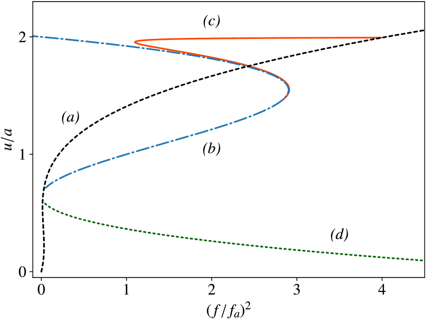
Figure 1: Fixed-point states in case of a spin-symmetric excitation. (a) symmetric states (15) with $\bar{\psi}_{+}=\bar{\psi}_{-}$; (b) approximate asymmetric solution $f^{2}(u)=(2a-u)(D-u)^{2}/V$; (c) exact asymmetric solution (12) in a region where it is noticeably different from (b); (d) spurious branch $(u<l_{1})$. Parameters: $g=9\gamma$, $D=8.1\gamma$; $f_{a}=ag^{2}/4V$.

Figure 1 exemplifies the full set of the fixed-point solutions obtained at $g=9\gamma$ and $D=0.9g$. First, it contains the spin-symmetric branch with $\bar{\psi}_{+}=\bar{\psi}_{-}$ for each $f$ (curve a). The corresponding expression for $f^{2}(u)$ is easily obtained by taking the absolute square of Eq. (2) or (3), which yields

$$f^{2}_{\mathrm{symm}}=\frac{u}{2V}\biggl{[}\left(D-\frac{g}{2}-\frac{u}{2}\right)^{2}+\gamma^{2}\biggr{]}.$$ (15)

This formula reproduces the well-known S-shaped curve of a spinless polariton system [5] with $V|\psi|^{2}=u/2$ and pump detuning $D-g/2$ (the latter quantity equals the difference between $E_{p}$ and the eigenlevel whose polarization matches that of the pump wave).

Also shown in Fig. 1 are the approximate asymmetric solution obtained from (12) by dropping the second term (curve b), the exact solution in the vicinity of $u=2a$ (curve c), and the spurious branch for $u<l_{1}$ (curve d). Branches b and d are seen to combine into an upside-down S-shaped curve. Indeed, if we substitute $u=2a-u^{\prime}$ in (12), then for $\gamma\to 0$ we once again arrive at the usual response function describing a spinless system whose effective $V|\psi|^{2}$ and pump detuning are equal to $u^{\prime}$ and $D^{\prime}=D+g$, respectively, which is also evident from Eqs. (13) and (14). Notice that $D^{\prime}$ is quite large and exceeds even the pump detuning from the farther eigenlevel (i. e., $D+g/2$). Since $f_{2}^{2}-f_{1}^{2}\propto D^{\prime 3}$, function $u(f)$ changes very slowly throughout the main asymmetric domain $(l_{1},u_{2})$.

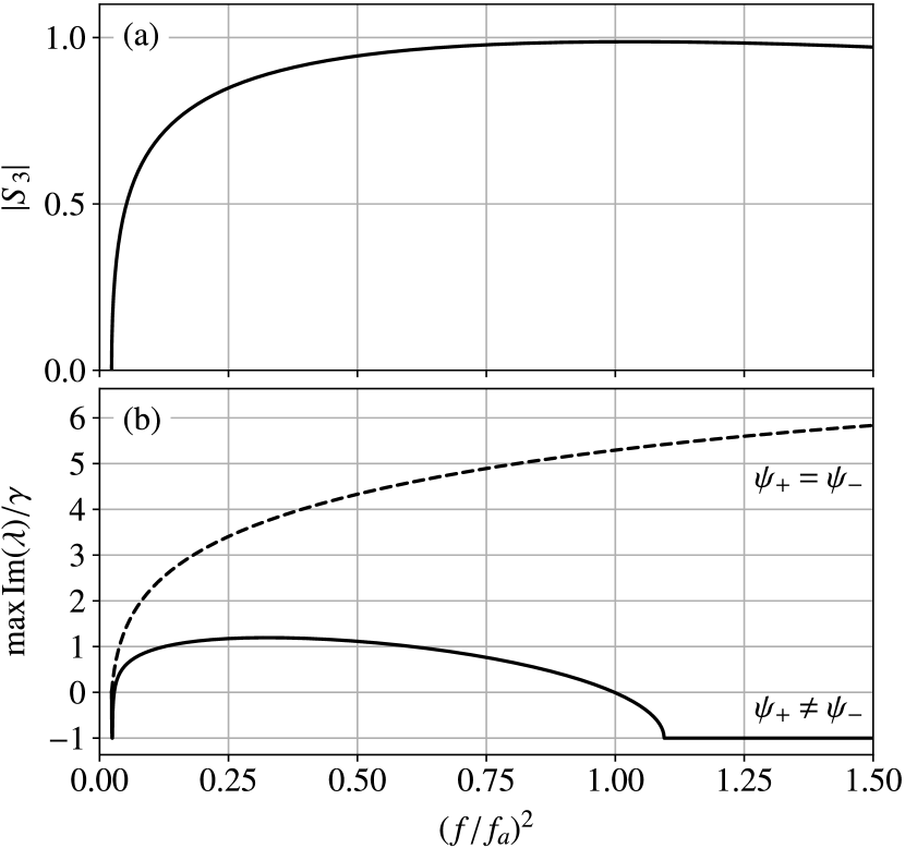
Figure 2: (a) Circular-polarization degree as a function of pump intensity. (b) Corresponding decay rates in the symmetric (dashed line) and main asymmetric (solid line) states of the system. $\lambda$ denotes the eigenvalues of (17). Parameters are the same as in Fig. 1.

Let us find the circular-polarization degree, also referred to as the third Stokes parameter $(S_{3})$. Proceeding from its definition and then using (8) and (7), we have

$$S_{3}=\frac{\mu_{+}-\mu_{-}}{\mu_{+}+\mu_{-}}=\pm\sqrt{1-\frac{4\,\bigl{[}(u-a)^{2}+\gamma^{2}\bigr{]}}{u^{2}}}$$ (16)

in the allowed range of asymmetric states $l_{1}<u<l_{2}$. Notice that $S_{3}(l_{1,2})=0$ [see (9)], so that both limiting points belong to the symmetric branch (15). The maximum of $|S_{3}|$ equals $1-2\gamma^{2}/a^{2}$, given that $\gamma\ll a$, and is reached at $u=a+\gamma^{2}/a$. Figure 2(a) represents the dependence of $|S_{3}|$ on $f^{2}$ for $u$ in a subinterval of $(l_{1},u_{2})$. The system is seen to have nearly total right- or left-handed polarization in a wide range of $f^{2}$ around $f_{a}^{2}=ag^{2}/4V$ (this quantity equals (12) at $u=a$ and $\gamma\to 0$).

In a similar manner one deals with an arbitrary function of $\bar{\psi}_{\pm}$. One calculates $S_{3}$ and then $\mu_{\pm}=(u/2)(1\pm S_{3})$ depending on $u$, after which the relative phase of $\bar{\psi}_{+}$ and $\bar{\psi}_{-}$ is determined using (4) or (11). Any function of $\bar{\psi}_{\pm}$ is thereby expressed in terms of $u$ and also related to $f^{2}$, because $u$ is a single-valued function of $f^{2}$ in the considered domain. Here we employ this procedure to find the spectrum of elementary excitations (also known as Bogolyubov quasiparticles [42, 43]) for a fixed-point state with given $\bar{\psi}_{\pm}$. The eigenenergies and eigenstates of the excitations are determined by the following $4\times 4$ matrix,

$$\mathcal{L}(\bar{\psi}_{\pm})=\begin{pmatrix}E_{p}-i\gamma+2V|\bar{\psi}_{+}|^{2}-D_{\mathbf{k}}&V\bar{\psi}_{+}^{2}&g/2&0\\ -V\bar{\psi}_{+}^{*2}&E_{p}-i\gamma-2V|\bar{\psi}_{+}|^{2}+D_{\mathbf{k}}&0&-g/2\\ g/2&0&E_{p}-i\gamma+2V|\bar{\psi}_{-}|^{2}-D_{\mathbf{k}}&V\bar{\psi}_{-}^{2}\\ 0&-g/2&-V\bar{\psi}_{-}^{*2}&E_{p}-i\gamma-2V|\bar{\psi}_{-}|^{2}+D_{\mathbf{k}}\end{pmatrix},$$ (17)

where $D_{\mathbf{k}}$ means $E_{p}-E_{0}(\mathbf{k})$ for a spatially extended system characterized by the dispersion law $E_{0}(\mathbf{k})$ or merely equals $D$ in the single-mode case. The derivation of (17) from Eq. (1) can be found elsewhere [27, 25, 26]. Solving the characteristic equation $\det(\mathcal{L}(\bar{\psi}_{\pm})-\lambda\mathrm{I})=0$ yields four eigenvalues $\lambda$. The considered fixed-point state is said to be unstable when at least one of them has positive imaginary part for any $\mathbf{k}$, which implies spontaneous growth of infinitesimal fluctuations in the corresponding $k$-state or in the driven mode itself. If, by contrast, all $\mathop{\mathrm{Im}}\lambda$ are negative, fluctuations decay with time and the solution is stable.

Figure 2(b) represents the dependence of $\Gamma=\max\mathop{\mathrm{Im}}\lambda$ on $f^{2}$ in a subinterval of $(l_{1},u_{2})$. It is seen that all symmetric solutions (15) are unstable. In fact, they lose stability already at $u=l_{1}$, where the asymmetric branch originates, and remain unstable until it eventually merges back, which occurs at $u=l_{2}$ and $f^{2}=4f_{a}^{2}$. Thus, when the asymmetric solutions merely exist in accordance with (9), the symmetry is really destroyed in the sense of spontaneously growing fluctuations. Such an “exchange of stabilities” between two branches of fixed points is indicative of the transcritical bifurcation [44]. This kind of transition takes place at $g\geq D$; in the opposite case, the $u=l_{1}$ point is not directly reachable and the transition is discontinuous.

The spin symmetry breakdown under coherent driving was experimentally observed in a microcavity with $g/\gamma\sim 2$, where it resulted in a fast transition from linear to circular polarization of the emitted light [31, 32, 33]. After the symmetry has broken, such a system gets locked in a state with very high $|S_{3}|$ similar to Fig. 2(a), so that a significant increase in pump intensity is required for the transition to the upper symmetric state. Later it was found that the asymmetric solutions may also lose stability, provided that $g/\gamma\gtrsim 4$ [23, 24]. The corresponding Bogolyubov spectra were found analytically in the case when one of two spin components nearly vanishes owing to symmetry breaking [25]. In Fig. 2(b) we draw $\Gamma$ in a wide area of $f$ and now intend to offer a simple qualitative explanation of the presented result. (The explicit formulae for all eigenvalues of (17) are given in Appendix.)

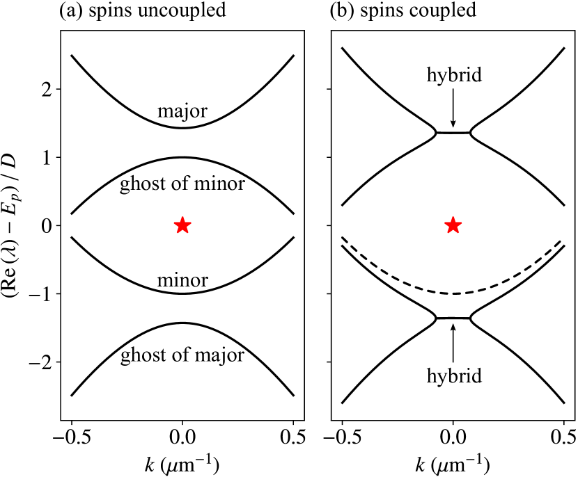
Figure 3: Hybridization of elementary excitations. $\lambda$ denotes the eigenvalues of (17). Parameters in (b) correspond to the asymmetric solution in Fig. 2 at $f=f_{a}$. In (a), all parameters are the same except $g=0$. The dispersion law corresponds to a GaAs-based microcavity.

First, let us take Eq. (1) with $g=0$, so that spins are uncoupled. The excitations are then determined by two $2\times 2$ submatrices of (17). Solving the characteristic equations gives

$$\lambda_{1,2}=E_{p}-i\gamma\mp\sqrt{(D_{\mathbf{k}}-2\mu)^{2}-\mu^{2}}$$ (18)

for each spin component. For the purposes of illustration, consider a spatially extended system with a nearly parabolic dispersion law $E_{0}(k)$ in the vicinity of $k=0$. If $\mu\to 0$, then $\lambda_{1}(k)$ equals $E_{0}(k)-i\gamma$, whereas $\lambda_{2}(k)$ represents the “ghost” branch that originates owing to the pairwise interaction [45, 46]. As $\mu$ is increased, the normal dispersion branch is blueshifted and the ghost branch with $d^{2}E/dk^{2}<0$ is redshifted evenly. Now suppose that one of two spin components is strong and the other is zero; then the normal branch of the major component can be close to resonance with the ghost branch of the minor component and vice versa, which is sketched in Fig. 3(a). If $g=0$, this is nothing but an approximate coincidence of energies; however, a nonzero spin coupling acts to hybridize both resonant pairs below and above the pumped mode as shown in Fig. 3(b). Owing to hybridization, the joint states acquire positive $\Gamma$ and grow spontaneously [26].

The above consideration enables one to estimate the optimal parameters where the instability of the asymmetric states is the most strong. The normal level of the major component is determined by (18) and equals $E_{p}+\sqrt{(D-2\mu)^{2}-\mu^{2}}$, whereas the ghost level of the minor component is $E_{p}+D$ (for $k=0$). The two levels coincide when $3\mu=4D$; then a formal replacement of $\mu$ with $a=D+g/2$ yields $D=3g/2$. Such a relation between $D$ and $g$ leads to nearly optimal hybridization conditions for the “most asymmetric” state with $u\approx a$ even when the spin coupling is introduced fully self-consistently.

Let us turn back to Fig. 2(b) showing the dependence of $\Gamma$ on $f^{2}$ in the asymmetric domain. Since $D=0.9g$, the hybridization conditions are not optimal for $u=a$; namely, the uncoupled major level seen in Fig. 3(a) is noticeably higher than the nearest ghost level. In the discussed example, $\Gamma$ turns to zero at $f\approx 0.999f_{a}$, so that further increasing $f$ cancels the hybridization completely, and, vice versa, decreasing $f$ lowers the major level and thus strengthens its coupling with the ghost one. That is why $\Gamma$ shows an increase with decreasing $f^{2}$ from $f_{a}^{2}$ down to ${\sim}\,0.3f_{a}^{2}$. In the range of small $f^{2}$ around $0.1f_{a}^{2}$, the ghost level is also lowered, which is explained by the population of the minor spin component in view of partially restored symmetry. Since both the major and ghost levels decrease simultaneously, they remain coupled and ensure positive $\Gamma$. As a result, the asymmetric states are unstable until $f^{2}$ becomes as small as ${\sim}\,0.03f_{a}^{2}$.

In summary, we have ascertained that all fixed-point solutions can be unstable in a broad range of pump intensities. The asymmetric solutions change very sharply near the lesser of two $\Gamma=0$ points. By contrast, the greater one, found in the vicinity of $f=f_{a}$ for $D\sim g$, appears to be a “smooth” bifurcation point in which the steady states continuously arise from or turn into the oscillatory states. Such a transition, referred to as the Hopf bifurcation, is analyzed below.

IV Limit cycles

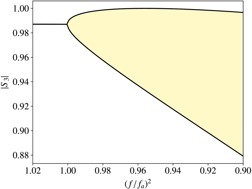
Figure 4: The Hopf bifurcation in the vicinity of $f=f_{a}$. The two lines represent the minimum and maximum of $|S_{3}|$ of an established solution depending on $f$. The initial conditions play no role.

Figure 4 displays a series of numeric solutions of Eqs. (1) in the vicinity of the Hopf bifurcation. The system parameters correspond to Figs. 1 and 2. Since the upper $\Gamma=0$ point of the asymmetric branch is very close to $f_{a}=\sqrt{ag^{2}/4V}$, we keep using the latter quantity as a natural unit of $f$ (in general, the $\Gamma=0$ points are sensitive to $D/g$ and not pinned to $f_{a}$). The series shown in Fig. 4 consists of many independent solutions obtained for different $(f/f_{a})^{2}$ around 1 with a step of $5\times 10^{-4}$. Each solution was recorded after a 100 ns long “establishment” period that largely exceeds the characteristic time of transient processes $\hbar/\gamma$. The results do not depend on the initial conditions, sharp jumps accompanying symmetry breaking and everything else occurred at the early stages of the evolution.

The continuous onset of the oscillations in the $\Gamma=0$ point is not self-evident. In spite of the fact that crossing such points is indeed very likely to result in the second-order phase transitions in lasers [47, 48, 49], the polariton system driven above resonance can behave differently. For instance, the parametric scattering, which starts smoothly while the pumped mode resides at the lower branch of the S-shaped curve, is accompanied by a gradual accumulation of energy under constant external conditions until the system eventually jumps to the upper branch [50, 51, 22]. The considered system, by contrast, has no alternative fixed points it could tend towards, whereas the filling of the hybrid modes does not act to increase the total energy. (Indeed, one of two spin components is suppressed and the other has already reached its higher-energy state, so that an additional blueshift would only worsen resonance conditions for the pumped mode.) Thus, the parametric scattering is inherently balanced for each $f$ in the vicinity of $f=f_{a}$.

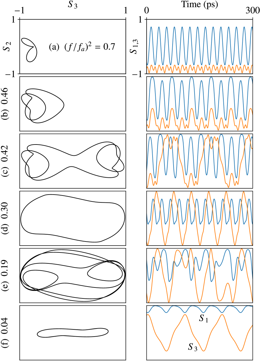
Figure 5: Limit-cycle solutions at different $(f/f_{a})^{2}$. Quantities $S_{1,2,3}$ are the Stokes vector components. The solutions are bistable for (a) and (b) and independent of the initial conditions for (c–f), so that the sole basin of attraction covers the entire phase space.

Let us now decrease $f$ and enter the range of more intensive oscillations. Figure 5 displays the trajectories (left side) and explicit dynamics (right side) in terms of the Stokes vector components $S_{1,2,3}$. Along with the circular-polarization degree $S_{3}$ [(16)], they include

$$S_{1}=\frac{|\psi_{x}|^{2}-|\psi_{y}|^{2}}{|\psi_{x}|^{2}+|\psi_{y}|^{2}},\quad S_{2}=\frac{\psi_{x}^{*}\psi_{y}^{\vphantom{*}}+\psi_{y}^{*}\psi_{x}^{\vphantom{*}}}{|\psi_{x}|^{2}+|\psi_{y}|^{2}}.$$ (19)

$S_{1,2}$ represent the degrees of linear polarization in two spatial bases, $(\mathbf{e}_{x},\mathbf{e}_{y})$ and $\frac{1}{\sqrt{2}}(\mathbf{e}_{x}+\mathbf{e}_{y},\mathbf{e}_{x}-\mathbf{e}_{y})$. In accordance with the usual definition,

$$\dbinom{\psi_{x}}{\psi_{y}}=\frac{1}{\sqrt{2}}\left(\begin{matrix}1&1\\ i&-i\end{matrix}\right)\dbinom{\psi_{+}}{\psi_{-}},$$ (20)

so that all spin-symmetric states with $\psi_{+}=\psi_{-}$ must be polarized along the $x$ axis and have $S_{1}=+1$. The Stokes vector $\mathbf{S}$ defined this way has the length of unity.

Figure 5(a) exemplifies the periodic solutions obtained in a broad range of $(f/f_{a})^{2}$ from 0.9 to 0.5. Apart from growing amplitude, they are qualitatively the same for each $f$. The system is seen to oscillate near the state with circular polarization, either right- or left-handed. Such solutions prove to be stable against weak perturbations and represent two alternative periodic attractors (limit cycles). In a sense, they continue the two respective branches of fixed points.

The amplitude of oscillation grows with decreasing $f$. At $(f/f_{a})^{2}=0.46$ [Fig. 5(b)], the orbit nearly approaches the midpoint of spin domains and becomes more complex; being composed of two different circuits, it shows a doubled period. The next step in decreasing $f$ makes the system enter the opposite domain, which means the possibility of spin switches. Such switches can be chaotic in a certain transitional range of $f$, but eventually the alternative solutions unite and the common orbit runs through both spin domains evenly [Fig. 5(c)]. As $f$ is decreased further, the solution undergoes a sequence of transformations [Figs. 5(d)–(f)], ending up in a fixed-point state with $S_{1}=+1$.

$n$	$-3$	$-2$	$-1$	0	$+1$	$+2$	$+3$
$\mu_{x}/a$	${<}\,10^{-11}$	0.06	${<}\,10^{-11}$	0.52	${<}\,10^{-11}$	0.18	${<}\,10^{-11}$
$\mu_{y}/a$	0.03	${<}\,10^{-11}$	0.35	${<}\,10^{-11}$	0.11	${<}\,10^{-11}$	0.02

Table 1: Discrete spectrum of a periodic solution at $(f/f_{a})^{2}=0.3$ [Fig. 5(d)]. The energy levels are located at $E=E_{p}+n\Delta$, where $\Delta\approx 1.036\,D/2$ and $n$ is integer. Quantities $\mu_{x,y}$ are equal to $V|\psi_{x,y}|^{2}$.

As soon as the opposite solutions unite, the mean values of $|\psi_{+}|$ and $|\psi_{-}|$ become the same. Together with strict periodicity, this gives rise to discrete energy spectra whose individual levels have linear polarizations. Table 1 represents such a spectrum for $(f/f_{a})^{2}=0.3$. The energy dependences were obtained by the Fourier transform of $\psi_{x,y}(t)$ over an interval of 40 ns. All spectral lines, which are fairly unbroadened in view of their “parametric” nature, exhibit alternating linear polarizations oriented along the $x$ and $y$ axes. The behavior of the solution resembles the intrinsic Josephson effect in a system with two orthogonally polarized levels [40, 41, 33], which manifests itself in varying phase difference $\arg(\psi_{x}^{*}\psi_{y}^{\vphantom{*}})$ and, thus, in the oscillations between $S_{2}=\pm 1$ and $S_{3}=\pm 1$, similarly to Fig. 5(d). However, in our case the alternating states are numerous. The higher-order levels get populated through a direct “off-branch” scattering [52, 53] and decay exponentially with increasing $|n|$. By contrast, the peaks listed in Table 1 are the main ones which reflect an inherent balance of instabilities. The difference between adjacent co-polarized levels, $2\Delta$, corresponds to the oscillation period $T=\pi\hbar/\Delta$. Since the total intensity is a very slow function of $f$ in the asymmetric domain, $2\Delta$ is still comparable to $D$ in accordance with Fig. 3, despite the changed polarization states. The solutions shown in Figs. 5(c), (e), and (f) also have unbroadened spectra with alternating $x$ and $y$ levels, but their $\Delta$’s are markedly different because of the period-doubling effect.

All orbits shown in Figs. 5(c)–(f) appear to be the only attractors existing for the respective values of $f$. Each orbit is stable against arbitrary perturbations and does not depend on the initial conditions, which was checked for a broad range of $\psi_{+}$ and $\psi_{-}$. Namely, the initial values of $|\psi_{\pm}|$ were independently varied in the interval from 0 to $1.5\sqrt{a}$ with a step of $0.1\sqrt{a}$, whereas $\arg(\psi_{+}^{*}\psi_{-}^{\vphantom{*}})$ was varied from 0 to $2\pi$ with a step of $0.1\pi$. When the accuracy was sufficiently high, all trajectories for each given $f$ merged into the same orbit.

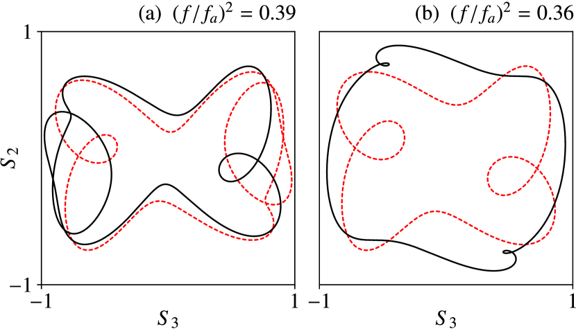
Figure 6: Bistable periodic solutions. The solid and dashed curves (also distinct in color) display alternative trajectories which are chosen depending on the initial conditions.

Being qualitatively different, the absolutely stable orbits are separated by more complex dynamical regimes in the transitional ranges of $f$ (Fig. 6). First, the system can lose the spin symmetry even after the unification of spin domains. As a result, a pair of solutions with broken symmetry become equally possible depending on the initial conditions. One such pair, obtained at $(f/f_{a})^{2}=0.39$, is shown in Fig. 6(a). A less common situation with two spin-symmetric solutions is found at $(f/f_{a})^{2}=0.36$ [Fig. 6(b)]. In both cases the system can be switched between its alternative periodic states using additional pulsed excitation.

Apart from bistable limit cycles, the system displays dynamical chaos. In particular, chaotic solutions are found at $(f/f_{a})^{2}\sim 0.44$, close to the fusion of spin domains, where trajectories are extremely sensitive to fluctuations. The way from Fig. 5(d) to 5(e) also contains a chaotic interval. Specifically, the system loses the spin symmetry in analogy to Fig. 6(a) and then experiences a continuous transition to chaos through a number of the period-doubling events. The initial oscillation period $T_{0}$ is comparable to $2\pi\hbar/D$, similarly to Fig. 5(d). As $f$ is decreased, the period is doubled at certain critical points $f_{i}$, some of which are listed in Table 2.

$i$	1	2	3	4
$T_{i}/T_{0}$	2	4	8	16
$f_{i}^{2}/f_{a}^{2}$	0.2509	0.2426	0.2410	0.24068
$\displaystyle\frac{f_{i-1}^{2}-f_{i-2}^{2}}{f_{i}^{2}-f_{i-1}^{2}}$	—	—	5.19	5.00

Table 2: Several events of period doubling.

At each step, the interval between successive bifurcations becomes $\delta_{i}\approx 5$ times shorter than previously. This behavior is general for one-dimensional discrete chaotic systems such as the logistic map [54]. With increasing $i$, the shortening coefficients $\delta_{i}$ tend to the universal limit $\delta=4.669\!\ldots,$ known as the Feigenbaum constant, that does not depend on a specific system or the choice of its bifurcation parameter. The continuous systems with at least three degrees of freedom demonstrate a wider variety of routes to chaos, but the period-doubling scenario remains one of the most common [55]. It should only be noticed that finding the bifurcation points with high $i$ can be difficult, because it requires a rapidly growing computational accuracy.

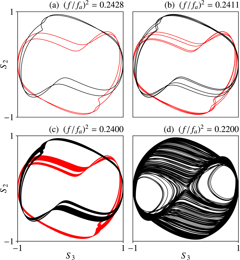
Figure 7: Transition to chaos through a cascade of the period-doubling bifurcations. Different colors in (a)–(c) represent alternative solutions. The time span in (c) and (d) is 10 ns.

Figures 7(a,b) display the solutions obtained after the first and second period-doubling events. The orbits have the correspondingly increased numbers of circuits but remain qualitatively similar. Since the interval between successive bifurcations is small, each newborn pair of circuits cannot diverge very strongly by the moment of the next doubling. The solutions retain self-similarity in spite of many bifurcations even when they become chaotic at $f\lesssim f_{i\,{=}\,\infty}$ [Fig. 7(c)]. As a result, such solutions remain bistable. The alternative chaotic states seen in Fig. 7(c) originate from the same initial conditions as a pair of their respective ancestors at the top of the bifurcation cascade. However, further decreasing $f$ makes the trajectories unite and thus cancels bistability [Fig. 7(d)]. Afterwards, the reverse bifurcation cascade occurs, which comprises successive period halvings, ending up in a state shown in Fig. 5(e). In spite of a complicated orbit, the latter state is particularly stable in a broad range of $(f/f_{a})^{2}$ from 0.19 to 0.09. In other words, a “multiple” periodicity of the trajectory is no longer related to a reduced stability.

Solving Eqs. (1) in a general form is hardly possible. Nevertheless we can explain very roughly, which kind of solutions should be expected depending on $g$ and $D$. The main empirical parameter is the maximum gain rate of the asymmetric fixed points, $\max_{f}\Gamma$. In our examples, it is comparable to $\gamma$ [Fig. 2(b)]. Notice that both $u$ and $\Gamma$ are slow functions of $f$ for the asymmetric branches. At the same time, $\max_{f}\Gamma$ strongly depends on $D/g$ and reaches its own maximum at $D/g\sim 3/2$ (see Sec. III), where it appears to be significantly greater than $\gamma$. In this case the interval of $f$ which contains no stable fixed points is mostly “chaotic”. By contrast, at $D/g\lesssim 0.5$ all nonsteady solutions, if they ever exist, are regular and do not even exhibit bistability. The other “regular” area is found at $D/g\gtrsim 2$. Here, $\Gamma$ is decreased for the usual reason: the hybridization conditions in the sense of Fig. 3 are hampered by a comparatively great energy mismatch of the excitations, but now the upper major level turns out to be too low. This area of $D/g$ has its own interesting features, particularly for the case of a spatially extended system when the hybridization conditions are better satisfied for nonzero wave numbers. At last, the area of $D\sim g$, on which we have been focused in the present work, exhibits several regular and several chaotic intervals of $f$ and thus delivers an especially rich phenomenology.

We have not yet discussed the role played by the ratio $g/\gamma$. It was chosen to be equal to 9 in all examples, but in our general analysis we only supposed it to be indefinitely great. On one hand, this assumption is well justified, because the instability of the asymmetric fixed points is known to be possible for all $g/\gamma\gtrsim 4$ (the greater, the better) [25, 26]. The symmetric states lose stability in the interval $l_{1}<u<l_{2}$ that is also independent of $\gamma$ when $\gamma\ll a$ [see (10)]. At the same time, there exists a different kind of asymmetric solutions, represented by curve $c$ in Fig. 1. It is sensitive to $\gamma$ and completely absent at $\gamma=0$ when the second term in (12) equals zero. Owing to this term, equation $df/du=0$ has an additional root $f=f_{3}$ that determines the beginning point of the respective branch. If $\gamma$ is small compared to $g$ and $D$, then [56]

$$f_{3}^{2}\approx\frac{2\gamma g(g+D)}{V}.$$ (21)

All new solutions with $du/df>0$ are stable; thus, being feasible at a given $f$, they break up the “exclusive” character of limit cycles. The considered case of $g/\gamma=9$ is in fact close to a state in which $f_{3}\propto\sqrt{\gamma}$ becomes less than $f$ at the upper $\Gamma=0$ point of the asymmetric domain for $D\sim g$. When this indeed occurs for a somewhat greater $g/\gamma$, the Hopf bifurcation turns into a more complex discontinuous transition at $f=f_{3}$, which proceeds between the new fixed points and nonzero limit cycles. The new solutions bring about interesting phenomena such as phase bistability; namely, a pair of alternative steady states may have equal polarizations $(\mathbf{S})$ but opposite phases and thus annihilate each other at the places of spatial contact. This leads to a perfectly spontaneous formation of topological excitations (quantized vortices and dark solitons) in spatially extended polariton systems [56].

V Discussion

Among all known polariton systems which show nontrivial dynamics under one-mode driving, the discussed system appears to be the most simple, at least from a conceptual viewpoint. It does not require even the spatial extent and does not rely upon any sort of nonlinear interaction between two coherent components. The very possibility of chaos in this system was doubted in earlier works [28]. Nevertheless, an unexpectedly rich set of nonsteady states, both regular and chaotic, was found.

The reason for the dynamical complexity of the considered system lies in the fact of its spontaneously broken symmetry. The asymmetric fixed points easily lose stability, giving way to nontrivial dynamics. Therefore, the challenge is to find out where exactly the solutions of Eqs. (2)(3) become unstable. In general, the total number of different fixed points that coexist for the same $f$ can reach nine, which makes the whole picture quite complicated. That is why our preceding study [23] did not go far beyond a mere demonstration of oscillatory and chaotic regimes for some particular parameters. In this work, we have found that the intrinsic symmetry of Eqs. (2)(3) enables one to solve them exactly at $f_{+}=f_{-}$ and thus find all critical points for the transitions between the multistable and essentially nonsteady states. The calculation of the $\Gamma=0$ points is performed straightforwardly, based on the energies of elementary excitations derived in Appendix.

As a result, we have investigated nonsteady polariton states in a wide range of system parameters and found several different types of spin oscillations. The first occurs when a pair of asymmetric fixed points turn into infinitesimal limit cycles which thus continuously extend the respective branches of the multistability diagram. In analogy to conventional multistability, the system can be switched between two opposite trajectories by means of a pulsed perturbation of the driving field. Another kind of oscillations comes into being when the spin symmetry is reestablished via unification of opposite limit cycles. The corresponding energy spectra consist of a number of equally spaced unbroadened lines with alternating orthogonal polarizations. These solutions closely resemble the Josephson effect in freely evolving Bose systems. Notice, however, that the main pair of spectral lines corresponds to the Bogolyubov modes rather than polariton eigenlevels, which means that the discussed effect has no linear analogues.

The periodic variation of $S_{3}$ (average spin) covers almost the whole range from $-1$ to $+1$. Such states with a “dynamical” spin symmetry can be completely independent of the initial conditions and robust against any temporal perturbations. At the same time, they remain very sensitive to the continuous-wave excitation parameters and, for instance, exhibit discrete switches, doublings or halvings, of the oscillation period upon varying $f$. Being highly controllable already on the scale of $10^{2}$ ps (in GaAs-based samples), this type of coherent states can be used for information encoding and transmission. Finally, we have found that in a certain range of pump amplitudes the system experiences a deterministic and continuous transition to chaos through an infinite cascade of period doublings. The chaotic variation of $S_{3}$ represents an extremely fast analogue of the polarization chaos formerly observed in electrically driven laser diodes [58, 59, 60].

For simplicity, our study has been restricted to the case of zero-dimensional polariton systems in micropillars. At the same time, the analysis of the fixed points and their bifurcations remains valid in a more general case of laterally uniform cavities. Owing to the spatial extent, the simultaneous instability of all plane-wave solutions for a given $f$ can result in spontaneous ordering, spatiotemporal oscillations or chaos, and chimera states in which ordered and disordered subsystems coexist [23, 24, 26, 56]. A precise spin symmetry and homogeneity of the model enable one to solve the steady-state equations analytically but do not constitute rigid requirements to the experimental conditions. However, a significant strength of the spin coupling compared to the decay rate $(g/\gamma>4)$ remains necessary, still being a challenging task for experimental realization.

Appendix A Explicit formulae for energies of elementary excitations

Here we calculate the eigenvalues of (17) for all steady states obeying Eqs. (2), (3). Owing to the intrinsic symmetry of the equations, one can reduce this multiparameter problem to a single free variable. The results apply to both a pointlike micropillar and a homogeneous cavity in which a plane-wave polariton condensate is excited at $\mathbf{k}=0$. In the latter case, $D_{\mathbf{k}}$ means $E_{p}-E_{0}(\mathbf{k})$, where $E_{0}(\mathbf{k})$ is the usual dispersion law of polaritons.

The characteristic equation for (17), $\det(\mathcal{L}(\bar{\psi}_{\pm})-\lambda\mathrm{I})=0$, has the following roots,

$$\lambda=E_{p}-i\gamma\pm\sqrt{\frac{P\pm\sqrt{Q}}{2}},$$ (22)

where

$$P =3(\mu_{+}^{2}+\mu_{-}^{2})-4D_{\mathbf{k}}(\mu_{+}+\mu_{-})+2D_{\mathbf{k}}^{2}+\frac{g^{2}}{2},$$ (23)

$$Q =g^{2}\left\{4\left[D_{\mathbf{k}}-(\mu_{+}+\mu_{-})\right]^{2}-(\mu_{+}+\mu_{-})^{2}+4\mu_{+}\mu_{-}\cos^{2}\varphi\right\}$$

$$+(\mu_{+}-\mu_{-})^{2}\left[4D_{\mathbf{k}}-3(\mu_{+}+\mu_{-})\right]^{2},$$ (24)

$\mu_{\pm}=V|\bar{\psi}_{\pm}|^{2}$, and $\varphi=\arg(\bar{\psi}_{+}^{*}\bar{\psi}_{-}^{\vphantom{+}})$. To obtain $\cos\varphi$ for $\bar{\psi}_{+}\neq\bar{\psi}_{-}$, recall that (11) can be unambiguously expressed in terms of $u=\mu_{+}+\mu_{-}$ and $w=\sqrt{\mu_{+}\mu_{-}}$; this leads to

$$w\cos\varphi=a-u+\frac{2\gamma^{2}}{2a-u}.$$ (25)

(In case of multimode systems, quantity $a$ corresponds to the driven mode, i. e., $a\equiv D_{\mathbf{k}\,{=}\,0}+g/2$.) We assume that $l_{1}<u<l_{2}$ and employ Eq. (7), which enables us to rewrite all functions of $\mu_{+}$, $\mu_{-}$, and $\varphi$ in terms of only one “condensate” variable, $u$. As a result, (22) takes the following general form for the states with spontaneously broken symmetry,

$$\lambda^{\mathrm{(a)}}=E_{p}-i\gamma\pm\frac{1}{\sqrt{2}}\Biggl{\{}2(D_{\mathbf{k}}-u)^{2}+u^{2}-6(a-u)^{2}-6\gamma^{2}+\frac{g^{2}}{2}\\ {}\pm\Biggl{[}(u^{2}-4(a-u)^{2}-4\gamma^{2})(4D_{\mathbf{k}}-3u)^{2}+4g^{2}(D_{\mathbf{k}}-u)^{2}-g^{2}u^{2}\\ {}+4g^{2}\left(a-u+\frac{2\gamma^{2}}{2a-u}\right)^{2}\Biggr{]}^{1/2}\Biggr{\}}^{1/2}.$$ (26)

A characteristic example for $\mathop{\mathrm{Re}}\lambda^{\mathrm{(a)}}(k)$ is shown in Fig. 3(b). An approximate particular case of (26), obtained for the state in which one of two spin components is exactly zero, was considered earlier in Refs. [25, 24].

In order to find the excitations for the spin-symmetric solutions, one should set $\varphi=0$ and $\mu_{+}=\mu_{-}=u/2$ in (23), (24), which yields

$$\lambda^{\mathrm{(s)}}=E_{p}-i\gamma\pm\frac{1}{2}\sqrt{[2(D_{\mathbf{k}}-u)\pm g]^{2}-u^{2}}.$$ (27)

As expected, expressions (26) and (27) become exactly the same in both limiting points $u=l_{1,2}$.

The two signs of $g$ in the radicand of Eq. (27) correspond to a pair of orthogonally polarized states (e. g., the plus sign leads to an effective $D^{\prime}=D+g/2$ which is the pump detuning from the lower resonance level having the $y$ polarization, thus, the respective Bogolyubov modes are also $y$-polarized). When $u=l_{1}$, the degenerate solutions $\lambda^{(\mathrm{s},y)}$ and $\lambda^{\mathrm{(a)}}$ have exactly zero $\Gamma\equiv\max\mathop{\mathrm{Im}}\lambda$. This quantity becomes negative at $u>l_{1}$ for $\lambda^{\mathrm{(a)}}$ and positive for $\lambda^{(\mathrm{s},y)}$, which implies spontaneous growth of the $y$-polarized Bogolyubov excitations on the background of the $x$-polarized condensate and necessarily leads to the spin symmetry breaking. If $g>D$, then the $u=l_{1}$ point lies on a stable branch with a positive slope $(du/df>0)$, so that the polarization transition at $f=f(l_{1})$ occurs continuously.

References

- Kavokin et al. [2017] A. V. Kavokin, J. J. Baumberg, G. Malpuech, and P. Laussy, Microcavities, 2nd ed. (Oxford University Press, New York, 2017).
- Baas et al. [2006] A. Baas, J.-P. Karr, M. Romanelli, A. Bramati, and E. Giacobino, Quantum Degeneracy of Microcavity Polaritons, Phys. Rev. Lett. 96, 176401 (2006).
- Elesin and Kopaev [1973] V. F. Elesin and Y. V. Kopaev, Bose condensation of excitons in a strong electromagnetic field, Sov. Phys. JETP 36, 767 (1973).
- Keldysh [2017] L. V. Keldysh, Coherent states of excitons, Phys. Usp. 60, 1180 (2017).
- Baas et al. [2004] A. Baas, J. P. Karr, H. Eleuch, and E. Giacobino, Optical bistability in semiconductor microcavities, Phys. Rev. A 69, 023809 (2004).
- Gippius et al. [2004] N. A. Gippius, S. G. Tikhodeev, V. D. Kulakovskii, D. N. Krizhanovskii, and A. I. Tartakovskii, Nonlinear dynamics of polariton scattering in semiconductor microcavity: Bistability vs. stimulated scattering, Europhys. Lett. 67, 997 (2004).
- Carusotto and Ciuti [2004] I. Carusotto and C. Ciuti, Probing Microcavity Polariton Superfluidity through Resonant Rayleigh Scattering, Phys. Rev. Lett. 93, 166401 (2004).
- Gavrilov et al. [2007] S. S. Gavrilov, N. A. Gippius, V. D. Kulakovskii, and S. G. Tikhodeev, Hard mode of stimulated scattering in the system of quasi-two-dimensional exciton polaritons, JETP 104, 715 (2007).
- Gippius et al. [2007] N. A. Gippius, I. A. Shelykh, D. D. Solnyshkov, S. S. Gavrilov, Y. G. Rubo, A. V. Kavokin, S. G. Tikhodeev, and G. Malpuech, Polarization Multistability of Cavity Polaritons, Phys. Rev. Lett. 98, 236401 (2007).
- Shelykh et al. [2008a] I. A. Shelykh, T. C. H. Liew, and A. V. Kavokin, Spin Rings in Semiconductor Microcavities, Phys. Rev. Lett. 100, 116401 (2008a).
- Gavrilov et al. [2010] S. S. Gavrilov, N. A. Gippius, S. G. Tikhodeev, and V. D. Kulakovskii, Multistability of the optical response in a system of quasi-two-dimensional exciton polaritons, JETP 110, 825 (2010).
- Paraïso et al. [2010] T. K. Paraïso, M. Wouters, Y. Léger, F. Morier-Genoud, and B. Deveaud-Plédran, Multistability of a coherent spin ensemble in a semiconductor microcavity, Nat. Mater. 9, 655 (2010).
- Sarkar et al. [2010] D. Sarkar, S. S. Gavrilov, M. Sich, J. H. Quilter, R. A. Bradley, N. A. Gippius, K. Guda, V. D. Kulakovskii, M. S. Skolnick, and D. N. Krizhanovskii, Polarization Bistability and Resultant Spin Rings in Semiconductor Microcavities, Phys. Rev. Lett. 105, 216402 (2010).
- Adrados et al. [2010] C. Adrados, A. Amo, T. C. H. Liew, R. Hivet, R. Houdré, E. Giacobino, A. V. Kavokin, and A. Bramati, Spin Rings in Bistable Planar Semiconductor Microcavities, Phys. Rev. Lett. 105, 216403 (2010).
- Gavrilov et al. [2012] S. S. Gavrilov, A. S. Brichkin, A. A. Demenev, A. A. Dorodnyy, S. I. Novikov, V. D. Kulakovskii, S. G. Tikhodeev, and N. A. Gippius, Bistability and nonequilibrium transitions in the system of cavity polaritons under nanosecond-long resonant excitation, Phys. Rev. B 85, 075319 (2012).
- Ballarini et al. [2013] D. Ballarini, M. De Giorgi, E. Cancellieri, R. Houdré, E. Giacobino, R. Cingolani, A. Bramati, G. Gigli, and D. Sanvitto, All-optical polariton transistor, Nat. Commun. 4, 1778 (2013).
- Cerna et al. [2013] R. Cerna, Y. Léger, T. K. Paraïso, M. Wouters, F. Morier-Genoud, M. T. Portella-Oberli, and B. Deveaud, Ultrafast tristable spin memory of a coherent polariton gas, Nat. Commun. 4, 2008 (2013).
- Carusotto and Ciuti [2013] I. Carusotto and C. Ciuti, Quantum fluids of light, Rev. Mod. Phys. 85, 299 (2013).
- Krizhanovskii et al. [2010] D. N. Krizhanovskii, D. M. Whittaker, R. A. Bradley, K. Guda, D. Sarkar, D. Sanvitto, L. Viña, E. Cerda, P. Santos, K. Biermann, R. Hey, and M. S. Skolnick, Effect of Interactions on Vortices in a Nonequilibrium Polariton Condensate, Phys. Rev. Lett. 104, 126402 (2010).
- Pigeon et al. [2011] S. Pigeon, I. Carusotto, and C. Ciuti, Hydrodynamic nucleation of vortices and solitons in a resonantly excited polariton superfluid, Phys. Rev. B 83, 144513 (2011).
- Claude et al. [2020] F. Claude, S. V. Koniakhin, A. Maître, S. Pigeon, G. Lerario, D. D. Stupin, Q. Glorieux, E. Giacobino, D. Solnyshkov, G. Malpuech, and A. Bramati, Taming the snake instabilities in a polariton superfluid, Optica 7, 1660 (2020).
- Gavrilov [2021] S. S. Gavrilov, Loop parametric scattering of cavity polaritons, Phys. Rev. B 103, 184304 (2021).
- Gavrilov [2016] S. S. Gavrilov, Towards spin turbulence of light: Spontaneous disorder and chaos in cavity-polariton systems, Phys. Rev. B 94, 195310 (2016).
- Gavrilov [2018] S. S. Gavrilov, Polariton Chimeras: Bose-Einstein Condensates with Intrinsic Chaoticity and Spontaneous Long-Range Ordering, Phys. Rev. Lett. 120, 033901 (2018).
- Gavrilov [2017] S. S. Gavrilov, On a new mechanism of polariton-polariton scattering, JETP Lett. 105, 200 (2017).
- Gavrilov [2020a] S. S. Gavrilov, Nonequilibrium transitions, chaos, and chimera states in exciton-polariton systems, Phys. Usp. 63, 123 (2020a).
- Sarchi et al. [2008] D. Sarchi, I. Carusotto, M. Wouters, and V. Savona, Coherent dynamics and parametric instabilities of microcavity polaritons in double-well systems, Phys. Rev. B 77, 125324 (2008).
- Solnyshkov et al. [2009] D. D. Solnyshkov, R. Johne, I. A. Shelykh, and G. Malpuech, Chaotic Josephson oscillations of exciton-polaritons and their applications, Phys. Rev. B 80, 235303 (2009).
- Leblanc et al. [2020] C. Leblanc, G. Malpuech, and D. D. Solnyshkov, High-frequency exciton-polariton clock generator, Phys. Rev. B 101, 115418 (2020).
- Chestnov et al. [2021] I. Chestnov, Y. G. Rubo, A. Nalitov, and A. Kavokin, Pseudoconservative dynamics of coupled polariton condensates, Phys. Rev. Research 3, 033187 (2021).
- Gavrilov et al. [2013] S. S. Gavrilov, A. V. Sekretenko, S. I. Novikov, C. Schneider, S. Höfling, M. Kamp, A. Forchel, and V. D. Kulakovskii, Polariton multistability and fast linear-to-circular polarization conversion in planar microcavities with lowered symmetry, Appl. Phys. Lett. 102, 011104 (2013).
- Sekretenko et al. [2013] A. V. Sekretenko, S. S. Gavrilov, S. I. Novikov, V. D. Kulakovskii, S. Höfling, C. Schneider, M. Kamp, and A. Forchel, Spin and density patterns of polariton condensates resonantly excited in strained planar microcavities with a nonuniform potential landscape, Phys. Rev. B 88, 205302 (2013).
- Gavrilov et al. [2014] S. S. Gavrilov, A. S. Brichkin, S. I. Novikov, S. Höfling, C. Schneider, M. Kamp, A. Forchel, and V. D. Kulakovskii, Nonlinear route to intrinsic Josephson oscillations in spinor cavity-polariton condensates, Phys. Rev. B 90, 235309 (2014).
- Josephson [1962] B. Josephson, Possible new effects in superconductive tunnelling, Phys. Lett. 1, 251 (1962).
- Cataliotti et al. [2001] F. S. Cataliotti, S. Burger, C. Fort, P. Maddaloni, F. Minardi, A. Trombettoni, A. Smerzi, and M. Inguscio, Josephson Junction Arrays with Bose-Einstein Condensates, Science 293, 843 (2001).
- Levy et al. [2007] S. Levy, E. Lahoud, I. Shomroni, and J. Steinhauer, The a.c. and d.c. Josephson effects in a Bose-Einstein condensate, Nature 449, 579 (2007).
- Lagoudakis et al. [2010] K. G. Lagoudakis, B. Pietka, M. Wouters, R. André, and B. Deveaud-Plédran, Coherent Oscillations in an Exciton-Polariton Josephson Junction, Phys. Rev. Lett. 105, 120403 (2010).
- Abbarchi et al. [2013] M. Abbarchi, A. Amo, V. G. Sala, D. D. Solnyshkov, H. Flayac, L. Ferrier, I. Sagnes, E. Galopin, A. Lemaître, G. Malpuech, and J. Bloch, Macroscopic quantum self-trapping and Josephson oscillations of exciton polaritons, Nat. Phys. 9, 275 (2013).
- Ohadi et al. [2016] H. Ohadi, Y. del Valle-Inclan Redondo, A. Dreismann, Y. G. Rubo, F. Pinsker, S. I. Tsintzos, Z. Hatzopoulos, P. G. Savvidis, and J. J. Baumberg, Tunable Magnetic Alignment between Trapped Exciton-Polariton Condensates, Phys. Rev. Lett. 116, 106403 (2016).
- Shelykh et al. [2008b] I. A. Shelykh, D. D. Solnyshkov, G. Pavlovic, and G. Malpuech, Josephson effects in condensates of excitons and exciton polaritons, Phys. Rev. B 78, 041302(R) (2008b).
- Shelykh et al. [2010] I. A. Shelykh, A. V. Kavokin, Y. G. Rubo, T. C. H. Liew, and G. Malpuech, Polariton polarization-sensitive phenomena in planar semiconductor microcavities, Semicond. Sci. Technol. 25, 013001 (2010).
- Bogolyubov [1947] N. N. Bogolyubov, On the theory of superfluidity, J. Phys. (USSR) 11, 23 (1947), [Izv. Akad. Nauk SSSR, Ser. Fiz. 11, 77 (1947)].
- Pitaevskii and Stringari [2016] L. Pitaevskii and S. Stringari, Bose-Einstein Condensation and Superfluidity (Oxford University Press, New York, 2016).
- Strogatz [2015] S. H. Strogatz, Nonlinear dynamics and chaos, 2nd ed. (CRC Press, 2015).
- Kohnle et al. [2011] V. Kohnle, Y. Léger, M. Wouters, M. Richard, M. T. Portella-Oberli, and B. Deveaud-Plédran, From Single Particle to Superfluid Excitations in a Dissipative Polariton Gas, Phys. Rev. Lett. 106, 255302 (2011).
- Stepanov et al. [2019] P. Stepanov, I. Amelio, J.-G. Rousset, J. Bloch, A. Lemaître, A. Amo, A. Minguzzi, I. Carusotto, and M. Richard, Dispersion relation of the collective excitations in a resonantly driven polariton fluid, Nat. Commun. 10, 3869 (2019).
- Haken [1975] H. Haken, Analogy between higher instabilities in fluids and lasers, Phys. Lett. A 53, 77 (1975).
- Haken [1983] H. Haken, Synergetics, An Introduction. Nonequilibrium Phase Transitions & Self-Organization in Physics, Chemistry & Biology (Springer, 1983).
- Cross and Hohenberg [1993] M. C. Cross and P. C. Hohenberg, Pattern formation outside of equilibrium, Rev. Mod. Phys. 65, 851 (1993).
- Gavrilov [2014] S. S. Gavrilov, Blowup dynamics of coherently driven polariton condensates, Phys. Rev. B 90, 205303 (2014).
- Gavrilov et al. [2015] S. S. Gavrilov, A. S. Brichkin, Y. V. Grishina, C. Schneider, S. Höfling, and V. D. Kulakovskii, Blowup dynamics of coherently driven polariton condensates: Experiment, Phys. Rev. B 92, 205312 (2015).
- Savvidis et al. [2001] P. G. Savvidis, C. Ciuti, J. J. Baumberg, D. M. Whittaker, M. S. Skolnick, and J. S. Roberts, Off-branch polaritons and multiple scattering in semiconductor microcavities, Phys. Rev. B 64, 075311 (2001).
- Whittaker [2005] D. M. Whittaker, Effects of polariton-energy renormalization in the microcavity optical parametric oscillator, Phys. Rev. B 71, 115301 (2005).
- Feigenbaum [1978] M. J. Feigenbaum, Quantitative universality for a class of nonlinear transformations, J. Stat. Phys. 19, 25 (1978).
- Bohr et al. [1998] T. Bohr, M. H. Jensen, G. Paladin, and A. Vulpiani, Dynamical Systems Approach to Turbulence (Cambridge University Press, 1998).
- Gavrilov [2020b] S. S. Gavrilov, Spontaneous formation of vortices and gray solitons in a spinor polariton fluid under coherent driving, Phys. Rev. B 102, 104307 (2020b).
- Note [1] The derivation of in Ref. [56] was based on a different approximation that led to . In turn, formula (21) is based on Eq. (12) and represents an exact solution of the equation at .
- Virte et al. [2013a] M. Virte, K. Panajotov, H. Thienpont, and M. Sciamanna, Deterministic polarization chaos from a laser diode, Nat. Photonics 7, 60 (2013a).
- Virte et al. [2013b] M. Virte, K. Panajotov, and M. Sciamanna, Bifurcation to nonlinear polarization dynamics and chaos in vertical-cavity surface-emitting lasers, Phys. Rev. A 87, 013834 (2013b).
- Sciamanna and Shore [2015] M. Sciamanna and K. A. Shore, Physics and applications of laser diode chaos, Nat. Photonics 9, 151 (2015).