Extensible Logging and
Empirical Attainment Function
for IOHexperimenter

Abstract

In order to allow for large-scale, landscape-aware, per-instance algorithm selection, a benchmarking platform software is key. IOHexperimenter provides a large set of synthetic problems, a logging system and a fast implementation.

In this work, we refactor IOHexperimenter’s logging system, in order to make it more extensible and modular. Using this new system, we implement a new logger, which aim at computing performance metrics of an algorithm across a benchmark. The logger computes the most generic view on an anytime stochastic heuristic performances, in the form of the Empirical Attainment Function (EAF). We also provide some common statistics on the EAF and its discrete counterpart, the Empirical Attainment Histogram.

Our work has eventually been merged in the IOHexperimenter codebase.

1 Introduction

IOHexperimenter [Doerr et al., 2018] is a framework for the benchmarking of anytime stochastic heuristics for optimization problems that holds together a set of benchmarks and an advanced logging system. It provides Pseudo-Boolean Optimization problem generators (PBO) and the Black-Box Optimization Benchmark (BBOB). Its core is implemented in C++, which allow for fast computations, a crucial feature for benchmarking on synthetic problems.

One of the most notable feature of IOHexperimenter is its logging system. A so-called Logger target an automated export of the algorithms’ behaviour in a standardized format, which can be seamlessly imported in the IOHanalyzer for further study. It most notably allows for tracking the states of the algorithms’ parameters, a unique feature on the market of benchmarking platforms.

The legacy logging system was implemented as a single class, exposing a set of hard-coded parameters which controlled when logging event occurred, what parameters were to be watched and how they would be stored in a set of CSV files.

The limitations of the legacy system were:

• The logging event list was not extensible.

• Only plain floating-point parameters could be logged.

• Parameters had to be explicitly sent by the calling solver and should always exists.

• It was only possible to log into the IOHanalyzer format, in a set of CSV text files.

We show in section 2 how we remove those limitations.

The new logging system is also more extensible and allows for easiest implementation of new loggers. This feature allowed us to add a new logger which targets immediate performance estimation, so as to help for automated algorithm selection. By binding the optimized problems and the performance estimation of a solver in a single binary, we allow for very fast benchmarking runs.

Having fast benchmarking is a crucial feature for allowing per-instance algorithm configuration. As shown in [Aziz-Alaoui et al., 2021], having the performance estimation directly bound to the solver’s binary allows for configuration budget that are an order of magnitude larger than other approaches.

In a previous work, we implemented an IOHexperimenter logger which efficiently computes the discrete version of the empirical attainment function on a linear scale. In this work, we refactor this logger, adding log scales, and add a logger computing the empirical attainment function itself, as explained in section 3. We also refactored the debugging tools within IOHexperimenter, by using the Clutchlog project, which allow for fine-grained management of debug messages.

2 Logging System Architecture

Instead of a monolithic Logger, we design a set of modular classes, as shown on Figure 1.

Figure 1: UML class diagram of the architecture that we implemented for the logging system.

A Logger is thus most notably composed as two objects:

Trigger:

given the context at call, returns true if the call event is to be logged (cf. Section 2.1),

Property:

gives access to what value should be logged (cf. Section 2.2),

Subclassing from the Logger interface allow to design a fully configurable object, with user-defined Triggers and Properties. For instance, the Watcher class allows the user to specify which Properties to watch. The standardized logging system for IOHanalyzer is itself defined as a sub-class of Watcher.

We add a Logger object that allow for combining several loggers into a single one: Combine. For instance, this wrapper is useful if one want to computes a global performance and save the whole run. This system allow to assemble Loggers at run time.

2.1 Triggers

The Triggers are functors which can be called on the LogInfo context and returns a boolean, stating if a log event should be triggered.

The sets of available Triggers is straightforward and matches the previous features, they allow to log an event:

Always:

triggers an event at every objective function call,

OnImprovement:

if the given solution has a better objective function value than the previous best one,

At:

at the given set of objective function call indices,

Each:

at regular intervals,

During:

during the given sets of objective function call intervals,

Instead of managing those Triggers all at once, we allow to aggregate them with triggers that behaves like logical operators:

Any:

trigger an event if any of the managed Trigger instances is triggered,

All:

trigger an event if all of the managed Trigger instances is triggered.

⬇

1problem::MetaData pb(0,0,"fake",2);

2logger::Info i;

3i.transformed_y = 9999;

4

5trigger::OnImprovement t;

6

7// First call.

8EXPECT_TRUE(t(i,pb)); // Better than infinity.

9

10i.transformed_y = 100;

11EXPECT_TRUE(t(i,pb)); // Improvement.

12EXPECT_FALSE(t(i,pb)); // Strict inequality.

13

14// Improvement.

15i.transformed_y = 10;

16EXPECT_TRUE(t(i,pb)); // Improvement.

17EXPECT_FALSE(t(i,pb)); // Strict inequality.

18

19// Unsuspected increasing.

20i.transformed_y = 99;

21EXPECT_FALSE(t(i,pb)); // Not improving.

22

23// Internal state stability.

24i.transformed_y = 11;

25EXPECT_FALSE(t(i,pb)); // Still worst than internal test.

26

27i.transformed_y = 9;

28EXPECT_TRUE(t(i,pb)); // Better than internal state.

29

30t.reset();

31i.transformed_y = 99;

32EXPECT_TRUE(t(i,pb)); // Better than infinity.

Listing 1: Excerpt of the code used to test the behaviour of the OnImprovement Trigger.

2.2 Properties

A Property is a way to access a value of interest, which can be either a state of the IOHexperimenter context or an external variable of interest.

The set of available Properties accessing the context matches the previous features:

Evaluations:

the number of calls to the objective function so far,

YBest:

the best objective function value found so far,

TransformedY:

the current objective function value, with invariant-testing transformation(s) applied,

TransformedYBest:

the best transformed value found so far.

We add a set of classes to help accessing several kind of external variables, which targets any algorithm parameter:

Reference:

capture a reference to a variable,

Pointer:

capture a pointer to a variable,

PointerReference:

capture a pointer to a reference to a variable.

The two last classes allow for indicating if the Property is existing (or not) in the current context. This is useful for dynamic algorithm configuration, for which a given parameter may exists only for some variant.

For instance, if one is logging the state of an algorithm that switch its mutation operator, some of those operators may have various parameters. Those parameters would be available only if this specific operator is actually instantiated.

The low-level interface uses C++’s standard library’s std::optional feature to indicate if this Property is available in this context. Pointer-based capturing classes are provided as a generic way to interact with any code, as it is sufficient to set the pointer to nullptr to indicate that a Property is disabled in the current context.

⬇

1using namespace ioh;

2

3suite::BBOB suite({1, 2}, {1, 2}, {3, 10}); // problems, instances, dimensions

4

5// Properties that watch my_attribute:

6double my_attribute = 0;

7watch::Reference attr("Att_reference", my_attribute);

8watch::Pointer attp("Att_pointer" ,&my_attribute);

9double* p_transient_att = nullptr;

10watch::PointerReference attpr("Att_PtrRef", p_transient_att);

11

12// Instantiate some properties:

13trigger::Always always;

14watch::Evaluations evaluations;

15watch::RawYBest raw_y_best;

16watch::TransformedY transformed_y;

17watch::TransformedYBest transformed_y_best;

18

19logger::Store logger({always},

20 // Attach those properties to the logger:

21 {evaluations, raw_y_best, transformed_y, transformed_y_best, attr, attp, attpr});

22suite.attach_logger(logger);

23

24/* [Call the problem function…] */

25

26// One can select which metadata layer to consider:

27logger::Store::Cursor first_eval(suite.name(), /*pb*/1, /*dim*/3, /*ins*/1, /*run*/0, /*eval*/0);

28

29// And recover a property value at this event:

30auto evals = logger.at(first_eval, evaluations);

Listing 2: Excerpt of code used to test the behaviour of some context Properties.

2.3 Debugging Messages

We refactor the legacy debug messaging system, replacing it with a set of macros using the Clutchlog library. This allows to (de)clutch messages for a given: log level, source code location or call stack depth. Additionally, the unit tests interface use this features, which can be used from the command line interface.

⬇

1$ ./test_eaf --gtest_filter=*eaf_logger Note ".*eaf\.hpp"

2[...]

3[test_eaf] N:>>>>>>>>>>>>>>>> Attach to: pb=1, dim=10, ins=1, run=0 attach_problem @ eaf.hpp:245

4[test_eaf] N:>>>>>>>>>>>>> reset reset @ eaf.hpp:289

5[test_eaf] N:>>>>>>>>>>>>> Attach to: pb=1, dim=10, ins=1, run=1 attach_problem @ eaf.hpp:245

6[test_eaf] N:>>>>>>>>>>>>> reset reset @ eaf.hpp:289

7[...]

8[test_eaf] N:>>>>>>>>>>>>> Attach to: pb=2, dim=30, ins=2, run=1 attach_problem @ eaf.hpp:245

9[test_eaf] N:>>>>>>>>>>>>> reset reset @ eaf.hpp:289

10[test_eaf] N:>>>>>>>>>>>>> Attach to: pb=2, dim=30, ins=2, run=2 attach_problem @ eaf.hpp:245

11

12$ ./test_eaf --gtest_filter=*eaf_logger Debug ".*eaf.*"

13[...]

14[test_eaf] D:>>>>>>>>>>> Attach suite BBOB to logger TestBody @ test_eaf.cpp:16

15[test_eaf] N:>>>>>>>>>>>>>>>> Attach to: pb=1, dim=10, ins=1, run=0 attach_problem @ eaf.hpp:245

16[test_eaf] I:>>>>>>>>>>> pb:1, dim:10, ins:1 TestBody @ test_eaf.cpp:20

17[test_eaf] I:>>>>>>>>>>> > run:0 TestBody @ test_eaf.cpp:22

18[test_eaf] D:>>>>>>>>>>>>>> EAF called after improvement call @ eaf.hpp:265

19[test_eaf] N:>>>>>>>>>>>>> reset reset @ eaf.hpp:289

20[test_eaf] N:>>>>>>>>>>>>> Attach to: pb=1, dim=10, ins=1, run=1 attach_problem @ eaf.hpp:245

21[...]

22test_eaf] I:>>>>>>>>>>> Result fronts: TestBody @ test_eaf.cpp:34

23[test_eaf] I:>>>>>>>>>>> > Front size=1 TestBody @ test_eaf.cpp:45

24[test_eaf] I:>>>>>>>>>>> > Front size=1 TestBody @ test_eaf.cpp:45

25[test_eaf] I:>>>>>>>>>>> > Front size=2 TestBody @ test_eaf.cpp:45

26[...]

27[test_eaf] I:>>>>>>>>>>> > Front size=4 TestBody @ test_eaf.cpp:45

Listing 3: Examples of debugging messages tuning, upper part shows messages up to the Note level for eaf.hpp file, lower part shows messages up to the Debug level for any file containing the eaf word.

3 Empirical Attainment Loggers

In order to allow for large-scale algorithm configuration, we aim at having a performance evaluation within the solver executable, so as to ease its interfacing with automated configurators. IOHexperimenter, providing both the benchmark problems and a logging system, is a good candidate to host a performance logger. However, there is many ways of looking at the performance of stochastic heuristics. In this work, we wanted to implement the most generic one, so as to allow the user to use various performance metrics. Figure 2 shows why we think that the Empirical Attainment Function (EAF) is the most generic choice in the case of synthetic benchmarking.

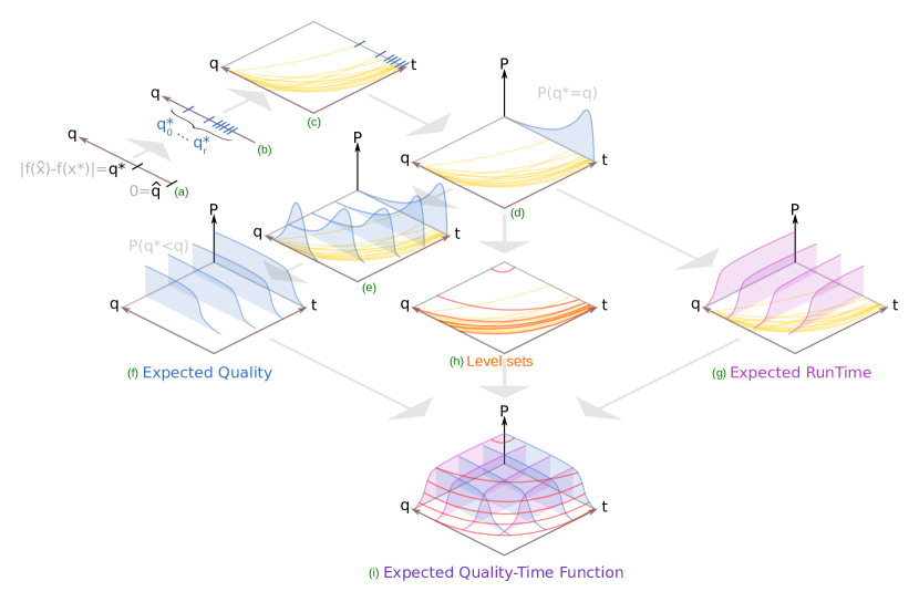
Figure 2: A classical way of looking at the performance is to look at the objective function value as the error (“quality” $q^{*}$) to a known bound $\hat{q}$, after a given “time” budget (a). For randomized algorithm, a statistic over the qualities output by several runs should be considered (b). But stochastic searches are anytime, hence showing monotonic “attainment trajectories” of best-so-far values along the time axis (c). A classical setting is to compute a performance statistic over the end distribution (d). From those two quality and time axis, one can consider several distribution along the time one (e), most generally in the form of cumulative distribution (f) showing the expected quality for given budgets. Conversely, one can consider the expected run time for given qualities (g), which is one of the most popular setting. Additionally, one can consider 2D first-order moments of the 2D quality/time distribution of trajectories (h). This forms a 2D distribution, called the Empirical Attainment Function (i).

Section 3.1 introduces how the EAF can be viewed as the Empirical Cumulative Distribution Function (ECDF) of 2D objective function values’ attainment trajectories, and how it can be discretized into an Empirical Attainment Histogram (EAH).

3.1 Empirical Cumulative Distribution Functions

This section introduces the ECDF of points and then generalize this notion to attainment trajectories, up to the EAF and EAH. Table 1 introduces the notation used in this section.

Table 1: Notation.

$i,n\in\mathbb{N}$	integers
$x,y\in\mathbb{R}$	scalar real values
$\mathbf{x},\mathbf{z}\in\mathbb{R}^{2}$	points (vectors) in 2D space
$\mathcal{X},\mathcal{Y}$	scalar real random variables
$Z,L\subset\mathbb{R}^{2}$	sets of points
$A=\{Z_{1},\dotsc,Z_{n}\}$	collection, i.e., a multiset of sets
$\mathds{1}(\cdot)$	Indicator function that returns $\{0,1\}$
$\mathbf{z}_{1}\preceq\mathbf{z}_{2}$	point $\mathbf{z}_{1}$ weakly dominates point $\mathbf{z}_{2}$
$Z\preceq\mathbf{z}$	at least one point $\mathbf{z}\in Z$ weakly dominates point $\mathbf{z}$

3.1.1 Of points — ECDF

Let $(\mathcal{X}_{1},\dotsc,\mathcal{X}_{n})$ be independent, identically distributed real random variables with the common cumulative distribution function $F(x)$. Then, the Empirical Cumulative Distribution Function (ECDF) is classicaly [Van der Vaart, 1998, p. 265] defined as:

$$\widehat{F}^{n}(x)=\frac{1}{n}\sum_{i=1}^{n}\mathds{1}(x_{i}\leq x)$$ (1)

where $\mathds{1}(\cdot)$ is the indicator function that returns 0 or 1 and $x_{i}\sim\mathcal{X}_{i}$.

For a pair of random variables $\mathcal{Q}$, $\mathcal{T}$, the joint ECDF is given by:

$$\widehat{F}^{n}(q,t)=\frac{1}{n}\sum_{i=1}^{n}\mathds{1}(q_{i}\leq q\land t_{i}\leq t)$$ (2)

where $q_{i}$ and $t_{i}$ are samples from random variables $\mathcal{Q}$ and $\mathcal{T}$, respectively.

Let $\mathbf{a}\preceq\mathbf{b}\iff\mathbf{a}^{d}\leq\mathbf{b}^{d}\ \forall d\in\mathbb{N}^{+}$ denote the weak dominance of a $d$-dimensional point $\mathbf{a}$ over point $\mathbf{b}$.

For a set of points $Y=\{\mathbf{y}_{0},\dots,\mathbf{y}_{n}\}$ (e.g. with $\mathbf{y}=\{q,t\}$), the joint ECDF becomes:

$$\widehat{F}^{n}(\mathbf{y})=\frac{1}{n}\sum_{i=1}^{n}\mathds{1}(Y_{i}\preceq\mathbf{y})$$ (3)

3.1.2 Of trajectories — EAF

Let $Z=\{Y_{0},\dots,Y_{m}\}$ be a set of non-dominated set of $\mathbf{y}$ points (e.g. $\mathbf{y}=\{q,t\}$). Note that a set $Y\in Z$ can weakly dominate another set $\{\mathbf{y}\}$ of cardinality one.

The “Empirical Attainment Function” [Grunert da Fonseca et al., 2001] is defined as the ECDF of the closed set $Z$, over $\mathbf{y}$ [Grunert da Fonseca and Fonseca, 2002]:

$$\widehat{G}^{m}(\mathbf{y})=\frac{1}{m}\sum_{i=1}^{m}\mathds{1}(Z_{i}\preceq\mathbf{y})$$ (4)

3.1.3 Discretization as Histograms

One can without loss of generality use a function $h:\mathbb{R}^{d}\mapsto\mathbb{R}^{d}$ which may discretize the input space, and consider a generic set $R$ of size $r$ on which element the domination operator can be applied to compare it to any point $\mathbf{y}$:

$$\widehat{G}^{r}_{h}(\mathbf{y})=\frac{1}{r}\sum_{i=1}^{r}\mathds{1}(R_{i}\preceq h(\mathbf{y}))$$ (5)

3.2 2D Quality/Time Distributions

The Quality/Time EAF can be defined as eq. 5 with $h(\mathbf{y})=\mathbf{y}$ and $R=Z=\{Y_{0},\dots,Y_{m}\}$, a set of “attainment trajectories”. In our case, a trajectory is a set of weakly non-dominated $\{q,t\}$ points, being the best quality/time targets encountered by the optimization algorithm.

The Empirical Attainment Histogram (EAH) can be defined as eq. 5, using $R=Z$ and a discretization function:

$$h(\mathbf{y})=\Delta^{-1}\left(\left\lfloor\Delta(\mathbf{y})\right\rfloor\right)$$ (6)

A linear discretization of the histograms can be defined by mapping on $\mathbb{N}^{+}$, as an indexed space, useful for implementation:

$$\Delta_{\beta}(\mathbf{y})=\left(\mathbf{y}-\mathbf{v}\right)\frac{\beta}{l}$$ (7)

leading to:

$$h_{\beta}(\mathbf{y})=\left\lfloor\left(\mathbf{y}-\mathbf{v}\right)\frac{\beta}{l}\right\rfloor\frac{l}{\beta}+\mathbf{v}$$ (8)

where $\beta$ is the number of buckets of the histogram, $\mathbf{v}=\min(Y)$, the minimum corner of Y and $l=|\max(Y)-\mathbf{v}|$.

Similarly, a log-discretization can be defined with:

$$\Delta_{\beta}(\mathbf{y})=\frac{\beta\cdot\log\left(1+\left(\mathbf{y}-\mathbf{v}\right)\right)}{\log(1+l)}$$ (9)

leading to:

$$h_{\beta}(\mathbf{y})=\exp\left(\left(\left\lfloor\frac{\beta\cdot\log\left(1+\left(\mathbf{y}-\mathbf{v}\right)\right)}{\log(1+l)}\right\rfloor+1\right)\frac{\log(1+l)}{\beta}\right)-1+\mathbf{v}$$ (10)

3.3 Algorithms

To compute the EAF, we use the algorithm of [Fonseca et al., 2011], and follow the implementation provided by [López-Ibáñez et al., 2010], which is available in the eaf package fo R. In short, the algorithm computes the level sets of attainment points $\{q,t\}$, as figured by the red lines in Figure 2 (h) and (i).

Note that the algorithm to compute the log-EAH is adapted from [Knowles, 2005], using the log discretization function 10.

3.4 Implementation

The implementation takes the form of the EAF class, inheriting from the Logger while fixing the Properties that are watched and the Triggers to the one being necessary to the EAF computation (YBest and OnImprovement, respectively).

As we want the user to be able to compute various statistics over the EAF, we store every level set in a separated vector, storing the metadata about the run with which they have been produced. Each EAF is thus attached to the run, the problem instance, the dimension and the suite for which it has been produced. This allow the user to operate any aggregation across metadata and compute any statistics.

We provide several generic statistics in the form of computation of the Surface of a given attainment level, and the Volume of a given set of levels. The user can use low-level classes to indicate which Nadir point they want to use, if the default worst point is not desired.

Note that the volume gives access to a first-order moment-like statistic that behave like the average, while the surface of the median level of the EAF gives access to a robust, median-like statistics. Second-order moment statistics may be computed, as explained in [Fonseca et al., 2005]. Additionally, it would be possible to take (or aggregate) slice(s) of the EAF in order to recover expected runtime or expected quality distributions.

⬇

1size_t sample_size = 10;

2size_t nb_runs = 10;

3suite::BBOB suite({1, 2}, {1, 2}, {10, 30});

4// Instantiate the EAF logger.

5logger::EAF logger;

6suite.attach_logger(logger);

7

8// Classical benchmark calls:

9for(const auto& pb : suite) {

10 for(size_t r = 0; r < nb_runs; ++r) {

11 for(size_t s = 0; s < sample_size; ++s) {

12 (*pb)(common::random::pbo::uniform(

13 static_cast<size_t>(pb->meta_data().n_variables),

14 static_cast<long>(s)));

15 }

16 pb->reset();

17 }

18}

19// Get some EAF levels:

20logger::eaf::Levels levels_at(common::OptimizationType::Minimization, {0, nb_runs/2, nb_runs-1});

21auto levels = levels_at(logger);

Listing 4: Excerpt of code used to test the behaviour of the EAF logger.

The discretized EAHs (for linear scales, as defined in Section 3.2) have been implemented in a previous work and have been ported to the new architecture. We add support for log scales, which are usually more suited to the convex shape of the EAH.

All implemented classes are accompanied by several corresponding unit tests and an extensive documentation, as shown on Figure 3.

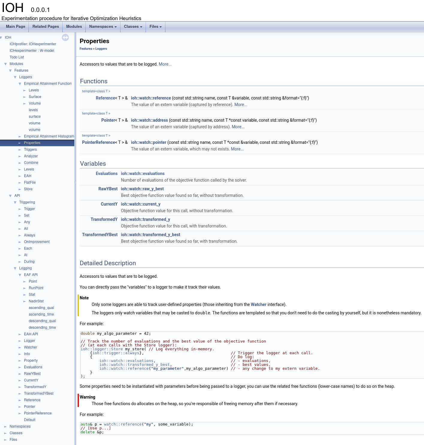
Figure 3: Screenshot of the automatically generated documentation.

4 Conclusion

In this work, we target the use of IOHexperimenter as a key framework for landscape-aware algorithm selection. In order to be able to perform large-scale per-instance automated configuration, we need to embed a powerful logger within a solver executable. Additionally, the logger need to be able to computes various performance statistics across large benchmarks.

So as to allow for a generic performance estimation, we implement the computation of the Quality/Time Empirical Attainment Function, a generalization of Empirical Cumulative Distribution Function for attainment trajectories of anytime stochastic algorithms.

To meet this objective, we refactor the logging system of IOHexperimenter, so as to obtain a highly modular and extensible architecture, with fine-grained debugging message management. Using this new system, we implement the EAF logger and some statistics on this distribution. The new setup have been successfully tested on an extension of our previous work [Dreo et al., 2021].

Our implementation provides an extensive documentation and several examples in the form of unit tests. It has eventually been merged within the IOHexperimenter code base.

References

- [Aziz-Alaoui et al., 2021] Aziz-Alaoui, A., Doerr, C., and Dreo, J. (2021). Towards Large Scale Automated Algorithm Design by Integrating Modular Benchmarking Frameworks. arXiv [cs-NE], 2102.06435.
- [Doerr et al., 2018] Doerr, C., Wang, H., Ye, F., van Rijn, S., and Bäck, T. (2018). IOHprofiler: A Benchmarking and Profiling Tool for Iterative Optimization Heuristics. arXiv [cs-NE], 1810.05281.
- [Dreo et al., 2021] Dreo, J., Doerr, C., Aziz-Alaoui, A., and Zheng, A. (2021). Using irace, paradiseo and iohprofiler for large-scale algorithm configuration. In COnfiguration and SElection of ALgorithms Workshop.
- [Fonseca et al., 2005] Fonseca, C. M., da Fonseca, V. G., and Paquete, L. (2005). Exploring the Performance of Stochastic Multiobjective Optimisers with the Second-Order Attainment Function. In Coello Coello, C. A., Hernández Aguirre, A., and Zitzler, E., editors, Evolutionary Multi-Criterion Optimization, Lecture Notes in Computer Science, pages 250–264, Berlin, Heidelberg. Springer.
- [Fonseca et al., 2011] Fonseca, C. M., Guerreiro, A. P., López-Ibáñez, M., and Paquete, L. (2011). On the Computation of the Empirical Attainment Function. In Takahashi, R. H. C., Deb, K., Wanner, E. F., and Greco, S., editors, Evolutionary Multi-Criterion Optimization, Lecture Notes in Computer Science, pages 106–120, Berlin, Heidelberg. Springer.
- [Grunert da Fonseca and Fonseca, 2002] Grunert da Fonseca, V. and Fonseca, C. M. (2002). A link between the multivariate cumulative distribution function and the hitting function for random closed sets. Statistics & Probability Letters, 57(2):179–182.
- [Grunert da Fonseca et al., 2001] Grunert da Fonseca, V., Fonseca, C. M., and Hall, A. O. (2001). Inferential Performance Assessment of Stochastic Optimisers and the Attainment Function. In Zitzler, E., Thiele, L., Deb, K., Coello Coello, C. A., and Corne, D., editors, Evolutionary Multi-Criterion Optimization, Lecture Notes in Computer Science, pages 213–225, Berlin, Heidelberg. Springer.
- [Knowles, 2005] Knowles, J. (2005). A summary-attainment-surface plotting method for visualizing the performance of stochastic multiobjective optimizers. In 5th International Conference on Intelligent Systems Design and Applications (ISDA’05), pages 552–557.
- [López-Ibáñez et al., 2010] López-Ibáñez, M., Paquete, L., and Stützle, T. (2010). Exploratory Analysis of Stochastic Local Search Algorithms in Biobjective Optimization. pages 209–222. Springer, Berlin, Heidelberg.
- [Van der Vaart, 1998] Van der Vaart, A. W. (1998). Asymptotic statistics. Cambridge university press.