Unusual wave-packet spreading and entanglement dynamics in non-Hermitian disordered many-body systems

Abstract

Non-Hermiticity and dephasing, collaborating in a unusual wave packet dynamics, realizes unconventional entanglement evolution in a disordered, interacting and asymmetric (non-reciprocal) quantum media. Taking the Hatano-Nelson model as a concrete example, we first consider how wave packet spreads in a non-Hermitian disordered system for demonstraing that it is very different from the Hermitian case. Interestingly, a cascade like wave packet spreading as in the Hermitian case is suppressed in the clean limit and at weak disorder, while it revives in the vicinity of the localization-delocalization transition. Based on this observation, we then analyze how the entanglement entropy of the system evolves in the interacting non-Hermitian model, revealing its non-monotonic evolution in time. We clarify the different roles of dephasing in the time evolution of entanglement entropy in Hermitian and non-Hermitian systems, and show that the many-body dynamics is governed by a principle different from the Hermitian case. The size dependence of the results suggests with the increase of disorder, a unusual area-volume-area law crossover of the maximal entanglement entropy. To analyze the effects of disorder on a firm basis, using the Hermitian limit as a benchmark, we employ a quasi-periodic disorder (Aubry-André model) in the analyses.

I Introduction

The entanglement entropy has proven to be one of the useful measures for characterizing many-body localization (MBL) Gornyi et al. (2005); Basko et al. (2006) both in its static Bauer and Nayak (2013); Luitz et al. (2015); Khemani et al. (2017); Kjäll et al. (2014); Serbyn et al. (2016) and dynamical properties.Žnidarič et al. (2008); Bardarson et al. (2012); Serbyn et al. (2013); Agarwal et al. (2015); Bar Lev et al. (2015); Luitz et al. (2016) The MBL phase appears quite generically; i.e., both in theoriesNandkishore and Huse (2015); Alet and Laflorencie (2018); Abanin et al. (2019) and in experimentsSchreiber et al. (2015); Choi et al. (2016); Roushan et al. (2017); Smith et al. (2016); Xu et al. (2018), in disordered (interacting) many-body systems, constituting a counterexample to the eigenstate thermalization hypothesis (ETH),Deutsch (1991); Srednicki (1994); Rigol et al. (2008) the quantum mechanical version of ergodicity. Disorder tends to localize the wave function; cf. Anderson localization in the non-interacting limit, while here in an interacting system the so-called quasi local integrals of motion (LIOMs) Ros et al. (2015); Imbrie et al. (2017) play the roles of localized wave functions in an Anderson insulator. Anderson localizationAnderson (1958) occurs in real space, while MBL manifests in Fock spaceAltshuler et al. (1997); Roy et al. (2019); Roy and Logan (2020); Orito and Imura (2021) due to the emergence of LIOMs. Many-body wave functions in the MBL phase take the form of a simple product in the basis of LIOMs,Ros et al. (2015); Orito and Imura (2021) leading to a strong suppression of entanglement entropy; i.e., the area-law behavior, Bauer and Nayak (2013); Luitz et al. (2015); Khemani et al. (2017) manifesting a sharp contrast to the standard (ergodic) volume law in the ETH phase.

In addition to such a volume-to-area law crossover at the ETH-MBL transition, the entanglement entropy also shows a unique dynamics in the MBL phase; Žnidarič et al. (2008); Bardarson et al. (2012); Serbyn et al. (2013) in the quench dynamics the entanglement entropy stays constant on average after an initial growth in the non-interacting case, [see e.g., Fig. 7, panel (i-a)] while in the MBL phase, it shows a peculiarly slow (typically logarithmic in time) but unbounded growth in the MBL phase (case of $V\neq 0$), reflecting the fact the wave functions (LIOMs) are exponentially localized but the information can still flow; Serbyn et al. (2013); Huse et al. (2014) [see e.g., Fig. 10, panel (i-a)]. The initial growth is mainly due to the increase of the number entropy $S_{\rm num}$, while the subsequent logarithmic growth stems the configuration entropy $S_{\rm conf}$ [see Eqs. (34) and (35) for definitions of $S_{\rm num}$ and $S_{\rm conf}$; cf. Sec. III.1 for details]. Physically, the increase of $S_{\rm num}$ is due to spreading of the wave packet, while dephasing also contributes to the increase of $S_{\rm conf}$. In spreading of the wave packet the focus is on the amplitude of the wave function, while in dephasing it is on the phase of the wave function. To be precise, dephasing occurs only in interacting many-body systems. Also, $S_{\rm num}$ is local, while $S_{\rm conf}$ is non-local in real space. Thus, the entanglement entropy $S_{\rm tot}=S_{\rm num}+S_{\rm conf}$ measures both (i) the relaxation of the initial state due to wave packet spreading, and (ii) the growth of quantum correlation in the process of dephasing.

So far we have in mind the standard Hermitian ETH-MBL systems, while the behavior of entanglement entropy in non-Hermitian systems with non-reciprocal (or asymmetric) hopping Hatano and Nelson (1996, 1997) $\Gamma_{L}=e^{g}\Gamma_{0}$ vs. $\Gamma_{R}=e^{-g}\Gamma_{0}$ [$g$ is the degree of non-reciprocity; see also Eqs. (1), (21)], has been also of some interest recently. It has been reported in Refs. Hamazaki et al., 2019; Zhai et al., 2020; Panda and Banerjee, 2020 that the entanglement entropy $S_{\rm tot}(t)$ shows a non-monotonic time evolution; i.e., at some specific parameter setting the entanglement entropy $S_{\rm tot}(t)$ turns to decrease after its initial growth. Such a non-monotonic behavior of $S_{\rm tot}(t)$ has been attributed to the presence of a finite imaginary part in the eigenvalues $E$ which typically appears in this system; when ${\rm\ Im}E\neq 0$, the wave function is extended and is sensitive to the non-reciprocality of the hopping. On contrary, in the MBL phase the entanglement entropy $S_{\rm tot}(t)$ converges to a single value after some duration. Hamazaki et al. (2019) In spite of these preceding studies (Refs. Hamazaki et al., 2019; Zhai et al., 2020; Panda and Banerjee, 2020) there still remains some open issues; a comprehensive understanding of the various behaviors of $S_{\rm tot}(t)$ at different parameter settings seem to be lacking. Here, in this work we perform a systematic study of $S_{\rm tot}(t)$ in non-Hermitian systems with non-reciprocal hopping, and reveals the nature of its intricate behaviors that differ significantly from those in Hermitian systems. We point out that another factor underlying the difference in the behaviors of $S_{\rm tot}(t)$ in the Hermitian and non-Hermitian systems is a very different way how a wave packet spreads in the two systems.

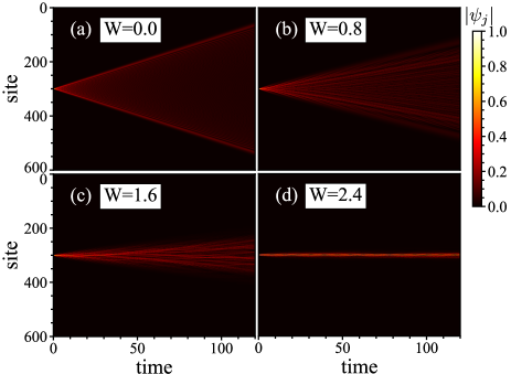
Figure 1: Single-particle dynamics in the Hermitian case: $g=0$. Time evolution of the initial wave packet: $\psi_{j}(0)=\delta_{j,j_{0}}$ is visualized. The amplitude $|\psi_{j}(t)|$ [cf. Eq. (8)] is shown by a gradation of plot colors indicated in the color bar. The abscissa represents time $t$, and the ordinate the site $j$. Different panels (a-d) correspond to different values of disorder strength $W$; $W=0.0,0.8,1.6,2.4$, respectively, for panels (a-d). $\theta_{0}$ is fixed at $\theta_{0}=0$. No disorder averaging. $j_{0}=300$, $L=601$.

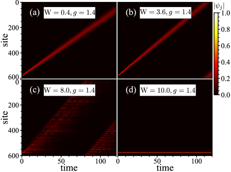
Figure 2: Single-particle dynamics in the non-Hermitian case: $g=1.4$. Time evolution of the initial wave packet under the same condition as in Fig. 1. Here, the values of disorder strength $W$ are such that $W=0.4,3.6,8.0,10.0$, respectively, for panels (a-d). $\theta_{0}=0$, $j_{0}=580$, and $L=601$.

It has recently been pointed out Longhi (2021) that the wave-packet spreading in non-Hermitian systems with non-reciprocal hopping shows very different features. In the presence of a finite non-reciprocity $g$ in hopping the standard “cascade-like” wave-packet spreading [see Fig. 1, panel (a)] in the Hermitian limit $g=0$ becomes extinct. It only revives in the vicinity of the localization transition: $W\simeq W_{c}$ [see Fig. 2, panel (c)]. In the extended phase: $W<W_{c}$, the wave packet does not spread, but it only slides in the direction imposed by the non-reciprocality $g$. In the body of the paper we show and study systematically how this drastic change in the manner of wave-packet spreading caused by the non-reciprocity $g$ is reflected in the dynamical property of the entanglement entropy.

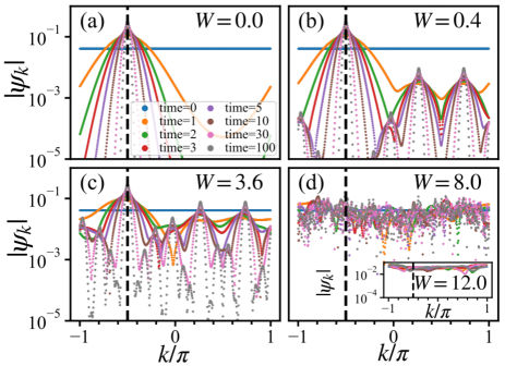
Figure 3: Single-particle dynamics; profile of the wave function in $k$-space. The Fourier transform $|\psi_{k}(t)|$ [Eq. (10)] of the wave packet is plotted as a function of $k$ at different time slices $t=0,1,2,3,5,30,100$ as indicated in the inset of panel (a). Different panels (a-d) and the inset of panel (d) correspond, respectively, to different values of disorder strength $W=0,0.4,3.6,8.0,12.0$. $g$ is fixed at $g=1.4$. $\theta_{0}=0$ (no disorder average). Other settings follow those of Fig. 2.

As already mentioned in the Hermitian limit, the inter-particle interaction $V$ plays a non-trivial role in determining the dynamical property of the entanglement entropy; especially, its effect is predominant in long time-scale dynamics. Here, we show in this paper that the inter-particle interaction $V$ plays also a non-trivial and principal role in the entanglement dynamics of a non-Hermitian system with non-reciprocal hopping. The remainder of the paper is structured as follows. In Sec. II we describe the model and show the mechanics of unusual dynamics. In Sec. III we give details of the entanglement dynamics, highlighting its non-monotonic time evolution. In Sec. IV we examine the size dependence of the results, predicting an unusual area-volume-area law crossover of the maximal entanglement entropy. In Sec. V we point out and visualize the characteristic stages in the evolution of the reduced density matrix, which underlie the unusual non-Hermitian entanglement dynamics. Sec. VI is devoted to concluding remarks. Some details are left to the appendices.

II Spreading of a wave packet in non-Hermitian systems with non-reciprocal hopping

II.1 Single-particle case: Hatano-Nelson $\times$ Aubry-André model

Let us consider the following one-dimensional tight-binding model with non-reciprocal hopping amplitudes $\Gamma_{L},\Gamma_{R}$ (Hatano-Nelson model):Hatano and Nelson (1996)

$$H = -\sum_{j=0}^{L-1}\Big{(}\Gamma_{R}|j+1\rangle\langle j|+\Gamma_{L}|j\rangle\langle j+1|\Big{)}$$ (1)

$$+ W_{j}\sum_{j=0}^{L-1}|j\rangle\langle j|,$$

where $\Gamma_{L}=e^{g}\Gamma_{0}$, $\Gamma_{R}=e^{-g}\Gamma_{0}$ with $g$ being a parameter quantifying the degree of non-reciprocity. $g$ is also sometimes regarded as an imaginary vector potential. Hatano and Nelson (1996) $|j\rangle$ represents a single-particle state localized at site $j$. In the first two (hopping) terms we have chosen the boundary condition to be periodic: $|L\rangle\equiv|0\rangle$. In the third term, we have chosen the on-site potential $W_{j}$ to be quasi-periodic:

$$W_{j}=W\cos(2\pi\theta j+\theta_{0}),$$ (2)

playing effectively the role of a random potential (Aubry-André modelAubry and André (1980)), where $\theta$ is an irrational constant, which we choose to be the so-called (inverse) golden ratio: $\theta=(\sqrt{5}-1)/2$. $\theta_{0}$ is an additive phase introduced for the purpose of taking a disorder average; averaging over $\theta_{0}$ distributed uniformly in the range $\in[0,2\pi)$ plays effectively the role of averaging over different disorder configurations.

In the Hermitian limit: $g=0$, the eigenstates are extended when $W$ is weak enough ($W<W_{c}$), while localized for $W>W_{c}$, where

$${W_{c}\over 2\Gamma_{0}}=1.$$ (3)

This may be understood from the behavior of localization length $\xi$ defined in the localized phase; Longhi (2021); De Tomasi et al. (2021) i.e.,

$$\xi^{-1}\simeq\log{W\over 2\Gamma}.$$ (4)

The localization length $\xi$ diverges as $W$ approaches the critical value (3) from above.

In the non-Hermitian case: $g\neq 0$, the delocalization point is determined by the condition:Hatano and Nelson (1997); Heußen et al. (2021)

$$\xi^{-1}=g>0.$$ (5)

If this is combined with Eq. (4), the delocalization transition is expected to occur at

$$W=W_{c}=2\Gamma_{0}\ e^{g}=2\Gamma_{L},$$ (6)

where we have assumed $\Gamma_{L}>\Gamma_{R}$ ($g>0$); i.e., $W_{c}$ in the non-Hermitian case is found simply by replacing $\Gamma_{0}$ in Eq. (3) with the right/large hopping amplitude $\Gamma_{0}$. Both in the Hermitian and non-Hermitian cases, the location of the mobility edge (6) does not depend on the energy $\epsilon_{n}$; $H|n\rangle=\epsilon_{n}|n\rangle$. When $g\neq 0$, the eigenenergy $\epsilon_{n}$ becomes complex in the extended phase ($W<W_{c}=2\Gamma_{L}$); cf. the case of free particle motion described in Appendix B, while it remains real in the localized phase ($W>W_{c}$). Thus, the localization-delocalization transition is accompanied by a real-complex transition of the eigenenergies (see Appendix A for details).

Let us focus on the dynamics of the system by following how an initially localized wave packet evolves in time. Four panels of Figs. 1 and 2 show examples of such dynamics. We assume that at $t=0$ the wave packet is just at an initial site $j=j_{0}$;

$$|\psi(t=0)\rangle=|j_{0}\rangle.$$ (7)

At time $t$, the wave packet may evolve as

$$|\psi(t)\rangle = \sum_{j}\psi_{j}(t)|j\rangle$$ (8)

$$= \sum_{n}c_{n}e^{-i\epsilon_{n}t}|n\rangle,$$

where $|n\rangle$ represents the $n$th single-particle eigenstate of the Hamiltonian (1) with an eigenenergy $\epsilon_{n}$; i.e., $H|n\rangle=\epsilon_{n}|n\rangle$, while $c_{n}=\langle\langle n|\psi(t=0)\rangle$. Here, $\langle\langle n|$ represents the left eigenstate corresponding to the eigenenergy $\epsilon_{n}$ : $\langle\langle n|H=\epsilon_{n}\langle\langle n|$ and not $|n\rangle^{\dagger}$; $\langle\langle n|\neq|n\rangle^{\dagger}$. We make sure that the left and right eigenstates satisfy the biorthogonal condition, i.e., $\langle\langle n|m\rangle=\delta_{n,m}$. In case of $g\neq 0$, the eigenenergy $\epsilon_{n}$ is typically complex; cf. the free particle case in Appendix B [see also Eqs. (14), (15)], so that the time-evolved wave packet $|\psi(t)\rangle$ literally as given in Eq. (8) tends to grow exponentially; its norm $\langle\psi(t)|\psi(t)\rangle$ is not conserved due to the contribution from states with Im $\epsilon_{n}>0$. In the actual computation, we, therefore, rescale (renormalize) $|\psi(t)\rangle$ at every interval $\Delta t$ as

$$|\psi(t)\rangle\rightarrow|\tilde{\psi}(t)\rangle={|\psi(t)\rangle\over\sqrt{\langle\psi(t)|\psi(t)\rangle}}.$$ (9)

and avoid this computational difficulty.Hamazaki et al. (2019); Zhai et al. (2020)

Let us first consider the Hermitian case. The four panels of Fig. 1 show the distribution of $|\psi_{j}(t)|$ in the case of Hermite case for different strength of $W$. At site $j$ (the abscissa) and at time $t$ (the ordinate), the amplitude of $|\psi_{j}(t)|$ is specified by a variation of the plot color indicated in the color bar. In the clean limit [Fig. 1(a)], the wave packet spreads symmetrically in the two directions. As the strength $W$ of disorder increases (Fig. 1(b), (c)), spreading of the wave packet tends to become slower. Finally, beyond the critical disorder strength (Fig. 1(d)), the wave packet ceases to spread. Then, the four panels of Fig. 2 show the distribution of $|\psi_{j}(t)|$ in the case of $g=1.4$ ($L=601$, $j_{0}=580$) for different strength of $W$. Unlike in the Hermitian case (Fig. 1) the four panels show that the wave packet does not spread; at least in the regime of weak $W$ [cases of panels (a-b)], but rather slides in the direction imposed by the non-reciprocity $g$. In the non-Hermitian case $g\neq 0$ the standard cascade-like wave packet spreading as in the Hermitian limit disappears in the regime of weak $W$ [panels (a-b)] such that $W\ll W_{c}$,Longhi (2021) but a similar (cascade-like) behavior reappears in the vicinity of the localization transition: $W\simeq W_{c}$ [panel (c)]. In the localized phase, the wave packet does not move [panel (d)]. Comparing the three cases on the delocalized side [panels (a-c)], one also notices that the “sliding velocity” of the wave packet; at least the velocity of the wave front $v_{f}$, tends to increase as $W$ is increased.Longhi (2021)

To understand why in the non-Hermitian system the wave-packet dynamics becomes very different from the standard Hermitian case, one may well start with the clean limit: $W=0$. In this limit, the eigenstates are plane waves $\langle j|k\rangle=e^{ikj}/\sqrt{L}$ so that

$$|\psi(t)\rangle = \sum_{k}e^{-i\epsilon_{k}t}|k\rangle\langle k|j_{0}\rangle\left(\equiv\sum_{k}\psi_{k}(t)|k\rangle\right)$$ (10)

$$= \frac{1}{\sqrt{L}}\sum_{j}\sum_{k}e^{-i\epsilon_{k}t+ik(j_{0}-j)}|j\rangle,$$

i.e., $|\psi(t)\rangle$ is generally expressed as a superposition of such plane waves; at site $j$ contributions from different $k$ add up with a phase factor

$$e^{i\phi(k)}=e^{-i\epsilon_{k}t+ik(j_{0}-j)}.$$ (11)

At $t=0$ and at $j\neq j_{0}$, such contributions are out of phase and cancel each other, while at $j=j_{0}$ they add up in phase to form the peak of the initial wave packet. At $t>0$, similarly, the only non-vanishing contributions [in the summation over $k$ in Eq. (10)] are those from the neighborhood of $k=\overline{k}$ at which the phase $\phi(k)$ becomes stationary; i.e., $\phi^{\prime}(\overline{k})=0$, or

$$2\Gamma_{0}\sin\overline{k}\ t=j-j_{0}.$$ (12)

Since $|\sin\overline{k}|\leq 1$, $|j-j_{0}|=2\Gamma_{0}t\equiv v_{f}t$ defines the position of the wave front, or a “light cone”. Longhi (2021) In the Hermitian limit the initially localized wave packet spreads linearly in time: $\Delta x(t)\propto t$; i.e., $\Delta x(t)\sim t^{\sigma}$ with the exponent $\sigma\simeq 1$, where

$$\Delta x(t)=\sqrt{\sum_{j}(j-j_{0})^{2}|\psi_{j}(t)|^{2}}.$$ (13)

represents the spread of the light cone. Addition of disorder $W$ suppresses the wave-packet spreading; as shown in Fig. 2 of Ref. Longhi, 2021, the velocity $v=\Delta x(t)/t$, characterizing the speed of the spreading of wave packet is shown to decrease linearly with $W$ and vanishes at $W=W_{c}$.

On addition of non-Hermiticity $g\neq 0$, a different mechanism or a principle sets in to play a role in the wave-packet dynamics of Eq. (10), since the eigenenergies $\epsilon_{k}$ become complex:

$$\epsilon_{k}=-2\Gamma_{0}\cos(k-ig),$$ (14)

which in the complex energy plane, take values on an ellipse:

$$\Big{(}{{\rm Re}\ \epsilon_{k}\over\Gamma_{0}\cosh g}\Big{)}^{2}+\Big{(}{{\rm Im}\ \epsilon_{k}\over\Gamma_{0}\sinh g}\Big{)}^{2}=1.$$ (15)

In this case contributions from those $k$’s which have maximal Im $\epsilon_{k}$’s become more important in the superposition (10). In case of Eq. (14) [cf. also Eq. (15)] such $k$’s are found at (around)

$$k=k_{0}=-\pi/2.$$ (16)

Thus, in the non-Hermitian (free-particle) dynamics, the initial state (7) dissolves in the course of time evolution (10) into a Gaussian wave packet:

$$|\psi(t)\rangle \simeq \sum_{j}|j\rangle\exp(-\frac{((j_{0}-j)+2(\cosh g)t)^{2}}{4(\sinh g)t})$$ (17)

$$\times e^{2(\sinh g)t}/\sqrt{4(\sinh g)t},$$

which are composed of plane waves with $k$’s found around $k=k_{0}$; as for the derivation of Eq. (43), see Eq. (17) and related arguments in Appendix B. Remarkably, the resulting Eq. (17) is a wave packet that slides in the direction imposed by $g$, though its expanse gradually increases as time evolves Since as a guiding principle,

1. the survival of Max Im $\epsilon_{k}$ has priority over

2. the stationary phase condition [cf. Eq. (12) in the Hermitian case],

the non-Hermitian (free-particle) dynamics is fully governed by the principle 1., unlike in the Hermitian case in which the principle 2. becomes manifest under the condition that the principle 1. is disabled and masked. In Fig. 3, panel (a) the distribution of $|\psi_{k}(t)|$ at some fixed $t$’s are shown. $|\psi_{k}(t)|$ shows a Gaussian type distribution centered at $k=k_{0}$, and its width tends to become narrower as $t$ evolves [cf. Appendix B].

Panels (b-e) of Fig. 3 show how the addition of disorder $W$ affects and eventually destroys this peak structure of $\psi_{k}$. In panel (b) two side peaks may be conspicuous at $k=k_{1},k_{2}$; they are associated with the quasi-periodic nature of the potential (2); Bloch waves of these $k$’s are quasi-commensurate with the potential. The complex energy spectrum $\epsilon_{k}$ also shows (in the presence of $W\neq 0$) [cf. Eqs. (14), (15) in the potential-free case ($W=0$)] an extremum at theses $k$’s, showing local maxima of Im $\epsilon_{k}$.Longhi (2021) As $W$ is increased, such side peaks multiply [panel (c)], and the system gradually evolves into the cascade regime represented by panel (d), where the distribution of $|\psi_{k}(t)|$ is almost uniform, but still there are plenty of tiny peaks, while in the localized regime [in panel (e)] the distribution becomes flat and smooth.

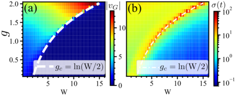
Figure 4: Single-particle dynamics; velocity and density fluctuation profiles. Panel (a) represents the sliding velocity $v_{G}=[x_{G}(t)-x_{G}(0)]/t$ [cf. Eq. (18)] indicated by a variation of plot colors indicated in the color bar at a given set of parameters $g$ and $W$; its distribution is shown in the $(W,g)$-plane. Evaluated at $t=t_{1}=20$. Panel (b) shows a similar plot for the density fluctuation, enumerated by the quantity: $\sigma(t)=\Delta x(t)-\Delta x(0)$, also evaluated at $t=t_{1}$; $\Delta x(t)$ is as given in Eq. (20). The same initial state as in Fig. 2 and Fig. 3. Average over $50$ samples with different $\theta_{0}$.

To further quantify features specific to the non-Hermitian wave packet dynamics, it may be natural to focus on

1. how fast the center of the gravity

   $$x_{G}(t)=\sum_{j}j|\psi_{j}(t)|^{2}$$ (18)

   of the wave packet moves, and also

2. to what extent the wave packet is spread around $x_{G}(t)$.

It turns out that $x_{G}(t)\simeq x_{G}(0)+v_{G}t$ so that 1. can be measured by the velocity $v_{G}$. In panel (a) of Fig. 4, the magnitude of $v_{G}$ is plotted (determined by evaluating $x_{G}(t)$ at $t=t_{1}$ ) as changing the set of parameters $(W,g)$, and is indicated by a variation of plot color. The plot shows that $v_{G}$ is finite in the extended phase $W<W_{c}$, while it practically vanishes in the localized phase $W>W_{c}$. The location of the phase boundary (6), or equivalently,

$$g=\log{W\over 2}$$ (19)

is indicated by a broken curve in the panel. On the side of the extended phase $W<W_{c}$, $v_{G}$ continues to take a relatively large value until quite close to the phase transition; at a fixed value of $g$, it rather tends to increase as $W$ increases until an abrupt fall at the phase transition.

Panel (b) shows a similar plot for the quantity: $\sigma(t)=\Delta x(t)-\Delta x(0)$ at some fixed time $t=t_{0}$, where $\Delta x(t)$ has been redefined as

$$\Delta x(t)=\sqrt{\sum_{j}(j-x_{G}(t))^{2}|\psi_{j}(t)|^{2}}.$$ (20)

The quantity $\sigma(t)=\Delta x(t)-\Delta x(0)$ is expected to measure 2. to what extent the density $\rho_{j}(t)$ is spread around $x_{G}(t)$ The plot shows that similarly to the behavior of $v_{G}$ in panel (a), the spread of the wave packet also shows a sharp distinction in the extended ($W<W_{c}$) and localized ($W>W_{c}$) phase. Here, in terms of $\Delta x(t)$, not only it takes a finite value on the side of the extended phase: $W<W_{c}$, but the appearance of a peak may be easily seen as $W$ is increased toward and close to the localization transition (19) at $g$ fixed. We interpret that this enhancement of $\sigma(t)$ slightly before the localization transition reflects the the cascade-like explosion of the wave packet seen in the density profile in Fig. 2, panel (c).

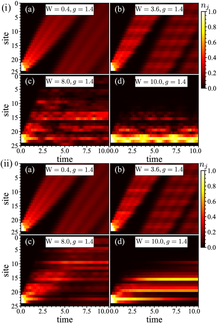
Figure 5: Multi-particle dynamics; evolution of the initial wave packet chosen to be in a domain wall form Eq. (22). The eight panels of Fig. 5 show the evolution of the particle density $n_{j}(t)$ as given in Eq. (24) at site $j$ and at time $t=t_{1}$; here $t_{1}$ is chosen as $t_{1}=2.2$, by a gradation of plot colors indicated in the color bar. The system size $L$ is set to $L=25$. Different panels (a-d) correspond to different values of disorder strength $W$; $W=0.4,3.6,8.0,10.0$, respectively, for panels (a-d). $g$ is fixed at $g=1.4$. $\theta_{0}=0$ (no disorder average). The four upper panel in the case (i) represent the non-interacting case: $V=0$, while those in (ii) represent an interacting case: $V=2$.

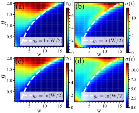
Figure 6: Multi-particle dynamics; velocity and density fluctuation profiles. Panels (a), (c) show distribution of the sliding velocity $v_{G}$, in the parameter space $(W,g)$, while panels (b), (d) represent a similar plot for $\sigma(t)=\Delta x(t)-\Delta x(0)$. $v_{G}$ and $\Delta x(t)$ are evaluated as in Eqs. (25) in the multi-particle case. Panels (a-b) represents the non-interacting case: $V=0$, panels (c-d) an interacting case: $V=2$. The same initial state as in Fig. 5; average over $50$ samples with different $\theta_{0}$.

II.2 Case of an interacting system

Here, we consider whether or not/how the presence of interaction may affect the above non-interacting picture. As a concrete model, we have employed the following bosonic version of the Hatano-Nelson $\times$ Aubry-André model with a nearest neighbor inter-particle interaction $V$:

$${\cal H} = -\sum_{j=0}^{L-1}\Big{(}\Gamma_{L}b_{j}^{\dagger}b_{j+1}+\Gamma_{R}b_{j+1}^{\dagger}b_{j}\Big{)}$$ (21)

$$+ \sum_{j=0}^{L-1}\Big{(}V\hat{n}_{j}\hat{n}_{j+1}+W_{j}\hat{n}_{j}\Big{)},$$

where $b_{j}^{\dagger}$ ($b_{j}$) creates (annihilates) a particle at site $j$, while $\hat{n}_{j}=b_{j}^{\dagger}b_{j}$ counts the number $n_{j}$ of such particles found at site $j$. Following Refs. Hamazaki et al., 2019, Zhai et al., 2020, we assume that our particles are hard-core bosons: $n_{j}=0,1$.

Fig. 5 shows the examples of multi-particle dynamics in this system when the initial state is chosen to be the following domain wall state

$$|\Psi(t=0)\rangle=|00\cdots 011\cdots 1\rangle,$$ (22)

i.e., the last $N_{b}$ sites are occupied in the local basis; $N_{b}$ represents the number of particles (bosons) in the system; in this numerical shown in Fig. 5 it is chosen as $N_{b}=3$. At time $t$, the initial state (22) evolves as

$$|\Psi(t)\rangle=\sum_{\mu}c_{\mu}e^{-iE_{\mu}t}|\mu\rangle,$$ (23)

where $|\mu\rangle$ is the eigenstate of the Hamiltonian Eq. (21);

$E_{\mu}$ is the corresponding eigenenergy: ${\cal H}|\mu\rangle=E_{\mu}|\mu\rangle$, while $c_{\mu}=\langle\langle\mu|\Psi(t=0)\rangle$. Here, $\langle\langle\mu|$ represents the left eigenstate corresponding to the eigenenergy $E_{\mu}$: $\langle\langle\mu|{\cal H}=E_{\mu}\langle\langle\mu|$ and not $|\mu\rangle^{\dagger}$; $\langle\langle\mu|\neq|\mu\rangle^{\dagger}$. We make sure that the left and right eigenstates satisfy the biorthogonal condition, i.e., $\langle\langle\mu|\nu\rangle=\delta_{\mu,\nu}$. These are analogous to the single-particle case. Also, as the single-particle eigenenergy $\epsilon_{n}$ is complex in general, so is the many-body eigenenergy $E_{\mu}$. As a result, the time-evolved wave packet $|\Psi(t)\rangle$ as given in Eq. (23) tends to grow exponentially. To avoid this computational difficulty, we rescale (renormalize) $|\Psi(t)\rangle$ in the same way as in Eq. (9) at every interval $\Delta t\simeq 10^{-4}-10^{-1}$ in the actual computation. The eight panels of Fig. 5 show the evolution of the particle density

$$n_{j}(t)=\langle\Psi(t)|\hat{n}_{j}|\Psi(t)\rangle$$ (24)

at site $j$ at time $t$ by a color variation; the higher is the density, the brighter the color is. The system size $L$ is set to $L=25$. The four panels in the upper case (i) represents the non-interacting case: $V=0$, while those in the lower case (ii) represents an interacting case: $V=2$. In these panels one can still see the tendency observed in the single-particle dynamics; e.g., the cascade-like feature in wave packet spreading can be seen in panels (c) [both in (i) and (ii)].

Figs. 6 represent the distribution of $v_{G}$ and $\sigma(t)=\Delta x(t)-\Delta x(0)$ in the parameter space: $(W,g)$; the two figures correspond, respectively, to the cases of $V=0$ and $V=2$. $v_{G}$ and $\sigma(t)$ are calculated similarly in the single-particle case; i.e., via,

$$x_{G}(t) = \sum_{j}jn_{j}(t)\simeq x_{G}(0)+v_{G}t,$$

$$\Delta x(t) = \sqrt{\sum_{j}(j-x_{G}(t))^{2}n_{j}(t)/\sum_{j}n_{j}(t)}.$$ (25)

In both of the figures the two quantities $v_{G}$ and $\sigma(t)$, both take a finite value on the side of the extended phase: $W<W_{c}$, while they vanish on the localized side: $W>W_{c}$. In $\sigma(t)$ [panels (b)], one can also clearly see an enhancement before the localization transition. Thus, the specific and unusual features in wave packet spreading characteristic to non-Hermitian systems found in the single-particle dynamics are, though somewhat masked by the inter-particle interaction $V$, essentially maintained in the multi-particle dynamics.

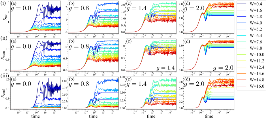
Figure 7: Entanglement dynamics; non-interacting case ($V=0$). Three panels (i-a), (ii-a), (iii-a) in the first column represent the Hermitian case $g=0$, while other panels represent non-Hermitian cases $g\neq 0$; $g=0.8$ for panels (i-b), (ii-b), (iii-b) in the second column (in this case, $W_{c}=2\Gamma_{L}=2\Gamma_{0}e^{g}\simeq 4.5$), $g=1.4$ for panels (i-c), (ii-c), (ii-d) in the third column ($W_{c}\simeq 8.1$), $g=2$ for panels (i-d), (ii-d), (iii-d) in the fourth column ($W_{c}\simeq 14.8$). Four panels (i-a), (i-b), (i-c), (i-d) in the first raw represent the evolution of the total entanglement entropy $S_{\rm tot}(t)$, while panels (ii-a), (ii-b), (ii-c), (ii-d) in the second raw, and panels (iii-a), (iii-b), (iii-c), (iii-d) in the third raw represent, respectively, the number and configuration entropies, $S_{\rm num}(t)$ and $S_{\rm conf}(t)$. The system size is $L=12$. Density-wave type initial state (26); average over $50$ samples with different $\theta_{0}$.

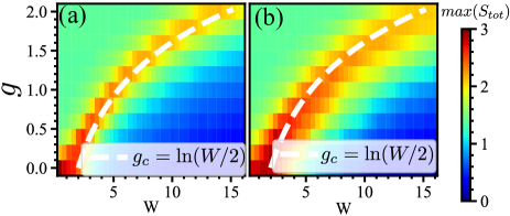
Figure 8: Distribution of the maximal entanglement entropy, Max $S_{\rm tot}(t)$ in the $(W,g)$ parameter space. The maximal value of $S_{\rm tot}(t)$ in the time evolution is plotted (a) non-interacting case: $V=0$ (the corresponding time evolution is plotted in Fig. 7), (b) interacting case: $V=2$ (id. in Fig. 7). The location of the delocalization-localization transition in the non-interacting case: $g=\log W/2$ [as given in Eq. (19)] is indicated by a broken curve (in white) as a guide for the eyes. Based on the same data as in Figs. 7, 10.

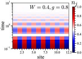
Figure 9: Damped oscillatory behavior in the density profile $n_{j}(t)$. Evolution of the particle density $n_{j}(t)=\langle\Psi(t)|\hat{n}_{j}|\Psi(t)\rangle$ as given in Eq. (24) is plotted for the density-wave type initial state Eq. (26). The magnitude of $n_{j}(t)$ at site $j$ (abscissa) and at time $t$ (ordinate) is expressed by a variation of plot color indicated in the color bar. g=0.8,W=0.4$,\theta_{0}=0$, $L=12$; no disorder averaging.

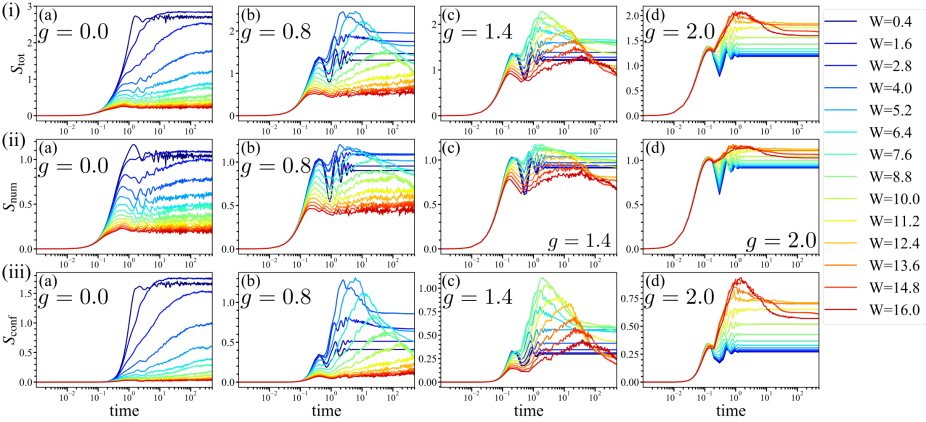
Figure 10: Entanglement dynamics; interacting case ($V=2$). Similarly to the case of Fig. 7, three panels (i-a), (ii-a), (iii-a) in the first column represent the Hermitian case $g=0$, while other panels represent non-Hermitian cases $g\neq 0$; $g=0.8$ for panels (i-b), (ii-b), (iii-b) in the second column, $g=1.4$ for panels (i-c), (ii-c), (iii-c) in the third column, $g=2$ for panels (i-d), (ii-d), (iii-d) in the fourth column. The precise value of $W_{c}$ is unknown in the interacting case ($V\neq 0$), but will be not far from (slightly larger than) the non-interacting values given in the main text and in the caption of Fig. 7. $L=12$. Other conditions are the same as in Fig. 7; average over $50$ samples with different $\theta_{0}$.

III The entanglement dynamics

The entanglement entropy measures how quasiparticles spread and entangle a quantum states in the systemCalabrese and Cardy (2005); Chiara et al. (2006); Alba and Calabrese (2018). In a non-interacting system, this signifies how a wave function spreads in the system; the entanglement entropy increases as the wave function spreads in the system. In dynamics, this occurs in the process of wave packet spreading. The initial growth of the number entropy $S_{\rm num}(t)$ in the quench dynamics is essentially due to this effect. In Hermitian systems with reciprocal hopping $\Gamma$ an initially localized wave packet spreads symmetrically in the two directions in the clean limit and after a duration $t$ the wave function becomes extended to a region of width $\Delta x\sim 2v_{f}t$, where $v_{f}$ is the velocity of the wave front: $v_{f}\simeq J$; Longhi (2021) the entanglement entropy also increases as $S(t)\propto\Delta x\sim 2v_{f}t$. In interacting systems, the same argument applies to quasiparticles, with being the notion of $v_{f}$ replaced with the Lieb-Robinson velocity.Lieb and Robinson (1972) The interaction also makes the superposition of eigenstates “nontrivial” in the time evolution of a wave packet, leading to generation of entanglement (entropy). In the presence of disorder $W$, as its strength is increased, wave packet spreading tends to be suppressed; $v_{f}$ tends to be suppressed and at some critical value $W=W_{c}$, $v_{f}$ vanishes. When $W>W_{c}$, the wave function is localized and wave packet spreading is essentially suppressed. As for the behavior of $S_{\rm tot}(t)$, it experiences a rapid growth in the time scale wave packet spreading prevails in the system in the extended phase, while such a growth is much suppressed in the localized phase [see Fig. 7, panel (i-a)]. Serbyn et al. (2013)

Having in mind how wave packet spreads in non-Hermitian systems with non-reciprocal hopping, we proceed to the analysis of how the entanglement entropy $S_{\rm tot}(t)$ evolves in time in such systems. We employ the same many-body Hamiltonian (21) as in the analysis of wave packet spreading, while the initial (many-body) wave packet is chosen to be the following density wave form (or Néel form in the pseudo-spin language Panda and Banerjee (2020)):

$$|\Psi(t=0)\rangle=|101010\cdots\rangle,$$ (26)

where on the right hand side of the equation we have employed the computational basis $|\nu\rangle=|n_{1}n_{2}\cdots n_{L}\rangle$; $n_{j}=0,1$ represents occupation of the $j$th site.

The entanglement entropy $S(t)$ can be found by tracing out “a half” of the system; i.e., we divide the system of length $L$ into two subsystems $A$ and $B$ of length $L/2$, where a site $j$ in $A$ satisfies $j\in j_{A}=\{1,2,\cdots,L/2\}$, while $j$ in $B$ satisfies $j\in j_{B}=\{L/2+1,L/2+2,\cdots,L\}$. We then, by tracing out the subsystem $B$, calculate the entanglement entropy $S_{A}(t)$ for the subsystem $A$. To concretize this procedure, we employ the density matrix,

$$\Omega(t)=|\Psi(t)\rangle\langle\Psi(t)|,$$ (27)

and perform its partial trace:

$$\Omega_{A}(t)=\rm{Tr}_{B}\ \Omega(t),$$ (28)

where in Eq. (27) $|\Psi(t)\rangle$ represents a many-body state at time $t$ evolved from Eq. (26). Then, we introduce the entanglement entropy:

$$S_{A}(t)=-{\rm Tr}\ \Omega_{A}(t)\log\Omega_{A}(t),$$ (29)

which is related to the eigenvalues $\lambda_{\alpha}(t)$ of the reduced density matrix $\Omega_{A}(t)$ as

$$S_{A}(t)=-\sum_{\alpha}\lambda_{\alpha}(t)\log\lambda_{\alpha}(t).$$ (30)

III.1 Two types of contributions to the entanglement entropy: number and configuration entropies

If the number of particles in subsystem $A$, i.e.,

$$N_{A}=\sum_{j\in j_{A}}n_{j}$$ (31)

is a good quantum number in the subsystem; i.e., if

$$[\Omega_{A},N_{A}]=0$$ (32)

holds, the contributions to the entanglement entropy $S_{\rm tot}(t)=S_{A}(t)$ can be divided into two parts; they are the number and configuration entropies: Lukin et al. (2019)

$$S_{\rm tot}(t)=S_{\rm num}(t)+S_{\rm conf}(t),$$ (33)

where

$$S_{\rm num} = -\sum_{N_{A}}p_{N_{A}}\log\ p_{N_{A}},$$ (34)

$$S_{\rm conf} = -\sum_{N_{A}}\sum_{\alpha}p_{N_{A}}\tilde{\lambda}^{(N_{A})}_{\alpha}\log\ \tilde{\lambda}^{(N_{A})}_{\alpha}.$$ (35)

To find the formulas (34), (35), let us first notice that the reduced density matrix $\Omega_{A}$ is block diagonal since $N_{A}$ and $\Omega_{A}$ are simultaneously diagonalizable [cf. Eq. (32)]; i.e.,

$$\Omega_{A}=\Omega_{N_{1}}\oplus\Omega_{N_{2}}\oplus\Omega_{N_{3}}\oplus\cdots$$ (36)

where $\Omega_{N_{A}}$’s are diagonal blocks of $\Omega_{A}$ in which the number of particles in the subsystem A is restricted to $N_{A}$. Correspondingly, the eigenvalues $\lambda_{\alpha}$ of the full reduced density matrix $\Omega_{A}$ are grouped into those of $\Omega_{N_{A}}$’s. Let us denote an eigenvalue of $\Omega_{N_{A}}$ as $\lambda^{(N_{A})}_{\alpha}$. Using $\lambda^{(N_{A})}_{\alpha}$, we define $p_{N_{A}}$, then rescale the eigenvalues in this subspace as

$$p_{N_{A}} = \sum_{\alpha}\lambda^{(N_{A})}_{\alpha},$$ (37)

$$\tilde{\lambda}^{(N_{A})}_{\alpha} = {1\over p_{N_{A}}}\lambda^{(N_{A})}_{\alpha}.$$ (38)

Note that unlike in Eq. (30) the summation over $\alpha$ in Eqs. (35) and (37) does not run over all the eigenstates of the full reduced density matrix $\Omega_{A}$ but only in the subspace with fixed $N_{A}$.

The number entropy $S_{\rm num}$ quantifies the fluctuation of the number of particles in the subsystem A. Particle transport across the subsystems generates this type of entropy; i.e., $S_{\rm num}$ is controlled by a local process. Recent numerical studies have focused on whether or not $S_{\rm num}$ saturates in the MBL phase.Kiefer-Emmanouilidis et al. (2020); Luitz and Lev (2020); Yao et al. (2021) If $S_{\rm num}$ is not saturated in the putative MBL phase, it implies that the particles are still transporting and in this sense localization is not perfect. The configuration entropy $S_{\rm conf}$ comes from non-local correlations in the many-body state, while the distinction between many-body and single-body localizations is also presumed to be the presence or absence of non-local correlations. Thus, the configuration entropy has the potentiality to probe such features that are specific to MBL, and reveal its unique mechanism of localization; Chen and Wang (2021); Orito et al. (2021a); Sierant et al. (2019) e.g., in Ref. Sierant et al., 2019, non-trivial entanglement growth due to cavity-mediated long-range interactions is evaluated via the use of configuration entropy.

III.2 The entanglement entropy in the non-interacting limit: wave packet spreading vs. entanglement entropy

Fig. 7 shows time evolution of the entanglement entropy for the initial state (26) in non-interacting systems with a variable strength of non-Hermiticity $g$. Panels (i-a), (ii-a), (iii-a) represent the Hermitian case $g=0$; the three panels represent, respectively, (i-a) $S_{\rm tot}(t)$, (ii-a) $S_{\rm num}(t)$, (iii-a) $S_{\rm conf}(t)$. The peculiarity of the Hermitian limit is that having symmetric amplitudes in the two hopping directions, the system is in a subtle equilibrium in which the interference of many plane-wave eigenstates [cf. Eq. (10)] leads to particle spreading in the delocalized regime. Here, in terms of the entanglement entropies, they show a rapid initial growth and a high saturated value in such weak $W$ regime, while as $W$ is further increased to the localized regime: the entropies tend to be strongly suppressed. In panel (ii-a) we focus on the behavior of the number entropy $S_{\rm num}(t)$. In the regime of weak disorder: $W=0.4,1.6$, $S_{\rm num}(t)$ first rapidly grows, and then saturates practically to the same value. To be precise, as $W$ increases, the quick initial growth of $S_{\rm num}(t)$ tends to slow down toward the saturation at the end of the initial growth. In any case, in the delocalized regime: particles spread and after a sufficiently long time (although this time lengthens as $W$ increases) the system reaches the equilibrium. $S_{\rm conf}(t)$ also grows in the delocalized regime, but the growth occurs with a slight delay with respect to that of $S_{\rm num}(t)$ [see Fig. 7 (iii-a)]. As $W$ exceeds the critical value $W_{c}=2$, both the number and configuration entropies decrease, but remain finite. This is because even in the localized phase, there is a finite localization length $\xi$,Kiefer-Emmanouilidis et al. (2020) and especially if $W$ is not too large and the system is not far from the transition, this effect is non-negligible (see Appendix D).

We have seen in Sec. II-A that addition of non-Hermiticity $g\neq 0$ has a more drastic impact on the wave packet dynamics, breaking the subtle equilibrium on the direction of particle motion, and consequently, the reality of the eigenvalues. In the presence of $g\neq 0$ the wave packet ceases to spread, but starts to slide. We have also seen in the previous section that as $W$ increases, this sliding velocity often increases, and when $W$ is further increased and approaches the critical value $W_{c}$, the wave packet also starts to “spread”, showing a cascade-like feature as in the hermitian case at weak $W$. Under this circumstance close to the localization transition a particle may be rather undecided about which way to go in spite of the finite non-reciprocal hopping $g\neq 0$, and a situation somewhat similar to the Hermitian case seems to be realized. In the Hermitian case, we have seen that the entanglement entropies diminish as $W$ increases, while in panels (i-b)-(i-d) of Fig. 7, i.e., as $g$ is increased, this tendency starts to be uncertain and finally the tendency is just reversed. This result indicates that disorder generates entanglement entropy and showing a maximum at some finite $W=\tilde{W}_{c}$, then they turn to decrease. We argue that this maximum of the entanglement entropies is related to the delocalization-localization transition. In Fig. 8 (a), the maximal value Max $S_{\rm tot}(t)$ of the entanglement entropy is plotted in the ($W,g$)-plane. The distribution of Max $S_{\rm tot}(t)$ resembles very much that of $\sigma(t)=\Delta x(t)-\Delta x(0)$, in Fig. 4 (b), showing a peak close to the boarder Eq. (19) to the localized phase (if seen from the weak $W$ (delocalized) side); i.e., “the maximum of Max $S_{\rm tot}(t)$” coincides with the regime where a cascade-like expansion of wave packet occurs in the density dynamics. In other words, the maximum of Max $S_{\rm tot}(t)$ occurs close to the delocalization-localization transition: $\tilde{W}_{c}=W_{c}$. The unusual behavior of entanglement entropies in the non-Hermitian non-reciprocal system is thus revealed to be directly related to a very specific way how wave packet spreads (or rather, does not occur) in this system.

Finally, let us comment on the number and configuration entropies. Figs. 7(ii-b)-(ii-d) show the time evolution of number entropy, in the delocalized phase, the number entropy first show a rapid initial growth with a speed almost independent of $W$, then they show a second growth which looks more like a damped oscillation. The mechanism of damped oscillation come from the convergence to a single eigenstate $|\mu_{0}\rangle$ with the maximal imaginary part of eigenenergy $E_{\mu_{0}}$, this also reflects the time evolution of density profile as shown in Fig. 9. Convergence to a single eigenstate with the maximal imaginary part of eigenenergy also leads to suppression of the configuration entropy as shown in Figs. 7(iii-b)-(iii-d). The convergence to a single destined eigenstate $|\mu_{0}\rangle$ implies the loss of superposition; the configuration entropy is significantly reduced in this regime of $W\simeq 0$. The destined eigenstate is delocalized so that after certain time the initial density wave pattern Eq. (22) is almost washed out; see Fig. 9, while the number and configuration entropies show a damped oscillation before they converge to a finial value. Beyond a critical disorder strength $W_{c}$, the number, and configuration entropy look rather fluctuating (fast and randomly) as in the Hermitian case.

III.3 Case of $V\neq 0$ and $g\neq 0$ as well: the non-monotonic behavior

We switch on the interaction: $V\neq 0$. Similarly to the non-interacting case, panels (i-a), (ii-a), (iii-a) of Fig. 10 show the evolution of the entanglement entropy in the Hermitian limit: $g=0$; the three panels represent, respectively, the cases of (i-a) $S_{\rm tot}(t)$, (ii-a) $S_{\rm num}(t)$, (iii-a) $S_{\rm conf}(t)$. Comparing these panels with the corresponding panels in the non-interacting case [Fig. 7 (i-a), (ii-a), (iii-a)], one can observe that the total entanglement entropy $S_{\rm tot}(t)$ [panel (i-a)] shows a quick initial growth until around 2-5$\times 10^{1}$, then the growth slows down and smoothly crosses over to a linear regime (in the logarithmic time scale). Comparing these behaviors in panel (i-a) with the ones in panel (ii-a) one notices that the quick initial growth comes from the number entropy $S_{\rm num}(t)$, while the second slow growth forming a linear regime stems from the configuration entropy $S_{\rm conf}(t)$ in panel (iii-a).

As the non-Hermiticity $g$ is also switched on; see remaining panels of Fig. 10, the entanglement dynamics changes its face as in the non-interacting case; cf. corresponding panels in Fig. 7, but here, in the interacting case a feature not existing in the non-interacting case also come into play; after the second slow growth the entanglement entropies start to decay, exhibiting a characteristic non-monotonic behavior. The non-monotonic behavior appears in the intermediate regime of $W$, but it is unclear whether it stems from the delocalized phase or localized phase. We employ the saturated value of the entropies to which are expected to be maximal at $W_{c}$ close to the delocalization-localization transition as in the non-interacting case. In Fig. 8, panel (b), the maximal value Max $S_{\rm tot}(t)$ in the time evolution is plotted in the parameter space $(W,g)$, showing a broader maximum compared with the non-interacting case [panel (a)], while the location of the peak is slightly shifted to the side of larger $W$ from the non-interacting value (indicated by a white broken curve). The location of the phase boundary estimated from the peak of Max $S_{\rm tot}(t)$ in Fig. 8 (b) is consistent with an earlier numerical result: $W_{c}\simeq 6-7$ at $g=0.5$ in Ref. Zhai et al., 2020. Comparing Fig. 8 with Fig. 10, one can observe that the non-monotonic behavior appears in the regime of $W$ corresponding to the critical-localized regime.

The mechanism of the non-monotonic evolution, which is a consequence of the competition between (i) dephasing and (ii) convergence (or a gradual “collapse”) of the superposition [Eq. (23)] into a single (non-equilibrium steady) state Panda and Banerjee (2020) $|\mu_{0}\rangle$ with a maximal imaginary part of the eigenenergy $E_{\mu_{0}}$. In the absence of (ii), (i) leads to a slow but unbounded (in the MBL phase, typically logarithmic)Serbyn et al. (2013) growth of the configuration entropy, while for (ii) to be operational the eigenenergy must have a finite imaginary part Im $E_{\mu}$. Panels (iii-b)-(iii-d) of Fig. 10 show the evolution of configuration entropy at different set of parameters. They show that in the localized regime the non-monotonic behavior of the entanglement entropy (panels (i-b)-(i-d) of Fig. 10) stems mainly from the contribution of configuration entropy. Note that the dephasing enhanaces, while the convergence suppresses the configuration entropy. In the localized regime these two effects compete, leading to a non-monotonic entanglement evolution, while in the delocalized phase, convergence dominates dephasing; therefore, no non-monotonic behavior appears. In the non-interacting case: $V=0$, the localization transition is believed to coincide with the real-complex transition,Hatano and Nelson (1996, 1997, 1998) while in the interacting case: $V\neq 0$, whether the superposition (23) converges (collapses) to a non-equilibrium steady state on the MBL side is a more subtle issue.

Finally, we discuss the behavior of number entropy. In the delocalized phase, the damped oscillatory behavior mentioned earlier is more conspicuous. As the $W$ is increased, the damped oscillation disappears and replaced with a non-monotonic behavior with a broader maximum. On top of the non-monotonic behavior one can also recognize a fast oscillatory component. Such an oscillatory component is also conspicuous in the non-interacting case, especially in the localized regime. In the non-interacting limit the disappearance of damped oscillation coincides with the localization transition. Here, we have shown that this is also the case in an interacting system.

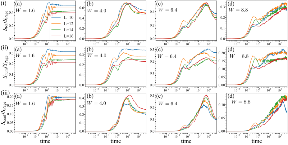
Figure 11: Time evolution of the entanglement entropies; the first raw [panels (i-a)-(i-d)]: $S_{\rm tot}(t)$, the second raw [panels(ii-a)-(ii-d)]: $S_{\rm num}(t)$, and the third raw [panels (iii-a)-(iii-d)]: $S_{\rm conf}(t)$. The system is both non-Hermitian: $g=0.6\neq 0$, and interacting: $V=2$. Each column represents data at the same value of $W$, which evolves from left to right as $W=1.6,4.0,6.4,8.8$. Curves plotted in different colors correspond to different system size, as indicated in the inset of panel (i-a). Density-wave type initial state (26); average over $50$ samples with different $\theta_{0}$.

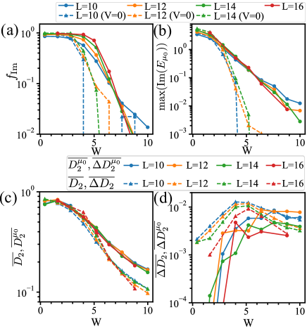
Figure 12: Size dependence of (a) the fraction of imaginary eigenvalues: $f_{\rm Im}$ [cf. Eq. (40)], (b) Max (Im $E_{\mu_{0}}$), (c) the multifractal dimension $D_{2}$, and (d) its fluctuation: $\Delta D_{2}$. Data taken for an interacting case: $V=2$ (connected by solid lines) is compared with the non-interacting case: $V=0$ (connected by broken lines). Different colors correspond to different system size: $L=10,12,14,16$. $\theta_{0}$-averaged (50 samples).

IV Effects of finite size and non-equilibrium steady state

Let us comment on the effects of system size. In the three raws of panels in Fig. 11 we compare the evolution of the entanglement entropies: (i-a)-(i-d) $S_{\rm tot}(t)$, (ii-a)-(ii-d) $S_{\rm num}(t)$, and (iii-a)-(iii-d) $S_{\rm conf}(t)$ for systems of different system size $L$. Note that the entropies are normalized by the “Page value”,Page (1993) given in the case of $N_{A}=N_{B}=L/2$ as

$$S_{\rm Page}={L\over 2}\log 2-{1\over 2}.$$ (39)

Note that $S_{\rm Page}$ is proportional to the size $L$ of the system; if plotted curves; i.e. the entanglement entropies calculated at different system size $L$ are size independent, then it means that that entropy obeys the volume law in the range of parameters in question. In the Hermitian case the magnitude of $S_{\rm tot}(t)$ is size independentLuitz et al. (2016); Lee et al. (2017) at the stage of initial quick growth (area law), while its saturated value after duration of a long enough time is size-dependent ($\propto L$), obeying a volume lawSerbyn et al. (2013); Bardarson et al. (2012). In the first raw of Fig. 11 [panels (i-a)-(i-d); different panels correspond to different strength of disorder $W$. $g$ is fixed at $g=0.6$.] the total entanglement entropy $S_{\rm num}(t)/S_{\rm Page}$ is plotted at different system size $L$. The magnitude of $S_{\rm tot}(t)/S_{\rm Page}$ is clearly decreasing with the increase of $L$ in panel (i-a), implying an area-law behavior, while in panel (i-b)-(i-c) [$W=4.0$ in panel (i-b), $W=6.4$ in panel (i-c); both values of $W$ are assumed to be not far from $W_{c}^{(V=2)}$] it becomes size dependent at its maximum ($t\simeq 3-7\times 10^{1}$), suggesting a volume-law behavior. As $W$ is further increased [panel (i-d): $W=8.8$], the second growth of $S_{\rm num}(t)$ (a linear growth region in the logarithmic time scale) lasts longer, and the maximum of $S_{\rm num}(t)$ is not really achieved in the time scale shown in the panel.

Comparing panels (i-a), (ii-a), (iii-a), one can see that the area-law size dependence of $S_{\rm tot}$ stems from that of $S_{\rm num}$, while comparing panels (i-c), (ii-c), (iii-c), one can see that the volume-law behavior of Max $S_{\rm tot}$ results from an interplay of the number and configuration entropies. The insensitivity of Max $S_{\rm tot}$ to the system size $L$ suggests that the non-monotonic evolution of the entanglement entropy specific to the non-Hermitian many-body system will also occur in cases of larger system size $L$.

For further clarifying this point we have plotted, in panel (a) of Fig. (12), the ratio

$$f_{\rm Im}=D_{\rm Im}/D,$$ (40)

where $D_{\rm Im}$ is the number of eigenenergies with a nonzero ($|{\rm Im}E_{\mu}|>10^{-13}$) imaginary part Im $E_{\mu}$, while $D$ is the dimension of the Hilbert space; i.e., the total number of eigenenergies. The existence of nonzero Im $E_{\mu}$ leads to suppression of the superposition (23), leading also to the suppression of the entanglement entropies. The delocalized eigenstates are susceptible of the non-reciprocity $g$ of hopping, generating a finite imaginary part in the eigenenergy. Thus, the quantity $f_{\rm Im}$ measures the fraction of delocalized eigenstates in the total ensemble of eigenstates. Panel (a) of Fig. 12 shows the evolution of the fraction $f_{\rm Im}$ with the increase of $W$ for systems of different size $L$. As $W$ is increased, $f_{\rm IM}$ first very gradually, then quickly decreases; this tendency is more accentuated in systems of larger size $L$. Also, the curves corresponding to different system size $L$ cross practically at the same point [at least in the interacting case: $V=2$, cases of solid curves in panel (a)] at a value of $W=W_{c}\simeq 7$. In a system of size $L$ sufficiently large the curve $f_{\rm Im}(W)$ tends to become a sharply edged function: $f_{\rm Im}(W)\simeq 1$ for $W<W_{c}$, while $f_{\rm Im}(W)\rightarrow 0$ for $W>W_{c}$; i.e., in this case practically all the eigenstate, including highly excited states, they altogether experience a complex-to-real transition of eigenvalues; they all, at least, most of them turn real at $W=W_{c}$.

In panel (b) of Fig. 12 we compare the (ensemble-averaged) maximal value of Im $E_{\mu}$ in the cases of $V=0$ and $V\neq 0$. As expected, in the non-interacting case: $V=0$, the magnitude of Max(Im $E_{\mu}$) experiences an abrupt fall at the crossing (size-independent) point: $W=W_{c}\simeq 3-4$; on the two sides of this transition point the behavior of Max(Im $E_{\mu}$) shows a clear change that tends to magnify as the system size $L$ increases. In particular, in the localized phase ($W>W_{c}$) the magnitude of Im $E_{\mu}$ tends to vanish as $L$ increases. In the interacting case ($V\neq 0$) [Fig. 12 (b) solid curves], on the other hand, the ensemble-average of Max(Im $E_{\mu}$) does not show an abrupt fall; instead, it gradually decays over a broad range of $W$. It shows no clear signature, in the ETH-MBL crossover/transition regime: $W\simeq W_{c}$. Besides, it shows no dependence on the system size $L$, either. Based on these observations, we presume that generically, Im $E_{\mu}$ remains finite even on the MBL side: $W>W_{c}$; i.e., the superposition (23) converges to a non-equilibrium steady state $|\mu\rangle=|\mu_{0}\rangle$ with a maximal Im $E_{\mu}$ even though it may take a longer time until the collapse than in the ETH phase. One may ask what the nature of this steady state $|\mu_{0}\rangle$ is. Is it really a localized state? This question arises, of course, since one usually associates the imaginary part of $E_{\mu}$ with an extended state. To clarify this point we have estimated the multi-fractal dimension

$$D_{2}^{\mu}=-{\log(\sum_{\nu=1}^{D}|c_{\nu}^{\mu}|^{4})\over\log(D)},$$ (41)

encoding the (de)localized nature of the eigenstate $|\mu\rangle$; $D_{2}^{\mu}=1$ ($=0$) corresponds to a fully delocalized (localized) eigenstate. $c_{\nu}^{\mu}$’s are the amplitudes of computational basis $|\nu\rangle=|n_{1}n_{2}\cdots n_{L}\rangle$ of $\mu$th eigenstate and $D$ is the dimension of the many-body Hilbert space. In panel (c) of Fig. 12, disorder averaged $\overline{D_{2}^{\mu_{0}}}$ (represented by solid lines) compared with disorder and all eigenstates averaged $\overline{D_{2}}$ (represented by broken lines).

The plots show that in the deep MBL regime, the eigenstates $|\mu_{0}\rangle$ show a localized tendency, even though its eigenenergy E has a finite imaginary part; to be precise, the state $|\mu_{0}\rangle$ is less localized than other eigenstates. Panel (d) of Fig. 12 shows the variance $\overline{\Delta D_{2}}$ of the multi-fractal dimension as a function of $W$, which suggests a qualitatively different behavior in the ETH-MBL crossover regime for $\overline{\Delta D_{2}}$ and $\overline{\Delta D_{2}^{\mu_{0}}}$. To summarize, the superposition (23) indeed converges (collapses) to a non-equilibrium steady state $|\mu_{0}\rangle$ even in the deep MBL phase, while the destined state $|\mu_{0}\rangle$ shows spatially a localized signature.

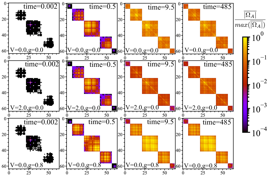
Figure 13: Evolution of the reduced density matrix in the wave-packet dynamics. (i) the first raw: Hermitian limit ($g=0$), non-interacting case ($V=0$); result of simple wave packet spreading. (ii) the second raw: Hermitian limit ($g=0$), interacting case ($V\neq 0$); both wave packet spreading and dephasing occur in the dynamics. (iii) the third raw: Non-Hermitian case ($g\neq 0$), non-interacting ($V=0$). The same initial state as in Fig. 7; $\theta_{0}$-averaged (50 samples).

V Mapping the reduced density matrix $\Omega_{A}(t)$

Let us finally visualize how different stages in the time evolution of the entanglement entropy can be understood from the viewpoint of the behavior of the reduced density matrix $\Omega_{A}(t)$. In the twelve panels Fig. 13 we have plotted the elements of $\Omega_{A}(t)$ at different times in order to visualize its time evolution. We will see that there are 4-5 characteristic stages in the evolution of $\Omega_{A}(t)$.

In the first raw of Fig. 13, we start with the Hermitian case ($g=0$) with no interaction ($V=0$). At $t=0$ the initial state $|\Psi(t)\rangle$ is chosen to be a simple product state so that the reduced density matrix $\Omega(t=0)$ has a single finite element ($=1$) in one of the diagonals. As time passes by, the region of a finite matrix element (represented by bright spots in the panels) spreads, but for a while; e.g., case of the first panel from the left ($t=0.002$), most of the amplitudes stay in the same diagonal block in some $\Omega_{N_{A}}$ ($N_{A}=N_{1},N_{2},\cdots$) [cf. Eq. (36)] From the start of the quench dynamics, the system is susceptible to the process of wave packet spreading, but as far as $N_{A}$ is kept unchanged, such a dynamics does not lead to an immediate increase of the number entropy. After some time; e.g., case of the second panel ($t=0.5$), bright spots start to appear in the neighboring blocks, and finally; e.g., cases of the third and fourth panels ($t=9.5,485$), they become distributed almost equally in all the blocks. It is expected that the number entropy experiences a rapid growth in this period and becomes saturated afterwards.

Let us switch on the interaction ($V\neq 0$)); Fig. 13, the second raw. In the first two panels, the evolution of $\Omega_{A}(t)$ looks similar to the non-interacting case; i.e., as time passes by, bright spots tend to spread over all different blocks, meanwhile the number entropy tends to be saturated. In the third and fourth panels, the bright spots look distributed equally in all the blocks as in the non-interacting case, but here inside each block $\Omega_{N_{A}}$ they converge on the diagonals. This is due to dephasing.Serbyn et al. (2013) Due to the interaction $V\neq 0$, off-diagonal matrix elements tend to acquire a random phase, which on average tends to vanish after some time. Dephasing leads to increase of the configuration entropy $S_{\rm conf}(t)$; thus, in the present case after the number entropy is saturated, the total entanglement entropy $S_{\rm tot}(t)$ continues to increase with no systematic bound excepting the one due to the size of the system.

In the non-Hermitian case: $g\neq 0$ and also at $V=0$; Fig. 13, the third raw, the overall behavior of the evolution of the reduced density matrix $\Omega_{A}(t)$ resembles the Hermitian case in the first raw except that here inside each block $\Omega_{N_{A}}$ the pattern of the matrix elements looks very regular, while the patten looks random in the Hermitian case ($g=0$). The reason will be the following: here, in the regime of weak $W$, the eigenenergy $E$ is typically complex, so that in the time evolution (23) of a (many-body) wave packet $|\Psi(t)\rangle$, a single eigenstate $|\mu\rangle=|\mu_{0}\rangle$ with a maximal imaginary part ${\rm Im}\ E_{\mu}$ tends to predominate in the superposition (23). We have already seen this tendency in the evolution of the entanglement entropy $S_{\rm tot}(t)$ (cf. Fig. 7); in the regime of weak $W$, $S_{\rm tot}(t)$ quickly converges to a fixed value and shows practically no fluctuation.

VI Concluding remarks

In this paper, we have elucidated the physics of non-Hermitian ETH-MBL transition from the viewpoint of unusual (or rather, disappearance of) wave packet spreading and through analyses of the time evolution of entanglement entropies. In the first half of the manuscript, we have highlighted the nature of the unusual wave packet spreading in a non-Hermitian system with non-reciprocal hopping (Hatano-Nelson model) [Eqs. (1), (21)]. Disorder has been modeled by a quasi-periodic potential (Aubry-Andre model) [Eq. (2)]. In a Hermitian system wave packet spreading is gradually suppressed by disorder, while here in a non-Hermitian system it simply does not occur; even in the clean limit, at least in the Hermitian way. The wave packet rather slides and not spread. Weak disorder exerts little effect on this behavior, while as it becomes strong enough to practically disable the non-reciprocity, the characteristic sliding behavior tends to be replaced with a cascade-like wave packet spreading analogous to the Hermitian case. We have clearly demonstrated the mechanism [see Eq. (17), and related arguments] why the wave packet slides and not spread in our system, and how such a behavior tends to be destroyed by the quasi-periodic potential (cf. Fig. 3). In the non-Hermitian case the fundamental principle that governs the wave packet spreading is altered from the Hermitian case.

In the second half of the paper, we have seen how such unusual wave packet spreading in the non-Hermitian model leads to anomalous behaviors in the entanglement behavior. First, the specific wave packet spreading mentioned leads to strong suppression of the entanglement entropy, especially, in the delocalized phase (and as the non-Hermiticity $g$ increases). Second, as turning on the interaction, a finite imaginary part of the eigenenergy combined with the logarithmic growth (effect of dephasing) leads to a characteristic non-monotonic behavior of the entanglement entropy. We have observed that the maximum value of entanglement in the time evolution becomes maximal at (or at least near) the delocalization-localization transition, thus containing information on the location of the transition. This, in turn, signifies that the non-reciprocity $g$ can be used as a probe for determining the localization length $\xi$ in the Hermitian system,Heußen et al. (2021) since $g$ is directly related to $\xi$; i.e., $\xi=g^{-1}$ [see Eq. (5), and related footnote on it]. Note that identifying the critical localization length $\xi_{c}$ is a key to reveal the nature of the ETH-MBL transition.De Tomasi et al. (2021) The size dependence of the entanglement dynamics shows that the entanglement entropy $S_{\rm tot}(t)$ at its maximum in the time evolution, i.e., Max $S_{\rm tot}(t)$ obeys the volume law, while under other circumstances (typically, in the delocalized phase) $S_{\rm tot}(t)/S_{\rm Page}$ tends to decrease with the increase of $L$, suggesting an area law. Thus, the entanglement entropy in a non-Hermitian system exhibits an unusual area-volume-area law type crossover as a result of the interplay between the non-Hermiticity and the interaction.

As pointed out in Ref. Panda and Banerjee, 2020, collapse of the superposition in the initial state and convergence to a single destined eigenstate $|\mu_{0}\rangle$ with maximal Im $E_{\mu_{0}}$ play a central role in the behavior of the entanglement entropy in this non-Hermitian system. Here, we have verified this point on a more firm basis through analyses of the entanglement using different indices (e.g., number and configuration entropies) and in a wide range of parameter regimes. On the localized side, most of the eigenstates are localized, but a few continues to have a small but finite imaginary part Im $E$ enough to compete with the logarithmic growth (dephasing) at least at a very long time scale, leading to the characteristic non-monotonic behavior of $S_{\rm tot}(t)$.

Finally, it will be challenging to extend the analyses done in this work in systems of larger size. In Hermitian systems, Krylov-based time evolutionLuitz et al. (2016) and tensor network techniquesDoggen and Mirlin (2019); Chanda et al. (2020); Orito et al. (2021b) are known to be applicable to deal with systems of large size. The extension of these techniques to the non-Hermitian case will be a possible direction to proceed in a future work.

Appendix A Notes on the choice of the boundary condition

The non-Hermitian system with non-reciprocal hopping is extremely sensitive to the choice of the boundary condition, at least in its statics. Under the open boundary condition (OBC) the system exhibits a so-called skin effect;Yao and Wang (2018) all the bulk wave functions become actually skin modes in this case, while the complex spectrum is unique to the periodic boundary condition (PBC); all the eigenvalues are real under the OBC.

The sensitivity of the system to the boundary condition has already been recognized in the original works of Hatano and Nelson, Hatano and Nelson (1996, 1997) but recent intensive discussions on non-Hermitian topological insulators have revealed its even further consequences. In topological insulators, the bulk topology under the PBC is in one-to-one correspondence with the appearance/absence of edge states under the OBC (the bulk-edge correspondence), while in the non-Hermitian system in question the eigen wave functions tend to damp or promote spatially under the OBC; they become skin modes. Spatially, they behave like edge modes, but in a sense they should be rather regarded as bulk states (a confusing situation),Yokomizo and Murakami (2019) and what is worse, they are incompatible with the PBC,Imura and Takane (2019, 2020) which one usually applies in the bulk geometry, etc. In short, a strong dependence of the system’s static properties on the boundary condition is an obstacle for applying the concept of Hermitian topological insulator to this system. As another remark, the above skin effect is proposed to be in itself topological; its occurrence (under the OBC) is protected by a specific winding property of the (complex) spectrum in the complex energy plane under the PBC. Okuma et al. (2020)

Under the PBC, on the other hand, the eigenenergies of the system take complex values; especially, the system exhibits a complex spectrum in the clean limit. The complex nature of the spectrum (Im $E\neq 0$) is closely related to the plane wave nature of the eigen wave function; under the OBC this is no longer true even in the clean limit. In the presence of weak disorder the eigen wave functions are extended as far as it is not too strong and that is just enough for keeping the spectrum complex. Too strong disorder makes the eigen wave function localized, pushing the spectrum down to the real axis (if one focuses on what happens in the upper-half complex plain). Thus, the delocalization-localization transition in this system is simultaneously a spectral transition from complex to real. In an interacting system: $V\neq 0$, one can expect that this still holds. Indeed, based on the observation that numerically estimated critical points of the ETH-MBL and complex-real transitions are close (not incompatible), also reinforced by some analytic arguments, the authors of Ref. Hamazaki et al., 2019 conjecture that the two transitions actually coincide in the thermodynamic limit. The authors of Ref. Zhai et al., 2020, on the other hand, add to the (conjectured) double transition the third topological transition mentioned in the last paragraph; i.e., at the double transition, the winding property of the complex spectrum under the PBC also changes, which is in one-to-one correspondence with the disappearance of the non-Hermitian skin effect under the OBC.

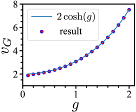
Figure 14: $g$ dependence of the sliding velocity $v_{G}=[x_{G}(t)-x_{G}(0)]/t$ in free particle dynamics: $W=0$; cf. Fig. 4 (a). From the same data as employed for producing Fig. 4 (a) data at $W=0$ is extracted and replotted as a function of $g$. To be compared with the formula (44). No disorder averaging ($\theta_{0}=0$); $j_{0}=580$. $L=601$.

Appendix B Free particle wave-packet dynamics in a non-Hermitian system with Im $\epsilon_{k}\neq 0$

Let us consider a free particle motion prescribed by the Hamiltonian (1). For simplicity, we switch off the quasi-periodic potential (2); $W=0$. In this disorder-free case, the eigenstates of the Hamiltonian (1) under the PBC take the form of a plane wave $e^{ik}$, while the corresponding eigenenergies $\epsilon_{k}$ become complex; see Eqs. (14), (15). Taking the initial state $|\psi(t=0)\rangle$ as in the main text; i.e., as in Eq. (7), we consider its time evolution Eq. (10). Considering the limit $L\rightarrow\infty$, we replace the summation over $k$ in the last line of Eq. (10) by an integral:

$$|\psi(t)\rangle=\sum_{j}|j\rangle\int^{2\pi}_{0}dk\frac{1}{\sqrt{2\pi}}e^{2i\cos(k-ig)t+ik(j_{0}-j)}.$$ (42)

At this point, let us recall that the one-body spectrum $\epsilon=\epsilon_{k}$ is complex as in Eq. (14), and its imaginary part Im $\epsilon_{k}$ becomes maximal at $k=k_{0}=-\frac{\pi}{2}$. Then, in the superposition of contributions from different $k$-components (the integral over $k$) in Eq. (42), the dominant contributions in time evolution stem from those around $k=k_{0}$, and such contributions govern the long time dynamics;

$$|\psi(t)\rangle \simeq \sum_{j}|j\rangle\int^{-\frac{\pi}{2}+\delta k}_{-\frac{\pi}{2}-\delta k}dk\frac{1}{\sqrt{2\pi}}e^{2i\cosh(g)(k+\frac{\pi}{2})t}$$ (43)

$$\times e^{2\sinh(g)(1-\frac{1}{2}(k+\frac{\pi}{2})^{2})t+i(k+\frac{\pi}{2})(j_{0}-j)}$$

$$\simeq \sum_{j}|j\rangle\int^{\infty}_{-\infty}dk\frac{1}{\sqrt{2\pi}}e^{2i\cosh(g)kt}$$

$$\times e^{2\sinh(g)(1-\frac{k^{2}}{2})t+ik(j_{0}-j)}$$

$$= \sum_{j}|j\rangle\exp(-\frac{((j_{0}-j)+2\cosh(g)t)^{2}}{4\sinh(g)t})$$

$$\times e^{2\sinh(g)t}/\sqrt{4\sinh(g)t}.$$

From the last expression, one can read (the $g$-dependence of) the group velocity of the wave packet as

$$v_{G}=2\cosh(g),$$ (44)

which seems also consistent with our numerics (Fig. 14). Note that $v_{G}$ increases with the increase of $g$.The last expression takes the form of a Gaussian wave packet that slides in the direction imposed by $g$, clearly demonstrating why the packet does not immediately spread, but rather slides. The expanse $\Delta x$ of the wave packet gradually increases in real space, though, in the course of time as $\Delta x\simeq 2\sqrt{\sinh(g)t}$, while the corresponding width $\Delta k\sim 1/\Delta x$ in the reciprocal space tends to diminish [see Fig. 3 (a)]. The above features are also quite manifest in panels (a-b) of Fig. 2 albeit in the panels a weak disorder is present. These are consequences of the fact that in the time evolution the state $|\psi(t)\rangle$ as given in Eq. (42), tends to be governed by the eigenstates with maximal Im $\epsilon_{k}$ [see Eq. (17)], while the individual eigenstates take spatially a form of plane wave.

Note that the form of the Gaussian wave packet (43) suggests that it obeys a square-root scaling typical to classical diffusion dynamics. Of course, we consider a coherent quantum dynamics of the wave function $\psi(x,t)$, which is governed by the Schrödinger equation. Here, however, in the present non-Hermitian setup, the asymmetric nature of the hopping strongly suppresses the interference of the complex wave function $\psi(x,t)$, characteristic to the Schrödinger quantum dynamics. As a result, the wave function $\psi(x,t)$ as given in Eq. (43) obeys effectively the classical diffusion dynamics. In the presence of random potential scatterers, different scattering paths are expected to interfere in spite of the asymmetric hopping; i.e., quantum interference may be partly recovered in this case. As a result, the system may exhibit a behavior analogous to the Hermitian case. Such an expectation is consistent with the appearance of the cascade-like enhancement of the wave-packet spreading in the regime of $W$ close to $W_{c}$ (see Sec. II).

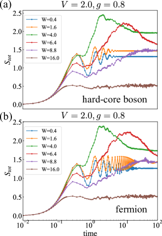
Figure 15: Time evolution of the entanglement entropy in the (a) hard-core boson and (b) fermion models. We employ same numerical parameters as in Fig. 10.

Appendix C Effects of anticommutation relation on the entanglement dynamics

So far we have considered systems of hard-core bosons; cf. Refs. Hamazaki et al., 2019, Zhai et al., 2020. In a system of true fermions, the anticommutation of $b_{j}$ and $b_{j}^{\dagger}$ gives rise to a subtle sign difference at the periodic boundary. Here, we examine whether this sign difference results in a significant consequence in the entanglement dynamics. Fig. 15(a) shows selected plots from Fig. 10 (i-b), which demonstrates time evolution of the entanglement entropy in the case of $g=0.8$ in the hard-core boson model. Fig. 15(b) represents corresponding data in the fermion model; under the same condition. In the critical and localized regimes: $W>3-4$, the wave functions are not extended, and the corresponding electronic states are expected to be immune to the sign difference. The result of our simulation in the fermionic case confirms that the entanglement entropy exhibits essentially the same behavior in the two models; i.e., the anticommutation relation plays no role in this regime. In the delocalized regime ($W<3-4$) the wave functions are extended over the entire system so that, in principle, the resulting electronic state may be influenced by the statistics. In this regime the entanglement entropy shows an oscillatory behavior in the intermediate time scale; a simple damped oscillation in the case of hard-core boson model. In the fermionic case one can still recognize a similar oscillatory pattern, but it does not look any longer a simple damped oscillation, and also survives longer than in the hard-core boson case. Thus, the anticommutation relation influences the behavior of the entanglement entropy in the delocalized regime at a quantitative level, but the qualitative statements on its behavior in the hard-core boson model can still be applicable to the fermionic case. The behavior of the entanglement entropy is essentially unchanged in the critical and localized regimes.

Appendix D The entanglement entropy in the ETH and MBL phases (Hermitian case)

Let us comment on the relation between the entanglement entropy and the localization length. The multifractal dimension $D_{2}$ given in Eq. (41) measures to what extent the eigenstates are localized in the Hilbert space; this is related to how much the wave functions are localized in real space. Thus, in the regime of strong disorder (and in the Hermitian case: $g=0$), $D_{2}$ behaves asymptotically as De Tomasi et al. (2021) $D_{2}\sim\log(\xi)$, where $\xi$ represents the localization length in real space. This implies that the true Fock space-localization $D_{2}=0$ is generally never achieved Macé et al. (2019); Tikhonov and Mirlin (2018); Orito and Imura (2021), since $\xi$ is generally finite in the localized phase, except in the limit $W\rightarrow\infty$.

Fock-space localization effectively restricts the available Hilbert space, thus affecting the maximal value of the entanglement entropy; cf. in the free case it is given by the Page value (39). In a more generic case with a finite $D_{2}$ it becomes,De Tomasi and Khaymovich (2020)

$$S_{\rm tot}\sim D_{\rm ent}{L\over 2}\log(2),$$ (45)

where $D_{\rm ent}$ is a quantity related to $D_{2}$:

$$D_{\rm ent}=\begin{cases}1,&D_{2}\geq 1/2\\ 2D_{2},&D_{2}<1/2.\end{cases}$$ (46)

i.e., on the ETH side: $D_{2}>1/2$ the reduction of the multifractal dimension $D_{2}$ due to a finite $W$ does not lead to reduction of the entanglement entropy $S_{\rm tot}$, while in the MBL side: $D_{2}<1/2$, $S_{\rm tot}$ decreases linearly with the decrease of $D_{2}$; in particular, $S_{\rm tot}$ does not show a finite jump at the ETH-MBL transition: $D_{2}=1/2$, and gradually crosses over from the ETH to the MBL side. In the time evolution of $S_{\rm tot}(t)$ plotted in Fig. 7 (a), its saturated value in the long time scale remains the same in the delocalized phase: $W\leq 2$, while in the localized phase: $W>2$, it decreases continuously from this value as $W$ is increased.

References

- Gornyi et al. (2005) I. V. Gornyi, A. D. Mirlin, and D. G. Polyakov, Phys. Rev. Lett. 95, 206603 (2005).
- Basko et al. (2006) D. Basko, I. Aleiner, and B. Altshuler, Annals of Physics 321, 1126 (2006).
- Bauer and Nayak (2013) B. Bauer and C. Nayak, Journal of Statistical Mechanics: Theory and Experiment 2013, P09005 (2013).
- Luitz et al. (2015) D. J. Luitz, N. Laflorencie, and F. Alet, Phys. Rev. B 91, 081103 (2015).
- Khemani et al. (2017) V. Khemani, S. P. Lim, D. N. Sheng, and D. A. Huse, Phys. Rev. X 7, 021013 (2017).
- Kjäll et al. (2014) J. A. Kjäll, J. H. Bardarson, and F. Pollmann, Phys. Rev. Lett. 113, 107204 (2014).
- Serbyn et al. (2016) M. Serbyn, A. A. Michailidis, D. A. Abanin, and Z. Papić, Phys. Rev. Lett. 117, 160601 (2016).
- Žnidarič et al. (2008) M. Žnidarič, T. c. v. Prosen, and P. Prelovšek, Phys. Rev. B 77, 064426 (2008).
- Bardarson et al. (2012) J. H. Bardarson, F. Pollmann, and J. E. Moore, Phys. Rev. Lett. 109, 017202 (2012).
- Serbyn et al. (2013) M. Serbyn, Z. Papić, and D. A. Abanin, Phys. Rev. Lett. 110, 260601 (2013).
- Agarwal et al. (2015) K. Agarwal, S. Gopalakrishnan, M. Knap, M. Müller, and E. Demler, Phys. Rev. Lett. 114, 160401 (2015).
- Bar Lev et al. (2015) Y. Bar Lev, G. Cohen, and D. R. Reichman, Phys. Rev. Lett. 114, 100601 (2015).
- Luitz et al. (2016) D. J. Luitz, N. Laflorencie, and F. Alet, Phys. Rev. B 93, 060201 (2016).
- Nandkishore and Huse (2015) R. Nandkishore and D. A. Huse, Annual Review of Condensed Matter Physics 6, 15 (2015).
- Alet and Laflorencie (2018) F. Alet and N. Laflorencie, Comptes Rendus Physique 19, 498 (2018).
- Abanin et al. (2019) D. A. Abanin, E. Altman, I. Bloch, and M. Serbyn, Rev. Mod. Phys. 91, 021001 (2019).
- Schreiber et al. (2015) M. Schreiber, S. S. Hodgman, P. Bordia, H. P. Luschen, M. H. Fischer, R. Vosk, E. Altman, U. Schneider, and I. Bloch, Science 349, 842–845 (2015).
- Choi et al. (2016) J.-y. Choi, S. Hild, J. Zeiher, P. Schauss, A. Rubio-Abadal, T. Yefsah, V. Khemani, D. A. Huse, I. Bloch, and C. Gross, Science 352, 1547–1552 (2016).
- Roushan et al. (2017) P. Roushan, C. Neill, J. Tangpanitanon, V. M. Bastidas, A. Megrant, R. Barends, Y. Chen, Z. Chen, B. Chiaro, A. Dunsworth, and et al., Science 358, 1175–1179 (2017).
- Smith et al. (2016) J. Smith, A. Lee, P. Richerme, B. Neyenhuis, P. W. Hess, P. Hauke, M. Heyl, D. A. Huse, and C. Monroe, Nature Physics 12, 907–911 (2016).
- Xu et al. (2018) K. Xu, J.-J. Chen, Y. Zeng, Y.-R. Zhang, C. Song, W. Liu, Q. Guo, P. Zhang, D. Xu, H. Deng, K. Huang, H. Wang, X. Zhu, D. Zheng, and H. Fan, Phys. Rev. Lett. 120, 050507 (2018).
- Deutsch (1991) J. M. Deutsch, Phys. Rev. A 43, 2046 (1991).
- Srednicki (1994) M. Srednicki, Phys. Rev. E 50, 888 (1994).
- Rigol et al. (2008) M. Rigol, V. Dunjko, and M. Olshanii, Nature 452, 854–858 (2008).
- Ros et al. (2015) V. Ros, M. Müller, and A. Scardicchio, Nuclear Physics B 891, 420 (2015).
- Imbrie et al. (2017) J. Z. Imbrie, V. Ros, and A. Scardicchio, Annalen der Physik 529, 1600278 (2017).
- Anderson (1958) P. W. Anderson, Phys. Rev. 109, 1492 (1958).
- Altshuler et al. (1997) B. L. Altshuler, Y. Gefen, A. Kamenev, and L. S. Levitov, Phys. Rev. Lett. 78, 2803 (1997).
- Roy et al. (2019) S. Roy, J. T. Chalker, and D. E. Logan, Phys. Rev. B 99, 104206 (2019).
- Roy and Logan (2020) S. Roy and D. E. Logan, Phys. Rev. B 101, 134202 (2020).
- Orito and Imura (2021) T. Orito and K.-I. Imura, Phys. Rev. B 103, 214206 (2021).
- Huse et al. (2014) D. A. Huse, R. Nandkishore, and V. Oganesyan, Phys. Rev. B 90, 174202 (2014).
- Hatano and Nelson (1996) N. Hatano and D. R. Nelson, Phys. Rev. Lett. 77, 570 (1996).
- Hatano and Nelson (1997) N. Hatano and D. R. Nelson, Phys. Rev. B 56, 8651 (1997).
- Hamazaki et al. (2019) R. Hamazaki, K. Kawabata, and M. Ueda, Phys. Rev. Lett. 123, 090603 (2019).
- Zhai et al. (2020) L.-J. Zhai, S. Yin, and G.-Y. Huang, Phys. Rev. B 102, 064206 (2020).
- Panda and Banerjee (2020) A. Panda and S. Banerjee, Phys. Rev. B 101, 184201 (2020).
- Longhi (2021) S. Longhi, Phys. Rev. B 103, 054203 (2021).
- Note (1) plays the same role as a damper in a Newtonian harmonic oscillator that tend to make the oscillation of the wave function damp in time. If () corresponds to hopping in the direction of positive , the eigen wave functions tend to damp with increasing , showing a damped harmonic oscillation, while the regime of corresponds to the case of an anti-damper; i.e., to an unrealistic parameter regime in the Newtonian model.
- Note (2) In non-Hermitian quantum mechanics with non-reciprocal hopping, choice of the boundary condition is a subtle issue, especially in its statics, while here, we are concerned about its dynamics in which the choice of the boundary condition is unlike in statics (see Appendix A for details) not a central issue.
- Note (3) Note that unlike the case of uncorrelated disorder; i.e., obeying a uniform distribution, the addition of disorder does not lead immediately to localization in the Aubry-Andre model; i.e., in the case of quasi-periodic disorder (2) even in the Hermitian limit: and despite the one dimensionality of the model. Abrahams et al. (1979) This will be a merit in the study of the entanglement entropy in the non-Hermitian case: , since one can always compare the situation at a finite with the Hermitian case: . In the case of uncorrelated disorder, the Hermitian limit becomes rather special.
- Aubry and André (1980) S. Aubry and G. André, Ann. Israel Phys. Soc. 3, 133 (1980).
- Note (4) In the practical calculation -averaging has been taken over samples; e.g., in the evaluation of and its fluctuation (Figs. 4, 6), and in the evaluation of different types entanglement entropies: , and .
- Note (5) The critical point (3) may be also understood from the viewpoint of the duality of the model.Deng et al. (2017).
- De Tomasi et al. (2021) G. De Tomasi, I. M. Khaymovich, F. Pollmann, and S. Warzel, Phys. Rev. B 104, 024202 (2021).
- Heußen et al. (2021) S. Heußen, C. D. White, and G. Refael, Phys. Rev. B 103, 064201 (2021).
-
Note (6)