On Homophony and Rényi Entropy

Abstract

Homophony's widespread presence in natural languages is a controversial topic. Recent theories of language optimality have tried to justify its prevalence, despite its negative effects on cognitive processing time; e.g., Piantadosi et al. (2012) argued homophony enables the reuse of efficient wordforms and is thus beneficial for languages. This hypothesis has recently been challenged by Trott and Bergen (2020), who posit that good wordforms are more often homophonous simply because they are more phonotactically probable. In this paper, we join in on the debate. We first propose a new information-theoretic quantification of a language's homophony: the sample Rényi entropy. Then, we use this quantification to revisit Trott and Bergen's claims. While their point is theoretically sound, a specific methodological issue in their experiments raises doubts about their results. After addressing this issue, we find no clear pressure either towards or against homophony—a much more nuanced result than either Piantadosi et al.'s or Trott and Bergen's findings.

1 Introduction

Ambiguity is a hallmark of human language, and is present at all levels of linguistic structure. Both the causes and resulting effects of ambiguity are topics which have sparked much debate. For example, while some claim it has a beneficial impact on communication, others have taken it as a sign of inefficiency. In this work, we contribute to the debate surrounding a specific form of lexical ambiguity in which a wordform shares multiple unrelated meanings: homophony.

While the quantitative study of homophony dates back to (at least) Zipf (1949), recently, Trott and Bergen (2020) proposed a new explanation for the higher rate of homophony amongst good, i.e. short or phonotactically well-formed, wordforms: if words were sampled i.i.d. from a phonotactic distribution, then good wordforms would simply be sampled more often. This implies there is no pressure favouring homophony in these words for the sake of efficiency, which directly opposes Piantadosi et al.'s (2012) hypothesis. In fact, Trott and Bergen go further, relying on their experimental results to argue that ``homophony may even be selected against in real languages.''

In this work, we join this debate by proposing a novel quantification of a language's homophony: the sample Rényi entropy—defined as the negative log likelihood (or surprisal) that two instances in an $M$-sized sample take on the same value. When measured on an observed lexicon, this measure holistically captures the chance that two wordforms coincide, i.e., that they are homophones, providing a new means to test whether lexicons have a pressure in favour or against homophony.

Further, we revisit Trott and Bergen's claims. Whilst their theoretical arguments are sound, we believe their experimental design could not have provided concrete evidence for or against their hypothesis. Specifically, their inadequate modelling of the phonotactic distribution, through the use of weakly regularised $n$-grams, cause us to question conclusions drawn from their experiments. We take measures to address this issue—relying on more expressive LSTM language models—and provide our own analysis of homophony in natural language.

Experimentally, we arrive at more nuanced results than prior work, finding no pressure either towards or against homophony. We conclude with the warning that biases in our models—and those of other works—need to be deeply considered when relying on them to answer linguistics questions.

2 Homophony

Homophony is a widespread phenomenon which has long puzzled linguists. On average, roughly $4\%$ of the words in a language are estimated to be homophones (Dautriche, 2015). This rate, however, has a large variation across languages—in English, for instance, Rodd et al. (2002) estimates it to be $7.4\%$. A number of works hint at the inefficiencies homophony leads to: Rodd et al. (2002) find that homophonous words are recognised more slowly; Mazzocco (1997) shows homophones are harder for children to learn.

Yet a large body of work has argued for the efficiency of homophony. Piantadosi et al. (2012) suggest ambiguity is a desirable property in that it increases a language's communicative efficiency. Ambiguity would allow a language to reuse good wordforms, which falls in line with Zipf's principle of least effort. With this in mind, Piantadosi et al. showed that short, frequent and phonotactically probable wordforms have more homophones than their counterparts. In further support of this hypothesis, Dautriche et al. (2018) found children easily learn to differentiate homophones when pairs have distinct syntactic categories (and that homophony is more likely in these cases); Pimentel et al. (2020a) showed speakers make contexts more informative in the presence of lexical ambiguity. These results suggest people naturally navigate ambiguity.

However, Trott and Bergen recently proposed a new explanation of Piantadosi et al.'s findings: They attribute homophony to chance. Specifically, they claim that if we model the phonotactic distribution probabilistically, we can see that more homophones amongst good wordforms should be expected—they are simply more probable. Yet their methodology to support this claim—comparing natural lexicons with artificial ones sampled from $n$-gram language models—has an important setback: their use of 5-gram models with only weak Laplace smoothing. These models are prone to overfitting. As such, it is not surprising that an artificially generated lexicon would contain more homophony than natural ones; as we will show, overfit distributions will likely produce more collisions. Thus, it is not entirely clear what we can conclude from their experiments.

3 Quantifying Homophony

As per its definition, homophony should be tightly related to a language's phonotactics—its distribution over wordforms. In this section, we first provide a definition of a language's phonotactic distribution. We then present both the Rényi collision entropy and the sample Rényi entropy as new measures of homophony.

3.1 Phonotactics and Wordforms

Formally, phonotactics defines a language's set of plausible wordforms. Its classic exemplification, provided by Chomsky and Halle (1965), is that while the unattested wordform blick would be plausible in English, *bnick would not. Under a probabilistic interpretation (Hayes and Wilson, 2008; Gorman, 2013), this can be re-stated as blick having high phonotactic probability, while *bnick has low phonotactic probability. Notedly, a language's phonotactics highly constrains its set of possible wordforms (Dautriche et al., 2017a) and, cross-linguistically, the size of these sets seems to be roughly constant (Pimentel et al., 2020b). Further, phonotactics has a tight relationship with word frequency; more phonotactically likely words are more frequent (Mahowald et al., 2018).

We model the phonotactic distribution over possible wordforms as a language model:

$$p(\mathbf{w})=\prod_{t=1}^{|\mathbf{w}|}p(w_{t}\mid\mathbf{w}_{<t})$$ (1)

whose support is the infinite set $\mathcal{W}$—defined here as the Kleene closure of a phonetic alphabet $\Sigma^{*}$, albeit where all $\mathbf{w}\in\mathcal{W}$ are padded with beginning-of- and end-of-word symbols. Under this definition, highly plausible wordforms would be assigned high probability, and vice-versa.

3.2 Entropy as a Measure of Homophony

The Rényi entropy is a generalisation of the more well-known Shannon entropy. By its information-theoretic definition, a natural parallel can be drawn between Rényi entropy and homophony. Its general form is defined as

$$\mathrm{H}_{\alpha}(p)=\frac{1}{1-\alpha}\log\left(\sum_{\mathbf{w}\in\mathcal{W}}p(\mathbf{w})^{\alpha}\right)$$ (2)

for $\alpha\geq 0,\neq 1$. If we take the limit $\alpha\rightarrow 1$, we recover the Shannon entropy:

$$\mathrm{H}_{1}(p)=-\sum_{\mathbf{w}\in\mathcal{W}}p(\mathbf{w})\log p(\mathbf{w})$$ (3)

which captures the inherent uncertainty in a distribution, i.e. the larger its value, the less predictable the outcome. The case of $\alpha=2$ yields the collision entropy (sometimes just termed the Rényi entropy)

$$\mathrm{H}_{2}(p)=-\log\sum_{\mathbf{w}\in\mathcal{W}}p(\mathbf{w})^{2}$$ (4)

which, in our setting, is the negative log likelihood that two wordforms sampled i.i.d. from the same distribution are the same. It thus provides a natural quantification of homophony in a language where the words are distributed i.i.d.

Although both the collision and Shannon's entropies are measures of uncertainty, they capture distinct properties of the distribution. Shannon's entropy represents the expected surprisal of observing any specific wordform $\mathbf{w}$, while the collision entropy computes the surprisal that a pair of words have identical forms, independent of which form.

3.3 Measuring Collisions in a Lexicon

In the previous section, we presented the Rényi collision entropy as measured on a specific phonotactic distribution. The measure in eq. 4 has the unstated assumption that a pair of wordforms would be sampled i.i.d. from this distribution—i.e., the probability of a collision is $p(\mathbf{w})^{2}$, as opposed to $p(\mathbf{w}^{(1)})p(\mathbf{w}^{(2)}\mid\mathbf{w}^{(1)})$. We do not, however, know if this i.i.d. assumption is valid for naturally occurring lexica. We thus propose a new measure, termed the sample Rényi entropy, which does not inherently encode an i.i.d. assumption. Given an observed lexicon $\widetilde{\mathbf{W}}=\{\widetilde{\mathbf{w}}^{(m)}\}_{m=1}^{M}$ of size $M$, we directly measure the surprisal of two randomly selected words being a homophone as

$$\mathrm{R}( \widetilde{\mathbf{W}})=$$ (5)

$$-\log\frac{\sum\limits_{m=1}^{M}\,\,\sum\limits_{m^{\prime}=1,m^{\prime}\neq m}^{M}\mathbbm{1}\left\{\widetilde{\mathbf{w}}^{(m)}=\widetilde{\mathbf{w}}^{(m^{\prime})}\right\}}{M(M-1)}$$

In words, the above equation estimates the likelihood of a collision as the number of observed homophones over the number of possible collisions.

Notably, if words are sampled i.i.d.—i.e., if there is no pressure in favour or against homophony—the sample Rényi entropy goes to the actual Rényi entropy in eq. 4 as $M\rightarrow\infty$. In other words, under the i.i.d. assumption, eq. 5 is a consistent estimator of eq. 4.

3.4 A Tractable Estimate of Rényi Entropy

Note that in our setting, it is impossible to exactly calculate the Rényi entropy $\mathrm{H}_{2}(p)$, given that the support of $p$ (i.e., $\mathcal{W}$) is infinite. In this work, we estimate $\widehat{\mathrm{H}}_{2}(p)$ over a subset $\mathcal{W}_{\delta}\subset\mathcal{W}$:

$$\widehat{\mathrm{H}}_{2}(p)=-\log\sum_{\mathbf{w}\in\mathcal{W}_{\delta}}p(\mathbf{w})^{2}$$ (6)

Fortunately, we can show a tight bound on the approximation when the finite $\mathcal{W}_{\delta}$ is chosen wisely.

Theorem 3.1.

Let $\mathcal{W}_{\delta}$ be the set of all wordforms with a probability of at least $\delta$, i.e. $\mathcal{W}_{\delta}=\{\mathbf{w}\mid\mathbf{w}\in\mathcal{W},p(\mathbf{w})\geq\delta\}$. We can bound our estimate error as:

$$\mathrm{H}_{2}(p) \leq\widehat{\mathrm{H}}_{2}(p)\leq\mathrm{H}_{2}(p)+\log\left(1+\frac{(1-\xi)\,\delta}{\eta}\right)$$

where we can precisely compute both $\xi$ and $\eta$, which are defined as $\xi=\sum_{\mathbf{w}\in\mathcal{W}_{\delta}}p(\mathbf{w})$ and $\eta=\sum_{\mathbf{w}\in\mathcal{W}_{\delta}}p(\mathbf{w})^{2}$.

Proof.

Proof is given in App. D. ∎

This theorem implies $\widehat{\mathrm{H}}_{2}(p)$ is an upper bound on the true value $\mathrm{H}_{2}(p)$, which can be made arbitrarily tight for small $\delta$ (we choose $\delta=10^{-8}$ here).

3.5 A Null Hypothesis Test

We now construct a null-hypothesis test to evaluate whether the observed lexicon is shaped by pressures in favour or against homophony. Our null distribution over lexica of size $M$ is defined as

$$p(\mathbf{W})=\prod_{m=1}^{M}p(\mathbf{w}^{(m)})$$ (7)

where $p(\mathbf{w})$ is a phonotactic distribution. We further define a second distribution over values of the sample Rényi entropy, i.e. $p(\mathrm{R}(\mathbf{W}))$, where $\mathbf{W}$ is distributed according to $p(\mathbf{W})$. We can now ask whether the Rényi entropy in the observed lexicon is abnormal under the null distribution. This suggests the following null hypothesis test:

• $T_{0}$: $\mathrm{R}(\widetilde{\mathbf{W}})$ is sampled from $p(\mathrm{R}(\mathbf{W}))$

• $T_{1}$: $\mathrm{R}(\widetilde{\mathbf{W}})$ is not sampled from $p(\mathrm{R}(\mathbf{W}))$

For a given $p(\mathbf{W})$, we can now test this hypothesis by evaluating the following probabilities:

$$p(\mathrm{R}(\mathbf{W})\leq\mathrm{R}(\widetilde{\mathbf{W}}))\text{ or }p(\mathrm{R}(\mathbf{W})\geq\mathrm{R}(\widetilde{\mathbf{W}}))$$ (8)

which we can estimate using Monte Carlo sampling. We reject the null hypothesis if either probability is smaller than $0{.}005$, which yields a confidence value of $p<0{.}01$ under a two-tailed test. Strictly speaking, rejecting $T_{0}$, means that we have rejected that the sample Rényi entropy of the observed lexicon is plausibly consistent with the sample Rényi entropy of a lexicon sampled according to the null distribution $p(\mathbf{W})$.

We now analyse the assumptions we make by using $p(\mathbf{W})$ and discuss what conclusions we may be able to draw despite those assumptions. The two important assumptions are as follows:

1. wordforms are sampled according to $p(\mathbf{w})$;

2. wordforms are sampled i.i.d.

Therefore, if we believe our phonotactic distribution is correct—i.e., assumption (i) is good—this null hypothesis directly tests whether wordforms are sampled i.i.d. Rejecting it, thus, gives us evidence that homophony is either favoured or hindered in a lexicon. Should we believe assumption (i), we find evidence in support of homophony avoidance if the observed lexicon's sample Rényi entropy is significantly larger than the artificial one's. On the other hand, we find evidence of a pressure in favour of homophony if the observed lexicon's sample Rényi entropy is smaller than its artificial counterpart. Assumption (i) is rather important, however, as we discuss further in § 5.

4 Experimental Methodology

The sample Rényi entropy, presented in eq. 5, can be directly computed on an observed lexicon. On the other hand, both the Rényi entropy (as depicted in § 3.2) and our null hypothesis test are computed over a phonotactic distribution, to which we do not have direct access. An important consideration, thus, is how exactly this distribution can be approximated. Recently, Trott and Bergen (2020) relied on weakly regularised $n$-gram models for their analysis. As can be seen in our earlier results (Pimentel et al., 2020b), neural language models can capture this phonotactic distribution much more faithfully. In this work, we will compare Trott and Bergen's $n$-grams with Pimentel et al.'s LSTM models, and show how $n$-grams may give misleading results.

$n$-gram.

Perhaps the simplest method for estimating distributions of phones in a language is through $n$-gram, or in this case $n$-phone, modelling. Specifically, we can estimate the probability of observing some phone $w_{t}$ given the previous $n-1$ phones by computing the proportion of times this phone follows those previous $n-1$ phones in a corpus. By this definition, sequences not present in the corpus will be assigned $0$ probability under the model. This, among other factors, contributes to the often poor generalisation abilities of basic $n$-gram models. Indeed, there exists an entire literature on smoothing and regularisation techniques for $n$-gram modelling Katz (1987); Ney et al. (1994); Chen and Goodman (1996). Laplace smoothing is a popular choice, being used in a number of recent works in computational linguistics (e.g. Dautriche et al., 2017a; Trott and Bergen, 2020). However, it is perhaps the simplest of such regularisation techniques, and usually leads to much weaker empirical performances than, e.g., Kneyser–Ney (Ney et al., 1994). It is therefore natural to question whether an $n$-gram model with simple Laplace smoothing can provide a good representation of the true phonotactic distribution of a language. In our experiments, we follow Trott and Bergen in using a 5-gram model with Laplace smoothing with strength $0.01$ as $p(w_{t}\mid\mathbf{w}_{<t})$.

LSTM.

In the task of sentence-level language modelling, neural models have surpassed their $n$-gram counterparts with respect to standard evaluation metrics. Neural architectures similarly outperform an $n$-phone model on the task of representing the phonotactic distribution. We thus make use of a vanilla LSTM character-level language model to estimate this distribution, using a similar architecture to Pimentel et al.'s (2020b). In short, we first retrieve a lookup embedding $\mathbf{z}_{t}\in\mathbb{R}^{e}$ for each phone $w_{t}$ in a wordform. We then feed these into an LSTM (Hochreiter and Schmidhuber, 1997) to get hidden states $\mathbf{h}_{t}\in\mathbb{R}^{d}$. Finally, these hidden states are linearly transformed and processed by a softmax to arrive at a distribution $p(w_{t}\mid\mathbf{w}_{<t})$ over the next token. We train this model by minimising its cross-entropy with the distribution of the observed data. We use an LSTM architecture with 2 layers, an embedding size of 64, a hidden size of 256, and dropout probability of .33. This model is implemented using PyTorch (Paszke et al., 2019) and optimised using Adam (Kingma and Ba, 2015).

Model Selection.

We evaluate the quality of our models by measuring their cross-entropy on held-out data, as is common in language modelling. We report their train and test cross-entropies in Table 1. Note that minimising this cross-entropy is equivalent to minimising the Kullback–Leibler divergence between our estimated model and the actual phonotactic distribution. Thus, this serves as a metric of how well our model fits the data.

Data.

We use CELEX (Baayen et al., 1995) as the source of data for our experiments, a dataset which covers three languages (English, German, and Dutch). We restrict our analysis to mono-morphemic words, and note that we count words with multiple parts of speech as homophones (as both Piantadosi et al. and Trott and Bergen do). This may inflate the number of homophones in our actual lexicons, thus reducing their surprisal in our analysis. CELEX, however, marks zero derivation forms; we thus do not use these words on our analysis. When computing the plug-in estimate of the lexicon's Rényi entropy (in eq. 5) we use our entire dataset. We further use these wordforms to train our phonotactic models, splitting them in 80-10-10 train-validation-test sets. The test set is held out and only used for estimating the cross-entropy.

5 Results, Discussion and Conclusion

Table 1 displays our main results: first we note that in terms of cross-entropy, the LSTM models provide better representations of the phonotactic distributions of all three languages. Second, the Shannon entropy of the LSTM is smaller than the entropy of the $n$-gram. The $n$-gram, thus, appears to distribute probability mass more uniformly over the set $\mathcal{W}$ than the LSTM, while the LSTM is more focused on the set of plausible wordforms.

		Cross-entropy
		Train	Test	$\mathrm{H}_{1}(p)$	$\mathrm{H}_{2}(p)$	$\mathrm{R}(\mathbf{W})$
English	$n$-gram	13.61	28.10	30.45	13.89	13.90∗
	LSTM	18.75	19.89	26.46	14.77	14.77∗
	Lexicon	-	-	-	-	15.02∗
German	$n$-gram	14.08	29.25	30.44	14.27	14.27∗
	LSTM	20.26	21.35	27.74	15.87	15.88∗
	Lexicon	-	-	-	-	15.67∗
Dutch	$n$-gram	13.89	26.08	30.45	14.07	14.06∗
	LSTM	18.37	18.94	26.81	15.16	15.16∗
	Lexicon	-	-	-	-	14.60∗
∗Statistically different from lexicon's Rényi entropy ($p<0.01$).

Table 1: Cross-entropy, Shannon's entropy and Rényi entropy for both the $n$-gram, LSTM and lexicon.

The Rényi collision entropy results must be more carefully analysed. At first glance, we see that the $n$-gram model has the smallest Rényi entropy across all languages, having more than 1 bit difference to the lexicon's sample Rényi entropy in both English and German. This may lead one to conclude that homophony is strongly disfavoured in all these languages. Nonetheless, the LSTM's collision entropy is considerably larger than the $n$-gram model's, while having both a lower cross-entropy and Shannon entropy. We posit this is due to the $n$-gram strongly overfitting the training set, giving these instances a higher probability than they are due. These few overfit wordforms drive its Rényi entropy down, while the rest of the probability mass is spread over $\mathcal{W}$ and increases the $n$-gram's Shannon entropy. In other words, $n$-gram models do not approximate $p(\mathbf{w})$ well, and the assumption (i) of our hypothesis test does not hold.

When we compare the Rényi entropy of the LSTM to the lexicon's, we get much more nuanced results. While the English lexicon seems to hinder homophony—homophony is more surprising in real lexicons than expected from their phonotactics—the opposite is true for Dutch. Meanwhile, German presents no clear trends. We should, however, refrain from making strong claims about these results. While the difference between the LSTM's train and test cross-entropy is small, implying that it overfits only to a small degree, its precise quantitative impact on the Rényi entropy is hard to quantify. Furthermore, expanding our analysis to CELEX's multi-morphemic words leads to somewhat different results (see App. B). Hence, we see no clear pattern across these languages, and find, thus, no pressure either in favour or against homophony.

We conclude this section with a warning. When exploring linguistics using language models, one should carefully consider these model's inherent inductive biases and their potential effects on results. While overfit $n$-grams provide strong evidence towards homophony avoidance in natural lexicons, we arrive at different results using better models.

Ethical Considerations

The authors foresee no ethical concerns with the research presented in this paper.

Appendix A More Related Work

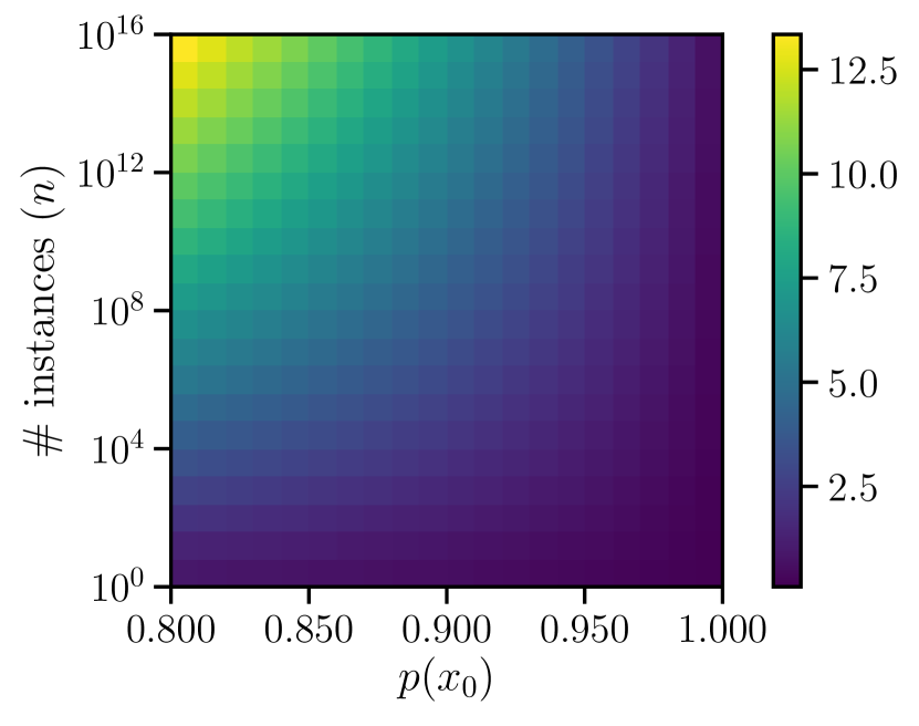
(a) Shannon entropy

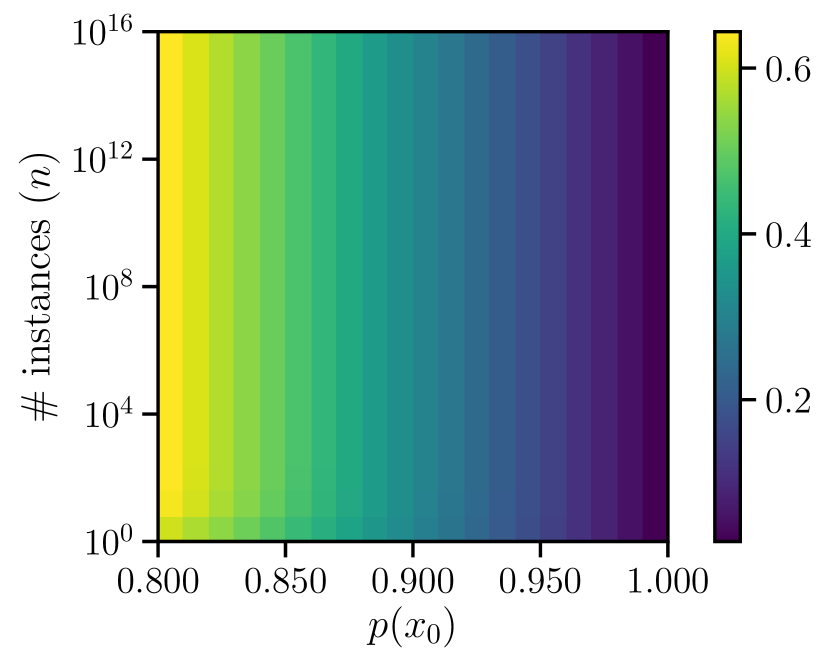
(b) Rényi entropy

Figure 1: Shannon and Rényi collision entropies for a distribution where one instance has probability $p(x_{0})$ and another $n$ instances have probability mass uniformly distributed among them.

Related to the topic of homophony is the debate surrounding the effect of lexical neighbourhoods in the lexicon—of which homophony can potentially be seen as an extreme case. While dense lexical neighbourhoods may hinder lexical recognition (Luce, 1986; Luce and Pisoni, 1998; Magnuson et al., 2007), a dense phonotactic space would imply more economic wordforms (Zipf, 1949; Piantadosi et al., 2011). Furthermore, phonotactically well-formed words are both recognised faster (Vitevitch et al., 1999) and easier for young children to learn (Coady and Aslin, 2004). It is thus not clear if denser lexical neighbourhoods would lead to a more or less ``efficient'' lexicon. Dautriche et al. (2017a) showed, using a very similar methodology to Trott and Bergen's (2020), that words have more phonological neighbours than would be expected by chance. Their results, though, are vulnerable to similar criticisms to the ones that we provide in this paper about the use of potentially overfit $n$-gram models.

Caplan et al. (2020) propose a phonotactic monkey—an extension of Miller's (1957) random typing thought experiment—to make a similar point to Trott and Bergen. They rely on similar $n$-gram phonotactic models for their analysis of homophony, being thus vulnerable to the same criticisms we present here. Caplan et al., however, refrain from making claims about a pressure towards or against homophony—positing homophony is only a result of chance, a byproduct of language's generation process. Caplan et al. further analyse polysemy in their paper, a topic with which we do not engage here. Incorporating form–meaning interactions to this analysis is not straightforward, but would be interesting as future work. We believe, however, that when studying homophony, ignoring them is not particularly problematic, since the multiple meanings a wordform takes are unrelated by definition. Nonetheless, it would be critical to incorporate meaning in our model if we wanted to study other forms of lexical ambiguity. Furthermore, several recent work has shown that the lexicon is (weakly) systematic, i.e. words with similar meanings are more likely to have similar wordforms (Dautriche et al., 2017b; Gutiérrez et al., 2016; Pimentel et al., 2019). Our i.i.d. use of a phonotactic distribution, though, completely ignores these form–meaning correlations.

Appendix B Multi-morphemic results

		Cross-entropy
		Train	Test	$\mathrm{H}_{1}(p)$	$\mathrm{H}_{2}(p)$	$\mathrm{R}(\mathbf{W})$
English	$n$-gram	17.97	27.16	29.74	16.07	16.07∗
	LSTM	25.00	25.55	28.92	17.97	17.96∗
	Lexicon	-	-	-	-	16.67∗
German	$n$-gram	20.37	29.67	31.39	15.69	15.69∗
	LSTM	27.51	27.94	31.55	18.85	18.85∗
	Lexicon	-	-	-	-	19.91∗
Dutch	$n$-gram	23.03	30.61	31.81	15.37	15.37∗
	LSTM	29.37	29.76	30.99	19.54	19.54∗
	Lexicon	-	-	-	-	20.57∗
∗Statistically different from lexicon's Rényi ($p<0.01$).

Table 2: Cross-entropy, Shannon's entropy and Rényi entropy for both the $n$-gram, LSTM and real lexicon while also analysing multi-morphemic wordforms.

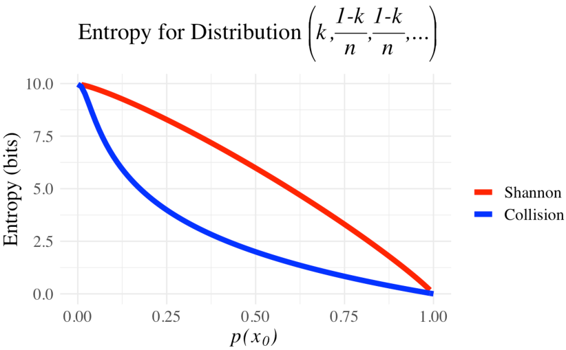
Figure 2: Shannon and Rényi collision entropies for distribution with uniform mass spread over all but one instance.

Appendix C Shannon vs. Collision Entropy

In this section, we exemplify the difference between the Rényi and Shannon entropies. With that in mind, we define a distribution over $n+1$ instances, where probability mass is distributed such that:

$$p(x)=\left\{\begin{array}[]{cc}k&x=x_{0}\\ \frac{1-k}{n}&x\neq x_{0}\end{array}\right.$$ (11)

This distribution, thus, puts $k$ probability mass on $x_{0}$, and uniformly distributes the rest among the $n$ other instances.

Figure 2 shows the behaviour of both entropies with $n$ fixed at $99$ and while we vary the mass in $p(x_{0})$. In it, we see how the Rényi entropy is always smaller or equal to the Shannon entropy—an important property of the Rényi collision entropy.

Figure 1 presents these entropies while changing both $n$ and $k$, i.e. $p(x_{0})$. In this figure, we see that when some large probability mass is already allocated to a single instance (or a few), the Rényi entropy becomes relatively constant with relation to the distribution among the other instances. The Shannon entropy, on the other hand, is still susceptible to these other instances distribution, and goes to infinity as $n\rightarrow\infty$.

Relating this to our analysed $n$-gram models, we see that, by allocating a large probability mass to the training set, they can obtain a small Rényi entropy. However, since they smoothly distribute the rest of their probability mass throughout $\mathcal{W}$ they achieve a high Shannon entropy.

Appendix D Proof of theorem 3.1

Theorem 3.1. Let $\mathcal{W}_{\delta}$ be the set of all wordforms with a probability at least $\delta$, i.e.

$$\mathcal{W}_{\delta}=\{\mathbf{w}\mid\mathbf{w}\in\mathcal{W},p(\mathbf{w})\geq\delta\}$$

We can bound our estimate error as:

$$\mathrm{H}_{2}(p) \leq\widehat{\mathrm{H}}_{2}(p)\leq\mathrm{H}_{2}(p)+\log\left(1+\frac{(1-\xi)\,\delta}{\eta}\right)$$

where we can precisely compute both $\xi$ and $\eta$, which are defined as

$$\xi=\sum_{\mathbf{w}\in\mathcal{W}_{\delta}}p(\mathbf{w}),\qquad\eta=\sum_{\mathbf{w}\in\mathcal{W}_{\delta}}p(\mathbf{w})^{2}$$

Proof.

We first decompose the error in our estimate as

$$\widehat{\mathrm{H}}_{2}(p)-\mathrm{H}_{2}(p) \stackrel{{\scriptstyle(1)}}{{=}}\log\left(\sum_{\mathbf{w}\in\mathcal{W}_{\delta}}p(\mathbf{w})^{2}+\sum_{\mathbf{w}\in\mathcal{W}\setminus\mathcal{W}_{\delta}}p(\mathbf{w})^{2}\right)-\log\left(\sum_{\mathbf{w}\in\mathcal{W}_{\delta}}p(\mathbf{w})^{2}\right)$$ (12a)

$$=\log\left(\frac{\sum_{\mathbf{w}\in\mathcal{W}_{\delta}}p(\mathbf{w})^{2}+\sum_{\mathbf{w}\in\mathcal{W}\setminus\mathcal{W}_{\delta}}p(\mathbf{w})^{2}}{\sum_{\mathbf{w}\in\mathcal{W}_{\delta}}p(\mathbf{w})^{2}}\right)$$ (12b)

$$=\log\left(1+\frac{\sum_{\mathbf{w}\in\mathcal{W}\setminus\mathcal{W}_{\delta}}p(\mathbf{w})^{2}}{\eta}\right)$$ (12c)

where $\eta=\sum_{\mathbf{w}\in\mathcal{W}_{\delta}}p(\mathbf{w})^{2}$ and equality (1) follows from the definition of $\mathrm{H}_{2}$ and the separation of the sum into two parts. We define $\xi=\sum_{\mathbf{w}\in\mathcal{W}_{\delta}}p(\mathbf{w})$ and, thus, $1-\xi=\sum_{\mathbf{w}\in\mathcal{W}\setminus\mathcal{W}_{\delta}}p(\mathbf{w})$. Now, by invoking Lemma D.1, we have the following inequality

$$0\leq\sum_{\mathbf{w}\in\mathcal{W}\setminus\mathcal{W}_{\delta}}p(\mathbf{w})^{2} \leq\left(1-\xi\right)\delta$$ (13)

which proves the theorem.

∎

Lemma D.1.

(Technical Lemma) Let $\{x_{n}\}_{n=1}^{N}$ be real values in the interval $[0,\delta]$ such that $\sum_{n=1}^{N}x_{n}=\beta$. Then,

$$\sum_{n=1}^{N}x_{n}^{2}\leq\beta\cdot\delta$$ (14)

Proof.

We claim the maximal solution—i.e., the set $\{x_{n}\}_{n=1}^{N}$ which maximises eq. 14—is $x_{k}=\delta$ for $k\in 1,\ldots,K$ and $x_{K+1}=\beta-K\delta$ for some $K<N$. We prove its maximality by contradiction. Suppose there exists another maximal solution. Further, suppose that the values for this solution are sorted, such that $x_{i}\geq x_{j}$ for any $i<j$. Then, there must exist two indices $i$ and $j$ such that $\delta>x_{i}\geq x_{j}$ and $i<j$. Now, let $\epsilon=\delta-x_{i}>0$. We can prove that:

$$(x_{i}+\epsilon)^{2}+(x_{j}-\epsilon)^{2} =x_{i}^{2}+2x_{i}\epsilon+\epsilon^{2}+x_{j}^{2}-2x_{j}\epsilon+\epsilon^{2}$$ (15a)

$$=x_{i}^{2}+x_{j}^{2}+2\underbrace{(x_{i}-x_{j})}_{\geq 0}\epsilon+2\epsilon^{2}$$ (15b)

$$\stackrel{{\scriptstyle(1)}}{{>}}x_{i}^{2}+x_{j}^{2}$$ (15c)

where (1) relies on the fact that, per our assumptions, $\epsilon>0$ and $x_{i}\geq x_{j}$. Since this is a strict inequality, this alternate solution is not truly maximal, completing our proof by contradiction.

Now, we can use our maximal solution to compute the desired upper-bound. First, we note the value of $K=\left\lfloor\frac{\beta}{\delta}\right\rfloor$. The value for the maximal solution will thus be

$$\sum_{n=1}^{N}x_{n}^{2} =K\cdot\delta^{2}+\left(\beta-K\delta\right)^{2}$$ (16a)

$$=\left\lfloor\frac{\beta}{\delta}\right\rfloor\cdot\delta^{2}+\left(\beta-\left\lfloor\frac{\beta}{\delta}\right\rfloor\delta\right)^{2}$$ (16b)

$$=\left\lfloor\frac{\beta}{\delta}\right\rfloor\cdot\delta^{2}+\underbrace{\left(\beta-\left\lfloor\frac{\beta}{\delta}\right\rfloor\delta\right)}_{\geq 0}\underbrace{\left(\beta-\left\lfloor\frac{\beta}{\delta}\right\rfloor\delta\right)}_{<\delta}$$ (16c)

$$\leq\left\lfloor\frac{\beta}{\delta}\right\rfloor\cdot\delta^{2}+\left(\beta-\left\lfloor\frac{\beta}{\delta}\right\rfloor\delta\right)\cdot\delta$$ (16d)

$$=\left\lfloor\frac{\beta}{\delta}\right\rfloor\cdot\delta^{2}+\left(\frac{\beta}{\delta}\delta-\left\lfloor\frac{\beta}{\delta}\right\rfloor\delta\right)\cdot\delta$$ (16e)

$$=\left\lfloor\frac{\beta}{\delta}\right\rfloor\cdot\delta^{2}+\left(\frac{\beta}{\delta}-\left\lfloor\frac{\beta}{\delta}\right\rfloor\right)\cdot\delta^{2}$$ (16f)

$$=\beta\cdot\delta$$ (16g)

As the value of the maximal solution is bounded by $\beta\cdot\delta$, any other solution must also have a value smaller than this, which completes the proof.

∎

References

- Baayen et al. (1995) R. Harald Baayen, Richard Piepenbrock, and Leon Gulikers. 1995. The CELEX lexical database (release 2). Linguistic Data Consortium.
- Caplan et al. (2020) Spencer Caplan, Jordan Kodner, and Charles Yang. 2020. Miller's monkey updated: Communicative efficiency and the statistics of words in natural language. Cognition, 205:104466.
- Chen and Goodman (1996) Stanley F. Chen and Joshua Goodman. 1996. An empirical study of smoothing techniques for language modeling. In 34th Annual Meeting of the Association for Computational Linguistics, pages 310–318, Santa Cruz, California, USA. Association for Computational Linguistics.
- Chomsky and Halle (1965) Noam Chomsky and Morris Halle. 1965. Some controversial questions in phonological theory. Journal of Linguistics, 1(2):97–138.
- Coady and Aslin (2004) Jeffry A. Coady and Richard N. Aslin. 2004. Young children's sensitivity to probabilistic phonotactics in the developing lexicon. Journal of Experimental Child Psychology, 89(3):183–213.
- Dautriche (2015) Isabelle Dautriche. 2015. Weaving an ambiguous lexicon. Ph.D. thesis, Sorbonne Paris Cité.
- Dautriche et al. (2018) Isabelle Dautriche, Laia Fibla, Anne-Caroline Fievet, and Anne Christophe. 2018. Learning homophones in context: Easy cases are favored in the lexicon of natural languages. Cognitive Psychology, 104:83–105.
- Dautriche et al. (2017a) Isabelle Dautriche, Kyle Mahowald, Edward Gibson, Anne Christophe, and Steven T. Piantadosi. 2017a. Words cluster phonetically beyond phonotactic regularities. Cognition, 163:128–145.
- Dautriche et al. (2017b) Isabelle Dautriche, Kyle Mahowald, Edward Gibson, and Steven T. Piantadosi. 2017b. Wordform similarity increases with semantic similarity: An analysis of 100 languages. Cognitive Science, 41(8):2149–2169.
- Gorman (2013) Kyle Gorman. 2013. Generative phonotactics. Ph.D. thesis, University of Pennsylvania.
- Gutiérrez et al. (2016) E. Dario Gutiérrez, Roger Levy, and Benjamin Bergen. 2016. Finding non-arbitrary form-meaning systematicity using string-metric learning for kernel regression. In Proceedings of the 54th Annual Meeting of the Association for Computational Linguistics (Volume 1: Long Papers), pages 2379–2388, Berlin, Germany. Association for Computational Linguistics.
- Hayes and Wilson (2008) Bruce Hayes and Colin Wilson. 2008. A maximum entropy model of phonotactics and phonotactic learning. Linguistic Inquiry, 39(3):379–440.
- Hochreiter and Schmidhuber (1997) Sepp Hochreiter and Jürgen Schmidhuber. 1997. Long short-term memory. Neural Computation, 9(8):1735–1780.
- Katz (1987) S. Katz. 1987. Estimation of probabilities from sparse data for the language model component of a speech recognizer. IEEE Transactions on Acoustics, Speech, and Signal Processing, 35(3):400–401.
- Kingma and Ba (2015) Diederik P. Kingma and Jimmy Ba. 2015. Adam: A method for stochastic optimization. In International Conference for Learning Representations, San Diego, USA.
- Luce (1986) Paul A. Luce. 1986. Neighborhoods of Words in the Mental Lexicon. Ph.D. thesis, Indiana University.
- Luce and Pisoni (1998) Paul A. Luce and David B. Pisoni. 1998. Recognizing spoken words: The neighborhood activation model. Ear and Hearing, 19(1):1.
- Magnuson et al. (2007) James S. Magnuson, James A. Dixon, Michael K. Tanenhaus, and Richard N. Aslin. 2007. The dynamics of lexical competition during spoken word recognition. Cognitive Science, 31(1):133–156.
- Mahowald et al. (2018) Kyle Mahowald, Isabelle Dautriche, Edward Gibson, and Steven T. Piantadosi. 2018. Word forms are structured for efficient use. Cognitive Science, 42(8):3116–3134.
- Mazzocco (1997) Michèle M. M. Mazzocco. 1997. Children's interpretations of homonyms: A developmental study. Journal of Child Language, 24(2):441–467.
- Miller (1957) George A. Miller. 1957. Some effects of intermittent silence. The American Journal of Psychology, 70(2):311–314.
- Ney et al. (1994) Hermann Ney, Ute Essen, and Reinhard Kneser. 1994. On structuring probabilistic dependences in stochastic language modelling. Computer Speech & Language, 8(1):1–38.
- Paszke et al. (2019) Adam Paszke, Sam Gross, Francisco Massa, Adam Lerer, James Bradbury, Gregory Chanan, Trevor Killeen, Zeming Lin, Natalia Gimelshein, Luca Antiga, Alban Desmaison, Andreas Kopf, Edward Yang, Zachary DeVito, Martin Raison, Alykhan Tejani, Sasank Chilamkurthy, Benoit Steiner, Lu Fang, Junjie Bai, and Soumith Chintala. 2019. PyTorch: An imperative style, high-performance deep learning library. In Advances in Neural Information Processing Systems, pages 8024–8035. Curran Associates, Inc.
- Piantadosi et al. (2011) Steven T. Piantadosi, Harry Tily, and Edward Gibson. 2011. Word lengths are optimized for efficient communication. Proceedings of the National Academy of Sciences, 108(9):3526–3529.
- Piantadosi et al. (2012) Steven T. Piantadosi, Harry Tily, and Edward Gibson. 2012. The communicative function of ambiguity in language. Cognition, 122(3):280–291.
- Pimentel et al. (2020a) Tiago Pimentel, Rowan Hall Maudslay, Damian Blasi, and Ryan Cotterell. 2020a. Speakers fill lexical semantic gaps with context. In Proceedings of the 2020 Conference on Empirical Methods in Natural Language Processing (EMNLP), pages 4004–4015, Online. Association for Computational Linguistics.
- Pimentel et al. (2019) Tiago Pimentel, Arya D. McCarthy, Damian Blasi, Brian Roark, and Ryan Cotterell. 2019. Meaning to form: Measuring systematicity as information. In Proceedings of the 57th Annual Meeting of the Association for Computational Linguistics, pages 1751–1764, Florence, Italy. Association for Computational Linguistics.
- Pimentel et al. (2020b) Tiago Pimentel, Brian Roark, and Ryan Cotterell. 2020b. Phonotactic complexity and its trade-offs. Transactions of the Association for Computational Linguistics, 8:1–18.
- Rényi (1961) Alfréd Rényi. 1961. On measures of entropy and information. In Proceedings of the Fourth Berkeley Symposium on Mathematical Statistics and Probability, Volume 1: Contributions to the Theory of Statistics. The Regents of the University of California.
- Rodd et al. (2002) Jennifer Rodd, Gareth Gaskell, and William Marslen-Wilson. 2002. Making sense of semantic ambiguity: Semantic competition in lexical access. Journal of Memory and Language, 46(2):245–266.
- Shannon (1948) Claude Elwood Shannon. 1948. A mathematical theory of communication. The Bell System Technical Journal, 27(3):379–423.
- Trott and Bergen (2020) Sean Trott and Benjamin Bergen. 2020. Why do human languages have homophones? Cognition, 205:104449.
- Vitevitch et al. (1999) Michael S. Vitevitch, Paul A. Luce, David B. Pisoni, and Edward T. Auer. 1999. Phonotactics, neighborhood activation, and lexical access for spoken words. Brain and Language, 68(1):306–311.
- Zipf (1949) George K. Zipf. 1949. Human Behavior and the Principle of Least Effort. Addison-Wesley Press.