Machine learning predictions of superalloy microstructure
Abstract
Gaussian process regression machine learning with a physically-informed kernel is used to model the phase compositions of nickel-base superalloys. The model delivers good predictions for laboratory and commercial superalloys, with for all but two components of each of the and phases, and () for the fraction. For four benchmark SX-series alloys the methodology predicts the phase composition with and the fraction with , superior to the and respectively from CALPHAD. Furthermore, unlike CALPHAD Gaussian process regression quantifies the uncertainty in predictions, and can be retrained as new data becomes available.
keywords:
Superalloys , machine learning , Gaussian process regression , phase composition , microstructure , CALPHAD[inst]Cavendish Laboratory, University of Cambridge, CB3 0HE, UK
1 Introduction
Nickel–base superalloys boast excellent high-temperature properties including yield stress, creep strength, fatigue life, and oxidation resistance. For this reason they are a critical material for the aerospace industry, as well as finding use in ground-based gas turbines, steam turbines, and nuclear reactors. The excellent high-temperature properties of superalloys arise due to their unique sub-crystal scale matrix/precipitate microstructure [1, 2, 3]. Accurate design of future alloys requires a detailed understanding of this underlying structure. Consequently, first-principles modelling of superalloys is dependent on accurate prediction of both the amount and chemical composition of both the matrix () and precipitate () phases. Two main methods are used to understand the microstructure: physical modelling and curve-fitting.
Physical modelling methods must trade off between accuracy and computational cost, with density functional theory (DFT) regarded by many as the ideal compromise [4, 5, 6]. Its computational cost scales as with the atoms in the simulation cell, the required size of which scales with the number of components in the alloy system [7]. For this reason an increasingly popular approach is to use a limited number of DFT calculations to fit the parameters of a faster atomistic model [8, 9, 10, 11, 12, 13]. However, the cutting-edge models are still limited to quinary alloys due to the cost of the initial DFT calculations [14, 15].
The principle curve-fitting approach is the Calculation of Phase Diagrams (CALPHAD) methodology [16, 17]. CALPHAD is an equilibrium thermodynamics approach that uses a free energy model for each phase to explore equilibrium properties [18, 19, 20]. This is an inverse problem approach to fitting experimental phase composition data [21]. Consequently we anticipate that the advantage of CALPHAD over other curve-fitting methods is to reproduce sensible physical limits when extrapolating beyond the range of the training data. However, traditional CALPHAD methods do not calculate uncertainties, so users cannot understand how trustworthy a given prediction is, which limits the usefulness of their predictions. Recent work by Attari et al attempted to address this issue by using a Markov Chain Monte Carlo approach to work out the parameter values in a CALPHAD model, and hence infer uncertainties within a Bayesian framework [22]. Another curve-fitting method is the Alloy Design Program developed at NIMS, Japan, by Harada et al. The program calculates the microstructure of a superalloy from its nominal composition using linear regression models of the partitioning coefficients for each element, and was used to design the TMS-series superalloys [23, 24, 25, 26, 27, 28].
Machine learning (ML) is a new approach to curve-fitting data that has recently gained prominence in materials science. The focus has been on using ML to predict the macroscale properties of superalloys, so that the ML models can be used to design new alloy compositions to a given design criteria [1, 2, 29, 30, 31, 32, 33, 34, 35, 36]. A wide range of ML approaches have been used, including neural networks and Gaussian process regression (GPR). Other researchers have applied ML to predicting different aspects of superalloy microstructure such as the lattice misfit [37]. Yabansu et al used GPR to predict the evolution of the microstructure morphology with ageing, taking as input the time and temperature of the ageing heat treatment [38]. The ML approach is appealing as it can not only address all materials properties, but also estimate the uncertainties in its predictions [25, 39].
In this paper we combine the best of physical-based methods and machine learning. Our approach is to develop a GPR model with a physically-informed kernel to capture the underlying physical principles. We first compile a training database from the freely available scientific literature. We then describe the framework of the GPR model used to predict the chemical composition and fractions of each phase, including a novel kernel devised to encapsulate some basic physical principles of alloy systems. The predictions of the GPR model are then initially compared to experimental values before being compared with CALPHAD results on a selection of four experimentally measured SX–series superalloys proposed in Ref. [40] as an uncertainty benchmark.
2 Data processing
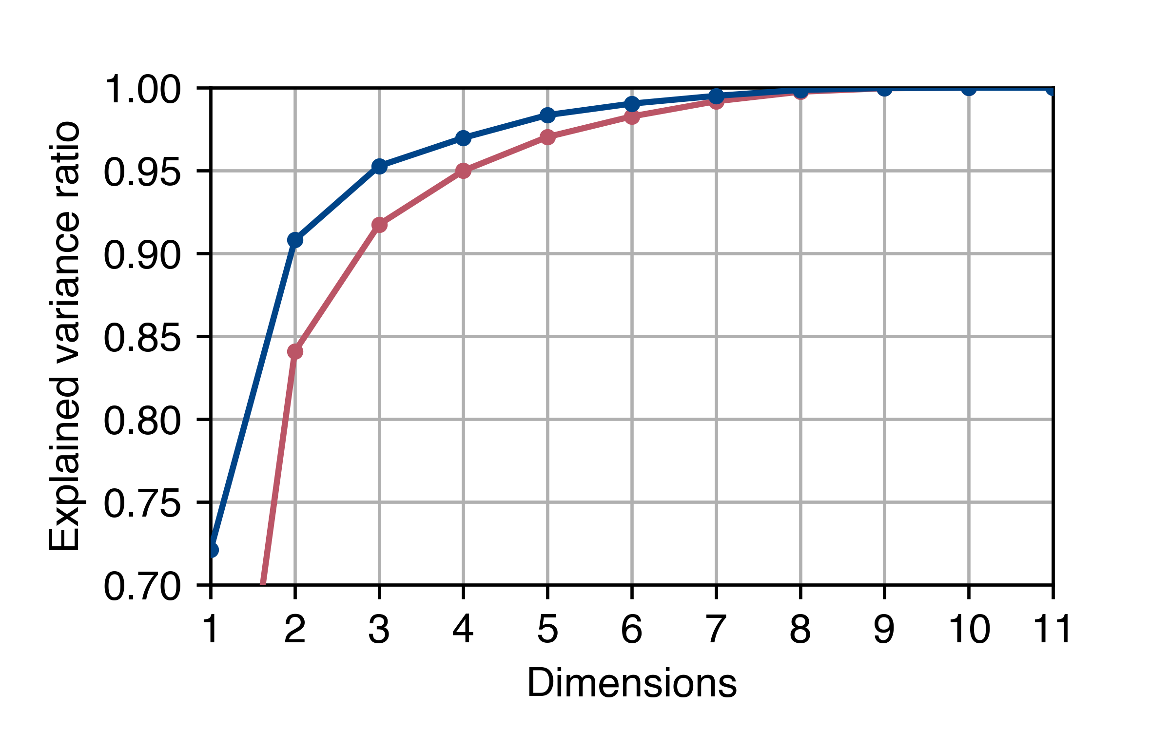
Machine learning requires data to train on. For this reason it is necessary to compile a database that we draw from both laboratory and commercial superalloys: with each entry encapsulating information for both the features that the ML method will take as inputs and also the properties that it will predict as outputs. In this work each row in the database is a different superalloy. The columns are the alloy’s descriptors comprising of composition (at. %), ageing heat treatment , and also its properties that are the components of both the alloy’s () and () phases and also the phase fraction . Since the composition must sum to one, a reduced description could be used. However principal component analysis (Fig. 1) showed that low rank projections of had more explanatory power than the same rank projections of (blue and red line respectively in Fig. 1). For this reason the full set of descriptors were used throughout. We focus on pure alloys and therefore circumvent consideration of any carbides and secondary phases that could form [2, 41, 42, 43, 44, 45, 46].
Heat treatments are applied to superalloys to control the microstructure morphology, and can be classed as either a solution heat treatment or a precipitation/ageing heat treatment. The solution heat treatment homogenises the microstructure so its temperature and duration is dictated by the superalloy composition [42, 47, 48]. Therefore, we consider the solution heat treatment as a property of the overall alloy composition, rather than as an input parameter. Next, ageing heat treatments are applied to further optimise the morphology of the superalloy microstructure. Six features describe the ageing heat treatment: a heat treatment temperature and time, for up to three heat treatment stages per alloy. For alloys with fewer total stages, the remaining ones are specified as being at room temperature for no time.
The database comprises 97 experimental superalloy microstructures, of which 36 entries correspond to laboratory alloys, 43 to commercial (or modifications of) single-crystal superalloys, and 18 to other commercial polycrystalline superalloys. All of these entries contained both Ni and Al. Other elements occurred in a subset of database entries, between 86-times for Cr to just 5-times for Ru [23, 40, 42, 48, 49, 50, 51, 52, 53, 54, 55, 56, 57, 58, 59, 60, 61, 62, 63, 64, 65, 66, 67, 68, 69, 70, 71, 72, 73, 74, 75, 76, 77, 78, 79, 80] . See Table 1 for a full overview including summary statistics. In order to make the training procedure as robust and user-friendly as possible, no outliers were filtered from the dataset before use in the ML model.
| Descriptors | ||||||||||||
| Phase composition (at. %) | ||||||||||||
| Ni | Cr | Co | Re | Ru | Al | Ta | W | Ti | Mo | Nb | Hf | |
| Min () | 47.28 | 3.00 | 2.50 | 0.64 | 1.30 | 2.00 | 0.44 | 0.03 | 1.12 | 0.31 | 0.006 | 0.03 |
| Max | 86.50 | 24.47 | 18.80 | 2.50 | 3.50 | 14.20 | 4.03 | 5.76 | 5.84 | 5.16 | 1.20 | 0.33 |
| Median | 66.50 | 12.55 | 6.65 | 2.00 | 3.50 | 11.20 | 1.99 | 1.53 | 2.70 | 1.30 | 0.44 | 0.06 |
| Mean | 67.46 | 12.30 | 8.20 | 1.75 | 3.06 | 9.89 | 1.97 | 1.83 | 2.88 | 1.97 | 0.39 | 0.13 |
| Frequency | 97 | 96 | 59 | 18 | 5 | 97 | 55 | 54 | 52 | 61 | 15 | 7 |
| Heat treatment (∘C hrs) | ||||||||||||
| #1 | #2 | #3 | ||||||||||
| Min () | 760 | 0.25 | 760 | 0.25 | 700 | 0.5 | ||||||
| Max | 1300 | 1500 | 1160 | 264 | 1050 | 100 | ||||||
| Median | 980 | 8 | 850 | 24 | 1040 | 16 | ||||||
| Mean | 963.8 | 305.2 | 856.9 | 31.0 | 941.4 | 24.8 | ||||||
| Frequency | 92 | 38 | 7 | |||||||||
| Properties | ||||||||||||
| log partitioning coefficient | ||||||||||||
| Ni | Cr | Co | Re | Ru | Al | Ta | W | Ti | Mo | Nb | ||
| Min | -0.692 | 0.404 | -0.208 | 0.142 | 1.169 | -6.984 | -5.711 | -0.411 | -5.220 | -0.463 | -1.872 | |
| Max | 0.133 | 3.086 | 1.665 | 7.078 | 1.508 | -0.488 | 0.489 | 1.329 | -0.340 | 2.006 | 1.454 | |
| Median | -0.154 | 2.038 | 1.077 | 1.794 | 1.218 | -1.500 | -1.892 | 0.311 | -1.740 | 1.239 | 0.022 | |
| Mean | -0.170 | 1.926 | 1.027 | 2.640 | 1.267 | -1.669 | -2.337 | 0.355 | -2.049 | 1.021 | -0.198 | |
| Frequency | 97 | 96 | 59 | 18 | 5 | 97 | 54 | 52 | 52 | 59 | 13 | |
| log partitioning coefficient | ||||||||||||
| Ni | Cr | Co | Re | Ru | Al | Ta | W | Ti | Mo | Nb | frac. | |
| Min | -0.297 | 0.274 | -0.037 | 0.122 | 0.390 | -1.410 | -1.208 | -0.446 | -1.293 | -0.405 | -0.795 | 0.030 |
| Max | 0.128 | 2.610 | 1.145 | 3.039 | 0.722 | 0.621 | 0.666 | 1.116 | -0.039 | 1.813 | 0.774 | 0.776 |
| Median | -0.058 | 1.320 | 0.508 | 0.857 | 0.568 | -0.445 | -0.356 | 0.100 | -0.423 | 0.594 | -0.432 | 0.470 |
| Mean | -0.063 | 1.361 | 0.550 | 1.194 | 0.565 | -0.518 | -0.371 | 0.173 | -0.550 | 0.643 | -0.136 | 0.450 |
| Frequency | 97 | 96 | 59 | 15 | 5 | 97 | 54 | 52 | 52 | 59 | 8 | 97 |
2.1 Data parameterisation
With the data curated we are now well-positioned to reparameterise it to both capture underlying physics and also to make it more amenable to machine learning. To express the phase composition we adopt logarithmic partitioning coefficients , [24, 23, 62, 63, 67, 73, 76]. They are defined as:
| (1) |
Predicting the logarithm of the partitioning coefficients ensures they always have physical positive values and preserves the symmetry between the and phases.
A superalloy comprises elements and phases, giving a total of variables of interest. The goal is to calculate them from the nominal composition of the superalloy . There are also the following physical constraints on these properties:
| (2) | ||||
| Total phases sum to unity. | (3) | |||
| (4) |
In our database entries is often determined from the measured chemical composition of each phase using the versions of Eq. 4, and is hence algebraically over-determined, resulting in an approximate value determined by finding the best fit for to a rearrangement of Eq. 4 [56, 81]. Typically this means Eq. 4 does not hold exactly. Another reason this equation may not be fulfilled exactly is that the phase fraction has been measured not only independently of the phase compositions but also via another method—e.g. via atom probe tomography or chemical analysis for the phase composition versus an ocular determination from SEM imagery for the phase fraction. In both cases Eq. 4 should hold to within the experimental tolerances of the independent and phase composition and fraction measurements.
Relaxing Eq. 4 from a strict constraint means that we need to predict all but one phase fraction, and for each phase all but one component, i.e. a total of predictions. In the subsequent sections we will refer to the specific case of superalloys, with phases. will refer to the fraction of or precipitate phase in the alloy, and can then be inferred by by Eq. 3. The constraints implied by Eq. 4 are revisited in section 3.2.
3 Computational method
3.1 Machine learning methodology
We adopt Gaussian process regression (GPR) machine learning to predict the log partitioning coefficients and and the phase fraction (and corresponding uncertainties) of each element in the alloy from its features. We can then calculate the final values for the microstructure to minimise the overall uncertainty. GPR takes a Bayesian approach to ML, in which an optimal posterior distribution—from which predictions are made—is formed from a prior distribution and a likelihood calculated from the training dataset. The prior distribution is assumed to be Gaussian with covariance determined by a kernel function. The functional form of the kernel should be chosen to suit the problem, but its hyperparameters are optimised using the training data. In this work we follow the standard approach of maximising the log marginal likelihood of the training data [82, 83]. The GPR implementation in the Scikit-learn library for Python was used [84].
Specifying the kernel provides an opportunity to incorporate our prior physical knowledge into the machine learning, which should give a more accurate model with less data. Superalloy properties are usually determined mainly by their composition rather than their heat treatment [52, 55, 57, 65, 68]. We capture this physical rule of thumb in the following kernel:
| (5) |
The first kernel term captures the bulk of the variation due to composition. The second kernel term captures the heat treatment and can be interpreted as an AND operation for the two measures of similarity, coupling heat treatment and composition [85]. A variation of Eq. 5 in which the second composition term was a constant was also tested.
Three alternate kernel functions were considered in this work. A simple and popular choice of kernel function is the Gaussian radial basis function (RBF):
| (6) |
Here is the norm. The kernel has a single hyperparameter to be optimised during fitting: the lengthscale . Our second choice is the linear kernel:
| (7) |
collapsing the method to ridge regression when [82, 85]. This was used as a comparison to the models with more complex kernels. The third choice is motivated by previous work that used GPR to model the effects of alloy heat treatments, which used the automatic relevance determination (ARD) variation on the Gaussian RBF kernel [86, 38]. This kernel introduces a length parameter for each feature, .
Often the phase behaviour of an alloy is governed by the concentrations of a few elements. This low dimensional structure can be encoded in the kernel by projecting the feature vector to a lower dimensional subspace, , with being a low rank matrix. could be found prior to fitting the kernel via principal component analysis, see Fig. 1, or it could be optimised as a hyperparameter of the kernel during training [87]. Prior knowledge tells us that we anticipate two main groups of elements in a superalloy—Ni-like elements, and Al-like elements—with a possible third group being the refractory elements [41, 43, 62, 63, 88], suggesting that a matrix of around rank 3 would be suitable.
3.1.1 Evaluating the quality of uncertainty prediction
GPR delivers uncertainty estimates for each of its predictions , so evaluating how close the uncertainties are to the real-life validation data, , is crucial. The typical error in a prediction should follow a Gaussian distribution with standard deviation . It follows that . This quantity is accumulated over all predictions and then is arranged into a histogram and compared to an ideal “Gaussian” histogram with bins of equal area such that each bin has equal noise. From this a distribution of uncertainty quality (DUQ) is defined as the absolute sum of the difference in the areas of bins between the two histograms. For data points this is defined as:
| (8) |
where the number of data points in each real bin, , is normalised such that . The number of bins is then optimised to achieve minimal value as described in the appendix. A minimal indicates a perfect estimate of the uncertainties whereas a peak indicates a poor estimate of uncertainty.
3.2 Calculation of phase compositions and fractions
3.2.1 Dynamic choice of balance element
For each component superalloy the relevant GPR models will predict all partitioning coefficients and the fraction, yielding compositions and also . This is more than the total number of properties needed, meaning for each phase the amount of one element, , will be calculated using Eq. 2—which we will call the balance element, . Rather than fixing one component to be the balance element in every alloy, we instead dynamically choose whichever minimises the difference between the component’s balance value and the GPR value, accounting for the uncertainty prediction of the GPR model , that is:
| (9) |
Since the numerator is the same for every element in a given alloy, this is equivalent to choosing the element with maximal uncertainty in its value to be the balance element.
For the final model presented in the next section, the dynamic choice of balance element was compared to a static choice, in this case the conventional choice of Ni. For Ni itself—a crucial element—the static method gave and in the and phases compared with an improvement of and respectively for the dynamic method. For Al there was also an improvement with the static method giving () and () compared with and for the dynamic method. This was despite Al being chosen as the balance element for 47 and 15 predictions (out of 97) for the and phase respectively using the dynamic method.
3.2.2 Bayesian inferral of a consistent precipitate fraction
Predicting the precipitate fraction , and the phase compositions and gives us a full determination of the microstructure. However the composition for each phase may not sum to the total composition—that is Eq. 4 will not hold exactly but it should hold approximately [56, 81]. To improve consistency a Bayesian approach was taken to synthesise the information from the output of the ML models for the phase compositions and for to give the phase composition most likely to be consistent with a valid total composition. The output of the GPR model for is taken as a prior, and the likelihood is taken to be:
With the standard deviation calculated from the uncertainties on the compositions as we have a conjugate prior to the likelihood and hence the posterior is also a Gaussian, with mean value and standard deviation:
| (10) | ||||
| (11) |
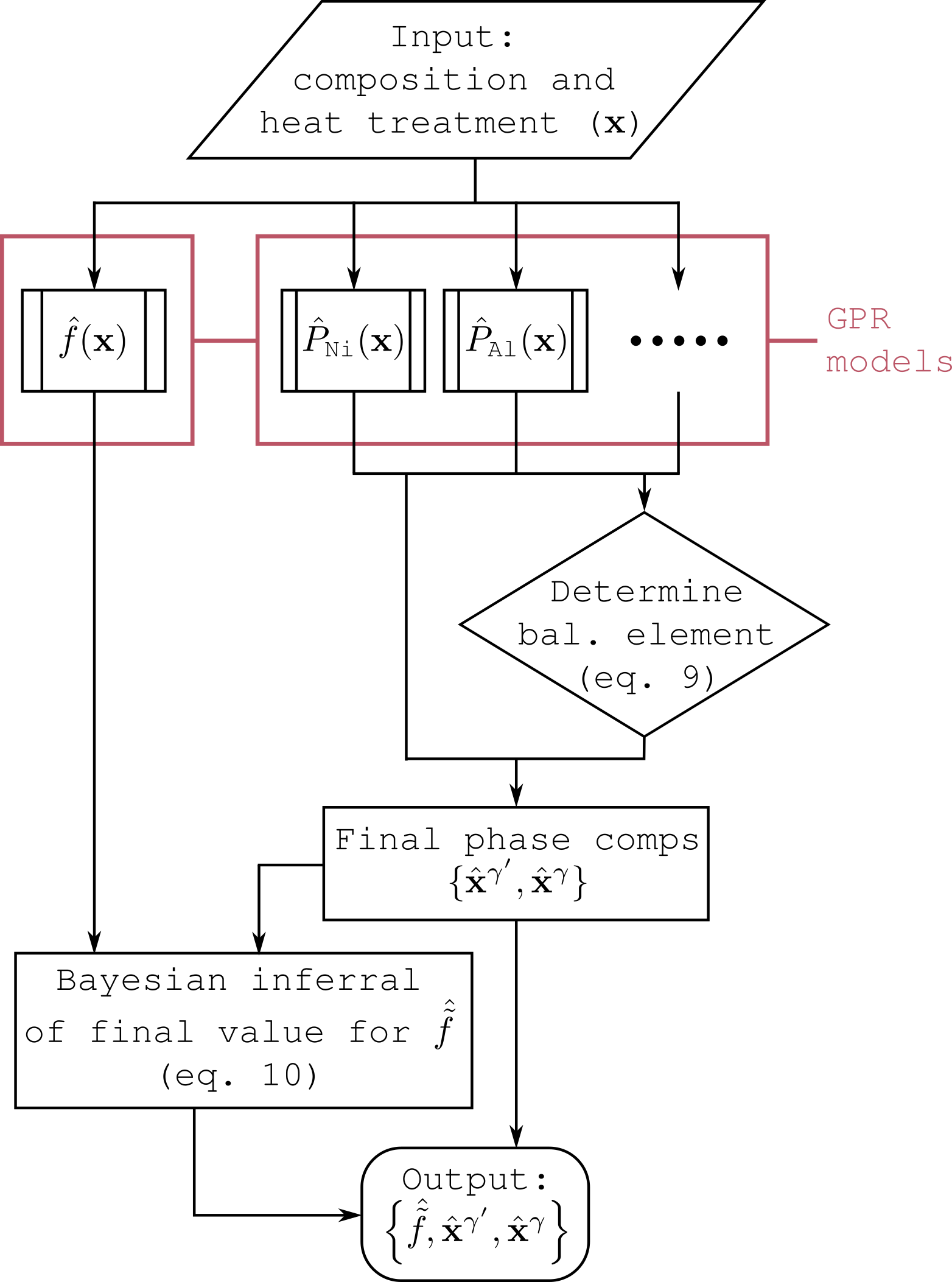
which are taken as the final values for the precipitate fraction and its uncertainty. Note that in the limit , Eq. 10 agrees with the method of Reed et al [56, 81]. The method described above can be viewed as transforming Eq. 4 from a strict constraint into a “soft” probabilistic constraint. A flowchart overview of how the final phase compositions and fractions are predicted for a given input composition is shown in Fig. 2.
4 Results and discussion
Variations of the GPR model with different kernels were trained on the database described in section 2. For each GPR model 5-fold cross validation was carried out. This procedure was used to fairly assess the quality of the different models in a way that will also highlight possible issues with over-fitting owing to a large number of variables. The step-by-step procedure is:
-
1.
80% of the initial dataset it selected at random as training data, with the remaining 20% being validation data.
- 2.
-
3.
The GPR model is tested against the validation data to get a measure of the accuracy. If the training data was over-fitted owing to a large number of model variables then the model will deliver poor accuracy against the blind validation data. Similarly, if the model has not captured the underlying physics of the dataset, it will perform comparatively poorly on the validation data.
-
4.
The procedure 1–3 is repeated five times with non-intersecting validation datasets so as to produce a validation prediction for all the data that is available, and the accuracy of each validation is stored.
-
5.
The accuracy of predictions on each of the five validation datasets are combined to deliver an overall coefficient of determination ( value) calculated over the entire dataset.
Throughout the following section the value calculated in this manner has been used as the metric to compare the different GPR models. We have also introduced the distribution of uncertainty quality (DUQ) described in section 3.1.1 as a metric to further explore the quality of a model’s predictions. Training on the full database took two minutes on a laptop with an Intel Core i7 CPU—once trained predictions can be made effectively instantaneously.
The Gaussian RBF (Eq. 6), linear (Eq. 7), and ARD kernels were initially tested for the composition only, . The results for selected properties are shown in Table 2. Using the linear kernel is broadly the same as the Alloy Design Program [23, 24, 25, 26, 27, 28], which gave good results for the fraction, but was less accurate for some elements in the phase. The RBF kernel gave slight improvements for Ni and Al in both phases as well as the fraction. The ARD kernel performed slightly worse than the standard RBF kernel overall, this is due to overfitting, as has been noted in previous work [89]. In the case of Gaussian RBF kernels, it was found overfitting could be reduced by setting the minimum value of the length scale to , corresponding to about half the phase diagram [85].
| Kernel | phase elements | phase elements | |||
|---|---|---|---|---|---|
| Ni | Al | Ni | Al | frac. | |
| Linear | 0.921 | 0.040 | 0.669 | 0.591 | 0.900 |
| RBF | 0.940 | 0.371 | 0.704 | 0.676 | 0.905 |
| ARD | 0.936 | 0.349 | 0.724 | 0.658 | 0.896 |
| Optimal (Eq. 12) | 0.927 | 0.599 | 0.824 | 0.674 | 0.917 |
With both linear and RBF kernels working well, a systematic approach was then taken to combining them according to the kernel scheme given in Eq. 5. The best results were found for the following kernel, henceforth referred to as the optimal kernel:
| (12) |
The first part is a linear kernel and the second an RBF kernel that combines composition and heat treatment, is a low rank matrix found from principal component analysis [85]. A projection onto the first 3 principal components was found to be optimal, in agreement with the discussion in section 3.1.
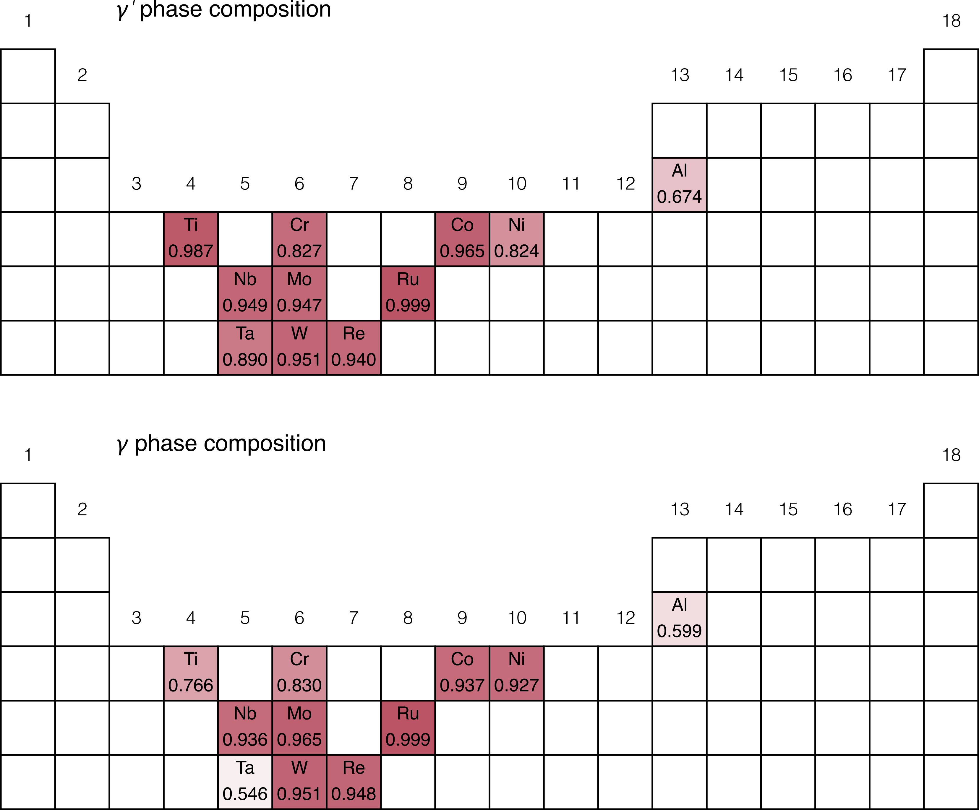
Kernel Eq. 12 gave excellent results for the fraction with , and for all components (the full set of values for this model are given in Fig. 5) except Al in the phase () and Al, Ta and Ti in the phase (, , respectively). This is due to the role of these three elements as formers. This role leads to their at. % in the phase being more constant between different alloys, resulting in a smaller variance and hence lower , most notably for Al. Analysis of the root mean-squared error (RMSE) showed it to be comparable to the other components. If Al, Ta, and Ti concentrations in the phase have a strong physical correlation to the alloy composition, this is not the case for the phase content—the remaining amount of each element that does not form the phase is dissolved into the phase—and for this reason it is less strongly correlated to the overall alloy composition which results in the generally lower values for the forming elements in the phase (Table 2).
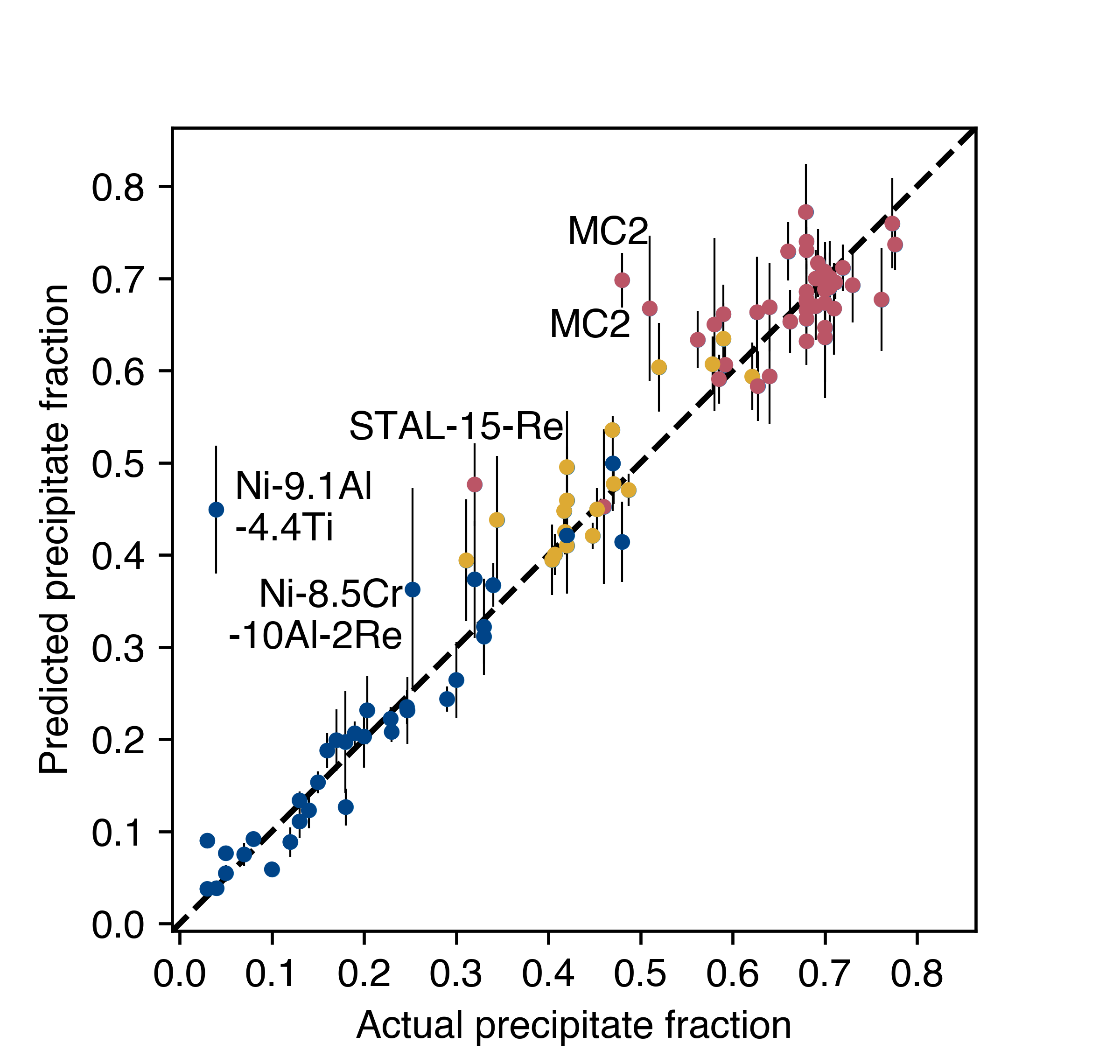
The predicted fractions found from this model are compared to the experimental values in Fig. 3. Agreement is on the whole excellent. The most significant outlier is lab alloy Ni-9.1Al-4.4Ti. This alloy is peculiar in having a low number of components with similar at. % values across both phase compositions and the nominal composition, which leads to a large error and uncertainty according to eqs. 10–11 [65]. Two other outliers are similar to training set alloys but with the addition of Re, suggesting more data for Re-bearing alloys may be required to explain its anomalous effect [56, 68]. Finally, two outliers correspond to the commercial single-crystal superalloy MC2 with extreme 3rd stage heat treatments (1050∘C for 10 hours and 100 hours respectively) [49]—again, more data is needed for extreme outlying heat treatment regimes, especially in the 3rd stage.
A variant of the optimal kernel Eq. 12 was also tested without the heat treatment term of the kernel which was set to 1. It performed similarly to the optimal kernel for phase composition predictions but was significantly outperformed for predictions of the phase fraction: it achieved an compared to for the optimal kernel. This tells us the optimal model is capturing the variance due to heat treatment, even if it is not capturing the full physics of complex heat treatment regimes such as the case of MC2 described above.
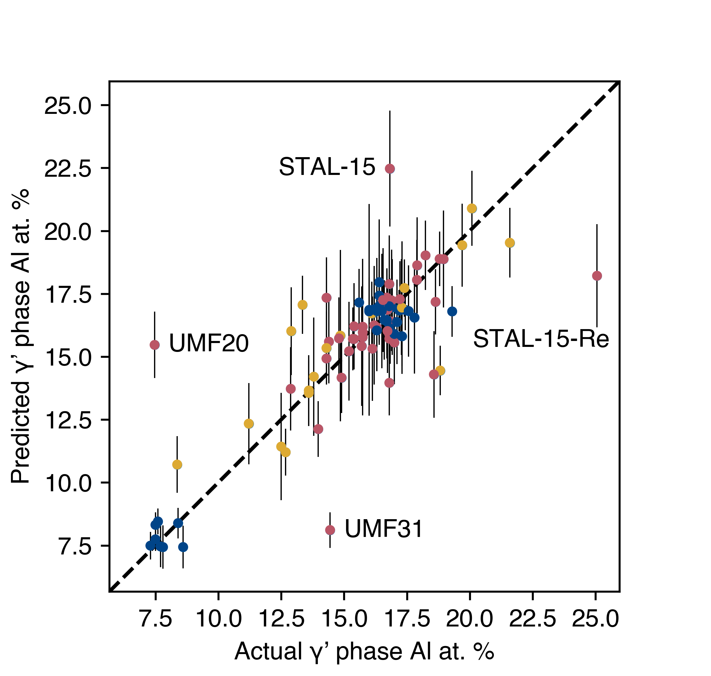
Fig. 4 shows the predictions for one crucial component—the Al content of the phase. Al is the principal former of the phase and the primary constituent of the secondary sublattice in this phase [41, 42]. Significant outliers are highlighted in the figure. Of these UMF20 and UMF31 are unusual compared to the other alloys because Ti rather than Al is the primary phase forming element in their composition [64, 73, 79]. In the case of STAL-15 and STAL-15-Re, they have similar input compositions whilst their reported phase compositions differ greatly hinting that they are either near to a phase transition or a possible anomalous result [56].
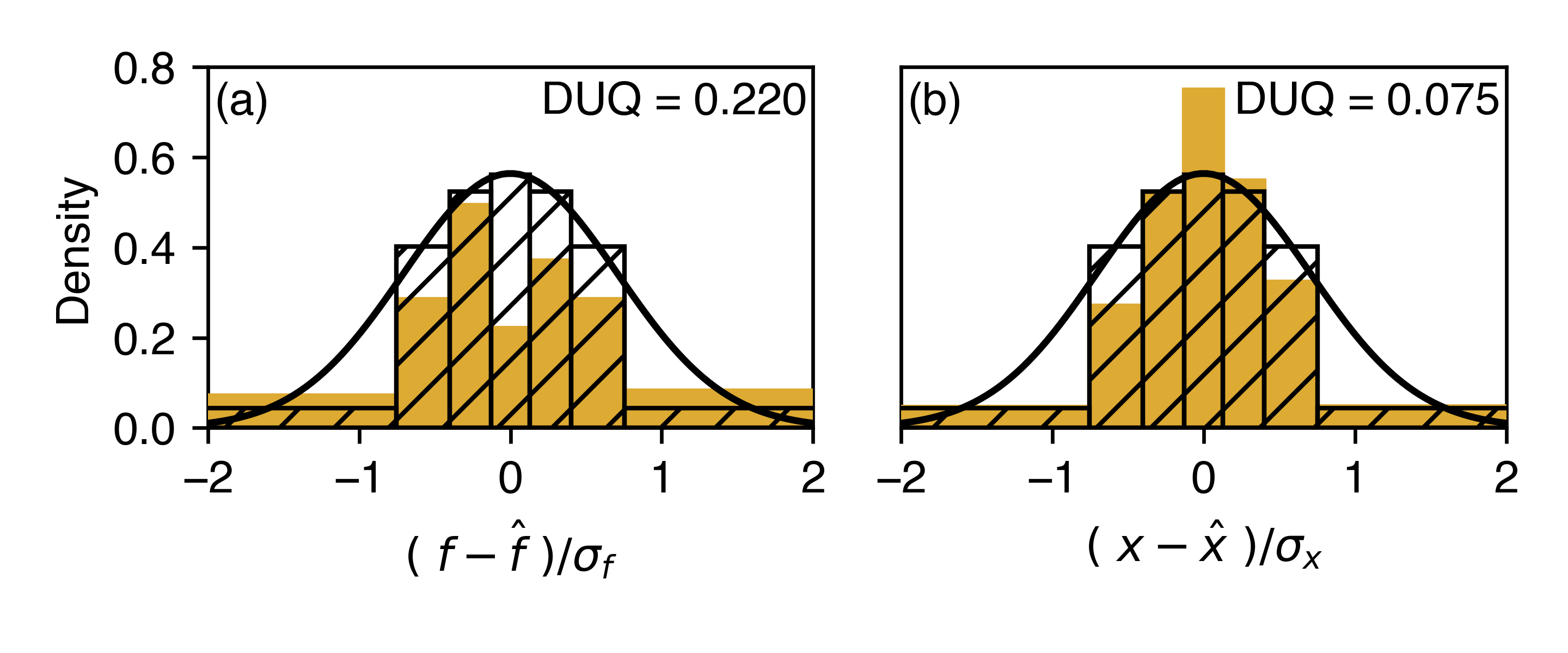
A key feature of GPR is the ability to estimate uncertainty in its predictions. Therefore, in Fig. 6 we compare the error in a prediction measured against the experimental value to the uncertainty in the prediction, which should take a single value. We study both the precipitate fraction and the chemical compositions. The area under each histogram in normalised to 1. For compositions the distribution is symmetrical and similar to the Gaussian distribution, with a comparatively small (see Eq. 8) . For the precipitate fraction the DUQ is larger at , and the distribution has a skew to under/overestimation.
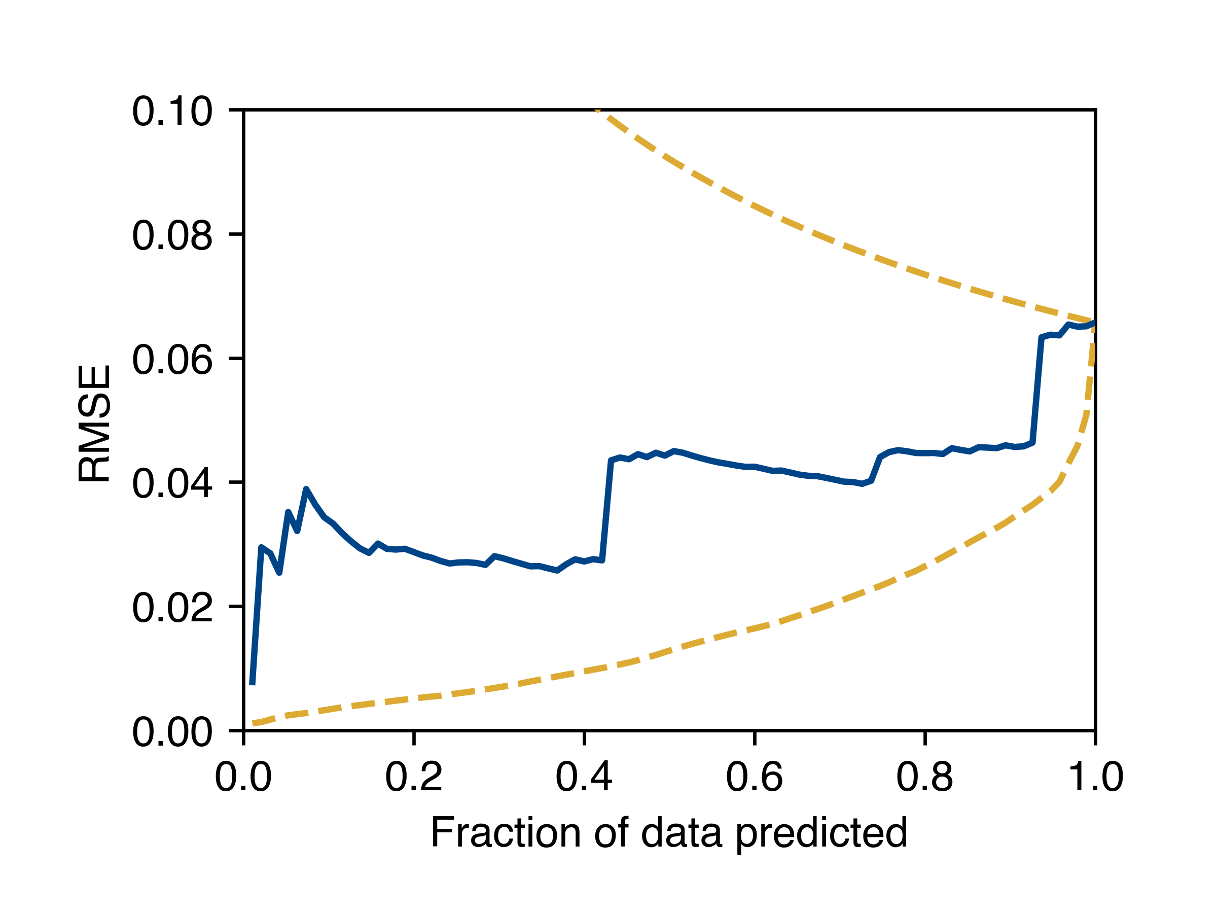
A practical advantage of having quantified uncertainties is that predictions can be filtered based on this uncertainty [90, 91]. Fig. 7 shows an example of this for the precipitate fraction. By focusing on only the most certain results, the RMSE reduces significantly, and is closer to the theoretical lower bound for the reduction than the upper bound. The lower and upper bound are given by filtering the data in the order that minimises or maximises respectively the RMSE. The steps in the blue curve in Fig. 7 occur as significant outlying predictions are filtered out. Each step corresponds to a significant outlier that can be identified on Fig. 3 by the magnitude of its uncertainty; for example the step at the highest fraction of data predicted corresponds to Ni-8.5Cr-10Al-2Re, the next MC2, then Ni-9.1Al-4.4Ti, etc. Step-like behaviour would vanish if all the predictions with the largest errors had the largest uncertainties, i.e. the lower bound curve in yellow. This method is useful when the model’s predictions are to be used to choose new alloy compositions for experimental testing, as it allows the alloy designer to only test compositions below a certain predicted error threshold and to focus on the predictions most likely to fulfil the target tolerance in an experiment.
4.1 Comparison to CALPHAD
The final GPR model was trained on the full database with 93 entries. It was then tested against unseen experimental atom probe tomography data collected by Sulzer et al for the SX-series alloys specifically for benchmarking the performance of CALPHAD [40] (data highlighted with an asterisk in B). In that test two thermodynamic databases were tested, TTNi8 and TCNi8 [16]. For each prediction tool, the root mean-squared error (RMSE) was calculated over all the elements in each phase in each SX-series alloy, as well as the precipitate fraction , giving three metrics for each method (Table 3). For both the and phases and the precipitate fraction , the GPR model is more accurate than CALPHAD.
| phase | phase | fraction | |
|---|---|---|---|
| Method | (RMSE) | (RMSE) | (RMSE) |
| TCNi8 | 0.0106 | 0.0354 | 0.0371 |
| TTNi8 | 0.0072 | 0.0324 | 0.0205 |
| This work | 0.0065 | 0.0321 | 0.0201 |
The composition of the SX series alloys in Ref. [40] had been chosen to explore a new region of composition space with high Cr content, and consequently both the GPR model and the two CALPHAD models were extrapolating in this region. Due to the inherent inclusion of physical laws it was anticipated that CALPHAD would be superior for extrapolative predictions, so it is particularly impressive that the GPR model outperforms CALPHAD. A further advantage of the GPR method is that it quantifies the uncertainty associated with predictions.
5 Conclusion
A Gaussian process regression model was developed to predict the compositional microstructure of nickel-base superalloys. It inputs the nominal composition of a superalloy and the ageing heat treatments, to then predict the chemical composition of the key and phases, and their relative abundance. The composition predictions are combined via a probabilistic approach to produce the final output composition. Cross-validation was used to compare a number of different kernel schemes for the GPR models, with the optimal kernel achieving a coefficient of determination for the precipitate fraction.
The real life utility of the GPR model was demonstrated by predicting the composition of the benchmark SX-series superalloys. The GPR model outperformed CALPHAD predictions using both the TTNi8 and TCNi8 databases [40]. This demonstrates the benefits of combining the best of physical and statistical approaches. The GPR model has a number of additional advantages over CALPHAD:
-
1.
Returns quantified uncertainty estimates for each prediction.
-
2.
No prior thermodynamic knowledge is required to construct the model.
-
3.
Model can easily be retrained as more data becomes available.
-
4.
Additional non-equilibrium effects can be incorporated in the model.
-
5.
Once trained, no free energy minimisation step is required to make predictions from the model.
-
6.
The trained model can be used to identify outliers in the initial dataset by highlighting property entries that lie the furthest from the model’s predictions [92].
As discussed above our GPR model made better predictions when the kernel included a heat treatment component, however further work is required to determine whether it can precisely capture the evolution of an alloy’s microstructure with different applied ageing heat treatments. Training and assessing the model on this problem is difficult due to the paucity of experimental data where phase composition has been determined for superalloys with the same nominal composition but different ageing heat treatments [49, 57]. A better representation of the heat treatment descriptors could improve this. Thermodynamic modelling approaches to predicting the effects of heat treatments do exist but their use in optimising heat treatments for alloys of pre-determined composition is involved [93, 94].
In this work we opted for the most straightforward dynamic method that makes use of the uncertainty in the initial predictions, Eq. 9. We found that this gave improved results for crucial elements such as Ni and Al compared to a fixed balance element model (Section 3.2.1). Alternate dynamic schemes for balancing the total phase composition in order to fulfil Eq. 2 can be devised, which may produce further improvements.
The GPR model is completely generic and can be applied to other material systems, meaning that it can be extended to predict other properties as well as thermodynamic ones. This would enable the development of a complete machine learning tool able to design practical alloys that simultaneously satisfy a range of target properties.
CRediT authorship contribution statement
Patrick Taylor: Conceptualisation, Methodology, Software, Formal analysis, Data curation, Writing—original draft. Gareth Conduit: Conceptualisation, Methodology, Writing—review & editing, Supervision.
Declaration of competing interest
Gareth Conduit is a Director of materials machine learning company Intellegens. The authors have no other financial interests or personal relationships that could have appeared to influence the work reported in this paper.
Acknowledgements
Patrick Taylor acknowledges the financial support of EPSRC and an ICASE award from Dassault Systèmes UK. Gareth Conduit acknowledges the financial support of the Royal Society. We would also like to thank Dr. Victor Milman and Dr. Alexander Perlov at Dassault Systèmes UK for their feedback on the manuscript. There is Open Access to this paper and data available at https://www.openaccess.cam.ac.uk/.
References
- [1] R. C. Reed, T. Tao, N. Warnken, Alloys-By-Design: Application to nickel-based single crystal superalloys, Acta Materialia 57 (19) (2009) 5898–5913. doi:10.1016/j.actamat.2009.08.018.
- [2] R. C. Reed, A. Mottura, D. J. Crudden, Alloys-By-Design: Towards Optimization of Compositions of Nickel-based Superalloys, in: Superalloys 2016, 2016, pp. 15–23.
- [3] M. Li, J. Coakley, D. Isheim, G. Tian, B. Shollock, Influence of the initial cooling rate from ’ supersolvus temperatures on microstructure and phase compositions in a nickel superalloy, Journal of Alloys and Compounds 732 (2018) 765–776. doi:10.1016/j.jallcom.2017.10.263.
- [4] A. van de Walle, G. Ceder, Automating first-principles phase diagram calculations, Journal of Phase Equilibria 23 (4) (2002) 348–359. doi:10.1361/105497102770331596.
- [5] A. van de Walle, Multicomponent multisublattice alloys, nonconfigurational entropy and other additions to the Alloy Theoretic Automated Toolkit, Calphad: Computer Coupling of Phase Diagrams and Thermochemistry 33 (2) (2009) 266–278. doi:10.1016/j.calphad.2008.12.005.
- [6] A. Van De Walle, P. Tiwary, M. De Jong, D. L. Olmsted, M. Asta, A. Dick, D. Shin, Y. Wang, L. Q. Chen, Z. K. Liu, Efficient stochastic generation of special quasirandom structures, Calphad: Computer Coupling of Phase Diagrams and Thermochemistry 42 (2013) 13–18. doi:10.1016/j.calphad.2013.06.006.
-
[7]
N. Schuch, F. Verstraete, Computational
complexity of interacting electrons and fundamental limitations of density
functionaltheory, Nature Physics 5 (10) (2009) 732–735.
doi:10.1038/nphys1370.
URL www.nature.com/naturephysics -
[8]
J. M. Sanchez,
Cluster
expansion and the configurational theory of alloys, Physical Review B -
Condensed Matter and Materials Physics 81 (22) (2010) 224202.
doi:10.1103/PhysRevB.81.224202.
URL https://journals.aps.org/prb/abstract/10.1103/PhysRevB.81.224202 -
[9]
A. Seko, Y. Koyama, I. Tanaka,
Cluster
expansion method for multicomponent systems based on optimal selection of
structures for density-functional theory calculations, Physical Review B -
Condensed Matter and Materials Physics 80 (16) (2009) 165122.
doi:10.1103/PhysRevB.80.165122.
URL https://journals.aps.org/prb/abstract/10.1103/PhysRevB.80.165122 -
[10]
I. S. Novikov, K. Gubaev, E. V. Podryabinkin, A. V. Shapeev,
The MLIP package: Moment
Tensor Potentials with MPI and Active Learning (7 2020).
doi:10.1088/2632-2153/abc9fe.
URL https://doi.org/10.1088/2632-2153/abc9fe - [11] K. Gubaev, Machine-Learning Interatomic Potentials for Multicomponent Alloys, Ph.D. thesis, Skoltech, Moscow (2018).
-
[12]
C. W. Rosenbrock, K. Gubaev, A. V. Shapeev, L. B. Pártay, N. Bernstein,
G. Csányi, G. L. Hart,
Machine-learned
interatomic potentials for alloys and alloy phase diagrams, npj
Computational Materials 7 (1) (2021) 1–9.
doi:10.1038/s41524-020-00477-2.
URL https://doi.org/10.1038/s41524-020-00477-2 -
[13]
V. L. Deringer, M. A. Caro, G. Csányi,
Machine
Learning Interatomic Potentials as Emerging Tools for Materials Science,
Advanced Materials 31 (46) (2019) 1902765.
doi:10.1002/adma.201902765.
URL https://onlinelibrary.wiley.com/doi/abs/10.1002/adma.201902765 - [14] M. C. Nguyen, L. Zhou, W. Tang, M. J. Kramer, I. E. Anderson, C. Z. Wang, K. M. Ho, Cluster-Expansion Model for Complex Quinary Alloys: Application to Alnico Permanent Magnets, Physical Review Applied 8 (5) (11 2017). doi:10.1103/PhysRevApplied.8.054016.
-
[15]
B. Grabowski, Y. Ikeda, P. Srinivasan, F. Körmann, C. Freysoldt, A. I.
Duff, A. Shapeev, J. Neugebauer,
Ab initio vibrational free
energies including anharmonicity for multicomponent alloys, npj
Computational Materials 5 (1) (2019) 1–6.
doi:10.1038/s41524-019-0218-8.
URL https://doi.org/10.1038/s41524-019-0218-8 - [16] J. O. Andersson, T. Helander, L. Höglund, P. Shi, B. Sundman, Thermo-Calc & DICTRA, computational tools for materials science, Calphad: Computer Coupling of Phase Diagrams and Thermochemistry 26 (2) (2002) 273–312. doi:10.1016/S0364-5916(02)00037-8.
-
[17]
B. Sundman, U. R. Kattner, M. Palumbo, S. G. Fries,
OpenCalphad
- a free thermodynamic software (12 2015).
doi:10.1186/s40192-014-0029-1.
URL https://link.springer.com/article/10.1186/s40192-014-0029-1 -
[18]
U. R. Kattner,
The CALPHAD
method and its role in material and process development, Tecnologia em
Metalurgia Materiais e Mineração 13 (1) (2016) 3–15.
doi:10.4322/2176-1523.1059.
URL http://tecnologiammm.com.br/doi/10.4322/2176-1523.1059 - [19] M. Hillert, Empirical methods of predicting and representing thermodynamic properties of ternary solution phases, Calphad 4 (1) (1980) 1–12. doi:10.1016/0364-5916(80)90016-4.
- [20] Y. A. Chang, S. Chen, F. Zhang, X. Yan, F. Xie, R. Schmid-Fetzer, W. A. Oates, Phase diagram calculation: Past, present and future, Progress in Materials Science 49 (3-4) (2004) 313–345. doi:10.1016/S0079-6425(03)00025-2.
- [21] S. Bajaj, A. Landa, P. Söderlind, P. E. Turchi, R. Arróyave, The U-Ti system: Strengths and weaknesses of the CALPHAD method, Journal of Nuclear Materials 419 (1-3) (2011) 177–185. doi:10.1016/j.jnucmat.2011.08.050.
- [22] V. Attari, P. Honarmandi, T. Duong, D. J. Sauceda, D. Allaire, R. Arroyave, Uncertainty propagation in a multiscale CALPHAD-reinforced elastochemical phase-field model, Acta Materialia 183 (2020) 452–470. doi:10.1016/j.actamat.2019.11.031.
- [23] H. Harada, K. Ohno, T. Yamagata, T. Yokokawa, M. Yamazaki, Phase calculation and its use in alloy design program for nickel-base superalloys, Tech. rep., Superalloys 1988 (1988).
-
[24]
H. Harada, H. Murakami,
Design of Ni-Base
Superalloys, in: T. Saito (Ed.), Computational Materials Design, Springer
Berlin Heidelberg, Berlin, Heidelberg, 1999, pp. 39–70.
doi:10.1007/978-3-662-03923-6{\_}2.
URL https://doi.org/10.1007/978-3-662-03923-6_2 - [25] K. Kawagishi, A.-C. Yeh, T. Yokokawa, T. Kobayashi, Y. Koizumi, H. Harada, Development of an Oxidation-Resistant High-Strength Sixth-Generation Single-Crystal Superalloy TMS-238, Tech. rep., Superalloys 2012: 12th International Symposium on Superalloys (2012).
- [26] A. Sato, H. Harada, A.-C. Yeh, K. Kawagishi, T. Kobayashi, Y. Koizumi, T. Yokokawa, J.-X. Zhang, A 5th generation SC superalloy with balanced high temperature properties and processability, Tech. rep., Superalloys 2008: 11th International Symposium on Superalloys (2008).
- [27] M. Enomoto, H. Harada, M. Yamazaki, Calculation of ’/ equilibrium phase compositions in nickel-base superalloys by cluster variation method, Calphad 15 (2) (1991) 143–158. doi:10.1016/0364-5916(91)90013-A.
- [28] Y. Saito, The Monte Carlo simulation of microstructural evolution in metals, Materials Science and Engineering A 223 (1-2) (1997) 114–124. doi:10.1016/s0921-5093(97)80019-6.
- [29] V. Venkatesh, H. J. Rack, Neural network approach to elevated temperature creep-fatigue life prediction, International Journal of Fatigue 21 (3) (1999) 225–234. doi:10.1016/S0142-1123(98)00071-1.
- [30] Y. S. Yoo, C. Y. Jo, C. N. Jones, Compositional prediction of creep rupture life of single crystal Ni base superalloy by Bayesian neural network, Materials Science and Engineering A 336 (1-2) (2002) 22–29. doi:10.1016/S0921-5093(01)01965-7.
-
[31]
F. Tancret, H. K. Bhadeshia, D. J. MacKay,
Design
of a creep resistant nickel base superalloy for power plant applications:
Part 1 - Mechanical properties modelling, Materials Science and Technology
19 (3) (2003) 283–290.
doi:10.1179/026708303225009788.
URL https://www.tandfonline.com/action/journalInformation?journalCode=ymst20 - [32] B. D. Conduit, N. G. Jones, H. J. Stone, G. J. Conduit, Design of a nickel-base superalloy using a neural network, Materials and Design 131 (2017) 358–365. doi:10.1016/j.matdes.2017.06.007.
- [33] B. D. Conduit, T. Illston, S. Baker, D. V. Duggappa, S. Harding, H. J. Stone, G. J. Conduit, Probabilistic neural network identification of an alloy for direct laser deposition, Materials and Design 168 (2019) 107644. doi:10.1016/j.matdes.2019.107644.
- [34] E. Menou, G. Ramstein, E. Bertrand, F. Tancret, Multi-objective constrained design of nickel-base superalloys using data mining- and thermodynamics-driven genetic algorithms, Modelling and Simulation in Materials Science and Engineering 24 (5) (4 2016). doi:10.1088/0965-0393/24/5/055001.
- [35] E. Menou, J. Rame, C. Desgranges, G. Ramstein, F. Tancret, Computational design of a single crystal nickel-based superalloy with improved specific creep endurance at high temperature, Computational Materials Science 170 (2019) 109194. doi:10.1016/j.commatsci.2019.109194.
- [36] Y. Liu, J. Wu, Z. Wang, X. G. Lu, M. Avdeev, S. Shi, C. Wang, T. Yu, Predicting creep rupture life of Ni-based single crystal superalloys using divide-and-conquer approach based machine learning, Acta Materialia 195 (2020) 454–467. doi:10.1016/j.actamat.2020.05.001.
-
[37]
Y. Zhang, X. Xu, Lattice
Misfit Predictions via the Gaussian Process Regression for Ni-Based Single
Crystal Superalloys, Metals and Materials International (2020) 1–19doi:10.1007/s12540-020-00883-7.
URL https://doi.org/10.1007/s12540-020-00883-7 - [38] Y. C. Yabansu, A. Iskakov, A. Kapustina, S. Rajagopalan, S. R. Kalidindi, Application of Gaussian process regression models for capturing the evolution of microstructure statistics in aging of nickel-based superalloys, Acta Materialia 178 (2019) 45–58. doi:10.1016/j.actamat.2019.07.048.
- [39] Y. Yuan, K. Kawagishi, Y. Koizumi, T. Kobayashi, T. Yokokawa, H. Harada, Creep deformation of a sixth generation Ni-base single crystal superalloy at 800∘C, Materials Science and Engineering A 608 (2014) 95–100. doi:10.1016/j.msea.2014.04.069.
-
[40]
S. Sulzer, M. Hasselqvist, H. Murakami, P. Bagot, M. Moody, R. Reed,
The Effects of Chemistry
Variations in New Nickel-Based Superalloys for Industrial Gas Turbine
Applications, Metallurgical and Materials Transactions A: Physical
Metallurgy and Materials Science 51 (9) (2020) 4902–4921.
doi:10.1007/s11661-020-05845-7.
URL https://doi.org/10.1007/s11661-020-05845-7 - [41] R. C. Reed, The superalloys fundamentals and applications, Cambridge University Press, Cambridge, UK ; New York, 2006.
- [42] M. Durand-Charre, The microstructure of superalloys, CRC Press, Boca Raton, Fl, USA, 1997.
- [43] W. Z. Wang, T. Jin, J. L. Liu, X. F. Sun, H. R. Guan, Z. Q. Hu, Role of Re and Co on microstructures and ’ coarsening in single crystal superalloys, Materials Science and Engineering A 479 (1-2) (2008) 148–156. doi:10.1016/j.msea.2007.06.031.
- [44] L. Zhang, Z. Huang, Y. Pan, L. Jiang, Design of Re-free nickel-base single crystal superalloys using modelling and experimental validations, Modelling and Simulation in Materials Science and Engineering 27 (6) (5 2019). doi:10.1088/1361-651X/ab2031.
- [45] M. Pröbstle, S. Neumeier, P. Feldner, R. Rettig, H. E. Helmer, R. F. Singer, M. Göken, Improved creep strength of nickel-base superalloys by optimized /’ partitioning behavior of solid solution strengthening elements, Materials Science and Engineering A 676 (2016). doi:10.1016/j.msea.2016.08.121.
- [46] R. A. Hobbs, L. Zhang, C. M. Rae, S. Tin, The effect of ruthenium on the intermediate to high temperature creep response of high refractory content single crystal nickel-base superalloys, Materials Science and Engineering A 489 (1-2) (2008) 65–76. doi:10.1016/j.msea.2007.12.045.
- [47] P. Caron, C. Ramusat, F. Diologent, Influence of the ’ fraction on the /’ topological inversion during high temperature creep of single crystal superalloys, Tech. rep., Superalloys 2008: 11th International Symposium on Superalloys (2008).
- [48] T. Khan, P. Caron, C. Duret, The development and characterization of a high performance experimental single crystal superalloy, in: Superalloys 1984, Superalloys 1984, 1984, pp. 145–155.
- [49] S. Duval, S. Chambreland, P. Caron, D. Blavette, Phase composition and chemical order in the single crystal nickel base superalloy MC2, Acta Metallurgica Et Materialia (1994). doi:10.1016/0956-7151(94)90061-2.
- [50] R. Glas, M. Jouiad, P. Caron, N. Clement, H. O. Kirchner, Order and mechanical properties of the matrix of superalloys, Acta Materialia (1996). doi:10.1016/S1359-6454(96)00096-1.
- [51] H. Harada, A. Ishida, Y. Murakami, H. K. Bhadeshia, M. Yamazaki, Atom-probe microanalysis of a nickel-base single crystal superalloy, Applied Surface Science 67 (1-4) (1993) 299–304. doi:10.1016/0169-4332(93)90329-A.
- [52] T. Khan, P. Caron, Effect of processing conditions and heat treatments on mechanical properties of single-crystal superalloy CMSX-2, Materials Science and Technology (United Kingdom) 2 (5) (1986) 486–492. doi:10.1179/mst.1986.2.5.486.
- [53] M. K. Miller, R. Jayaram, L. S. Lin, A. D. Cetel, APFIM characterization of single-crystal PWA 1480 nickel-base superalloy, Applied Surface Science 76-77 (C) (1994) 172–176. doi:10.1016/0169-4332(94)90339-5.
- [54] A. Royer, P. Bastie, M. Veron, In situ determination of ’ phase volume fraction and of relations between lattice parameters and precipitate morphology in ni-based single crystal superalloy, Acta Materialia 46 (15) (1998) 5357–5368. doi:10.1016/S1359-6454(98)00206-7.
- [55] F. Diologent, P. Caron, On the creep behavior at 1033 K of new generation single-crystal superalloys, Materials Science and Engineering A 385 (1-2) (2004) 245–257. doi:10.1016/j.msea.2004.07.016.
- [56] M. Segersäll, P. Kontis, S. Pedrazzini, P. A. Bagot, M. P. Moody, J. J. Moverare, R. C. Reed, Thermal-mechanical fatigue behaviour of a new single crystal superalloy: Effects of Si and Re alloying, Acta Materialia 95 (2015) 456–467. doi:10.1016/j.actamat.2015.03.060.
- [57] R. Schmidt, M. Feller-Kniepmeier, Effect of heat treatments on phase chemistry of the Nickel-Base superalloy SRR 99, Metallurgical Transactions A 23 (3) (1992) 745–757. doi:10.1007/BF02675552.
- [58] M. V. Nathal, L. J. Ebert, Elevated temperature creep-rupture behavior of the single crystal nickel-base superalloy NASAIR 100, Metallurgical Transactions A 16 (3) (1985) 427–439. doi:10.1007/BF02814341.
- [59] W. T. Loomis, J. W. Freeman, D. L. Sponseller, The influence of molybdenum on the /’phase in experimental nickel-base superalloys, Metallurgical and Materials Transactions B 3 (4) (1972) 989–1000. doi:10.1007/bf02647677.
- [60] H. Morrow, D. L. Sponseller, M. Semchyshen, The effects of molybdenum and aluminum on the thermal expansion coefficients of nickel-base alloys, Metallurgical Transactions A 6 (2) (1975) 477–485. doi:10.1007/BF02658405.
- [61] F. Pettinari, J. Douin, G. Saada, P. Caron, A. Coujou, N. Clément, Stacking fault energy in short-range ordered -phases of Ni-based superalloys, Materials Science and Engineering A (2002). doi:10.1016/S0921-5093(01)01765-8.
- [62] A. P. Ofori, C. J. Humphreys, S. Tin, C. N. Jones, A TEM study of the effect of platinum group metals in advanced single crystal nickel-base superalloys, Tech. rep., Superalloys 2004: 10th International Symposium on Superalloys (2004).
- [63] S. Tin, A. C. Yeh, A. P. Ofori, R. C. Reed, S. S. Babu, M. K. Miller, Atomic partitioning of ruthenium in Ni-based superalloys, Tech. rep., Superalloys 2004: 10th International Symposium on Superalloys (2004).
- [64] K. M. Delargy, G. D. Smith, Phase composition and phase stability of high-chromium nickel-based superalloy, IN939, Metallurgical transactions. A, Physical metallurgy and materials science 14 A (9) (1983) 1771–1783. doi:10.1007/BF02645547.
- [65] B. Ralph, S. A. Hill, M. J. Southon, M. P. Thomas, A. R. Waugh, The investigation of engineering materials using atom-probe techniques, Ultramicroscopy 8 (3) (1982) 361–375. doi:10.1016/0304-3991(82)90254-6.
- [66] D. Blavette, P. Duval, L. Letellier, M. Guttmann, Atomic-scale APFIM and TEM investigation of grain boundary microchemistry in astroloy nickel base superalloys, Acta Materialia 44 (12) (1996) 4995–5005. doi:10.1016/S1359-6454(96)00087-0.
- [67] G. E. Fuchs, B. A. Boutwell, Modeling of the partitioning and phase transformation temperatures of an as-cast third generation single crystal Ni-base superalloy, Materials Science and Engineering A 333 (1-2) (2002) 72–79. doi:10.1016/S0921-5093(01)01825-1.
- [68] K. E. Yoon, R. D. Noebe, D. N. Seidman, Effects of rhenium addition on the temporal evolution of the nanostructure and chemistry of a model Ni-Cr-Al superalloy. I: Experimental observations, Acta Materialia 55 (4) (2007) 1145–1157. doi:10.1016/j.actamat.2006.08.027.
-
[69]
A. B. Parsa, P. Wollgramm, H. Buck, C. Somsen, A. Kostka, I. Povstugar, P.-P.
Choi, D. Raabe, A. Dlouhy, J. Müller, E. Spiecker, K. Demtroder,
J. Schreuer, K. Neuking, G. Eggeler,
Advanced Scale Bridging
Microstructure Analysis of Single Crystal Ni-Base Superalloys, Advanced
Engineering Materials 17 (2) (2015) 216–230.
doi:10.1002/adem.201400136.
URL http://doi.wiley.com/10.1002/adem.201400136 - [70] D. Siebörger, H. Knake, U. Glatzel, Temperature dependence of the elastic moduli of the nickel-base superalloy CMSX-4 and its isolated phases, Materials Science and Engineering A 298 (1-2) (2001) 26–33. doi:10.1016/s0921-5093(00)01318-6.
- [71] M. Fahrmann, W. Hermann, E. Fahrmann, A. Boegli, T. M. Pollock, H. G. Sockel, Determination of matrix and precipitate elastic constants in (-’) Ni-base model alloys, and their relevance to rafting, Materials Science and Engineering A 260 (1-2) (1999) 212–221. doi:10.1016/s0921-5093(98)00953-8.
- [72] Y. Yuan, Y. Gu, C. Cui, T. Osada, Z. Zhong, T. Tetsui, T. Yokokawa, H. Harada, Influence of Co content on stacking fault energy in Ni-Co base disk superalloys, Journal of Materials Research 26 (22) (2011) 2833–2837. doi:10.1557/jmr.2011.346.
- [73] S. Ma, L. Carroll, T. M. Pollock, Development of phase stacking faults during high temperature creep of Ru-containing single crystal superalloys, Acta Materialia 55 (17) (2007) 5802–5812. doi:10.1016/j.actamat.2007.06.042.
- [74] C. Y. Cui, C. G. Tian, Y. Z. Zhou, T. Jin, X. F. Sun, Dynamic strain aging in Ni base alloys with different stacking fault energy, Tech. rep., Superalloys 2012: 12th International Symposium on Superalloys (2012).
- [75] M. T. Jovanović, Z. Miškovic, B. Lukić, Microstructure and stress-rupture life of polycrystal, directionally solidified, and single crystal castings of nickel-based IN 939 superalloy, Materials Characterization 40 (4-5) (1998) 261–268. doi:10.1016/s1044-5803(98)00013-8.
- [76] X. G. Wang, J. L. Liu, T. Jin, X. F. Sun, The effects of ruthenium additions on tensile deformation mechanisms of single crystal superalloys at different temperatures, Materials and Design 63 (2014) 286–293. doi:10.1016/j.matdes.2014.06.009.
-
[77]
J. P. Collier,
Effects of
replacing the refractory elements W, Nb and Ta with Mo in nickel-bases
superalloys on microstructural, microchemistry, and mechanical properties.,
Metallurgical transactions. A, Physical metallurgy and materials science 17
A (4) (1986) 651–661.
doi:10.1007/BF02643984.
URL https://link.springer.com/article/10.1007/BF02643984 - [78] H. Long, S. Mao, Y. Liu, Z. Zhang, X. Han, Microstructural and compositional design of Ni-based single crystalline superalloys ― A review (4 2018). doi:10.1016/j.jallcom.2018.01.224.
- [79] S. T. Wlodek, M. Kelly, D. A. Alden, The Structure of Rene 88 DT, Tech. rep., Superalloys 1996 (1996).
-
[80]
M. T. Lapington, D. J. Crudden, R. C. Reed, M. P. Moody, P. A. Bagot,
Characterization of Phase
Chemistry and Partitioning in a Family of High-Strength Nickel-Based
Superalloys, Metallurgical and Materials Transactions A: Physical
Metallurgy and Materials Science 49 (6) (2018) 2302–2310.
doi:10.1007/s11661-018-4558-7.
URL https://doi.org/10.1007/s11661-018-4558-7 - [81] R. C. Reed, A. C. Yeh, S. Tin, S. S. Babu, M. K. Miller, Identification of the partitioning characteristics of ruthenium in single crystal superalloys using atom probe tomography, Scripta Materialia 51 (4) (2004) 327–331. doi:10.1016/j.scriptamat.2004.04.019.
- [82] C. E. Rasmussen, C. K. Williams, Gaussian processes for machine learning, Adaptive computation and machine learning, MIT Press, Cambridge, Mass., 2006.
-
[83]
M. Kanagawa, P. Hennig, D. Sejdinovic, B. K. Sriperumbudur,
Gaussian Processes and Kernel
Methods: A Review on Connections and Equivalences, arXiv (7 2018).
URL http://arxiv.org/abs/1807.02582 -
[84]
F. Pedregosa, G. Varoquaux, A. Gramfort, V. Michel, B. Thirion, O. Grisel,
M. Blondel, P. Prettenhofer, R. Weiss, V. Dubourg, J. Vanderplas, A. Passos,
D. Cournapeau, M. Brucher, M. Perrot, E. Duchesnay,
Scikit-learn: Machine learning in Python,
Journal of Machine Learning Research 12 (2011) 2825–2830.
URL http://scikit-learn.org. - [85] D. K. Duvenaud, Automatic model construction with Gaussian processes, Ph.D. thesis, University of Cambridge, Cambridge (2014).
- [86] R. Tamura, T. Osada, K. Minagawa, T. Kohata, M. Hirosawa, K. Tsuda, K. Kawagishi, Machine learning-driven optimization in powder manufacturing of Ni-Co based superalloy, Materials and Design 198 (2021) 109290. doi:10.1016/j.matdes.2020.109290.
-
[87]
E. Snelson, Z. Ghahramani, Variable
noise and dimensionality reduction for sparse Gaussian processes,
Proceedings of the 22nd Conference on Uncertainty in Artificial Intelligence,
UAI 2006 (2012) 461–468.
URL http://arxiv.org/abs/1206.6873 -
[88]
T. M. Pollock, S. Tin, Nickel-based superalloys for
advanced turbine engines: Chemistry, microstructure, and properties (5
2006).
doi:10.2514/1.18239.
URL http://arc.aiaa.org -
[89]
R. O. Mohammed, G. C. Cawley,
Over-fitting in model selection with
Gaussian process regression, in: Lecture Notes in Computer Science
(including subseries Lecture Notes in Artificial Intelligence and Lecture
Notes in Bioinformatics), Vol. 10358 LNAI, Springer Verlag, 2017, pp.
192–205.
doi:10.1007/978-3-319-62416-7{\_}14.
URL http://theoval.cmp.uea.ac.uk/ - [90] E. J. Martin, V. R. Polyakov, L. Tian, R. C. Perez, Profile-QSAR 2.0: Kinase Virtual Screening Accuracy Comparable to Four-Concentration IC50s for Realistically Novel Compounds, Journal of Chemical Information and Modeling 57 (8) (2017) 2077–2088. doi:10.1021/acs.jcim.7b00166.
-
[91]
B. W. Irwin, J. R. Levell, T. M. Whitehead, M. D. Segall, G. J. Conduit,
Practical
Applications of Deep Learning to Impute Heterogeneous Drug Discovery Data,
Journal of Chemical Information and Modeling 60 (6) (2020) 2848–2857.
doi:10.1021/acs.jcim.0c00443.
URL https://pubs.acs.org/doi/abs/10.1021/acs.jcim.0c00443 - [92] P. C. Verpoort, P. MacDonald, G. J. Conduit, Materials data validation and imputation with an artificial neural network, Computational Materials Science 147 (2018) 176–185. doi:10.1016/J.COMMATSCI.2018.02.002.
- [93] D. M. Collins, B. D. Conduit, H. J. Stone, M. C. Hardy, G. J. Conduit, R. J. Mitchell, Grain growth behaviour during near-’ solvus thermal exposures in a polycrystalline nickel-base superalloy, Acta Materialia 61 (9) (2013) 3378–3391. doi:10.1016/J.ACTAMAT.2013.02.028.
- [94] D. M. Collins, H. J. Stone, A modelling approach to yield strength optimisation in a nickel-base superalloy, International Journal of Plasticity 54 (2014) 96–112. doi:10.1016/J.IJPLAS.2013.08.009.
- [95] V. Jalilvand, H. Omidvar, M. R. Rahimipour, H. R. Shakeri, Influence of bonding variables on transient liquid phase bonding behavior of nickel based superalloy IN-738LC, Materials and Design 52 (2013) 36–46. doi:10.1016/j.matdes.2013.05.042.
- [96] A. Basak, S. Das, Microstructure of nickel-base superalloy MAR-M247 additively manufactured through scanning laser epitaxy (SLE), Journal of Alloys and Compounds 705 (2017) 806–816. doi:10.1016/j.jallcom.2017.02.013.
- [97] D. Blavette, P. Caron, T. Khan, An atom probe investigation of the role of rhenium additions in improving creep resistance of Ni-base superalloys, Scripta Metallurgica 20 (10) (1986) 1395–1400. doi:10.1016/0036-9748(86)90103-1.
- [98] R. C. Reed, A. C. Yeh, S. Tin, S. S. Babu, M. K. Miller, Identification of the partitioning characteristics of ruthenium in single crystal superalloys using atom probe tomography, Scripta Materialia 51 (4) (2004) 327–331. doi:10.1016/j.scriptamat.2004.04.019.
Appendix A Distribution of uncertainty quality
The distribution of uncertainty quality (DUQ) as defined in Eq. 8 has a minimum value of 0 and a maximum value of 1 which can be seen by considering the norm on the vectors . For both the ideal and real histogram the edges of each bin are defined such that:
| (A1) |
where is the PDF for the Gaussian distribution , and the area of each ideal bin is . This ensures the histogram for the ideal distribution has a total area of 1. For an odd number of bins the rightmost edges with are given by:
| (A2) |
where .
The number of bins is optimised by minimising a quantity related to the DUQ:
| (A3) |
where is the height of the ideal bin at position . The second term accounts for the difference in area between the ideal bins and the normal distribution, which favours larger numbers of bins. Minimising the DUQ directly will always lead to the minimum number of bins being used.
Eq. A2 leads to the outermost bins having infinite width and zero height. For visualisation purposes this is undesirable so a cutoff can be introduced that gives all the bins finite width whilst not affecting the optimal number of bins. We found a cutoff to be a suitable choice.
Appendix B Database of alloys
The full database of alloys as described in section 2. The SX-series alloys have been highlighted in each table with an asterisk.
| # | Ref. | Composition at. % | |||||||||||
| Ni | Cr | Co | Re | Ru | Al | Ta | W | Ti | Mo | Nb | Hf | ||
| 1 | [49] | 65.90 | 9.30 | 5.10 | - | - | 11.20 | 2.00 | 2.60 | 2.50 | 1.30 | - | - |
| 2 | [49] | 65.90 | 9.30 | 5.10 | - | - | 11.20 | 2.00 | 2.60 | 2.50 | 1.30 | - | - |
| 3 | [49] | 65.90 | 9.30 | 5.10 | - | - | 11.20 | 2.00 | 2.60 | 2.50 | 1.30 | - | - |
| 4 | [49] | 65.90 | 9.30 | 5.10 | - | - | 11.20 | 2.00 | 2.60 | 2.50 | 1.30 | - | - |
| 5 | [50] | 66.50 | 8.87 | 5.38 | - | - | 12.81 | 1.11 | 1.56 | 2.41 | 1.35 | - | - |
| 6 | [51] | 72.00 | 7.80 | - | - | - | 12.70 | 2.80 | - | - | 4.60 | - | - |
| 7 | [23] | 65.30 | 6.75 | 8.12 | - | - | 12.29 | 1.80 | 5.76 | - | - | - | - |
| 8 | [23] | 64.66 | 11.68 | 5.15 | - | - | 11.25 | 4.03 | 1.32 | 1.90 | - | - | - |
| 9 | [23] | 66.29 | 9.22 | 5.09 | - | - | 13.55 | 1.99 | 2.61 | - | 1.25 | - | - |
| 10 | [23, 95] | 59.89 | 17.67 | 8.23 | - | - | 7.19 | 0.54 | 0.81 | 4.05 | 1.07 | 0.55 | - |
| 11 | [23, 77] | 62.81 | 9.19 | 9.72 | - | - | 12.33 | 1.25 | 0.03 | 1.15 | 3.51 | 0.01 | - |
| 12 | [23, 96] | 61.22 | 9.17 | 10.11 | - | - | 13.25 | 0.99 | 3.24 | 1.24 | 0.43 | - | 0.33 |
| 13 | [23] | 67.77 | 9.19 | 4.66 | - | - | 12.40 | 1.91 | 2.57 | 1.12 | 0.37 | - | - |
| 14 | [52] | 67.77 | 9.19 | 4.66 | - | - | 12.40 | 1.91 | 2.57 | 1.12 | 0.37 | - | - |
| 15 | [52] | 67.77 | 9.19 | 4.66 | - | - | 12.40 | 1.91 | 2.57 | 1.12 | 0.37 | - | - |
| 16 | [48] | 71.38 | 9.22 | - | - | - | 13.55 | 1.99 | 2.61 | - | 1.25 | - | - |
| 17 | [48] | 66.29 | 9.22 | 5.09 | - | - | 13.55 | 1.99 | 2.61 | - | 1.25 | - | - |
| 18 | [48] | 63.74 | 9.22 | 7.63 | - | - | 13.56 | 1.99 | 2.61 | - | 1.25 | - | - |
| 19 | [53] | 65.10 | 11.50 | 5.10 | - | - | 11.00 | 4.00 | 1.40 | 1.90 | - | - | - |
| 20 | [53] | 65.10 | 11.50 | 5.10 | - | - | 11.00 | 4.00 | 1.40 | 1.90 | - | - | - |
| 21 | [54] | 65.60 | 8.70 | 6.60 | - | - | 11.80 | 2.70 | 1.80 | 1.50 | 1.30 | - | - |
| 22 | [55] | 65.54 | 9.04 | 6.65 | - | - | 11.62 | 2.63 | 1.87 | 1.39 | 1.26 | - | - |
| 23 | [55] | 65.54 | 9.04 | 6.65 | - | - | 11.62 | 2.63 | 1.87 | 1.39 | 1.26 | - | - |
| 24 | [55] | 65.54 | 9.04 | 6.65 | - | - | 11.62 | 2.63 | 1.87 | 1.39 | 1.26 | - | - |
| 25 | [56] | 62.85 | 17.74 | 5.06 | - | - | 9.94 | 2.56 | 1.23 | - | 0.62 | - | 0.03 |
| 26 | [56] | 62.52 | 17.81 | 5.06 | 0.64 | - | 10.03 | 2.64 | 0.65 | - | 0.61 | - | 0.04 |
| 27 | [57] | 66.70 | 9.60 | 5.00 | - | - | 12.00 | 0.90 | 3.00 | 2.70 | - | - | - |
| 28 | [57] | 66.70 | 9.60 | 5.00 | - | - | 12.00 | 0.90 | 3.00 | 2.70 | - | - | - |
| 29 | [57] | 66.70 | 9.60 | 5.00 | - | - | 12.00 | 0.90 | 3.00 | 2.70 | - | - | - |
| 30 | [57] | 66.70 | 9.60 | 5.00 | - | - | 12.00 | 0.90 | 3.00 | 2.70 | - | - | - |
| 31 | [59] | 78.34 | 15.19 | - | - | - | 6.47 | - | - | - | - | - | - |
| 32 | [59] | 77.41 | 14.95 | - | - | - | 6.44 | - | - | - | 1.20 | - | - |
| 33 | [59] | 75.79 | 14.60 | - | - | - | 6.50 | - | - | - | 3.11 | - | - |
| 34 | [59] | 73.89 | 14.24 | - | - | - | 6.71 | - | - | - | 5.16 | - | - |
| 35 | [59] | 76.06 | 15.06 | - | - | - | 8.88 | - | - | - | - | - | - |
| 36 | [59] | 75.16 | 14.81 | - | - | - | 8.85 | - | - | - | 1.18 | - | - |
| 37 | [59] | 73.64 | 14.43 | - | - | - | 8.96 | - | - | - | 2.97 | - | - |
| 38 | [59] | 72.08 | 14.05 | - | - | - | 9.07 | - | - | - | 4.80 | - | - |
| 39 | [59] | 74.34 | 14.05 | - | - | - | 11.61 | - | - | - | - | - | - |
| 40 | [59] | 73.15 | 13.94 | - | - | - | 11.76 | - | - | - | 1.15 | - | - |
| 41 | [59] | 71.45 | 13.59 | - | - | - | 12.12 | - | - | - | 2.84 | - | - |
| 42 | [59] | 70.03 | 13.42 | - | - | - | 12.09 | - | - | - | 4.46 | - | - |
| 43 | [59] | 78.74 | 15.14 | - | - | - | 2.00 | - | - | 4.12 | - | - | - |
| 44 | [59] | 77.80 | 14.93 | - | - | - | 2.00 | - | - | 4.08 | 1.19 | - | - |
| 45 | [59] | 76.16 | 14.59 | - | - | - | 2.20 | - | - | 4.09 | 2.96 | - | - |
| 46 | [59] | 74.67 | 14.25 | - | - | - | 2.10 | - | - | 4.14 | 4.84 | - | - |
| 47 | [59] | 76.06 | 15.06 | - | - | - | 8.88 | - | - | - | - | - | - |
| 48 | [59] | 75.16 | 14.81 | - | - | - | 8.85 | - | - | - | 1.18 | - | - |
| 49 | [59] | 73.64 | 14.43 | - | - | - | 8.96 | - | - | - | 2.97 | - | - |
| 50 | [59] | 72.08 | 14.05 | - | - | - | 9.07 | - | - | - | 4.80 | - | - |
| 51 | [59] | 74.34 | 14.05 | - | - | - | 11.61 | - | - | - | - | - | - |
| 52 | [59] | 73.15 | 13.94 | - | - | - | 11.76 | - | - | - | 1.15 | - | - |
| 53 | [59] | 71.45 | 13.59 | - | - | - | 12.12 | - | - | - | 2.84 | - | - |
| 54 | [59] | 70.03 | 13.42 | - | - | - | 12.09 | - | - | - | 4.46 | - | - |
| 55 | [59] | 78.74 | 15.14 | - | - | - | 2.00 | - | - | 4.12 | - | - | - |
| 56 | [59] | 77.80 | 14.93 | - | - | - | 2.00 | - | - | 4.08 | 1.19 | - | - |
| 57 | [59] | 76.16 | 14.59 | - | - | - | 2.20 | - | - | 4.09 | 2.96 | - | - |
| 58 | [59] | 74.67 | 14.25 | - | - | - | 2.10 | - | - | 4.14 | 4.84 | - | - |
| 59 | [97] | 64.66 | 11.68 | 5.15 | - | - | 11.26 | 4.03 | 1.32 | 1.90 | - | - | - |
| 60 | [97] | 64.67 | 11.68 | 5.15 | 1.31 | - | 11.26 | 4.03 | - | 1.90 | - | - | - |
| 61 | [97] | 67.33 | 9.22 | 5.08 | - | - | 12.21 | 1.99 | 2.61 | 1.25 | 0.31 | - | - |
| 62 | [97] | 67.35 | 9.22 | 5.08 | 1.29 | - | 12.21 | 1.99 | 1.30 | 1.25 | 0.31 | - | - |
| 63 | [81, 98] | 62.94 | 3.00 | 12.80 | 2.20 | - | 14.00 | 1.90 | 3.10 | - | - | - | 0.06 |
| 64 | [81, 98] | 61.24 | 3.00 | 13.00 | 2.20 | 1.30 | 14.20 | 1.90 | 3.10 | - | - | - | 0.06 |
| 65 | [64] | 47.28 | 24.47 | 18.23 | - | - | 3.98 | 0.44 | 0.62 | 4.37 | - | 0.61 | - |
| 66 | [65] | 86.50 | - | - | - | - | 9.10 | - | - | 4.40 | - | - | - |
| 67 | [66] | 52.60 | 15.90 | 16.00 | - | - | 8.50 | - | - | 4.00 | 3.00 | - | - |
| 68 | [68] | 79.50 | 8.50 | - | 2.00 | - | 10.00 | - | - | - | - | - | - |
| 69 | [68] | 79.50 | 8.50 | - | 2.00 | - | 10.00 | - | - | - | - | - | - |
| 70 | [68] | 79.50 | 8.50 | - | 2.00 | - | 10.00 | - | - | - | - | - | - |
| 71 | [68] | 79.50 | 8.50 | - | 2.00 | - | 10.00 | - | - | - | - | - | - |
| 72 | [68] | 79.50 | 8.50 | - | 2.00 | - | 10.00 | - | - | - | - | - | - |
| 73 | [68] | 79.50 | 8.50 | - | 2.00 | - | 10.00 | - | - | - | - | - | - |
| 74 | [68] | 79.50 | 8.50 | - | 2.00 | - | 10.00 | - | - | - | - | - | - |
| 75 | [69] | 63.19 | 7.26 | 9.61 | 0.92 | - | 12.86 | 2.29 | 2.19 | 1.27 | 0.38 | - | 0.03 |
| 76 | [73] | 67.00 | 8.00 | 2.50 | 1.50 | 3.50 | 13.90 | 2.80 | 1.00 | - | - | - | - |
| 77 | [73] | 59.00 | 8.00 | 10.50 | 1.50 | 3.50 | 13.80 | 2.70 | 1.00 | - | - | - | - |
| 78 | [73] | 65.50 | 8.00 | 2.50 | 2.50 | 3.50 | 13.70 | 2.80 | 1.50 | - | - | - | - |
| 79 | [73] | 57.50 | 8.00 | 10.50 | 2.50 | 3.50 | 13.70 | 2.80 | 1.50 | - | - | - | - |
| 80 | [77] | 53.05 | 19.39 | 14.14 | - | - | 5.43 | - | 0.46 | 5.76 | 1.76 | 0.01 | - |
| 81 | [77] | 52.68 | 19.57 | 14.23 | - | - | 5.39 | - | - | 5.84 | 2.27 | 0.01 | - |
| 82 | [77] | 62.87 | 9.18 | 9.71 | - | - | 12.32 | 1.25 | - | 1.15 | 3.51 | 0.01 | - |
| 83 | [77] | 63.32 | 8.71 | 9.77 | - | - | 12.23 | - | - | 1.17 | 4.78 | 0.02 | - |
| 84 | [77] | 59.99 | 17.65 | 8.15 | - | - | 7.04 | 0.54 | 0.81 | 4.24 | 1.04 | 0.53 | - |
| 85 | [77] | 60.15 | 17.57 | 8.33 | - | - | 7.11 | 0.53 | - | 3.89 | 1.82 | 0.61 | - |
| 86 | [77] | 59.93 | 17.61 | 8.15 | - | - | 7.35 | - | 0.78 | 4.05 | 1.56 | 0.57 | - |
| 87 | [77] | 60.23 | 17.46 | 8.30 | - | - | 7.17 | 0.53 | 0.79 | 3.98 | 1.54 | 0.01 | - |
| 88 | [78] | 63.54 | 8.02 | 9.13 | 0.94 | - | 13.44 | 2.24 | 1.81 | - | 0.88 | - | - |
| 89 | [79] | 56.06 | 17.92 | 12.85 | - | - | 4.53 | - | 1.27 | 4.50 | 2.43 | 0.44 | - |
| 90 | [80] | 48.50 | 18.90 | 18.50 | - | - | 7.90 | 0.70 | 1.00 | 4.30 | - | - | - |
| 91 | [80] | 48.50 | 18.60 | 18.60 | - | - | 7.90 | 0.60 | 0.90 | 4.00 | - | 0.40 | - |
| 92 | [80] | 49.40 | 18.60 | 18.30 | - | - | 7.60 | 0.60 | 0.90 | 3.30 | - | 0.80 | - |
| 93 | [80] | 48.10 | 18.90 | 18.80 | - | - | 8.10 | 0.60 | 0.90 | 2.90 | - | 1.20 | - |
| 94* | [40] | 64.20 | 14.20 | 4.99 | - | - | 12.00 | 2.60 | 1.12 | - | 0.92 | - | - |
| 95* | [40] | 63.60 | 14.30 | 5.02 | - | - | 12.10 | 2.62 | 1.13 | - | 0.93 | - | 0.33 |
| 96* | [40] | 63.50 | 14.00 | 4.93 | - | - | 10.80 | 1.93 | 1.11 | 2.91 | 0.91 | - | - |
| 97* | [40] | 59.20 | 14.20 | 9.98 | - | - | 12.00 | 2.60 | 1.12 | - | 0.92 | - | - |
| # | Ref. | Precipitation heat treatment temp.time (∘Chrs) | |||||
| #1 | #2 | #3 | |||||
| 1 | [49] | 1100 | 4 | 850 | 24 | - | - |
| 2 | [49] | 1100 | 4 | 850 | 24 | 1050 | 0.5 |
| 3 | [49] | 1100 | 4 | 850 | 24 | 1050 | 10 |
| 4 | [49] | 1100 | 4 | 850 | 24 | 1050 | 100 |
| 5 | [50] | 1100 | 4 | 850 | 24 | - | - |
| 6 | [51] | 982 | 5 | 870 | 20 | 1040 | 3 |
| 7 | [23] | 900 | 1500 | - | - | - | - |
| 8 | [23] | 900 | 1500 | - | - | - | - |
| 9 | [23] | 900 | 1500 | - | - | - | - |
| 10 | [23, 95] | 900 | 1500 | - | - | - | - |
| 11 | [23, 77] | 900 | 1500 | - | - | - | - |
| 12 | [23, 96] | 900 | 1500 | - | - | - | - |
| 13 | [23] | 900 | 1500 | - | - | - | - |
| 14 | [52] | 980 | 5 | 850 | 48 | - | - |
| 15 | [52] | 1050 | 16 | 850 | 48 | - | - |
| 16 | [48] | 1100 | 4 | 850 | 24 | - | - |
| 17 | [48] | 1100 | 4 | 850 | 24 | - | - |
| 18 | [48] | 1100 | 4 | 850 | 24 | - | - |
| 19 | [53] | 1079 | 4 | - | - | - | - |
| 20 | [53] | 1079 | 4 | 871 | 32 | - | - |
| 21 | [54] | 1050 | 16 | - | - | - | - |
| 22 | [55] | 1000 | 2.5 | 850 | 24 | - | - |
| 23 | [55] | 1100 | 9 | 850 | 24 | - | - |
| 24 | [55] | 1180 | 0.25 | 1160 | 8 | 850 | 24 |
| 25 | [56] | 1300 | 5 | 1100 | 6 | 850 | 20 |
| 26 | [56] | 1100 | 6 | 850 | 20 | - | - |
| 27 | [57] | - | - | - | - | - | - |
| 28 | [57] | 870 | 16 | - | - | - | - |
| 29 | [57] | 1080 | 4 | 870 | 16 | - | - |
| 30 | [57] | 1080 | 32 | 870 | 16 | - | - |
| 31 | [59] | 760 | 1000 | - | - | - | - |
| 32 | [59] | 760 | 1000 | - | - | - | - |
| 33 | [59] | 760 | 1000 | - | - | - | - |
| 34 | [59] | 760 | 1000 | - | - | - | - |
| 35 | [59] | 760 | 1000 | - | - | - | - |
| 36 | [59] | 760 | 1000 | - | - | - | - |
| 37 | [59] | 760 | 1000 | - | - | - | - |
| 38 | [59] | 760 | 1000 | - | - | - | - |
| 39 | [59] | 760 | 1000 | - | - | - | - |
| 40 | [59] | 760 | 1000 | - | - | - | - |
| 41 | [59] | 760 | 1000 | - | - | - | - |
| 42 | [59] | 760 | 1000 | - | - | - | - |
| 43 | [59] | 760 | 1000 | - | - | - | - |
| 44 | [59] | 760 | 1000 | - | - | - | - |
| 45 | [59] | 760 | 1000 | - | - | - | - |
| 46 | [59] | 760 | 1000 | - | - | - | - |
| 47 | [59] | 927 | 100 | - | - | - | - |
| 48 | [59] | 927 | 100 | - | - | - | - |
| 49 | [59] | 927 | 100 | - | - | - | - |
| 50 | [59] | 927 | 100 | - | - | - | - |
| 51 | [59] | 927 | 100 | - | - | - | - |
| 52 | [59] | 927 | 100 | - | - | - | - |
| 53 | [59] | 927 | 100 | - | - | - | - |
| 54 | [59] | 927 | 100 | - | - | - | - |
| 55 | [59] | 927 | 100 | - | - | - | - |
| 56 | [59] | 927 | 100 | - | - | - | - |
| 57 | [59] | 927 | 100 | - | - | - | - |
| 58 | [59] | 927 | 100 | - | - | - | - |
| 59 | [97] | 1100 | 4 | 850 | 48 | - | - |
| 60 | [97] | 1100 | 4 | 850 | 48 | - | - |
| 61 | [97] | 1100 | 4 | 850 | 48 | - | - |
| 62 | [97] | 1100 | 4 | 850 | 48 | - | - |
| 63 | [81, 98] | 1140 | 5 | - | - | - | - |
| 64 | [81, 98] | 1140 | 5 | - | - | - | - |
| 65 | [64] | 1000 | 6 | 900 | 24 | 700 | 16 |
| 66 | [65] | - | - | - | - | - | - |
| 67 | [66] | - | - | - | - | - | - |
| 68 | [68] | 980 | 0.5 | - | - | - | - |
| 69 | [68] | 980 | 0.5 | 800 | 0.25 | - | - |
| 70 | [68] | 980 | 0.5 | 800 | 1 | - | - |
| 71 | [68] | 980 | 0.5 | 800 | 4 | - | - |
| 72 | [68] | 980 | 0.5 | 800 | 16 | - | - |
| 73 | [68] | 980 | 0.5 | 800 | 64 | - | - |
| 74 | [68] | 980 | 0.5 | 800 | 264 | - | - |
| 75 | [69] | 1140 | 4 | 870 | 16 | - | - |
| 76 | [73] | 1100 | 8 | - | - | - | - |
| 77 | [73] | 1100 | 8 | - | - | - | - |
| 78 | [73] | 1100 | 8 | - | - | - | - |
| 79 | [73] | 1100 | 8 | - | - | - | - |
| 80 | [77] | 1066 | 4 | 760 | 16 | - | - |
| 81 | [77] | 1066 | 4 | 760 | 16 | - | - |
| 82 | [77] | - | - | - | - | - | - |
| 83 | [77] | - | - | - | - | - | - |
| 84 | [77] | 843 | 24 | - | - | - | - |
| 85 | [77] | 843 | 24 | - | - | - | - |
| 86 | [77] | 843 | 24 | - | - | - | - |
| 87 | [77] | 843 | 24 | - | - | - | - |
| 88 | [78] | 1130 | 4 | 900 | 16 | - | - |
| 89 | [79] | 760 | 8 | - | - | - | - |
| 90 | [80] | 850 | 4 | - | - | - | - |
| 91 | [80] | 850 | 4 | - | - | - | - |
| 92 | [80] | 850 | 4 | - | - | - | - |
| 93 | [80] | 850 | 4 | - | - | - | - |
| 94* | [40] | 1120 | 4 | 845 | 24 | - | - |
| 95* | [40] | 1120 | 4 | 845 | 24 | - | - |
| 96* | [40] | 1120 | 4 | 845 | 24 | - | - |
| 97* | [40] | 1120 | 4 | 845 | 24 | - | - |
| # | Ref. | log at. partitioning coefficient | |||||||||||
| Ni | Cr | Co | Re | Ru | Al | Ta | W | Ti | Mo | Nb | Hf | ||
| 1 | [49] | -0.250 | 2.666 | 0.956 | - | - | -1.862 | -1.992 | 0.280 | -2.335 | 1.540 | - | - |
| 2 | [49] | -0.189 | 2.188 | 0.752 | - | - | -1.120 | -1.792 | 0.460 | -1.735 | 0.938 | - | - |
| 3 | [49] | -0.154 | 1.689 | 0.610 | - | - | -0.544 | -0.894 | 0.405 | -0.693 | 1.041 | - | - |
| 4 | [49] | -0.185 | 2.064 | 0.727 | - | - | -0.882 | -1.344 | 0.365 | -1.417 | 1.273 | - | - |
| 5 | [50] | -0.326 | 2.946 | 1.454 | - | - | -1.497 | -1.253 | -0.055 | -2.199 | 1.398 | - | - |
| 6 | [51] | 0.016 | 1.577 | - | - | - | -0.962 | -5.617 | - | - | 0.795 | - | - |
| 7 | [23] | -0.146 | 1.785 | 0.905 | - | - | -1.424 | -1.386 | 0.392 | - | - | - | - |
| 8 | [23] | -0.118 | 2.030 | 1.039 | - | - | -1.627 | -1.331 | 0.916 | -1.350 | - | - | - |
| 9 | [23] | -0.214 | 2.174 | 1.177 | - | - | -1.529 | -1.081 | -0.115 | - | 1.262 | - | - |
| 10 | [23, 95] | -0.267 | 2.109 | 1.125 | - | - | -1.394 | -1.504 | 0.588 | -1.665 | 1.609 | -1.099 | - |
| 11 | [23, 77] | -0.101 | 1.471 | 1.008 | - | - | -1.276 | -1.504 | - | -1.386 | 0.759 | - | -1.792 |
| 12 | [23, 96] | -0.167 | 1.668 | 0.929 | - | - | -1.146 | -1.386 | 0.134 | -1.447 | 0.916 | - | -1.792 |
| 13 | [23] | -0.130 | 2.285 | 0.878 | - | - | -1.672 | -5.704 | 0.168 | -2.683 | 1.311 | - | - |
| 14 | [52] | -0.132 | 2.307 | 0.879 | - | - | -1.697 | -5.711 | 0.214 | -3.307 | 1.416 | - | - |
| 15 | [52] | -0.132 | 2.307 | 0.879 | - | - | -1.697 | -5.711 | 0.214 | -3.307 | 1.416 | - | - |
| 16 | [48] | -0.086 | 2.187 | - | - | - | -1.849 | -0.955 | 0.162 | - | 1.594 | - | - |
| 17 | [48] | -0.218 | 2.211 | 1.163 | - | - | -1.561 | -1.210 | -0.145 | - | 1.456 | - | - |
| 18 | [48] | -0.266 | 2.371 | 1.129 | - | - | -2.598 | -1.135 | -0.039 | - | 1.350 | - | - |
| 19 | [53] | -0.270 | 2.444 | 1.009 | - | - | -1.478 | -1.232 | 0.916 | -1.569 | - | - | - |
| 20 | [53] | -0.226 | 2.929 | 1.369 | - | - | -1.735 | -1.792 | 1.329 | -2.037 | - | - | - |
| 21 | [54] | -0.289 | 2.520 | 1.665 | - | - | -1.623 | -1.665 | 0.140 | -1.658 | 1.273 | - | - |
| 22 | [55] | -0.244 | 2.711 | 0.850 | - | - | -2.063 | -1.598 | 0.311 | -1.509 | 1.239 | - | - |
| 23 | [55] | -0.244 | 2.711 | 0.850 | - | - | -2.063 | -1.598 | 0.311 | -1.509 | 1.239 | - | - |
| 24 | [55] | -0.244 | 2.711 | 0.850 | - | - | -2.063 | -1.598 | 0.311 | -1.509 | 1.239 | - | - |
| 25 | [56] | -0.278 | 2.775 | 1.358 | - | - | -1.656 | -3.201 | 0.673 | - | 1.738 | - | -2.485 |
| 26 | [56] | -0.083 | 2.551 | 1.555 | 3.834 | - | -1.860 | -3.511 | 0.217 | - | 1.379 | - | -0.288 |
| 27 | [57] | -0.167 | 2.025 | 1.077 | - | - | -2.419 | -4.868 | 0.520 | -2.688 | - | - | - |
| 28 | [57] | -0.186 | 2.315 | 1.238 | - | - | -3.458 | -4.868 | 0.610 | -3.977 | - | - | - |
| 29 | [57] | -0.220 | 2.314 | 1.343 | - | - | -6.733 | -4.868 | 0.669 | -5.220 | - | - | - |
| 30 | [57] | -0.201 | 1.969 | 1.085 | - | - | -1.048 | -1.329 | 0.373 | -1.329 | - | - | - |
| 31 | [59] | 0.027 | 0.763 | - | - | - | -0.985 | - | - | - | - | - | - |
| 32 | [59] | -0.001 | 1.322 | - | - | - | -1.123 | - | - | - | -0.463 | - | - |
| 33 | [59] | 0.000 | 1.331 | - | - | - | -1.239 | - | - | - | -0.033 | - | - |
| 34 | [59] | -0.038 | 1.508 | - | - | - | -1.307 | - | - | - | 0.397 | - | - |
| 35 | [59] | 0.006 | 0.787 | - | - | - | -0.846 | - | - | - | - | - | - |
| 36 | [59] | -0.023 | 1.124 | - | - | - | -0.900 | - | - | - | -0.324 | - | - |
| 37 | [59] | -0.042 | 1.448 | - | - | - | -1.126 | - | - | - | 0.083 | - | - |
| 38 | [59] | -0.088 | 1.768 | - | - | - | -1.130 | - | - | - | 0.367 | - | - |
| 39 | [59] | -0.050 | 0.927 | - | - | - | -0.561 | - | - | - | - | - | - |
| 40 | [59] | -0.111 | 1.455 | - | - | - | -0.610 | - | - | - | -0.222 | - | - |
| 41 | [59] | -0.151 | 2.074 | - | - | - | -0.832 | - | - | - | 0.161 | - | - |
| 42 | [59] | -0.145 | 1.545 | - | - | - | -0.704 | - | - | - | 0.333 | - | - |
| 43 | [59] | 0.037 | 2.039 | - | - | - | -1.864 | - | - | -1.595 | - | - | - |
| 44 | [59] | 0.028 | 2.132 | - | - | - | -1.799 | - | - | -1.736 | 1.211 | - | - |
| 45 | [59] | -0.031 | 2.567 | - | - | - | -1.780 | - | - | -1.553 | 1.677 | - | - |
| 46 | [59] | -0.044 | 2.635 | - | - | - | -1.977 | - | - | -1.637 | 1.804 | - | - |
| 47 | [59] | 0.055 | 0.595 | - | - | - | -0.840 | - | - | - | - | - | - |
| 48 | [59] | 0.015 | 0.779 | - | - | - | -0.791 | - | - | - | 0.179 | - | - |
| 49 | [59] | -0.041 | 1.092 | - | - | - | -0.721 | - | - | - | 0.338 | - | - |
| 50 | [59] | -0.071 | 1.342 | - | - | - | -0.764 | - | - | - | 0.507 | - | - |
| 51 | [59] | -0.019 | 0.708 | - | - | - | -0.488 | - | - | - | - | - | - |
| 52 | [59] | -0.050 | 1.015 | - | - | - | -0.549 | - | - | - | -0.060 | - | - |
| 53 | [59] | -0.102 | 1.341 | - | - | - | -0.494 | - | - | - | 0.185 | - | - |
| 54 | [59] | -0.107 | 1.390 | - | - | - | -0.564 | - | - | - | 0.417 | - | - |
| 55 | [59] | 0.019 | 2.002 | - | - | - | -1.411 | - | - | -1.227 | - | - | - |
| 56 | [59] | 0.017 | 1.950 | - | - | - | -1.474 | - | - | -1.281 | 1.478 | - | - |
| 57 | [59] | 0.023 | 2.256 | - | - | - | -1.500 | - | - | -1.443 | 1.689 | - | - |
| 58 | [59] | -0.019 | 2.629 | - | - | - | -1.675 | - | - | -1.369 | 1.874 | - | - |
| 59 | [97] | -0.353 | 2.753 | 1.267 | - | - | -1.708 | -2.104 | 0.247 | -2.819 | - | - | - |
| 60 | [97] | -0.381 | 2.696 | 1.340 | 1.585 | - | -1.799 | -2.839 | - | -2.299 | - | - | - |
| 61 | [97] | -0.168 | 2.363 | 0.989 | - | - | -1.684 | -3.401 | 0.041 | -0.981 | - | - | - |
| 62 | [97] | -0.148 | 1.916 | 0.843 | 1.946 | - | -1.314 | -1.749 | 0.704 | -2.096 | - | - | - |
| 63 | [81, 98] | -0.311 | 1.930 | 1.138 | 2.836 | - | -1.699 | -2.347 | 0.236 | - | - | - | - |
| 64 | [81, 98] | -0.362 | 1.959 | 1.109 | 2.821 | 1.193 | -1.681 | -2.383 | 0.196 | - | - | - | - |
| 65 | [64] | -0.456 | 2.999 | 0.706 | - | - | -2.343 | - | - | -2.906 | - | - | - |
| 66 | [65] | 0.133 | - | - | - | - | -0.609 | - | - | -0.585 | - | - | - |
| 67 | [66] | -0.294 | 2.385 | 0.611 | - | - | -1.337 | - | - | -2.503 | 0.797 | - | - |
| 68 | [68] | 0.056 | 0.404 | - | 0.142 | - | -0.700 | - | - | - | - | - | - |
| 69 | [68] | 0.057 | 0.578 | - | 0.487 | - | -0.827 | - | - | - | - | - | - |
| 70 | [68] | 0.052 | 0.681 | - | 0.758 | - | -0.887 | - | - | - | - | - | - |
| 71 | [68] | 0.054 | 0.677 | - | 0.777 | - | -0.914 | - | - | - | - | - | - |
| 72 | [68] | 0.054 | 0.691 | - | 0.841 | - | -0.916 | - | - | - | - | - | - |
| 73 | [68] | 0.060 | 0.669 | - | 0.847 | - | -0.944 | - | - | - | - | - | - |
| 74 | [68] | 0.060 | 0.649 | - | 0.925 | - | -0.943 | - | - | - | - | - | - |
| 75 | [69] | -0.393 | 2.371 | 1.207 | 3.134 | - | -1.819 | -3.095 | 0.638 | -2.525 | 1.212 | - | -1.209 |
| 76 | [73] | -0.257 | 1.701 | 0.722 | 6.367 | 1.218 | -1.058 | -2.312 | 0.595 | - | - | - | - |
| 77 | [73] | -0.375 | 1.783 | 0.807 | 4.474 | 1.169 | -1.195 | -2.011 | 0.636 | - | - | - | - |
| 78 | [73] | -0.400 | 2.036 | 0.839 | 7.029 | 1.508 | -1.341 | -1.765 | 0.769 | - | - | - | - |
| 79 | [73] | -0.544 | 1.888 | 0.780 | 7.078 | 1.245 | -1.299 | -2.105 | 0.931 | - | - | - | - |
| 80 | [77] | -0.297 | 1.845 | 0.714 | - | - | -2.040 | - | -0.111 | -1.895 | 1.269 | 0.022 | - |
| 81 | [77] | -0.304 | 2.072 | 0.768 | - | - | -3.346 | - | - | -2.059 | 2.006 | 0.010 | - |
| 82 | [77] | -0.159 | 1.659 | 1.016 | - | - | -6.984 | -1.435 | - | -2.792 | 1.715 | 1.173 | - |
| 83 | [77] | -0.039 | 1.128 | 0.733 | - | - | -2.614 | - | - | -0.340 | 0.941 | 1.454 | - |
| 84 | [77] | -0.264 | 1.812 | 1.117 | - | - | -1.936 | 0.489 | 0.542 | -1.582 | 1.385 | 0.168 | - |
| 85 | [77] | -0.185 | 2.098 | 1.279 | - | - | -6.768 | -0.161 | - | -2.005 | 1.068 | 1.103 | - |
| 86 | [77] | -0.184 | 2.183 | 1.303 | - | - | -6.847 | - | 0.486 | -1.659 | 1.095 | 0.981 | - |
| 87 | [77] | -0.168 | 1.778 | 1.169 | - | - | -3.063 | -0.130 | 0.683 | -1.745 | 0.873 | 0.747 | - |
| 88 | [78] | -0.113 | 2.072 | -0.208 | 1.641 | - | -1.045 | -1.407 | -0.307 | - | 0.787 | - | - |
| 89 | [79] | -0.347 | 2.398 | 1.273 | - | - | -1.694 | - | 0.213 | -2.505 | 1.658 | -1.625 | - |
| 90 | [80] | -0.692 | 2.928 | 1.151 | - | - | -1.694 | -2.485 | 0.000 | -3.308 | - | - | - |
| 91 | [80] | -0.647 | 2.827 | 1.133 | - | - | -1.580 | -2.303 | 0.201 | -2.862 | - | -1.792 | - |
| 92 | [80] | -0.576 | 2.733 | 1.122 | - | - | -1.708 | -2.398 | 0.000 | -2.741 | - | -1.872 | - |
| 93 | [80] | -0.652 | 2.816 | 1.079 | - | - | -1.705 | -2.485 | 0.452 | -2.944 | - | -1.846 | - |
| 94* | [40] | -0.333 | 2.492 | 1.294 | - | - | -1.678 | -3.559 | -0.411 | - | 1.067 | - | - |
| 95* | [40] | -0.313 | 2.729 | 1.449 | - | - | -1.933 | -3.515 | 0.174 | - | 1.327 | - | -3.466 |
| 96* | [40] | -0.431 | 3.086 | 1.435 | - | - | -1.699 | -3.784 | 0.561 | -3.013 | 1.680 | - | - |
| 97* | [40] | -0.250 | 2.531 | 0.520 | - | - | -1.953 | -3.250 | -0.070 | - | 1.583 | - | - |
| # | Ref. | log at. nom./ partitioning coefficient | at. fraction | |||||||||||
| Ni | Cr | Co | Re | Ru | Al | Ta | W | Ti | Mo | Nb | Hf | |||
| 1 | [49] | -0.073 | 1.642 | 0.376 | - | - | -0.279 | -0.095 | -0.176 | -0.215 | 0.773 | - | - | 0.690 |
| 2 | [49] | -0.062 | 1.355 | 0.218 | - | - | -0.251 | -0.182 | 0.080 | -0.307 | 0.368 | - | - | 0.640 |
| 3 | [49] | -0.063 | 1.165 | 0.148 | - | - | -0.244 | -0.095 | 0.080 | -0.182 | 0.773 | - | - | 0.480 |
| 4 | [49] | -0.043 | 1.314 | 0.148 | - | - | -0.338 | -0.140 | 0.039 | -0.278 | 0.619 | - | - | 0.510 |
| 5 | [50] | -0.084 | 1.829 | 0.668 | - | - | -0.255 | -0.232 | -0.016 | -0.298 | 0.633 | - | - | 0.710 |
| 6 | [51] | 0.008 | 0.956 | - | - | - | -0.280 | -0.675 | - | - | 0.427 | - | - | 0.580 |
| 7 | [23] | -0.045 | 0.953 | 0.389 | - | - | -0.276 | -0.289 | 0.141 | - | - | - | - | 0.640 |
| 8 | [23] | -0.056 | 1.326 | 0.575 | - | - | -0.401 | -0.275 | 0.502 | -0.350 | - | - | - | 0.590 |
| 9 | [23] | -0.062 | 1.229 | 0.528 | - | - | -0.278 | -0.229 | -0.034 | - | 0.580 | - | - | 0.690 |
| 10 | [23, 95] | -0.156 | 1.678 | 0.773 | - | - | -0.584 | -0.518 | 0.479 | -0.602 | 1.272 | -0.487 | - | 0.420 |
| 11 | [23, 77] | -0.045 | 0.994 | 0.588 | - | - | -0.469 | -0.368 | - | -0.039 | 0.468 | - | - | 0.520 |
| 12 | [23, 96] | -0.083 | 1.022 | 0.457 | - | - | -0.267 | -0.194 | 0.146 | -0.312 | 0.776 | - | -0.586 | 0.590 |
| 13 | [23] | -0.039 | 1.343 | 0.376 | - | - | -0.298 | -0.449 | 0.067 | -0.354 | 0.625 | - | - | 0.680 |
| 14 | [52] | -0.040 | 1.361 | 0.378 | - | - | -0.300 | -0.457 | 0.085 | -0.369 | 0.692 | - | - | 0.680 |
| 15 | [52] | -0.040 | 1.361 | 0.378 | - | - | -0.300 | -0.457 | 0.085 | -0.369 | 0.692 | - | - | 0.680 |
| 16 | [48] | -0.027 | 1.263 | - | - | - | -0.315 | -0.220 | 0.055 | - | 0.815 | - | - | 0.679 |
| 17 | [48] | -0.062 | 1.253 | 0.517 | - | - | -0.279 | -0.243 | -0.043 | - | 0.699 | - | - | 0.692 |
| 18 | [48] | -0.071 | 1.351 | 0.481 | - | - | -0.319 | -0.223 | -0.011 | - | 0.611 | - | - | 0.705 |
| 19 | [53] | -0.116 | 1.609 | 0.376 | - | - | -0.303 | 0.511 | 0.000 | -0.234 | - | - | - | 0.700 |
| 20 | [53] | -0.048 | 2.106 | 0.565 | - | - | -0.435 | -0.588 | 0.442 | -0.191 | - | - | - | 0.700 |
| 21 | [54] | -0.094 | 1.421 | 1.145 | - | - | -0.253 | -0.315 | -0.105 | -0.336 | 0.619 | - | - | 0.700 |
| 22 | [55] | -0.067 | 1.651 | 0.338 | - | - | -0.304 | -0.274 | 0.104 | -0.266 | 0.552 | - | - | 0.700 |
| 23 | [55] | -0.067 | 1.651 | 0.338 | - | - | -0.304 | -0.274 | 0.104 | -0.266 | 0.552 | - | - | 0.700 |
| 24 | [55] | -0.067 | 1.651 | 0.338 | - | - | -0.304 | -0.274 | 0.104 | -0.266 | 0.552 | - | - | 0.700 |
| 25 | [56] | -0.143 | 2.208 | 0.948 | - | - | -0.526 | -0.792 | 0.508 | - | 1.355 | - | -1.386 | 0.460 |
| 26 | [56] | -0.010 | 2.227 | 1.067 | 2.773 | - | -0.916 | -0.879 | 0.047 | - | 0.527 | - | 0.000 | 0.320 |
| 27 | [57] | -0.045 | 1.068 | 0.446 | - | - | -0.306 | -0.368 | 0.182 | -0.315 | - | - | - | 0.710 |
| 28 | [57] | -0.051 | 1.306 | 0.545 | - | - | -0.336 | -0.368 | 0.223 | -0.342 | - | - | - | 0.705 |
| 29 | [57] | -0.051 | 1.232 | 0.580 | - | - | -0.336 | -0.368 | 0.266 | -0.315 | - | - | - | 0.730 |
| 30 | [57] | -0.064 | 1.130 | 0.511 | - | - | -0.249 | -0.288 | 0.143 | -0.288 | - | - | - | 0.660 |
| 31 | [59] | 0.026 | 0.747 | - | - | - | -0.936 | - | - | - | - | - | - | 0.030 |
| 32 | [59] | -0.001 | 1.246 | - | - | - | -0.935 | - | - | - | -0.405 | - | - | 0.100 |
| 33 | [59] | 0.000 | 1.222 | - | - | - | -0.944 | - | - | - | -0.029 | - | - | 0.140 |
| 34 | [59] | -0.031 | 1.348 | - | - | - | -0.894 | - | - | - | 0.333 | - | - | 0.190 |
| 35 | [59] | 0.005 | 0.684 | - | - | - | -0.632 | - | - | - | - | - | - | 0.180 |
| 36 | [59] | -0.018 | 0.955 | - | - | - | -0.611 | - | - | - | -0.240 | - | - | 0.230 |
| 37 | [59] | -0.029 | 1.188 | - | - | - | -0.640 | - | - | - | 0.059 | - | - | 0.300 |
| 38 | [59] | -0.058 | 1.449 | - | - | - | -0.604 | - | - | - | 0.260 | - | - | 0.330 |
| 39 | [59] | -0.033 | 0.697 | - | - | - | -0.333 | - | - | - | - | - | - | 0.340 |
| 40 | [59] | -0.063 | 1.066 | - | - | - | -0.308 | - | - | - | -0.123 | - | - | 0.420 |
| 41 | [59] | -0.077 | 1.545 | - | - | - | -0.356 | - | - | - | 0.088 | - | - | 0.470 |
| 42 | [59] | -0.073 | 1.071 | - | - | - | -0.305 | - | - | - | 0.187 | - | - | 0.480 |
| 43 | [59] | 0.033 | 1.929 | - | - | - | -1.361 | - | - | -1.209 | - | - | - | 0.120 |
| 44 | [59] | 0.025 | 2.010 | - | - | - | -1.295 | - | - | -1.261 | 1.116 | - | - | 0.130 |
| 45 | [59] | -0.026 | 2.418 | - | - | - | -1.226 | - | - | -1.109 | 1.547 | - | - | 0.150 |
| 46 | [59] | -0.037 | 2.474 | - | - | - | -1.286 | - | - | -1.129 | 1.660 | - | - | 0.160 |
| 47 | [59] | 0.052 | 0.572 | - | - | - | -0.776 | - | - | - | - | - | - | 0.050 |
| 48 | [59] | 0.014 | 0.735 | - | - | - | -0.699 | - | - | - | 0.166 | - | - | 0.080 |
| 49 | [59] | -0.035 | 1.002 | - | - | - | -0.592 | - | - | - | 0.300 | - | - | 0.130 |
| 50 | [59] | -0.058 | 1.208 | - | - | - | -0.586 | - | - | - | 0.437 | - | - | 0.170 |
| 51 | [59] | -0.015 | 0.601 | - | - | - | -0.370 | - | - | - | - | - | - | 0.200 |
| 52 | [59] | -0.036 | 0.810 | - | - | - | -0.357 | - | - | - | -0.043 | - | - | 0.290 |
| 53 | [59] | -0.067 | 1.062 | - | - | - | -0.302 | - | - | - | 0.128 | - | - | 0.330 |
| 54 | [59] | -0.071 | 1.115 | - | - | - | -0.347 | - | - | - | 0.301 | - | - | 0.320 |
| 55 | [59] | 0.018 | 1.975 | - | - | - | -1.322 | - | - | -1.157 | - | - | - | 0.030 |
| 56 | [59] | 0.017 | 1.915 | - | - | - | -1.348 | - | - | -1.182 | 1.447 | - | - | 0.040 |
| 57 | [59] | 0.022 | 2.210 | - | - | - | -1.340 | - | - | -1.293 | 1.647 | - | - | 0.050 |
| 58 | [59] | -0.018 | 2.561 | - | - | - | -1.410 | - | - | -1.182 | 1.813 | - | - | 0.070 |
| 59 | [97] | -0.081 | 1.683 | 0.508 | - | - | -0.313 | -0.130 | -0.241 | -0.405 | - | - | - | 0.711 |
| 60 | [97] | -0.079 | 1.621 | 0.581 | 0.544 | - | -0.310 | -0.336 | - | -0.486 | - | - | - | 0.719 |
| 61 | [97] | -0.046 | 1.346 | 0.462 | - | - | -0.313 | -0.410 | 0.084 | -0.247 | - | - | - | 0.680 |
| 62 | [97] | -0.039 | 1.049 | 0.441 | 1.146 | - | -0.344 | -0.407 | 0.368 | -0.403 | - | - | - | 0.662 |
| 63 | [81, 98] | -0.063 | 0.777 | 0.401 | 1.609 | - | -0.188 | -0.278 | 0.081 | - | - | - | - | 0.773 |
| 64 | [81, 98] | -0.076 | 0.806 | 0.391 | 1.543 | 0.390 | -0.153 | -0.355 | 0.046 | - | - | - | - | 0.776 |
| 65 | [64] | -0.261 | 2.610 | 0.469 | - | - | -1.144 | - | - | -1.075 | - | - | - | 0.344 |
| 66 | [65] | 0.128 | - | - | - | - | -0.564 | - | - | -0.585 | - | - | - | 0.040 |
| 67 | [66] | -0.160 | 1.905 | 0.397 | - | - | -0.558 | - | - | -0.760 | 0.535 | - | - | 0.420 |
| 68 | [68] | 0.043 | 0.274 | - | 0.122 | - | -0.445 | - | - | - | - | - | - | 0.180 |
| 69 | [68] | 0.041 | 0.443 | - | 0.439 | - | -0.526 | - | - | - | - | - | - | 0.203 |
| 70 | [68] | 0.035 | 0.523 | - | 0.693 | - | -0.542 | - | - | - | - | - | - | 0.229 |
| 71 | [68] | 0.036 | 0.520 | - | 0.717 | - | -0.547 | - | - | - | - | - | - | 0.247 |
| 72 | [68] | 0.036 | 0.533 | - | 0.766 | - | -0.556 | - | - | - | - | - | - | 0.246 |
| 73 | [68] | 0.040 | 0.517 | - | 0.760 | - | -0.564 | - | - | - | - | - | - | 0.253 |
| 74 | [68] | 0.041 | 0.486 | - | 0.857 | - | -0.566 | - | - | - | - | - | - | 0.254 |
| 75 | [69] | -0.068 | 1.255 | 0.457 | 1.559 | - | -0.269 | -0.357 | 0.148 | -0.318 | 0.424 | - | 0.019 | 0.761 |
| 76 | [73] | -0.101 | 0.796 | -0.037 | - | 0.598 | 0.621 | -1.208 | 0.057 | - | - | - | - | 0.680 |
| 77 | [73] | -0.111 | 0.953 | 0.323 | 3.039 | 0.568 | 0.069 | -1.026 | 0.095 | - | - | - | - | 0.680 |
| 78 | [73] | -0.063 | 1.052 | 0.109 | - | 0.722 | -0.053 | -1.031 | 0.235 | - | - | - | - | 0.680 |
| 79 | [73] | -0.113 | 1.006 | 0.319 | - | 0.545 | -0.020 | -1.037 | 0.234 | - | - | - | - | 0.680 |
| 80 | [77] | -0.165 | 1.426 | 0.481 | - | - | -0.725 | - | -0.064 | -0.701 | 0.922 | - | - | 0.407 |
| 81 | [77] | -0.170 | 1.637 | 0.524 | - | - | -0.856 | - | - | -0.734 | 1.576 | - | - | 0.404 |
| 82 | [77] | -0.028 | 0.844 | 0.465 | - | - | -0.561 | 0.666 | - | -0.440 | 1.033 | - | - | 0.621 |
| 83 | [77] | -0.016 | 0.632 | 0.376 | - | - | -0.496 | - | - | -0.130 | 0.506 | - | - | 0.578 |
| 84 | [77] | -0.137 | 1.343 | 0.758 | - | - | -0.639 | 0.299 | 0.334 | -0.577 | 0.976 | 0.096 | - | 0.448 |
| 85 | [77] | -0.101 | 1.634 | 0.919 | - | - | -0.895 | -0.090 | - | -0.672 | 0.774 | 0.774 | - | 0.420 |
| 86 | [77] | -0.098 | 1.708 | 0.944 | - | - | -0.940 | - | 0.311 | -0.577 | 0.861 | 0.679 | - | 0.417 |
| 87 | [77] | -0.094 | 1.351 | 0.829 | - | - | -0.809 | -0.073 | 0.451 | -0.655 | 0.594 | - | - | 0.418 |
| 88 | [78] | -0.154 | 1.072 | 1.131 | 1.339 | - | -0.062 | -0.628 | 1.116 | - | 0.036 | - | - | 0.626 |
| 89 | [79] | -0.242 | 2.062 | 0.987 | - | - | -0.613 | - | 0.388 | -0.857 | 1.236 | -0.795 | - | 0.311 |
| 90 | [80] | -0.297 | 2.297 | 0.766 | - | - | -0.543 | -0.539 | 0.223 | -0.646 | - | - | - | 0.487 |
| 91 | [80] | -0.297 | 2.230 | 0.760 | - | - | -0.543 | -0.511 | 0.000 | -0.560 | - | -0.405 | - | 0.469 |
| 92 | [80] | -0.276 | 2.181 | 0.755 | - | - | -0.597 | -0.606 | 0.000 | -0.631 | - | -0.486 | - | 0.453 |
| 93 | [80] | -0.296 | 2.197 | 0.759 | - | - | -0.568 | -0.693 | 0.251 | -0.676 | - | -0.460 | - | 0.471 |
| 94* | [40] | -0.095 | 1.631 | 0.671 | - | - | -0.449 | -0.078 | -0.446 | - | 0.551 | - | - | 0.592 |
| 95* | [40] | -0.103 | 1.895 | 0.853 | - | - | -0.410 | -0.720 | 0.990 | - | 0.298 | - | 0.031 | 0.562 |
| 96* | [40] | -0.111 | 2.091 | 0.758 | - | - | -0.401 | -0.467 | 0.366 | -0.475 | 1.110 | - | - | 0.627 |
| 97* | [40] | -0.140 | 1.757 | 0.687 | - | - | -0.457 | -0.398 | -0.061 | - | 0.884 | - | - | 0.585 |