Complex moment-based method with nonlinear transformation for computing large and sparse interior singular triplets

Abstract

This paper considers computing interior singular triplets corresponding to the singular values in some interval. Based on the concept of the complex moment-based parallel eigensolvers, in this paper, we propose a novel complex moment-based method with a nonlinear transformation. We also analyse the error bounds of the proposed method and provide some practical techniques. Numerical experiments indicate that the proposed complex moment-based method with the nonlinear transformation computes accurate singular triplets for both exterior and interior problems within small computation time compared with existing methods.

1 Introduction

Given a rectangular matrix $A\in\mathbb{R}^{m\times n}$ $(m\geq n)$, let

$$A=U\Sigma V^{\rm T}=\sum_{i=1}^{n}\sigma_{i}{\bm{u}}_{i}{\bm{v}}_{i}^{\rm T}$$

be a singular value decomposition of $A$, where $\sigma_{i}$ are singular values and ${\bm{u}}_{i}$ and ${\bm{v}}_{i}$ are the corresponding left and right singular vectors, respectively, and $U=[{\bm{u}}_{1},{\bm{u}}_{2},\dots,{\bm{u}}_{n}]$, $V=[{\bm{v}}_{1},{\bm{v}}_{2},\dots,{\bm{v}}_{n}]$ and $\Sigma={\rm diag}(\sigma_{1},\sigma_{2},\dots,\sigma_{n})$. To compute partial singular triplets specifically corresponding to the larger part of singular values, there are several projection-type methods such as Golub-Kahan-Lanczos method [6], Jacobi-Davidson type method [8] and randomized SVD algorithm [22].

This paper considers computing interior singular triplets corresponding to the singular values in some interval,

$$(\sigma_{i},{\bm{u}}_{i},{\bm{v}}_{i}),\quad\sigma_{i}\in\Omega:=[a,b],$$ (1)

where $0\leq a<b$. One of the simplest ideas to compute (1) is to apply some eigensolver for solving the corresponding symmetric eigenvalue problems,

$$A^{\rm T}A{\bm{v}}=\sigma^{2}{\bm{v}}\quad\mbox{or}\quad AA^{\rm T}{\bm{u}}=\sigma^{2}{\bm{u}},\quad\sigma\in\Omega=[a,b].$$ (2)

One possible choice for solving interior eigenvalue problem (2) is complex moment-based parallel eigensolvers first proposed in [26] that are one of the hottest parallel methods for solving interior eigenvalue problems. However, as shown in Section 4, this simple strategy does not work well in some situation due to the numerical instability.

Based on the concept of the complex moment-based eigensolvers, in this paper, we propose a novel complex moment-based method to compute interior singular triplets (1). From the analysis of error bounds, we also show that the accuracy of the proposed method can be improved via a nonlinear problem although the target problem is a linear singular value problem. Some practical techniques are also provided.

The remainder of this paper is organized as follows. In Section 2, we briefly introduce the complex moment-based parallel eigensolvers. In Section 3, we propose a novel complex moment-based method for computing interior singular triplets and analyse its error bound. Here, we also propose an improvement technique using a nonlinear transformation. Numerical results are reported in Section 4. Section 5 concludes the paper.

Throughout the paper, the following notations are used. We define the range space of the matrix $V=[{\bm{v}}_{1},{\bm{v}}_{2},\ldots,{\bm{v}}_{L}]$ by $\mathcal{R}(V):={\rm span}\{{\bm{v}}_{1},{\bm{v}}_{2},$ $\dots,{\bm{v}}_{L}\}$. We also use MATLAB notations.

2 Complex moment-based parallel eigensolvers

The proposed method in this paper is based on the concept of the complex moment-based parallel eigensolvers first proposed in [26] by Sakurai and Sugiura. Therefore, here, we briefly introduce the basic concepts of the complex moment-based eigensolvers for solving interior generalized eigenvalue problems of the form:

$$A{\bm{x}}_{i}=\lambda_{i}B{\bm{x}}_{i},\quad A,B\in\mathbb{C}^{n\times n},\quad{\bm{x}}_{i}\in\mathbb{C}^{n}\setminus\{{\bm{0}}\},\quad\lambda_{i}\in\Omega\subset\mathbb{C},$$

where $zB-A$ is non-singular on a boundary $\Gamma$ of the target region $\Omega$.

The complex moment-based eigensolvers construct a special subspace using contour integral:

$$\mathcal{S}_{\Omega}=\mathcal{R}(S),\quad S=[S_{0},S_{1},\dots,S_{M-1}],\quad S_{k}:=\frac{1}{2\pi{\rm i}}\oint_{\Gamma}z^{k}(zB-A)^{-1}BV_{\rm in}{\rm d}z,$$ (3)

where $L,M\in\mathbb{N}_{+}$ are the input parameters and $V_{\rm in}\in\mathbb{C}^{n\times L}$ is an input matrix. For this subspace $\mathcal{S}_{\Omega}$, we have the following theorem; see e.g., [13].

Theorem 1.

The complex moment-based subspace $\mathcal{S}_{\Omega}$ is equivalent to an invariant subspace with respect to the eigenvectors corresponding to the eigenvalues in a given region $\Omega\subset\mathbb{C}$, that is,

$$\mathcal{S}_{\Omega}={\rm span}\{{\bm{x}}_{i}|\lambda_{i}\in\Omega\},$$

if and only if ${\rm rank}(S)=d$, where $d$ is the number of target eigenvalues.

Based on this theorem, complex moment-based eigensolvers are mathematically designed on projection methods [13]. Practical algorithms are derived by approximating the contour integral (3) using the numerical integration rule:

$$\widehat{S}_{k}:=\sum_{j=1}^{N}\omega_{j}z_{j}^{k}(z_{j}B-A)^{-1}BV,$$ (4)

where $z_{j}$ is a quadrature point and $\omega_{j}$ is its corresponding weight.

The most time-consuming part of using complex moment-based eigensolvers involves solving linear systems (4) at each quadrature point. Since these linear systems can be independently solved, the complex moment-based eigensolvers have a good scalability that was demonstrated in previous research [19, 18].

Thanks to the high parallel efficiency, complex moment-based eigensolvers have attracted considerable attention. Currently, there are several methods including direct extensions of Sakurai and Sugiura’s approach [27, 10, 9, 11, 13, 16, 14], the FEAST eigensolver [23] developed by Polizzi and its improvements [29, 7, 19, 20]. High-performance parallel software based on the complex moment-based eigensolvers have been developed [33, 5]. Complex moment-based machine learning algorithms have also been developed [15, 31]. For details of these methods, refer to the study by [25] and the references therein.

3 Complex moment-based method for computing interior singular triplets

Herein, we propose a complex moment-based method for computing interior singular triplets (1) and analyse its error bound. Based on the analysis, we propose an improvement technique using a nonlinear transformation to improve accuracy of the proposed method. Some practical techniques are also provided.

3.1 Derivation of the proposed method

Based on the concept of the complex moment-based parallel eigensolvers, now, we have the following theorem.

Theorem 2.

Let $L,M\in\mathbb{N}_{+}$ be the input parameters and $V_{\rm in}\in\mathbb{R}^{n\times L}$ be an input matrix. We define $S\in\mathbb{R}^{n\times LM}$ and $S_{k}\in\mathbb{R}^{n\times L}$ as follows:

$$S:=[S_{0},S_{1},\dots,S_{M-1}],\quad S_{k}:=\frac{1}{2\pi{\rm i}}\oint_{\Gamma}z^{k}(zI-A^{\rm T}A)^{-1}V_{\rm in}{\rm d}z,$$ (5)

where $\Gamma$ is a positively oriented Jordan curve around $[a^{2},b^{2}]$. Then, the subspaces $\mathcal{R}(AS)$ and $\mathcal{R}(S)$ are equivalent to subspaces with respect to the left and right singular vectors corresponding to the singular values in a given interval $\Omega=[a,b]$, i.e.,

$$\mathcal{R}(AS)={\rm span}\{{\bm{u}}_{i}|\sigma_{i}\in\Omega=[a,b]\},\quad\mbox{and}\quad\mathcal{R}(S)={\rm span}\{{\bm{v}}_{i}|\sigma_{i}\in\Omega=[a,b]\},$$

if and only if ${\rm rank}(S)=t$, where $t$ is the number of target singular values.

Proof.

Using the singular value decomposition of $A$, $A=U\Sigma V^{\rm T}$, and Cauchy’s integral formula, the matrix $S_{k}$ can be decomposed as

$$S_{k}=\frac{1}{2\pi{\rm i}}\oint_{\Gamma}\sum_{i=1}^{n}\frac{z^{k}}{z-\sigma_{i}^{2}}{\bm{v}}_{i}{\bm{v}}_{i}^{\rm T}V_{\rm in}{\rm d}z=\sum_{\sigma_{i}\in\Omega}(\sigma_{i}^{2})^{k}{\bm{v}}_{i}{\bm{v}}_{i}^{\rm T}V_{\rm in},$$

that proves Theorem 2. ∎

This theorem denotes that the target singular triplets (1) can be obtained by some projection method with $\mathcal{R}(AS)$ and/or $\mathcal{R}(S)$ constructed by contour integral (5). In practice, the contour integral (5) is approximated by a numerical integration rule such as the $N$-point trapezoidal rule, as follows:

$$\widehat{S}:=[\widehat{S}_{0},\widehat{S}_{1},\dots,\widehat{S}_{M-1}],\quad\widehat{S}_{k}:=\sum_{j=1}^{N}\omega_{j}z_{j}^{k}(z_{j}I-A^{\rm T}A)^{-1}V_{\rm in},$$

where $(z_{j},\omega_{j}),j=1,2,\dots,N$, are the quadrature points and the corresponding weights, respectively. Then, the approximate singular triplets are computed by a projection method. Here, we consider using two-sided projection method with subspaces $\mathcal{R}(A\widehat{S})$ and $\mathcal{R}(\widehat{S})$. Note that one can also consider one-sided projection method.

Let $\widetilde{U}$ and $\widetilde{V}$ be the orthogonal matrices whose columns are orthonormal basis of $\mathcal{R}(A\widehat{S})$ and $\mathcal{R}(\widehat{S})$, respectively. From the definition of the subspace $\mathcal{R}(A\widehat{S})$, the matrix $\widetilde{U}$ is obtained by a QR factorization of $A\widetilde{V}$,

$$A\widetilde{V}=\widetilde{U}B.$$ (6)

In a two-sided projection method, singular triplets are approximated as

$$({\sigma}_{i},{\bm{u}}_{i},{\bm{v}}_{i})\approx(\widehat{\sigma}_{i},\widehat{\bm{u}}_{i},\widehat{\bm{v}}_{i})=(\phi_{i},\widetilde{U}{\bm{p}}_{i},\widetilde{V}{\bm{q}}_{i}),\quad$$

and set $P=[{\bm{p}}_{1},{\bm{p}}_{2},\dots,{\bm{p}}_{LM}],Q=[{\bm{q}}_{1},{\bm{q}}_{2},\dots,{\bm{q}}_{LM}]$ and ${\Phi}={\rm diag}(\phi_{1},\phi_{2},\dots$, $\phi_{LM})$. Based on the Galerkin condition, the residual $R=A-(\widetilde{U}P)\Phi(\widetilde{V}Q)^{\rm T}$ is orthogonalized to the subspaces $\mathcal{R}(A\widehat{S})$ and $\mathcal{R}(\widehat{S})$, that is $\widetilde{U}^{\rm T}R\widetilde{V}=O$. From (6), we have $\widetilde{U}^{\rm T}A\widetilde{V}=B$, then the target singular triplets can be approximated by using a singular value decomposition of the matrix $B$,

$$B=P\Phi Q=\sum_{\sigma_{i}\in\Omega}\phi_{i}{\bm{p}}_{i}{\bm{q}}_{i}^{\rm T}.$$ (7)

To improve the accuracy, we can use an iteration technique. The basic concept is that the matrix $\widehat{S}_{0}^{(\ell-1)}$ is iteratively calculated, from the initial matrix $\widehat{S}_{0}^{(0)}=V_{\rm in}$ as follows:

$$\widehat{S}^{(\nu)}_{0}:=\sum_{j=1}^{N}\omega_{j}(z_{j}I-A^{\rm T}A)^{-1}\widehat{S}_{0}^{(\nu-1)},\quad\nu=1,2,\ldots,\ell-1.$$ (8)

Then, $\widehat{S}^{(\ell)}$ is constructed from $\widehat{S}_{0}^{(\ell-1)}$ by

$$\widehat{S}^{(\ell)}:=[\widehat{S}_{0}^{(\ell)},\widehat{S}_{1}^{(\ell)},\ldots,\widehat{S}_{M-1}^{(\ell)}],\quad\widehat{S}^{(\ell)}_{k}:=\sum_{j=1}^{N}\omega_{j}z_{j}^{k}(z_{j}I-A^{\rm T}A)^{-1}\widehat{S}_{0}^{(\ell-1)}.$$ (9)

Additionally, for improving the numerical stability, we use a low-rank approximation with a threshold $\delta$ based on the singular value decomposition of $\widehat{S}^{(\ell)}$:

$$\widehat{S}^{(\ell)}=[U_{S1},U_{S2}]\left[\begin{array}[]{ll}\Sigma_{S1}&O\\ O&\Sigma_{S2}\end{array}\right]\left[\begin{array}[]{ll}W_{S1}^{\rm T}\\ W_{S2}^{\rm T}\end{array}\right]\approx U_{S1}\Sigma_{S1}W_{S1}^{\rm T},$$ (10)

where $\Sigma_{S1}$ is a diagonal matrix whose diagonal entries are the larger part of the singular values, and the columns of $U_{S1},W_{S1}$ are the corresponding singular vectors. Then, $U_{S1}$ is used for projection method instead of $\widehat{S}$.

Because of the symmetric property of $A^{\rm T}A$, if quadrature points and the corresponding weights are symmetric about the real axis,

$$(z_{j},\omega_{j})=(\overline{z}_{j+N/2},\overline{\omega}_{j+N/2}),\quad j=1,2,\dots,N/2,$$

we can reduce the number of linear systems as

$$\widehat{S}_{k}=2\sum_{j=1}^{N/2}{\rm Re}\left(\omega_{j}z_{j}^{k}(z_{j}I-A^{\rm T}A)^{-1}V_{\rm in}\right).$$

The practical algorithm of the proposed method is shown in Algorithm 1. One of the most time-consuming part of the complex moment-based method involves solving linear systems at each quadrature point in (8) and (9). However, as these linear systems can be independently solved, the proposed method is expected to exhibit good scalability in the same manner as the complex moment-based parallel eigensolvers.

Algorithm 1 A block SS–SVD method

0:  $L,M,N,\ell\in\mathbb{N}_{+},\delta\in\mathbb{R},V_{\rm in}\in\mathbb{R}^{n\times L},(z_{j},\omega_{j})$ for $j=1,2,\dots,N/2$

0:  Approximate singular triplet $(\widehat{\sigma}_{i},\widehat{\bm{u}}_{i},\widehat{\bm{v}}_{i})$ for $i=1,2,\dots,\widehat{t}$

1:  Compute $\widehat{S}_{0}^{(\nu)}=2\sum_{j=1}^{N/2}{\rm Re}\left(\omega_{j}(z_{j}I-A^{\rm T}A)^{-1}\widehat{S}_{0}^{(\nu-1)}\right)$ for $\nu=1,2,\ldots,\ell-1$

2:  Compute $\widehat{S}_{k}^{(\ell)}=2\sum_{j=1}^{N/2}{\rm Re}\left(\omega_{j}z_{j}^{k}(z_{j}I-A^{\rm T}A)^{-1}\widehat{S}_{0}^{(\ell-1)}\right)$ for $k=0,1,\ldots,M-1$, and set $\widehat{S}^{(\ell)}=[\widehat{S}_{0}^{(\ell)},\widehat{S}_{1}^{(\ell)},\dots,\widehat{S}_{M-1}^{(\ell)}]$

3:  Compute low-rank approx. of $\widehat{S}^{(\ell)}$ using the threshold $\delta$: $\widehat{S}^{(\ell)}=[U_{S1},U_{S2}][\Sigma_{S1},O;O,\Sigma_{S2}][W_{S1},W_{S2}]^{\rm T}\approx U_{S1}\Sigma_{S1}W_{S1}^{\rm T}$, and set $\widetilde{V}=U_{S1}$

4:  Compute QR factorization of $AU_{S1}$: $[\widetilde{U},B]={\rm qr}(A\widetilde{V})$

5:  Compute singular triplets $(\phi_{i},{\bm{p}}_{i},{\bm{q}}_{i})$ of the matrix $B$ and set $(\widehat{\sigma}_{i},\widehat{\bm{u}}_{i},\widehat{\bm{v}}_{i})=(\phi_{i},\widetilde{U}{\bm{p}}_{i},\widetilde{V}{\bm{q}}_{i})$

3.2 Error analysis of the proposed method

Assume that $(z_{j},\omega_{j})$ satisfy

$$\sum_{j=1}^{N}\omega_{j}z_{j}^{k}\left\{\begin{array}[]{ll}=0,&k=0,1,\dots,N-2\\ \neq 0,&k=-1\end{array}\right..$$ (11)

Here, we have the following proposition for $\widehat{S}$; see, e.g., [12].

Proposition 1.

Let $(z_{j},\omega_{j})$ satisfy (11), then we have the following relationship,

$$\widehat{S}_{k}=\sum_{j=1}^{N}\sum_{i=1}^{n}\frac{\omega_{j}z_{j}^{k}}{z_{j}-\sigma_{i}^{2}}{\bm{v}}_{i}{\bm{v}}_{i}^{\rm T}V_{\rm in}=\sum_{i=1}^{n}\sigma_{i}^{2k}\left(\sum_{j=1}^{N}\frac{\omega_{j}}{z_{j}-\sigma_{i}^{2}}\right){\bm{v}}_{i}{\bm{v}}_{i}^{\rm T}V_{\rm in}=(A^{\rm T}A)^{k}\widehat{S}_{0},$$

for $k=0,1,\dots,N-1$.

Let $f(\sigma_{i})$ be a filter function

$$f(\sigma_{i}):=\sum_{j=1}^{N}\frac{\omega_{j}}{z_{j}-\sigma_{i}^{2}},$$

commonly used in the analyses of some eigensolvers [29, 12, 13, 28, 7]. Then, the matrix $\widehat{S}_{k}^{(\ell)}$ can be rewritten as

$$\widehat{S}_{k}^{(\ell)} =\sum_{i=1}^{n}\left(\sum_{j=1}^{N}\frac{\omega_{j}z_{j}^{k}}{z_{j}-\sigma_{i}^{2}}\right)\left(\sum_{j=1}^{N}\frac{\omega_{j}}{z_{j}-\sigma_{i}^{2}}\right)^{\ell-1}{\bm{v}}_{i}{\bm{v}}_{i}^{\rm T}V_{\rm in}$$

$$=\sum_{i=1}^{n}(\sigma_{i}^{2})^{k}\left(\sum_{j=1}^{N}\frac{\omega_{j}}{z_{j}-\sigma_{i}^{2}}\right)^{\ell}{\bm{v}}_{i}{\bm{v}}_{i}^{\rm T}V_{\rm in}$$

$$=\sum_{i=1}^{n}\sigma_{i}^{2k}(f(\sigma_{i}))^{\ell}{\bm{v}}_{i}{\bm{v}}_{i}^{\rm T}V_{\rm in}$$

$$=V\Sigma^{2k}V^{\rm T}V(f(\Sigma))^{\ell}V^{\rm T}V_{\rm in},$$

where $f(\Sigma)={\rm diag}(f(\sigma_{1}),f(\sigma_{2}),\dots,f(\sigma_{n}))$ that privides

$$S^{(\ell)}=F^{\ell}K$$ (12)

with

$$F=Vf(\Sigma^{2})V^{\rm T},\quad K=[V_{\rm in},(A^{\rm T}A)V_{\rm in},\dots,(A^{\rm T}A)^{M-1}V_{\rm in}].$$

Using (12), we have the following theorem for the error bound of the proposed method in the same manner as an error analysis of the subspace iteration method, see, e.g., Lemma 6.2.1 of [4] and Theorem 5.2 of [24].

Theorem 3.

Let $(\sigma_{i},{\bm{u}}_{i},{\bm{v}}_{i})$ be exact singular triplets of $A$. Assume that $f(\sigma_{i})$ are ordered by decreasing magnitude $|f(\sigma_{i})|\geq|f(\sigma_{i+1})|$. Define $\mathcal{P}_{U}^{(\ell)}$ and $\mathcal{P}_{V}^{(\ell)}$ as orthogonal projectors onto the subspaces $\mathcal{R}(A\widehat{S}^{(\ell)})$ and $\mathcal{R}(\widehat{S}^{(\ell)})$, respectively. We also define $\mathcal{P}_{LM}$ as the spectral projector with an invariant subspace ${\rm span}\{{\bm{v}}_{1},{\bm{v}}_{2},\ldots,{\bm{v}}_{LM}\}$. Assume that the matrix $\mathcal{P}_{LM}K$ is full rank. Then, for each right singular vector ${\bm{v}}_{i},i=1,2,\ldots,LM$, there exists a unique vector ${\bm{s}}_{i}\in\mathcal{R}(K)$ such that $\mathcal{P}_{LM}{\bm{s}}_{i}={\bm{v}}_{i}$. Here, we have

$$\|(I-\mathcal{P}_{U}^{(\ell)}){\bm{u}}_{i}\|_{2}\leq\alpha_{i}\beta_{i}\left|\frac{f(\sigma_{LM+1})}{f(\sigma_{i})}\right|^{\ell},\quad i=1,2,\ldots,LM,$$

and

$$\|(I-\mathcal{P}_{V}^{(\ell)}){\bm{v}}_{i}\|_{2}\leq\beta_{i}\left|\frac{f(\sigma_{LM+1})}{f(\sigma_{i})}\right|^{\ell},\quad i=1,2,\ldots,LM,$$

where $\alpha_{i}=\max_{j\geq LM+1}\sigma_{j}/\sigma_{i}$ and $\beta_{i}=\|{\bm{v}}_{i}-{\bm{s}}_{i}\|_{2}$.

Proof.

Since $\mathcal{P}_{LM}K$ is full rank, there exists a unique vector ${\bm{s}}_{i}\in\mathcal{R}(K)$ as

$${\bm{v}}_{i}=\sum_{j=1}^{LM}\alpha_{j}\mathcal{P}_{LM}{\bm{k}}_{j}=\mathcal{P}_{LM}\left(\sum_{j=1}^{LM}\alpha_{j}{\bm{k}}_{j}\right)=:\mathcal{P}_{LM}{\bm{s}}_{i},$$

where $K=[{\bm{k}}_{1},{\bm{k}}_{2},\ldots,{\bm{k}}_{LM}]$. Then, using ${\bm{w}}_{i}=(I-\mathcal{P}_{LM}){\bm{s}}_{i}$, we have

$${\bm{s}}_{i}=\mathcal{P}_{LM}{\bm{s}}_{i}+(I-\mathcal{P}_{LM}){\bm{s}}_{i}={\bm{v}}_{i}+{\bm{w}}_{i}.$$ (13)

Let ${\bm{y}}_{i}=(1/\sigma_{i})A(1/f(\sigma_{i}))^{\ell}F^{\ell}{\bm{s}}_{i}\in\mathcal{R}(A\widehat{S}^{(\ell)})$. Then, multiplying the matrix $(1/\sigma_{i})A(1/f(\sigma_{i}))^{\ell}F^{\ell}$ to (13) from the left-side and considering ${\bm{u}}_{i}=(1/\sigma_{i})A(1/f(\sigma_{i}))^{\ell}F^{\ell}{\bm{v}}_{i}$ and ${\bm{w}}_{i}=(I-\mathcal{P}_{LM}){\bm{s}}_{i}=\mathcal{P}_{LM}^{\perp}{\bm{s}}_{i}$, we have

$${\bm{y}}_{i}-{\bm{u}}_{i}=\frac{1}{\sigma_{i}}A\left(\frac{1}{f(\sigma_{i})}F\right)^{\ell}{\bm{w}}_{i}=\frac{1}{\sigma_{i}}A\mathcal{P}_{LM}^{\perp}\left(\frac{1}{f(\sigma_{i})}F\mathcal{P}_{LM}^{\perp}\right)^{\ell}{\bm{w}}_{i},$$

that provides

$$\|{\bm{y}}_{i}-{\bm{u}}_{i}\|_{2}\leq\frac{1}{\sigma_{i}}\|A\mathcal{P}_{LM}^{\perp}\|_{2}\left|\!\left|\left(\frac{1}{f(\sigma_{i})}F\mathcal{P}_{LM}^{\perp}\right)^{\ell}\right|\!\right|_{2}\|{\bm{w}}_{i}\|_{2}.$$

Here, using the relationship

$$\min_{{\bm{y}}_{i}\in\mathcal{R}(A\widehat{S}^{(\ell)})}\|{\bm{y}}_{i}-{\bm{u}}_{i}\|_{2}=\|(I-\mathcal{P}_{U}^{(\ell)}){\bm{u}}_{i}\|_{2},$$

we thus have

$$\|(I-\mathcal{P}_{U}^{(\ell)}){\bm{u}}_{i}\|_{2}\leq\|{\bm{y}}_{i}-{\bm{u}}_{i}\|_{2}\leq\alpha_{i}\beta_{i}\left|\frac{f(\sigma_{LM+1})}{f(\sigma_{i})}\right|^{\ell}.$$

In the same manner, letting ${\bm{z}}_{i}=(1/f(\sigma_{i}))^{\ell}F^{\ell}{\bm{s}}_{i}\in\mathcal{R}(\widehat{S}^{(\ell)})$ and considering ${\bm{v}}_{i}=(1/f(\sigma_{i}))^{\ell}F^{\ell}{\bm{v}}_{i}$, we have

$$\|(I-\mathcal{P}_{V}^{(\ell)}){\bm{v}}_{i}\|_{2}\leq\|{\bm{z}}_{i}-{\bm{v}}_{i}\|_{2}\leq\beta_{i}\left|\frac{f(\sigma_{LM+1})}{f(\sigma_{i})}\right|^{\ell},$$

that proves Theorem 3. ∎

Theorem 3 indicates that the accuracy of the proposed method depends on the subspace dimension $LM$. Given a sufficiently large subspace, i.e.,

$$|f(\sigma_{LM+1})/f(\sigma_{i})|^{\ell}\approx 0,$$

the target singular triplets can be obtained accurately, even if some singular values exist outside but near the region.

3.3 An improvement technique using a nonlinear transformation

Theorem 3 also indicates that if there is a cluster of singular values outside but near the region, then, to obtain accurate singular triplets, we have to use huge $LM$ that takes into account the number of the clustered singular values even though these are not the target. This becomes huge computational costs. Such a situation happens in the case that the singular values are uniformly distributed on the logarithmic scale.

To overcome this difficulty, in this paper, inspired by complex moment-based nonlinear eigensolvers [1, 2, 32, 17, 3, 30], we consider introducing a nonlinear transformation, $z=g(t)$, with an analytic monotonic increasing function $g$. Then, we reset

$$S_{k}=\frac{1}{2\pi{\rm i}}\oint_{\Gamma_{t}}t^{k}(g(t)I-A^{\rm T}A)^{-1}V_{\rm in}{\rm d}t,$$

where $\Gamma_{t}$ is a Jordan curve around $[g^{-1}(a^{2}),g^{-1}(b^{2})]$. Note that this also holds Theorem 2. The matrix $\widehat{S}_{k}$ is approximated by using contour integral as

$$\widehat{S}_{k}=\sum_{j=1}^{N}\psi_{j}t_{j}^{k}(g(t_{j})I-A^{\rm T}A)^{-1}V_{\rm in},$$

where $(t_{j},\psi_{j}),j=1,2,\dots,N$ are the quadrature points and the corresponding weights, respectively.

Although Proposition 1 usually does not hold in the case using the nonlinear transform, since we have

$$S_{k} =\frac{1}{2\pi{\rm i}}\oint_{\Gamma}\sum_{i=1}^{n}\frac{t^{k}}{g(t)-\sigma_{i}^{2}}{\bm{v}}_{i}{\bm{v}}_{i}^{\rm T}V_{\rm in}{\rm d}t$$

$$=\sum_{\sigma_{i}\in\Omega}(g^{-1}(\sigma_{i}^{2}))^{k}{\bm{v}}_{i}{\bm{v}}_{i}^{\rm T}V_{\rm in}$$

$$=(g^{-1}(A^{\rm T}A))^{k}S_{0},$$

we expect

$$\widehat{S}_{k} =\sum_{j=1}^{N}\sum_{i=1}^{n}\frac{\psi_{j}t_{j}^{k}}{g(t_{j})-\sigma_{i}^{2}}{\bm{v}}_{i}{\bm{v}}_{i}^{\rm T}V_{\rm in}$$

$$\approx\sum_{i=1}^{n}(g^{-1}(\sigma_{i}))^{2k}\left(\sum_{j=1}^{N}\frac{\psi_{j}}{g(t_{j})-\sigma_{i}^{2}}\right){\bm{v}}_{i}{\bm{v}}_{i}^{\rm T}V_{\rm in}$$

$$=(g^{-1}(A^{\rm T}A))^{k}\widehat{S}_{0}.$$ (14)

Therefore, letting $f_{g}(\sigma)$ be a filter function

$$f_{g}(\sigma_{i}):=\sum_{j=1}^{N}\frac{\psi_{j}}{g(t_{j})-\sigma_{i}^{2}},$$

then $\widehat{S}_{k}^{(\ell)}$ can be rewritten as

$$\widehat{S}_{k}^{(\ell)}\approx V(g^{-1}(\Sigma))^{2k}V^{\rm T}V(f_{g}(\Sigma))^{\ell}V^{\rm T}V_{\rm in},$$

that provides

$$\widehat{S}^{(\ell)}\approx F_{g}^{\ell}K_{g}$$

with

$$F_{g}=Vf_{g}(\Sigma)V^{\rm T},\quad K_{g}=[V_{\rm in},g^{-1}(A^{\rm T}A)V_{\rm in},\dots,(g^{-1}(A^{\rm T}A))^{M-1}V_{\rm in}].$$

Thus, we have approximately the same error bounds as Theorem 3 with $f_{g}(\sigma)$ instead of $f(\sigma)$ as the filter function.

To set the function $g$ as $|f_{g}(\sigma_{LM+1})/f_{g}(\sigma_{i})|\ll|f(\sigma_{LM+1})/f(\sigma_{i})|$, the obtained accuracy is expected to be improved. For example, if the singular values are uniformly distributed on the logarithmic scale, $g(t)=\exp(t)$ is a good choice to achieve small $|f_{g}(\sigma_{LM+1})/f_{g}(\sigma_{i})|$. The algorithm of the proposed method with a nonlinear transform is shown in Algorithm 2.

Algorithm 2 A block SS–SVD method with nonlinear transformation

0:  $L,M,N,\ell\in\mathbb{N}_{+},\delta\in\mathbb{R},V_{\rm in}\in\mathbb{R}^{n\times L},(t_{j},\psi_{j})$ for $j=1,2,\dots,N/2$

0:  Approximate singular triplet $(\widehat{\sigma}_{i},\widehat{\bm{u}}_{i},\widehat{\bm{v}}_{i})$ for $i=1,2,\dots,\widehat{t}$

1:  Compute $\widehat{S}_{0}^{(\nu)}=2\sum_{j=1}^{N/2}{\rm Re}\left(\psi_{j}(g(t_{j})I-A^{\rm T}A)^{-1}\widehat{S}_{0}^{(\nu-1)}\right)$ for $\nu=1,2,\ldots,\ell-1$

2:  Compute $\widehat{S}_{k}^{(\ell)}=2\sum_{j=1}^{N/2}{\rm Re}\left(\psi_{j}t_{j}^{k}(g(t_{j})I-A^{\rm T}A)^{-1}\widehat{S}_{0}^{(\ell-1)}\right)$ for $k=0,1,\ldots,M-1$, and set $\widehat{S}^{(\ell)}=[\widehat{S}_{0}^{(\ell)},\widehat{S}_{1}^{(\ell)},\dots,\widehat{S}_{M-1}^{(\ell)}]$

3:  Compute low-rank approx. of $\widehat{S}^{(\ell)}$ using the threshold $\delta$: $\widehat{S}^{(\ell)}=[U_{S1},U_{S2}][\Sigma_{S1},O;O,\Sigma_{S2}][W_{S1},W_{S2}]^{\rm T}\approx U_{S1}\Sigma_{S1}W_{S1}^{\rm T}$, and set $\widetilde{V}=U_{S1}$

4:  Compute QR factorization of $AU_{S1}$: $[\widetilde{U},B]={\rm qr}(A\widetilde{V})$

5:  Compute singular triplets $(\phi_{i},{\bm{p}}_{i},{\bm{q}}_{i})$ of the matrix $B$ and set $(\widehat{\sigma}_{i},\widehat{\bm{u}}_{i},\widehat{\bm{v}}_{i})=(\phi_{i},\widetilde{U}{\bm{p}}_{i},\widetilde{V}{\bm{q}}_{i})$

3.4 Practical techniques

Here, we introduce two practical techniques: an efficient residual norm computation and a spurious singular value detection.

3.4.1 Efficient residual norm computation

Computation of the residual norms for obtained singular triplets is computationally costly when the problem size is large. Here, we consider an efficient computation of the residual 2-norm $\|{\bm{r}}_{i}\|_{2}=\|A^{\rm T}\widehat{\bm{u}}_{i}-\widehat{\sigma}_{i}\widehat{\bm{v}}_{i}\|_{2}$.

Since the proposed method based on the Galerkin-type two-sided projection provides $B=P\Phi Q^{\rm T}$ (7) and $A\widetilde{V}=\widetilde{U}B$ (6), we have $A\widetilde{V}Q=\widetilde{U}P\Phi$, i.e., we have $A\widehat{\bm{v}}_{i}=\widehat{\sigma}_{i}\widehat{\bm{u}}_{i}$ for all $i$. Therefore, the residual 2-norm $\|{\bm{r}}_{i}\|_{2}$ can be replaced as

$$\|{\bm{r}}_{i}\|_{2}=\left|\!\left|\frac{1}{\sigma_{i}}A^{\rm T}A\widehat{\bm{v}}_{i}-\widehat{\sigma}_{i}\widehat{\bm{v}}_{i}\right|\!\right|_{2}=\frac{1}{\sigma_{i}}\|A^{\rm T}A\widehat{\bm{v}}_{i}-\widehat{\sigma}_{i}^{2}\widehat{\bm{v}}_{i}\|_{2}.$$

Let $\widehat{S}^{(\ell)}_{+}=[\widehat{S}^{(\ell)}_{1},\widehat{S}^{(\ell)}_{2},\dots,\widehat{S}_{M}^{(\ell)}]$. For the case of Algorithm 1, from Proposition 1, we have $\widehat{S}^{(\ell)}_{+}=(A^{\rm T}A)\widehat{S}^{(\ell)}$. Therefore, the residual 2-norm $\|{\bm{r}}_{i}\|$ is rewritten as

$$\|{\bm{r}}_{i}\|_{2} =\frac{1}{\sigma_{i}}\|A^{\rm T}AU_{S1}{\bm{q}}_{i}-\widehat{\sigma}_{i}^{2}U_{S1}{\bm{q}}_{i}\|_{2}$$

$$=\frac{1}{\sigma_{i}}\left\|A^{\rm T}A\widehat{S}^{(\ell)}V_{S1}\Sigma_{S1}^{-1}{\bm{q}}_{i}-\widehat{\sigma}_{i}^{2}U_{S1}{\bm{q}}_{i}\right\|_{2}$$

$$=\frac{1}{\sigma_{i}}\left\|\widehat{S}_{+}^{(\ell)}V_{S1}\Sigma_{S1}^{-1}{\bm{q}}_{i}-\widehat{\sigma}_{i}^{2}U_{S1}{\bm{q}}_{i}\right\|_{2},$$ (15)

that achieves an efficient residual 2-norm computation without a matrix product for $A$, since the matrix $\widehat{S}^{(\ell)}_{+}$ is efficiently obtained by contour integral as well as (8) and (9).

Next, we consider the case of using the nonlinear transformation. Assuming that the relative residual of symmetric eigenvalue problem is almost invariant to nonlinear transform,

$$\frac{\|A^{\rm T}A\widehat{\bm{v}}_{i}-\widehat{\sigma}_{i}^{2}\widehat{\bm{v}}_{i}\|_{2}}{\|A^{\rm T}A\|_{2}}\approx\frac{\|g^{-1}(A^{\rm T}A)\widehat{\bm{v}}_{i}-g^{-1}(\widehat{\sigma}_{i}^{2})\widehat{\bm{v}}_{i}\|_{2}}{\|g^{-1}(A^{\rm T}A)\|_{2}},$$

we have

$$\|{\bm{r}}_{i}\|_{2}\approx\frac{1}{\sigma_{i}}\|g^{-1}(A^{\rm T}A)\widehat{\bm{v}}_{i}-g^{-1}(\widehat{\sigma}_{i}^{2})\widehat{\bm{v}}_{i}\|_{2}\frac{\|A^{\rm T}A\|_{2}}{\|g^{-1}(A^{\rm T}A)\|_{2}}.$$ (16)

Here, from (14), we have $\widehat{S}_{+}^{(\ell)}\approx g^{-1}(A^{\rm T}A)\widehat{S}^{(\ell)}$. Then, the 1st part of (16) can be approximated as

$$\frac{1}{\sigma_{i}}\|g^{-1}(A^{\rm T}A)\widehat{\bm{v}}_{i}-g^{-1}(\widehat{\sigma}_{i}^{2})\widehat{\bm{v}}_{i}\|_{2}$$

$$\quad=\frac{1}{\sigma_{i}}\|g^{-1}(A^{\rm T}A)U_{S1}{\bm{q}}_{i}-g^{-1}(\widehat{\sigma}_{i}^{2})U_{S1}{\bm{q}}_{i}\|_{2}$$

$$\quad=\frac{1}{\sigma_{i}}\left\|g^{-1}(A^{\rm T}A)\widehat{S}^{(\ell)}V_{S1}\Sigma_{S1}^{-1}{\bm{q}}_{i}-g^{-1}(\widehat{\sigma}_{i}^{2})U_{S1}{\bm{q}}_{i}\right\|_{2}$$

$$\quad\approx\frac{1}{\sigma_{i}}\left\|\widehat{S}_{+}^{(\ell)}V_{S1}\Sigma_{S1}^{-1}{\bm{q}}_{i}-g^{-1}(\widehat{\sigma}_{i}^{2})U_{S1}{\bm{q}}_{i}\right\|_{2}$$

$$=:\|\widetilde{\bm{r}}_{i}\|_{2}.$$

Since the 2nd part of (16) is constant for $i$, we have

$$\frac{\|A^{\rm T}A\|_{2}}{\|g^{-1}(A^{\rm T}A)\|_{2}}\approx\frac{\|{\bm{r}}_{i^{\prime}}\|_{2}}{\|\widetilde{\bm{r}}_{i^{\prime}}\|_{2}},\quad i^{\prime}\in\{1,2,\dots,\widehat{t}\}.$$

As a result, we can efficiently approximate all $\|{\bm{r}}_{i}\|_{2}$ by

$$\|{\bm{r}}_{i}\|_{2}\approx\mu\|\widetilde{\bm{r}}_{i}\|_{2},\quad\mu=\frac{\|{\bm{r}}_{i^{\prime}}\|_{2}}{\|\widetilde{\bm{r}}_{i^{\prime}}\|_{2}},$$ (17)

with only one exact residual 2-norm $\|{\bm{r}}_{i^{\prime}}\|_{2}=\|A^{\rm T}\widehat{\bm{u}}_{i^{\prime}}-\widehat{\sigma}_{i^{\prime}}\widehat{\bm{v}}_{i^{\prime}}\|_{2}$.

3.4.2 Spurious singular value detection

Similarly to other methods, the proposed method may compute spurious singular values in the target region. In the proposed method, both subspaces $\mathcal{R}(AU_{S1})$ and $\mathcal{R}(U_{S1})$ are constructed from the matrix $U_{S1}$ obtained by a low-rank approximation (10) of $\widehat{S}$. Here, we focus on this low-rank approximation and introduce a technique for spurious singular value detection.

Let $U_{S1}$ be split as $U_{S1}=[U_{S1}^{(1)},U_{S1}^{(2)}]$, where $U_{S1}^{(1)}$ and $U_{S1}^{(2)}$ correspond to large and small singular values in $\Sigma_{S1}$, respectively. Then, since $\widetilde{V}=U_{S1}$, the approximation of right singular vectors ${\bm{v}}_{i}=\widetilde{V}{\bm{q}}_{i}$ is replaced as

$${\bm{v}}_{i}=U_{S1}{\bm{q}}_{i}=[U_{S1}^{(1)},U_{S1}^{(2)}]\left[\begin{array}[]{c}{\bm{q}}_{i}^{(1)}\\ {\bm{q}}_{i}^{(2)}\end{array}\right].$$

From Theorem 2, we expect ${\rm span}\{{\bm{v}}_{i}|\sigma_{i}\in\Omega\}\approx\mathcal{R}(U_{S1}^{(1)})$. Therefore, the magnitude of the elements of ${\bm{q}}_{i}^{(1)}$ is expected to be much larger than that of ${\bm{q}}_{i}^{(2)}$.

Based on this concept, we detect spurious singular values using the following index:

$$\tau_{i}:=\frac{\|{\bm{q}}_{i}\|_{2}^{2}}{\|{\bm{q}}_{i}\|_{\Sigma_{S1}^{-1}}^{2}}=\frac{{\bm{q}}_{i}^{\rm T}{\bm{q}}_{i}}{{\bm{q}}_{i}^{\rm T}{\Sigma_{S1}^{-1}}{\bm{q}}_{i}}.$$

If $\tau_{i}$ is smaller than some constant $\varepsilon$, we treat the eigenpair as a spurious singular values.

4 Numerical experiments

Here, we evaluate the performance of the proposed method (Algorithms 1 and 2). For Algorithm 2, we set $g$ as $z=g(t)=\exp(t)$.

Let the quadrature points $z_{j}$ and $t_{j}$ be on an ellipse with center $\gamma$, major axis $\rho$ and aspect ratio $\alpha$, i.e.,

$$z_{j}=t_{j}=\gamma+\rho\left(\cos(\theta_{j})+\alpha{\rm i}\sin(\theta_{j})\right),\quad\theta_{j}=\frac{2\pi}{N}\left(j-\frac{1}{2}\right),\quad j=1,2,\ldots,N.$$

The corresponding weights are set as

$$\omega_{j}=\frac{\rho}{N}\left(\alpha\cos(\theta_{j})+{\rm i}\sin(\theta_{j})\right),\quad\psi_{j}=\frac{\rho}{N}\exp(t_{j})\left(\alpha\cos(\theta_{j})+{\rm i}\sin(\theta_{j})\right).$$

We set $(\gamma,\rho,\alpha)=((a^{2}+b^{2})/2,(b^{2}-a^{2})/2,0.1)$ for Algorithm 1 and $(\gamma,\rho,\alpha)=(\log(a)+\log(b),\log(b)-\log(a),0.1)$ for Algorithm 2.

In these numerical experiments, the algorithms were implemented in MATLAB R2019a. The input matrix $V_{\rm in}$ was set as a random matrix generated by the Mersenne Twister in MATLAB and each linear system was solved using the MATLAB command “$\backslash$”.

4.1 Experiment I: filter function

Here, we compare the filter functions $f(\sigma)$ and $f_{g}(\sigma)$ for two cases. Figure 1 shows that the values of the filter functions $|f(\sigma)|$ and $|f_{g}(\sigma)|$ for $[a,b]=[0.8,1.2]$ and $[10^{-3},10^{-1}]$.

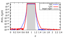
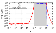
(a) $[a,b]=[0.8,1.2]$. (b) $[a,b]=[10^{-3},10^{-1}]$.

Figure 1: The values of $|f(\sigma)|$ and $|f_{g}(\sigma)|$.

As shown in Figure 1(a), in the case that the target region is around 1, there is no large difference between the filter functions $f(\sigma)$ and $f_{g}(\sigma)$. On the other hand, as shown in Figure 1(b), in the case that the target region is cross to 0, there is large difference. For the region of $\sigma>b$, both $|f(\sigma)|$ and $|f_{g}(\sigma)|$ decrease with increasing $\sigma$, specifically $|f(\sigma)|$ shows rapid decreasing. For the region of $0<\sigma<a$, $|f(\sigma)|$ shows large value $|f(\sigma)|\approx 0.5$. Instead, $|f_{g}(\sigma)|$ drastically decrease. This result indicates that, a cluster of singular value in the region $[0,10^{-4}]$ causes a negative effect on the accuracy of the SS-SVD based on $f(\sigma)$, but not the accuracy of the SS-SVD with nonlinear transform based on $f_{g}(\sigma)$.

4.2 Experiment II: model problem

In this subsection, we compare the accuracy of four methods:

• Naive: The block SS–CAA method [16] via the symmetric eigenvalue problem (2);

• Naive with NT: Naive with the nonlinear trasnform;

• SS–SVD: The proposed method (Algorithm 1);

• SS–SVD with NT: The proposed method with the nonlinear trainsform (Algorithm 2),

using two small model problems of size $m=1000,n=200$. For the model problem 1, we set

$$\Sigma={\rm diag}(0.005,0.015,\ldots,1.995)\in\mathbb{R}^{200\times 200}$$ (18)

such that singular values are uniformly distributed, and for the model problem 2, we set

$$\Sigma={\rm diag}(10^{-10.0},10^{-9.95},\ldots,10^{-0.05})\in\mathbb{R}^{200\times 200}$$ (19)

such that singular values are uniformly distributed on the logarithmic scale. Then, the matrix $A$ is constructed as $A=U\Sigma V^{\rm T}$ with orthogonal matrices $U$ and $V$ constructed from random matrices.

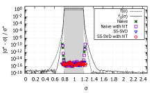
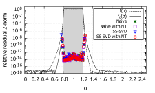
(a) The model problem 1 (18).
 
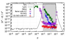
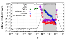
(b) The model problem 2 (19).

Figure 2: Relative error $|\sigma_{i}^{\ast}-\sigma_{i}|/\sigma_{i}^{\ast}$ of singular values and residual 2-norm $\|{\bm{r}}_{i}\|_{2}$.

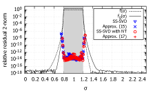
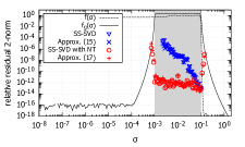
(a) The model problem 1 (18). (b) The model problem 2 (19).

Figure 3: Residual norm and its approximation.

For the model problem 1, we compute 40 singular triplets such that $\sigma_{i}\in[0.8,1.2]$ and for the model problem 2, we compute 40 singular triplets such that $\sigma_{i}\in[10^{-3},10^{-1}]$. We set the parameters as $(L,M,N,\ell,\delta)=(20,4,32,1$, $10^{-20})$.

In Figure 2, we show relative error of singular value $|\sigma_{i}^{\ast}-\widehat{\sigma}_{i}|/\sigma_{i}^{\ast}$, where $\sigma_{i}^{\ast}$ is the exact singular value, and residual 2-norm $\|{\bm{r}}_{i}\|_{2}=\|A^{\rm T}\widehat{\bm{u}}_{i}-\widehat{\sigma}_{i}\widehat{\bm{v}}_{i}\|_{2}$. In the case of the model problem 1 (18) whose singular values are uniformly distributed, as shown in Figure 2(a), all methods show almost the same accuracy both for the relative error and residual 2-norm. On the other hand, in the case of the model problem 2 (19) whose singular values are uniformly distributed on the logarithmic scale, as shown in Figure 2(b), the nonlinear transformation shows drastically improves the accuracy. Specifically, the SS-SVD with the nonlinear transformation shows the best results both for relative error and residual 2-norm.

In Figure 3, we show the residual 2-norm and its estimations (15) and (17) for the proposed methods. We observe that the both approximations well estimated the exact residual 2-norms for both problems.

4.3 Experiment III: real-world problem

We evaluate the computation time of the proposed method compared with that of MATLAB functions svd for computing all the singular triplets and svds for computing partial singular triplets. We used a $60000\times 784$ sparse matrix obtained from a 10-class classification of handwritten digits (MNIST) [21]. The average nonzero elements per row is 149.9. We normalized the matrix as the largest singular value is 1. For svds, we computed the largest $10,20,\dots,160$ singular triplets. For the proposed method, the target interval, the number $t$ of the target singular triplets and parameters $L,M$ are shown in Table 1. Here, we fix $M=4$ and set $L$ as $LM\approx 3t$. We also set $(N,\ell,\delta)=(32,1,10^{-20})$.

Table 1: The target region $[a,b]$, the number $t$ of the target singular triplets and parameter setting for the proposed method.

Exterior					Interior
$[a,b]$	$t$	$L$	$M$		$[a,b]$	$t$	$L$	$M$
$[0.120,1.01]$	21	15	4		$[0.060,0.08]$	17	15	4
$[0.080,1.01]$	40	30	4		$[0.045,0.08]$	39	30	4
$[0.045,1.01]$	79	60	4		$[0.030,0.08]$	85	60	4
$[0.025,1.01]$	153	120	4		$[0.020,0.08]$	158	120	4

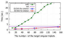
Figure 4: The computation time v.s. the number of the target singular triplets.

Table 2: Breakdown of the computation time and accuracy of the proposed method.

Exterior
region		Computation time [sec.]						accuracy
$[a,b]$		Steps 1–2	3	4	5	Total		error	residual
$[0.120,1.01]$		0.809	0.002	0.144	0.006	0.962		1.67E-15	1.57E-13
$[0.080,1.01]$		0.842	0.005	0.299	0.017	1.146		1.70E-15	1.90E-14
$[0.045,1.01]$		0.886	0.015	0.792	0.049	1.693		2.94E-15	1.03E-14
$[0.025,1.01]$		0.997	0.054	1.847	0.178	2.898		2.48E-15	3.90E-15
Interior
region		Computation time [sec.]						accuracy
$[a,b]$		Steps 1–2	3	4	5	Total		error	residual
$[0.060,0.08]$		0.830	0.002	0.150	0.006	0.983		1.09E-15	8.26E-14
$[0.045,0.08]$		0.858	0.005	0.286	0.017	1.148		2.62E-15	8.99E-14
$[0.030,0.08]$		0.886	0.015	0.795	0.047	1.695		2.18E-15	5.02E-13
$[0.020,0.08]$		1.024	0.056	1.762	0.184	2.842		2.48E-15	3.99E-16

The computation time of all methods are shown in Figure 4. The breakdown of the computation time and accuracy of the proposed method are also shown in Table 2. As shown in Figure 4, the computation time of svds increases with increasing the number $t$ of the target singular values. Then, in this experiment, svd is faster than svds when $t>30$. Instead, the proposed method is much faster than svds and svd for both exterior and interior cases, although the computation time, specifically Step 4, of the proposed method increases with increasing $t$ and $L$.

5 Conclusions

Based on the concept of the complex moment-based eigensolvers, in this paper, we proposed a novel complex moment-based method to compute interior singular triplets (1). We also analysed error bounds of the proposed method and proposed an improvement technique using a nonlinear transformation to improve accuracy of the proposed method. The proposed method has high parallel efficiency as the complex moment-based parallel eigensolvers. From the numerical experiments, the proposed complex moment-based method with the nonlinear transformation can compute accurate singular triplets for both exterior and interior problems. The computation time of the proposed method is much faster than svds and svd.

In the future, we will evaluate the parallel performance of the proposed method for more large real-world problems.

References

- [1] J. Asakura, T. Sakurai, H. Tadano, T. Ikegami, K. Kimura, A numerical method for nonlinear eigenvalue problems using contour integrals, JSIAM Letters 1 (2009) 52–55.
- [2] J. Asakura, T. Sakurai, H. Tadano, T. Ikegami, K. Kimura, A numerical method for polynomial eigenvalue problems using contour integral, Japan Journal of Industrial and Applied Mathematics 27 (1) (2010) 73–90.
- [3] W.-J. Beyn, An integral method for solving nonlinear eigenvalue problems, Linear Algebra and its Applications 436 (10) (2012) 3839–3863.
- [4] F. Chatelin, Eigenvalues of Matrices, Wiley, Chichester, 1993.
- [5] FEAST Eigenvalue Solver, http://www.ecs.umass.edu/~polizzi/feast/.
- [6] G. H. Golub, C. F. Van Loan, Matrix Computations, 3rd ed., The Johns Hopkins University Press, 1996.
- [7] S. Güttel, E. Polizzi, P. T. P. Tang, G. Viaud, Zolotarev quadrature rules and load balancing for the FEAST eigensolver, SIAM Journal on Scientific Computing 37 (4) (2015) A2100–A2122.
- [8] M. E. Hochstenbach, A Jacobi–Davidson type SVD method, SIAM J. Sci. Comput. 23 (2001) 606–628.
- [9] T. Ikegami, T. Sakurai, Contour integral eigensolver for non-Hermitian systems: a Rayleigh-Ritz-type approach, Taiwanese Journal of Mathematics (2010) 825–837.
- [10] T. Ikegami, T. Sakurai, U. Nagashima, A filter diagonalization for generalized eigenvalue problems based on the Sakurai–Sugiura projection method, Journal of Computational and Applied Mathematics 233 (8) (2010) 1927–1936.
- [11] A. Imakura, L. Du, T. Sakurai, A block Arnoldi-type contour integral spectral projection method for solving generalized eigenvalue problems, Applied Mathematics Letters 32 (2014) 22–27.
- [12] A. Imakura, L. Du, T. Sakurai, Error bounds of Rayleigh–Ritz type contour integral-based eigensolver for solving generalized eigenvalue problems, Numer. Alg. 71 (2016) 103–120.
- [13] A. Imakura, L. Du, T. Sakurai, Relationships among contour integral-based methods for solving generalized eigenvalue problems, Japan Journal of Industrial and Applied Mathematics 33 (3) (2016) 721–750.
- [14] A. Imakura, Y. Futamura, T. Sakurai, Structure-preserving technique in the block SS–Hankel method for solving Hermitian generalized eigenvalue problems, in: International Conference on Parallel Processing and Applied Mathematics, Springer, 2017.
- [15] A. Imakura, M. Matsuda, X. Ye, T. Sakurai, Complex moment-based supervised eigenmap for dimensionality reduction, in: Proceedings of the AAAI Conference on Artificial Intelligence, vol. 33, 2019.
- [16] A. Imakura, T. Sakurai, Block Krylov-type complex moment-based eigensolvers for solving generalized eigenvalue problems, Numerical Algorithms 75 (2) (2017) 413–433.
- [17] A. Imakura, T. Sakurai, Block SS-CAA: A complex moment-based parallel nonlinear eigensolver using the block communication-avoiding Arnoldi procedure, Parallel Computing (2018) 34–48.
- [18] S. Iwase, Y. Futamura, A. Imakura, T. Sakurai, T. Ono, Efficient and scalable calculation of complex band structure using Sakurai-Sugiura method, in: Proceedings of the International Conference for High Performance Computing, Networking, Storage and Analysis, ACM, 2017.
- [19] J. Kestyn, V. Kalantzis, E. Polizzi, Y. Saad, PFEAST: a high performance sparse eigenvalue solver using distributed-memory linear solvers, in: High Performance Computing, Networking, Storage and Analysis, SC16: International Conference for, IEEE, 2016.
- [20] J. Kestyn, E. Polizzi, P. T. Peter Tang, FEAST eigensolver for non-hermitian problems, SIAM Journal on Scientific Computing 38 (5) (2016) S772–S799.
- [21] Y. LeCun, The MNIST database of handwritten digits, http://yann. lecun. com/exdb/mnist/.
- [22] N.Halko, P.G.Martinsson, J. A.Tropp, Finding structure with randomness: probabilistic algorithms for constructing approximate matrix decompositions, SIAM Rev. 53 (2011) 217–288.
- [23] E. Polizzi, A density matrix-based algorithm for solving eigenvalue problems, Phys. Rev. B 79 (2009) 115112.
- [24] Y. Saad, Numerical Methods for Large Eigenvalue Problems, 2nd ed., Manchester University Press, 2011.
- [25] T. Sakurai, Y. Futamura, A. Imakura, T. Imamura, Scalable eigen-analysis engine for large-scale eigenvalue problems, in: Sato M. (eds) Advanced Software Technologies for Post-Peta Scale Computing, Springer, Singapore, 2019.
- [26] T. Sakurai, H. Sugiura, A projection method for generalized eigenvalue problems using numerical integration, Journal of computational and applied mathematics 159 (1) (2003) 119–128.
- [27] T. Sakurai, H. Tadano, CIRR: a Rayleigh-Ritz type method with counter integral for generalized eigenvalue problems, Hokkaido Math. J. 36 (2007) 745–757.
- [28] G. Schofield, J. R. Chelikowsky, Y. Saad, A spectrum slicing method for the kohn-sham problem, Comput. Phys. Commun. 183 (2012) 497–505.
- [29] P. T. P. Tang, E. Polizzi, FEAST as a subspace iteration eigensolver accelerated by approximate spectral projection, SIAM Journal on Matrix Analysis and Applications 35 (2) (2014) 354–390.
- [30] M. Van Barel, P. Kravanja, Nonlinear eigenvalue problems and contour integrals, Journal of Computational and Applied Mathematics 292 (2016) 526–540.
- [31] T. Yano, Y. Futamura, A. Imakura, T. Sakurai, Efficient implementation of a dimensionality reduction method using a complex moment-based subspace, in: The International Conference on High Performance Computing in Asia-Pacific Region, HPC Asia 2021, 2021.
- [32] S. Yokota, T. Sakurai, A projection method for nonlinear eigenvalue problems using contour integrals, JSIAM Letters 5 (2013) 41–44.
- [33] z-Pares: Parallel Eigenvalue Solver, http://zpares.cs.tsukuba.ac.jp/.