Gaussian and Student’s t mixture vector autoregressive model with application to the asymmetric effects of monetary policy shocks in the Euro area

Savi Virolainen
University of Helsinki

A new mixture vector autoregressive model based on Gaussian and Student’s $t$ distributions is introduced. As its mixture components, our model incorporates conditionally homoskedastic linear Gaussian vector autoregressions and conditionally heteroskedastic linear Student’s $t$ vector autoregressions. For a $p$th order model, the mixing weights depend on the full distribution of the preceding $p$ observations, which leads to attractive theoretical properties such as ergodicity and full knowledge of the stationary distribution of $p+1$ consecutive observations. A structural version of the model with statistically identified shocks and a time-varying impact matrix is also proposed. The empirical application studies asymmetries in the effects of the Euro area monetary policy shock. Our model identifies two regimes: a high-growth regime that is characterized by positive output gap and mainly prevailing before the Financial crisis, and a low-growth regime that characterized by negative but volatile output gap and mainly prevailing after the Financial crisis. The average inflationary effects of the monetary policy shock are stronger in the high-growth regime than in the low-growth regime. On average, the effects of an expansionary shock are less enduring than of a contractionary shock. The CRAN distributed R package gmvarkit accompanies the paper.

Keywords: mixture vector autoregression, regime-switching, Student’s t mixture, Gaussian mixture, mixture model, Euro area monetary policy shock

1 Introduction

Mixture autoregressive models are useful for modelling series in which the data generating dynamics vary in time. Such variation may arise due to wars, crises, business cycle fluctuations, or policy shifts, for example. Mixture autoregressive models can be described as collections of (typically linear) autoregressive models, which are called mixture components, components processes, or regimes. At each time point, the process generates an observation from one of its mixture components that is randomly selected according to the probabilities given by the mixing weights.

Several new mixture autoregressive models have been introduced recently. Kalliovirta et al. (2015) introduced the Gaussian mixture autoregressive (GMAR) model, which incorporates linear Gaussian autoregressions as its mixture components and mixing weights that, for a $p$th order model, depend on the full distribution of the previous $p$ observations. The specific definition of the mixing weights leads to attractive theoretical and practical properties, such as ergodicity and full knowledge of the stationary distribution of $p+1$ consecutive observations. Kalliovirta et al. (2016) introduced a multivariate version of this model, the Gaussian mixture vector autoregressive (GMVAR) model, which employs linear Gaussian vector autoregressions (VAR) as its mixture components and has analogous properties to the GMAR model. Burgard et al. (2019), in turn, proposed a model with linear Gaussian VARs as mixture components, and mixing weights that depend on switching variables through a logistic function. Meitz et al. (forthcoming) introduced the Student’s $t$ mixture autoregressive (StMAR) model with analogous properties to the GMAR model, but incorporating conditionally heteroskedastic mixture components based on Student’s $t$-distribution. Virolainen (forthcoming) introduced the Gaussian and Student’s $t$ mixture autoregressive (G-StMAR) model, where some of the mixture components are based on a Gaussian distribution and some on a $t$-distribution.

This paper introduces a multivariate version of the G-StMAR model, and as a special case also a multivariate version of the StMAR model. The Gaussian and Student’s $t$ mixture vector autoregressive (G-StMVAR) model accommodates conditionally homoskedastic linear Gaussian VARs and conditionally heteroskedastic linear Student’s $t$ VARs as its mixture components. Both types of mixture components have the same form for the conditional mean, a linear function of the preceding $p$ observations, but the conditional covariance matrices are different. The linear Gaussian VARs have constant conditional covariance matrices. The conditional covariance matrices of the linear Student’s $t$ VARs, in turn, consist of a constant covariance matrix multiplied by a time-varying scalar that depends on the quadratic form of the previous $p$ observations. In this sense, the conditional covariance is of ARCH (autoregressive conditional heteroskedasticity) type. But since it is just a time-varying scalar multiplying the constant covariance matrix, it is not as general as the conventional multivariate ARCH process that allows the entries of the conditional covariance matrix to vary relative to each other (e.g., Lütkepohl, 2005, Section16.3). The specific formulation of the conditional covariance matrix is, nonetheless, convenient for establishing stationary properties similar to the linear Gaussian VARs. Our specification of the conditional covariance matrix is also parsimonious, as it only depends on the degrees of freedom and the autoregressive parameters (in addition to the parameters in the constant covariance matrix). This is particularly advantegeous in the context of mixture VARs, as the large number of parameters may often be a problem even without an ARCH component.

For a $p$th order G-StMVAR model, the mixing weights are defined as weighted ratios of the components process stationary densities corresponding the previous $p$ observations. This formulation is appealing, as it states that the greater the relative weighted likelihood of a regime is, the more likely the process is to generate an observation from it. This is a convenient feature for forecasting, and it also facilitates associating statistical characteristics and economic interpretations to the regimes. It turns out that the specific formulation of the mixing weights also leads to attractive theoretical properties, such as ergodicity and full knowledge of the stationary distribution of $p+1$ consecutive observations. In contrast to the GMVAR model, our model is able to capture excess kurtosis and conditional heteroskedasticity within the regimes. If all of the regimes are assumed to be linear Student’s $t$ VARs, a multivariate version of the StMAR model is obtained as a special case. We refer to this model as the StMVAR model.

In addition to the reduced form model, we propose a structural version of the G-StMVAR model that generalizes the SGMVAR model of Virolainen (2022) to accommodate conditionally heteroskedastic Student’s $t$ regimes. The SG-StMVAR model incorporates a time-varying impact matrix that varies according to the conditional variance of the reduced form error. As a consequence of a single (time-varying) impact matrix, identification of the shocks requires that the error term covariance matrices are simultaneously diagonalized in all regimes. Together with a constant normalization of the structural error’s conditional covariance matrix, this condition generally leads to uniquely identified shocks up to ordering and sign. Hence, as long as one is willing to assume a single (time-varying) impact matrix, its columns characterize the estimated impact effects of the shocks, but it is not revealed which column is related to which shock. Because the impact matrix is also subject to estimation error, further constraints may be needed for labelling the shocks. The identification conditions are the same as in Virolainen (2022), however, and we repeat some of them for convenience.

The empirical application studies asymmetries in the expected effects of the monetary policy shock in the Euro area and considers a monthly data covering the period from January 1999 to December 2021. Our StMVAR model identifies two regimes: a low-growth regime and a high-growth regime. The low-growth regime is characterized by a negative (but volatile) output gap, and it mainly prevails after the collapse of Lehman Brothers in the Financial crisis but obtains large mixing weights also during and before the early 2000’s recession. The high-growth regime is characterized by a positive output gap and it mainly dominates before the Financial crisis.

We find strong asymmetries with respect to the initial state of the economy and sign of the shock, but asymmetries with respect to the size of the shock are weak. The real effects are less enduring for an expansionary shock than for a contractionary shock. Particularly in the high-growth regime, a contractionary shock persistently drives the economy towards the low-growth regime, which translates to a very persistent decrease in the output gap. The inflationary effects of the monetary policy shock are stronger in the high-growth regime than in the low-growth regime, and in the latter the price level does not move much on average.

The rest of this paper is organized as follows. Section 2 introduces the linear Student’s $t$ VAR and establishes its stationary properties. Section 3 introduces the G-StMVAR model and discusses its properties. Section 4 introduces the structural G-StMVAR model and briefly discusses identification of the shocks. Section 5 discusses estimation of the model parameters by the method of maximum likelihood (ML) and establishes the asymptotic properties of the ML estimator. Section 6 discusses a strategy for building a G-StMVAR model, and Section 7 presents the empirical application to the asymmetric effects of the Euro area monetary policy shock. Appendix A provides the density functions and some properties of the Gaussian and Student’s $t$ distributions, Appendix B gives proofs for the stated theorems, and Appendix C provides details on the empirical application. Finally, this paper is accompanied with the CRAN distributed R package gmvarkit (Virolainen, 2018a) that provides tools for estimation and other numerical analysis of the models.

Throughout this paper, we use the following notation. We write $x=(x_{1},...,x_{n})$ for the column vector $x$ where the components $x_{i}$ may be either scalars or (column) vectors. The notation $x\sim n_{d}(\mu,\Sigma)$ signifies that the random vector $x$ has a $d$-dimensional Gaussian distribution with mean $\mu$ and (positive definite) covariance matrix $\Sigma$, and $n_{d}(\cdot;\mu,\Sigma)$ denotes the corresponding density function. Similarly, $x\sim t_{d}(\mu,\Sigma,\nu)$ signifies that $x$ has a $d$-dimensional $t$-distribution with mean $\mu$, (positive definite) covariance matrix $\Sigma$, and degrees of freedom $\nu$ (assumed to satisfy $\nu>2$), and $t_{d}(\cdot;\mu,\Sigma,\nu)$ denotes the corresponding density function. The vectorization operator $vec$ stacks columns of a matrix on top of each other and $vech$ stacks them from the main diagonal downwards (including the main diagonal). The $(d\times d)$ identity matrix is denoted by $I_{d}$, $\otimes$ denotes the Kronecker product, and $\boldsymbol{1}_{d}$ denotes a $d$-dimensional vectors of ones.

2 Linear Gaussian and Student’s t vector autoregressions

The G-StMVAR model accommodates two types of mixture components: conditionally homoskedastic linear Gaussian vector autoregressions and conditionally heteroskedastic linear Student’s $t$ vector autoregressions. This section defines these linear vector autoregressions and establishes their stationary properties. Consider the $d$-dimensional linear VAR model defined as

$$z_{t}=\phi_{0}+\sum_{i=1}^{p}A_{i}z_{t-1}+\Omega_{t}^{1/2}\varepsilon_{t},$$ (2.1)

where the error process $\varepsilon_{t}$ identically and independently distributed (IID), $\Omega_{t}^{1/2}$ is a symmetric square root matrix of the positive definite $(d\times d)$ covariance matrix $\Omega_{t}$ for all $t$, and $\phi_{0}\in\mathbb{R}^{d}$. The $(d\times d)$ autoregression matrices are assumed to satisfy $\boldsymbol{A}_{p}\equiv[A_{1}:...:A_{p}]\in\mathbb{S}^{d\times dp}$, where

$$\mathbb{S}^{d\times dp}=\{[A_{1}:...:A_{p}]\in\mathbb{R}^{d\times dp}:\det(I_{d}-\sum_{i=1}^{p}A_{i}z^{i})\neq 0\ \text{for}\ |z|\leq 1\}$$ (2.2)

defines the usual stability condition of a linear VAR. The linear Gaussian VAR is obtained from Equation (2.1) by assuming that $\varepsilon_{t}$ follows the $d$-dimensional standard normal distribution and that the conditional covariance matrix is a constant, $\Omega_{t}=\Omega$. We will first establish the stationary properties of the linear Gaussian VAR, and by making use of the introduced notation, we then introduce the linear Student’s $t$ VAR.

Under the stability condition, the linear Gaussian VAR is stationary, and the following properties are obtained. Denoting $\boldsymbol{z}_{t}=(z_{t},...,z_{t-p+1})$ and $\boldsymbol{z}_{t}^{+}=(z_{t},\boldsymbol{z}_{t-1})$, it is well known that the stationary solution to (2.1) satisfies

$$\begin{aligned} \boldsymbol{z}_{t}&\sim n_{dp}(\boldsymbol{1}_{p}\otimes\mu,\Sigma_{p})\\ \boldsymbol{z}^{+}_{t}&\sim n_{d(p+1)}(\boldsymbol{1}_{p+1}\otimes\mu,\Sigma_{p+1})\\ z_{t}|\boldsymbol{z}_{t-1}&\sim n_{d}(\mu+\Sigma_{1p}\Sigma_{p}^{-1}(\boldsymbol{z}_{t-1}-\boldsymbol{1}_{p}\otimes\mu),\Sigma_{1}-\Sigma_{1p}\Sigma_{p}^{-1}\Sigma_{1p}^{\prime})=n_{d}(\phi_{0}+\boldsymbol{A}_{p}\boldsymbol{z}_{t-1},\Omega),\end{aligned}$$ (2.3)

where the last line defines the conditional distribution of $z_{t}$ given $\boldsymbol{z}_{t-1}$. Denoting by $\Sigma(h)$, $h=0,\pm 1,\pm 2,...$, the lag $h$ autocovariance matrix of $z_{t}$, the quantities $\mu,\Sigma_{p},\Sigma_{1},\Sigma_{1p},\Sigma_{p+1}$ are given as (see, e.g., Lütkepohl, 2005, pp. 23, 28-29)

$$\begin{aligned} \mu=&(I_{d}-\sum_{i=1}^{p}A_{i})^{-1}\phi_{0}&(d\times 1)\\ \text{vec}(\Sigma_{p})=&(I_{(dp)^{2}}-\boldsymbol{A}\otimes\boldsymbol{A})^{-1}\text{vec}(\boldsymbol{\Omega})&((dp)^{2}\times 1)\\ \Sigma_{1}=&\Sigma(0)&(d\times d)\\ \Sigma(p)=&A_{1}\Sigma(p-1)+\cdots+A_{p}\Sigma(0)&(d\times d)\\ \Sigma_{1p}=&[\Sigma(1):...:\Sigma(p-1):\Sigma(p)]=\boldsymbol{A}_{p}\Sigma_{p}&(d\times dp)\\ \Sigma_{p+1}=&\begin{bmatrix}\Sigma_{1}&\Sigma_{1p}\\ \Sigma_{1p}^{\prime}&\Sigma_{p}\end{bmatrix}&(d(p+1)\times d(p+1))\end{aligned}$$ (2.4)

where

$$\Sigma_{p}=\underset{(dp\times dp)}{\begin{bmatrix}\Sigma(0)&\Sigma(1)&\cdots&\Sigma(p-1)\\ \Sigma(-1)&\Sigma(0)&\cdots&\Sigma(p-2)\\ \vdots&\vdots&\ddots&\vdots\\ \Sigma(-p+1)&\Sigma(-p+2)&\cdots&\Sigma(0)\\ \end{bmatrix}},\quad\boldsymbol{\Omega}=\underset{(dp\times dp)}{\begin{bmatrix}\Omega&0&\cdots&0\\ 0&0&\cdots&0\\ \vdots&\vdots&\ddots&\vdots\\ 0&0&\ldots&0\end{bmatrix}},$$ (2.5)

and

$$\boldsymbol{A}=\underset{(dp\times dp)}{\begin{bmatrix}A_{1}&A_{2}&\cdots&A_{p-1}&A_{p}\\ I_{d}&0&\cdots&0&0\\ 0&I_{d}&&0&0\\ \vdots&&\ddots&\vdots&\vdots\\ 0&0&\ldots&I_{d}&0\end{bmatrix}}.$$ (2.6)

In order to construct a linear Student’s $t$ VAR with stationary properties analogous to (2.3), we consider the appropriate marginal distribution of $p+1$ consecutive observations. Then, a connection to the VAR (2.1) is made through the conditional distribution, and finally this process and its stationary properties are formally established. Suppose that for a random vector in $\mathbb{R}^{d(p+1)}$ it holds that $(z,\boldsymbol{z})\sim t_{d(p+1)}(\boldsymbol{1}_{p+1}\otimes\mu,\Sigma_{p+1},\nu)$, where $\nu>2$. By the properties of a multivariate Student’s $t$-distribution (given in Appendix A), the conditional distribution of $z$ given $\boldsymbol{z}$ is $z|\boldsymbol{z}\sim t_{d}(\mu(\boldsymbol{z}),\Omega(\boldsymbol{z}),\nu+dp)$, where

$$\mu(\boldsymbol{z})= \phi_{0}+\boldsymbol{A}_{p}\boldsymbol{z}$$ (2.7)

$$\Omega(\boldsymbol{z})= \frac{\nu-2+(\boldsymbol{z}-\boldsymbol{1}_{p}\otimes\mu)^{\prime}\Sigma_{p}^{-1}(\boldsymbol{z}-\boldsymbol{1}_{p}\otimes\mu)}{\nu-2+dp}\Omega.$$ (2.8)

It is easy to see that a VAR of the form (2.1) that has the above-described conditional Student’s $t$-distribution is obtained by assuming that $\varepsilon_{t}\sim t_{d}(0,I_{d},\nu+dp)$ and that the conditional covariance matrix $\Omega_{t}$ is of the form (2.8). The following theorem then formally establishes this Student’s $t$ VAR and its stationary properties (which is analogous to Theorem 1 in Meitz et al., forthcoming, considering a univariate version of the Student’s $t$ autoregression).

Theorem 1.

Suppose $\phi_{0}\in\mathbb{R}^{d}$, $[A_{1}:...:A_{p}]\in\mathbb{S}^{d\times dp}$,$\Omega\in\mathbb{R}^{d\times d}$ is positive definite, and that $\nu>2$. Then, there exists a process $\boldsymbol{z}_{t}=(z_{t},...,z_{t-p+1})$ $(t=0,1,2,...)$ with the following properties.

1. The process $\boldsymbol{z}_{t}$ is a Markov chain on $\mathbb{R}^{dp}$ with a stationary distribution characterized by the density function $t_{dp}(\boldsymbol{1}_{p}\otimes\mu,\Sigma_{p},\nu)$. When $\boldsymbol{z}_{0}\sim t_{dp}(\boldsymbol{1}_{p}\otimes\mu,\Sigma_{p},\nu)$, we have, for $t=1,2,...,$ that $\boldsymbol{z}_{t}^{+}\sim t_{d(p+1)}(\boldsymbol{1}_{p+1}\otimes\mu,\Sigma_{p+1},\nu)$ and the conditional distribution of $z_{t}$ given $\boldsymbol{z}_{t-1}$ is

   $$z_{t}|\boldsymbol{z}_{t-1}\sim t_{d}(\mu(\boldsymbol{z}_{t-1}),\Omega(\boldsymbol{z}_{t-1}),\nu+dp).$$ (2.9)

2. Furthermore, for $t=1,2,...$, the process $z_{t}$ has the representation

   $$z_{t}=\phi_{0}+\sum_{i=1}^{p}A_{i}z_{t-i}+\Omega_{t}^{1/2}\varepsilon_{t},$$ (2.10)

   where $\Omega_{t}=\Omega(\boldsymbol{z}_{t-1})$ is the conditional covariance matrix (see (2.8)), $\varepsilon_{t}\sim\text{IID}\ t_{d}(0,I_{d},\nu+dp)$, and $\varepsilon_{t}$ are independent of $\{z_{t-j},j>0\}$ for all $t$.

Analogously to the univariate linear Student’s autoregression discussed in Meitz et al. (forthcoming), the results 2.9 and 2.10 in Theorem 1 are comparable to properties (2.3) and (2.1) of the Gaussian counterpart. Part 2.9 shows that both the stationary and conditional distributions of $z_{t}$ are $t$–distributions, whereas part (ii) clarifies the connection to the standard VAR model.

Our Student’s $t$ VAR has a conditional mean identical to the Gaussian VAR, but unlike the Gaussian VAR, it is conditionally heteroskedastic. Specifically, the conditional variance (2.8) consists of a constant covariance matrix that is multiplied by a time-varying scalar that depends on the quadratic form of the preceding $p$ observations through the autoregressive parameters. In this sense, the model has a ‘VAR($p$)–ARCH($p$)’ representation, but the ARCH type conditional variance is not as general as in the conventional multivariate ARCH process (e.g., Lütkepohl, 2005, Section 16.3) that allows the entries of the conditional covariance matrix to vary relative to each other. Our model is, however, more parsimonious than the conventional VAR-ARCH model, as the conditional covariance depends only on the degrees of freedom and autoregressive parameters (in addition to the parameters in the constant covariance matrix). Student’s $t$ VARs similar to ours have previously appeared at least in Heracleous (2003) and Poudyal (2012).

3 The Gaussian and Student’s t mixture vector autoregressive model

The G-StMVAR model can be described as a collection of linear autoregressive models that are the linear Gaussian VARs or the linear Student’s $t$ VARs defined in Section 2. At each time point, the process generates an observation from one of its mixture components that is randomly selected according to the probabilities given by the mixing weights. This definition is formalized next.

Let $y_{t}$ $(t=1,2,...)$ be the real valued $d$-dimensional time series of interest, and let $\mathcal{F}_{t-1}$ denote $\sigma$-algebra generated by the random vectors $\{y_{s},s<t\}$. In a G-StMVAR model with autoregressive order $p$ and $M$ mixture components (or regimes), the observations $y_{t}$ are assumed to be generated by

$$y_{t}= \sum_{m=1}^{M}s_{m,t}(\mu_{m,t}+\Omega_{m,t}^{1/2}\varepsilon_{m,t}),$$ (3.1)

$$\mu_{m,t}= \phi_{m,0}+\sum_{i=1}^{p}A_{m,i}y_{t-i},$$ (3.2)

where the following conditions hold (which are similar to Condition 1 in Kalliovirta et al., 2016).

Condition 1.

1. For $m=1,...,M_{1}\leq M$, the random vectors $\varepsilon_{m,t}$ are IID $n_{d}(0,I_{d})$ distributed, and for $m=M_{1}+1,...,M$, they are IID $t_{d}(0,I_{d},\nu_{m}+dp)$ distributed. For all $m$, $\varepsilon_{m,t}$ are independent of $\mathcal{F}_{t-1}$.

2. For each $m=1,...,M$‚ $\phi_{m,0}\in\mathbb{R}^{d}$, $\boldsymbol{A}_{m,p}\equiv[A_{m,1}:...:A_{m,p}]\in\mathbb{S}^{d\times dp}$ (the set $\mathbb{S}^{d\times dp}$ is defined in (2.2)), and $\Omega_{m}$ is positive definite. For $m=1,...,M_{1}$, the conditional covariance matrices are constants, $\Omega_{m,t}=\Omega_{m}$. For $m=M_{1}+1,...,M$, the conditional covariance matrices $\Omega_{m,t}$ are as in (2.8), except that $\boldsymbol{z}$ is replaced with $\boldsymbol{y}_{t-1}=(y_{t-1},...,y_{t-p})$ and the regime specific parameters $\phi_{m,0}$, $\boldsymbol{A}_{m,p}$,$\Omega_{m}$,$\nu_{m}$ are used to define the quantities therein. For $m=M_{1}+1,...,M$, also $\nu_{m}>2$.

3. The unobservable regime variables $s_{1,t},...,s_{M,t}$ are such that at each $t$, exactly one of them takes the value one and the others take the value zero according to the conditional probabilities expressed in terms of the ($\mathcal{F}_{t-1}$-measurable) mixing weights $\alpha_{m,t}\equiv\mathrm{P}(s_{m,t}=1|\mathcal{F}_{t-1})$ that satisfy $\sum_{m=1}^{M}\alpha_{m,t}=1$.

4. Conditionally on $\mathcal{F}_{t-1}$, $(s_{1,t},...,s_{M,t})$ and $\varepsilon_{m,t}$ are assumed independent.

The conditions $\nu_{m}>2$ in (b) are made to ensure the existence of second moments. This definition implies that the G-StMVAR model generates each observation from one of its mixture components, a linear Gaussian or Student’s $t$ vector autoregression discussed in Section 2, and that the mixture component is selected randomly according to the probabilities given by the mixing weights $\alpha_{m,t}$.

The first $M_{1}$ mixture components are assumed to be linear Gaussian VARs, and the last $M_{2}\equiv M-M_{1}$ mixture components are assumed to be linear Student’s $t$ VARs. If all the component processes are Gaussian VARs ($M_{1}=M$), the G-StMVAR model reduces to the GMVAR model of Kalliovirta et al. (2016). If all the component processes are Student’s $t$ VARs ($M_{1}=0$), we refer to the model as the StMVAR model.

Equations (3.1) and (3.2) and Condition 1 lead to a model in which the conditional density function of $y_{t}$ conditional on its past, $\mathcal{F}_{t-1}$, is given as

$$f(y_{t}|\mathcal{F}_{t-1})=\sum_{m=1}^{M_{1}}\alpha_{m,t}n_{d}(y_{t};\mu_{m,t},\Omega_{m})+\sum_{m=M_{1}+1}^{M}\alpha_{m,t}t_{d}(y_{t};\mu_{m,t},\Omega_{m,t},\nu_{m}+dp).$$ (3.3)

The conditional densities $n_{d}(y_{t};\mu_{m,t},\Omega_{m,t})$ are obtained from (2.3), whereas $t_{d}(y_{t};\mu_{m,t},\Omega_{m,t},\nu_{m}+dp)$ are obtained from Theorem 1. The explicit expressions of the density functions are given in Appendix A. To fully define the G-StMVAR model it is then left to specify the mixing weights.

Analogously to Kalliovirta et al. (2015), Kalliovirta et al. (2016), Meitz et al. (forthcoming), and Virolainen (forthcoming), we define the mixing weights as weighted ratios of the component process stationary densities corresponding to the previous $p$ observations. In order to formally specify the mixing weights, we first define the following function for notational convenience. Let

$$d_{m,dp}(\boldsymbol{y};\mathbf{1}_{p}\otimes\mu_{m},\Sigma_{m,p},\nu_{m})=\left\{\begin{matrix}[l]n_{dp}(\boldsymbol{y};\mathbf{1}_{p}\otimes\mu_{m},\Sigma_{m,p}),&\text{when}\ m\leq M_{1},\\ t_{dp}(\boldsymbol{y};\mathbf{1}_{p}\otimes\mu_{m},\Sigma_{m,p},\nu_{m}),&\text{when}\ m>M_{1},\end{matrix}\right.$$ (3.4)

where the $dp$-dimensional densities $n_{dp}(\boldsymbol{y};\mathbf{1}_{p}\otimes\mu_{m},\Sigma_{m,p})$ and $t_{dp}(\boldsymbol{y};\mathbf{1}_{p}\otimes\mu_{m},\Sigma_{m,p},\nu_{m})$ correspond to the stationary distribution of the $m$th component process (given in Equation (2.3) for the Gaussian regimes and in Theorem 1 for the Student’s $t$ regimes). Denoting $\boldsymbol{y}_{t-1}=(y_{t-1},...,y_{t-p})$, the mixing weights of the G-StMVAR model are defined as

$$\alpha_{m,t}=\frac{\alpha_{m}d_{m,dp}(\boldsymbol{y}_{t-1};\mathbf{1}_{p}\otimes\mu_{m},\Sigma_{m,p},\nu_{m})}{\sum_{n=1}^{M}\alpha_{n}d_{n,dp}(\boldsymbol{y}_{t-1};\mathbf{1}_{p}\otimes\mu_{n},\Sigma_{n,p},\nu_{n})},$$ (3.5)

where $\alpha_{m}\in(0,1)$, $m=1,...,M$, are mixing weights parameters assumed to satisfy $\sum_{m=1}^{M}\alpha_{m}=1$, $\mu_{m}=(I_{d}-\sum_{i=1}^{p}A_{m,i})^{-1}\phi_{m,0}$, and covariance matrix $\Sigma_{m,p}$ is given in (2.4), (2.5), and (2.6) but using the regime specific parameters to define the quantities therein.

Because the mixing weights are weighted ratios of the component process stationary densities corresponding to the previous $p$ observations, the greater the relative weighted likelihood of a regime is, the more likely the process generates an observation from it. This is a convenient feature for forecasting, and it also facilitates associating statistical characteristics and economic interpretations to the regimes. Moreover, it turns out that this specific formulation of the mixing weights leads to attractive theoretical properties such as full knowledge of the stationary distribution of $p+1$ consecutive observations and ergodicity of the process. These properties are summarized in the following theorem.

Before stating the theorem, a few notational conventions are provided. We collect the parameters of a G-StMVAR model to the $((M(d+d^{2}p+d(d+1)/2+2)-M_{1}-1)\times 1)$ vector $\boldsymbol{\theta}=(\boldsymbol{\vartheta}_{1},...,\boldsymbol{\vartheta}_{M},\alpha_{1},...,\alpha_{M-1},\boldsymbol{\nu})$, where $\boldsymbol{\vartheta}_{m}=(\phi_{m,0},vec(\boldsymbol{A}_{m,p}),vech(\Omega_{m}))$ and $\boldsymbol{\nu}=(\nu_{M_{1}+1},...,\nu_{M})$. The last mixing weight parameter $\alpha_{M}$ is not parametrized because it is obtained from the restriction $\sum_{m=1}^{M}\alpha_{m}=1$. The G-StMVAR model with autoregressive order $p$, and $M_{1}$ Gaussian and $M_{2}$ Student’s $t$ mixture components is referred to as the G-StMVAR($p,M_{1},M_{2}$) model, whenever the order of the model needs to be emphasized.

Theorem 2.

Consider the G-StMVAR process $y_{t}$ generated by (3.1), (3.2), and (3.5) with Condition 1 satisfied. Then, $\boldsymbol{y}_{t}=(y_{t},...,y_{t-p+1})$ is a Markov chain on $\mathbb{R}^{dp}$ with stationary distribution characterized by the density

$$f(\boldsymbol{y};\boldsymbol{\theta})=\sum_{m=1}^{M_{1}}\alpha_{m}n_{dp}(\boldsymbol{y};\boldsymbol{1}_{p}\otimes\mu_{m},\Sigma_{m,p})+\sum_{m=M_{1}+1}^{M}\alpha_{m}t_{dp}(\boldsymbol{y};\boldsymbol{1}_{p}\otimes\mu_{m},\Sigma_{m,p},\nu_{m}).$$ (3.6)

Moreover, $\boldsymbol{y}_{t}$ is ergodic.

The stationary distribution is a mixture of $M_{1}$ $dp$-dimensional Gaussian distributions and $M_{2}$ $dp$-dimensional $t$-distributions with constant mixing weights $\alpha_{m}$. The proof of Theorem 2 in Appendix B shows that the marginal stationary distributions of $1,...,p+1$ consecutive observations are likewise mixtures of Gaussian and $t$-distributions. This gives the mixing weight parameters $\alpha_{m}$‚ $m=1,..,M$, interpretation as the unconditional probabilities of an observation being generated from the $m$th component process. The unconditional mean, covariance, and first $p$ autocovariances are hence obtained as $E[y_{t}]=\sum_{m=1}^{M}\alpha_{m}\mu_{m}$ and

$$\text{Cov}(y_{t},y_{t-j})=\sum_{m=1}^{M}\alpha_{m}\Sigma_{m}(j)+\sum_{m=1}^{M}\alpha_{m}\left(\mu_{m}-E[y_{t}]\right)\left(\mu_{m}-E[y_{t}]\right)^{\prime},$$ (3.7)

where $j=0,1,...,p$ and $\Sigma_{m}(j)$ is the $j$th autocovariance matrix of the $m$th component process.

The conditional mean of the G-StMVAR process can be expressed as $E[y_{t}|\mathcal{F}_{t-1}]=\sum_{m=1}^{M}\alpha_{m,t}\mu_{m,t}$ and the conditional covariance matrix as

$$\begin{aligned} \text{Cov}(y_{t}|\mathcal{F}_{t-1})=&\sum_{m=1}^{M}\alpha_{m,t}\Omega_{m,t}+\sum_{m=1}^{M}\alpha_{m,t}\left(\mu_{m,t}-E[y_{t}|\mathcal{F}_{t-1}]\right)\left(\mu_{m,t}-E[y_{t}|\mathcal{F}_{t-1}]\right)^{\prime}.\end{aligned}$$ (3.8)

The conditional mean is a weighted sum of the component process conditional means. The conditional variance consists of two terms. The first term is a weighted sum of the component process conditional covariance matrices, and the second term captures conditional heteroskedasticity caused by variations in the conditional mean.

By construction, the StMVAR model does not generally filter out autocorrelation as well as its Gaussian counterpart, the GMVAR model (Kalliovirta et al., 2016), because the autoregressive parameters are also the coefficients for ARCH type conditional heteroskedasticity. This property arises from the utilization of the multivariate Student’s $t$-distribution as the stationary distribution of the component processes. The utilization of the $t$-distribution allows for parsimonious modelling of series that display fat tails and conditional heteroskedasticity within the regimes. This is particularly advantegeous in the context of mixture VARs, as the large number of parameters may often be a problem even without an ARCH component. Appropriate modelling of kurtosis and conditional heteroskedasticity is important, since they may affect the endogenously determined regime-switching probabilities. Ignoring the modelling of kurtosis and conditional heteroskedasticity would leave out potentially important dynamics that may affect the outcome of an empirical investigation. If some of the regimes have a constant conditional covariance matrix and zero excess kurtosis, we allow them to be conditionally homoskedastic linear Gaussian VARs, which leads to the G-StMVAR model.

4 Structural G-StMVAR model

4.1 The model setup

The G-StMVAR model can be extended to a structural version similarly to the structural GMVAR model discussed in Virolainen (2022). Consider the G-StMVAR model defined by (3.1), (3.2), and (3.5) with Condition 1 satisfied. We write the structural G-StMVAR model as

$$y_{t} =\sum_{m=1}^{M}s_{m,t}(\phi_{m,0}+\sum_{i=1}^{p}A_{m,i}y_{t-i})+B_{t}e_{t},$$ (4.1)

$$u_{t} \equiv B_{t}e_{t}=\sum_{m=1}^{M}s_{m,t}\Omega_{m,t}^{1/2}\varepsilon_{m,t},$$ (4.2)

where $e_{t}$ $(d\times 1)$ is an orthogonal structural error. This definition is similar to Equations (3.1) and (3.2) in Virolainen (2022) but with Student’s $t$ regimes in addition to the Gaussian ones.

For the Gaussian regimes ($m=1,...,M_{1}$)‚ $\Omega_{m,t}=\Omega_{m}$. For the Student’s $t$ regimes ($m=M_{1}+1,...,M$), $\Omega_{m,t}=\omega_{m,t}\Omega_{m}$, where

$$\omega_{m,t}=\frac{\nu_{m}-2+(\boldsymbol{y}_{t-1}-\boldsymbol{1}_{p}\otimes\mu_{m})^{\prime}\Sigma_{m,p}^{-1}(\boldsymbol{y}_{t-1}-\boldsymbol{1}_{p}\otimes\mu_{m})}{\nu_{m}-2+dp}.$$ (4.3)

The invertible $(d\times d)$ ”B-matrix” $B_{t}$, which governs the contemporaneous relationships of the shocks, is time-varying and a function of $y_{t-1},...,y_{t-p}$. We will define the B-matrix so that it captures the conditional heteroskedasticity of the reduced form error, and thereby amplifies a constant-sized structural shock accordingly. Appropriate modelling of conditional heteroskedasticity in the B-matrix is of interest because the (generalized) impulse response functions may be asymmetric with respect to the size of the shock.

We have $\Omega_{u,t}\equiv\text{Cov}(u_{t}|\mathcal{F}_{t-1})=\sum_{m=1}^{M_{1}}\alpha_{m,t}\Omega_{m}+\sum_{m=M_{1}+1}^{M}\alpha_{m,t}\omega_{m,t}\Omega_{m}$, while the conditional covariance matrix of the structural error $e_{t}=B_{t}^{-1}u_{t}$ (which are not IID but martingale differences and thereby uncorrelated) is obtained as

$$\text{Cov}(e_{t}|\mathcal{F}_{t-1})=\sum_{m=1}^{M_{1}}\alpha_{m,t}B_{t}^{-1}\Omega_{m}B_{t}^{\prime-1}+\sum_{m=M_{1}+1}^{M}\alpha_{m,t}\omega_{m,t}B_{t}^{-1}\Omega_{m}B_{t}^{\prime-1}.$$ (4.4)

Therefore, the B-matrix should be chosen so that the structural shocks are orthogonal regardless of which regime they come from. Virolainen (2022) shows that any such B-matrix has (linearly independent) eigenvectors of the matrix $\Omega_{m}\Omega_{1}^{-1}$ as its columns. Moreover, he shows that under the following assumption and a constant normalization of the structural error’s conditional variance, say, $\Omega_{u,t}=I_{d}$, the B-matrix is unique up to ordering of its columns and changing all signs in a column.

Assumption 1.

Consider $M$ positive definite $(d\times d)$ covariance matrices $\Omega_{m}$, $m=1,...,M$, and denote the strictly positive eigenvalues of the matrices $\Omega_{m}\Omega_{1}^{-1}$ as $\lambda_{mi}$, $i=1,...,d$, $m=2,...,M$. Suppose that for all $i\neq j\in\{1,...,d\}$, there exists an $m\in\{2,...,M\}$ such that $\lambda_{mi}\neq\lambda_{mj}$.

Thus, as long as one is willing to assume a single (time-varying) B-matrix, its columns generally characterize the estimated impact effects of the shocks, but it is not revealed which column is related to which shock. Since the B-matrix is also subject to estimation error, further constraints may be needed for labelling the shocks.

Following Virolainen (2022) (and Lanne and Lütkepohl (2010) and Lanne et al. (2010)), we utilize the following matrix decomposition that is convenient for specifying the B-matrix and deriving the identification conditions. We decompose the error term covariance matrices as

$$\Omega_{1}=WW^{\prime}\quad\text{and}\quad\Omega_{m}=W\Lambda_{m}W^{\prime},\quad m=2,...,M,$$ (4.5)

where the diagonal of $\Lambda_{m}=\text{diag}(\lambda_{m1},...,\lambda_{md})$, $\lambda_{mi}>0$ ($i=1,...,d$), contains the eigenvalues of the matrix $\Omega_{m}\Omega_{1}^{-1}$ and the columns of the nonsingular $W$ are the related eigenvectors (that are the same for all $m$ by construction). When $M=2$, decomposition (4.5) always exists (Muirhead, 1982, Theorem A9.9), but for $M\geq 3$ its existence requires that the matrices $\Omega_{m}\Omega_{1}^{-1}$ share the common eigenvectors in $W$. If this is not the case, the B-matrix does not exist (see Virolainen, 2022, Section 3.1), but its existence is, however, testable.

Similarly to Virolainen (2022), any scalar multiples of $W$’s columns comprise an appropriate B-matrix, but only specific scalar multiples comprise the locally unique B-matrix associated with a given normalization of the structural error’s conditional covariance matrix. Direct calculation shows that the B-matrix associated with the normalization $\text{Cov}(e_{t}|\mathcal{F}_{t-1})=I_{d}$ is obtained as

$$B_{t}=W(\sum_{m=1}^{M_{1}}\alpha_{m,t}\Lambda_{m}+\sum_{m=M_{1}+1}^{M}\alpha_{m,t}\omega_{m,t}\Lambda_{m})^{1/2},$$ (4.6)

where $B_{t}B_{t}^{\prime}=\Omega_{u,t}$. Since $B_{t}^{-1}\Omega_{m}B_{t}^{\prime-1}=\Lambda_{m}(\sum_{n=1}^{M_{1}}\alpha_{n,t}\Lambda_{n}+\sum_{n=M_{1}+1}^{M}\alpha_{n,t}\omega_{n,t}\Lambda_{n})^{-1}$, the B-matrix (4.6) simultaneously diagonalizes $\Omega_{1},...,\Omega_{M}$, and $\Omega_{u,t}$ (and thereby also $\Omega_{1,t},...,\Omega_{M,t}$) for each $t$ so that $\text{Cov}(e_{t}|\mathcal{F}_{t-1})=I_{d}$.

4.2 Identification of the shocks

We have established that in the model defined by (4.1) and (4.2) with the normalization $\text{Cov}(e_{t}|\mathcal{F}_{t-1})=I_{d}$, the structural shocks are identified up ordering and sign under Assumption 1. Global statistical identification of the shocks is therefore obtained by fixing the signs and ordering of the columns of $B_{t}$. The ordering of the columns can be fixed by fixing an arbitrary ordering for the eigenvalues in the diagonals of $\Lambda_{m}$, $m=2,..,M$. The signs, in turn, can be normalized by placing a single strict sign constraint in each column of $B_{t}$.

However, the interest is often in identifying some specific shock (or shocks). To that end, the correct structural shock needs to be uniquely related to the shock of interest through constraints on the B-matrix (or equally $W$) that only the shock of interest satisfies. Virolainen (2022, Proposition 2) gives formal conditions for global identification of any subset of the shocks when the relevant pairs eigenvalues $\lambda_{mi}$ are distinct in some regime. He also derives conditions for globally identifying some of the shocks when one of the relevant pairs of the eigenvalues is identical in all regimes (Virolainen, 2022, Proposition 3). For convenience, we repeat the conditions in the former case below, but in the latter case (as well as for the proof of the proposition below), we refer to Virolainen (2022).

Proposition 1.

Suppose $\Omega_{1}=WW^{\prime}$ and $\Omega_{m}=W\Lambda_{m}W^{\prime},\ \ m=2,...,M,$ where $\Lambda_{m}=\text{diag}(\lambda_{m1},...,\lambda_{md})$, $\lambda_{mi}>0$ ($i=1,...,d$), contains the eigenvalues of $\Omega_{m}\Omega_{1}^{-1}$ in the diagonal and the columns of the nonsingular $W$ are the related eigenvectors. Then, the last $d_{1}$ structural shocks are uniquely identified if

1. for all $j>d-d_{1}$ and $i\neq j$ there exists an $m\in\{2,...,M\}$ such that $\lambda_{mi}\neq\lambda_{mj}$,

2. the columns of $W$ are constrained in a way that for all $i\neq j>d-d_{1}$, the $i$th column cannot satisfy the constraints of the $j$th column as is nor after changing all signs in the $i$th column, and

3. there is at least one (strict) sign constraint in each of the last $d_{1}$ columns of $W$.

Condition (3) fixes the signs in the last $d_{1}$ columns of $W$, and therefore the signs of the instantaneous effects of the corresponding shocks. However, since changing the signs of the columns is effectively the same as changing the signs of the corresponding shocks, and the structural shock has a distribution that is symmetric about zero, this condition is not restrictive. The assumption that the last $d_{1}$ shocks are identified is not restrictive either, as one may always reorder the structural shocks accordingly. See Virolainen (2022) for examples on identifying shocks with this proposition. Finally, note that Assumption 1 is not required for identification, when only some of the shocks are to be identified. In that case, it is replaced with the weaker Condition (1) (that is always satisfied under Assumption 1). If Condition (1) is strengthened to Assumption 1, the model is statistically identified and the constraints imposed in Condition (2) become testable. If Assumption 1 is not satisfied, the testing problem is nonstandard and the conventional asymptotic distributions of likelihood ratio and Wald test statistics are unreliable (see the discussion in Virolainen, 2022).

5 Estimation

The parameters of the G-StMVAR model can be estimated by the method of maximum likelihood (ML). Even the exact log-likelihood function is available, as we have established the stationary distribution of the process in Theorem 2. Suppose the observed time series is $y_{-p+1},...,y_{0},y_{1},...,y_{T}$ and that the initial values are stationary. Then, the log-likelihood function of the G-StMVAR model takes the form

$$L(\boldsymbol{\theta})=\log\left(\sum_{m=1}^{M}\alpha_{m}d_{m,dp}(\boldsymbol{y}_{0};\boldsymbol{1}_{p}\otimes\mu_{m},\Sigma_{m,p},\nu_{m})\right)+\sum_{m=1}^{M}l_{t}(\boldsymbol{\theta}),$$ (5.1)

where $d_{m,dp}(\cdot;\boldsymbol{1}_{p}\otimes\mu_{m},\Sigma_{m,p},\nu_{m})$ is defined in (3.4) and

$$l_{t}(\boldsymbol{\theta})=\log\left(\sum_{m=1}^{M_{1}}\alpha_{m,t}n_{d}(y_{t};\mu_{m,t},\Omega_{m})+\sum_{m=M_{1}+1}^{M}\alpha_{m,t}t_{d}(y_{t};\mu_{m,t},\Omega_{m,t},\nu_{m}+dp)\right).$$ (5.2)

If stationarity of the initial values seems unreasonable, one can condition on the initial values and base the estimation on the conditional log-likelihood function, which is obtained by dropping the first term on the right side of (5.1). The rest of this section assumes that estimation is based on the conditional log-likelihood function divided by the sample size, $L_{T}^{(c)}(\boldsymbol{\theta})=T^{-1}\sum_{m=1}^{M}l_{t}(\boldsymbol{\theta})$, i.e., the ML estimator $\hat{\boldsymbol{\theta}}_{T}$ maximizes $L_{T}^{(c)}(\boldsymbol{\theta})$.

If there are two regimes in the model ($M=2$), the structural G-StMVAR model is obtained from the estimated reduced form model by decomposing the covariance matrices $\Omega_{1},...,\Omega_{M}$ as in (4.5). If $M\geq 3$ or overidentifying constraints are imposed on $B_{t}$ through $W$, the model can be reparametrized with $W$ and $\Lambda_{m}$ ($m=2,...,M$) instead of $\Omega_{1},...,\Omega_{M}$, and the log-likelihood function can be maximized subject to the new set of parameters and constraints. In this case, the decomposition (4.5) is plugged in to the log-likelihood function and $vech(\Omega_{1}),...,vech(\Omega_{M})$ are replaced with $vec(W)$ and $\boldsymbol{\lambda}_{2},...,\boldsymbol{\lambda}_{M}$ in the parameter vector $\boldsymbol{\theta}$, where $\boldsymbol{\lambda}_{m}=(\lambda_{m1},...,\lambda_{md})$. Instead of constraining $vech(\Omega_{1}),...,vech(\Omega_{M})$ so that $\Omega_{1},...,\Omega_{M}$ are positive definite, we impose the constraints $\lambda_{mi}>0$ for all $m=2,...,M$ and $i=1,...,d$.

Establishing the asymptotic properties of the ML estimator requires that it is uniquely identified. In order to achieve unique identification, the parameters need to be constrained so that the mixture components cannot be ’relabelled’ to produce the same model with a different parameter vector. The required assumption is

$$\begin{aligned} &\alpha_{1}>\cdots>\alpha_{M_{1}}>0,\ \alpha_{M_{1}+1}>\cdots>\alpha_{M}>0,\ \text{and}\ \boldsymbol{\vartheta}_{i}=\boldsymbol{\vartheta}_{j}\ \text{only if any of the conditions}\\ &(1)\ 1\leq i=j\leq M,\ (2)\ i\leq M_{1}<j,\ (3)\ i,j>M_{1}\ \text{and}\ \nu_{i}\neq\nu_{j},\ \text{is satisfied.}\end{aligned}$$ (5.3)

In the case of the structural G-StMVAR model, identification also requires that Assumption 1 is satisfied (see Section 4). Then, identification of the structural model follows from the identification of the reduced form model.

We summarize the constraints imposed on the parameter space in the following assumption.

Assumption 2.

The true parameter value $\boldsymbol{\theta}_{0}$ is an interior point of $\boldsymbol{\Theta}$, which is a compact subset of $\{\boldsymbol{\theta}=(\boldsymbol{\vartheta}_{1},...,\boldsymbol{\vartheta}_{M},\alpha_{1},...,\alpha_{M-1},\boldsymbol{\nu})\in\mathbb{R}^{M(d+d^{2}p+d(d+1)/2)}\times(0,1)^{M-1}\times(2,\infty)^{M_{2}}:\boldsymbol{A}_{m,p}\in\mathbb{S}^{d\times dp},\Omega_{m}$ is positive definite, for all $m=1,...,M$, and (5.3) holds$\}$.

Asymptotic properties of the ML estimator under the conventional high-level conditions are stated in the following theorem. Denote $\mathcal{I}(\boldsymbol{\theta})=E\left[\frac{\partial l_{t}(\boldsymbol{\theta})}{\partial\boldsymbol{\theta}}\frac{\partial l_{t}(\boldsymbol{\theta})}{\partial\boldsymbol{\theta}^{\prime}}\right]$ and $\mathcal{J}(\boldsymbol{\theta})=E\left[\frac{\partial^{2}l_{t}(\boldsymbol{\theta})}{\partial\boldsymbol{\theta}\partial\boldsymbol{\theta}^{\prime}}\right]$.

Theorem 3.

Suppose that $y_{t}$ are generated by the stationary and ergodic G-StMVAR process of Theorem 2 and that Assumption 2 holds. Then, $\hat{\boldsymbol{\theta}}_{T}$ is strongly consistent, i.e., $\hat{\boldsymbol{\theta}}_{T}\rightarrow\boldsymbol{\theta}_{0}$ almost surely. Suppose further that (i) $T^{1/2}\frac{\partial}{\partial\boldsymbol{\theta}_{0}}L_{T}^{(c)}(\boldsymbol{\theta}_{0})\overset{d}{\rightarrow}N(0,\mathcal{I}(\boldsymbol{\theta}_{0}))$ with $\mathcal{I}(\boldsymbol{\theta}_{0})$ finite and positive definite, (ii) $\mathcal{J}(\boldsymbol{\theta}_{0})=-\mathcal{I}(\boldsymbol{\theta}_{0})$, and (iii) $E[\sup_{\boldsymbol{\theta}\in\boldsymbol{\Theta}_{0}}|\frac{\partial^{2}l_{t}(\boldsymbol{\theta})}{\partial\boldsymbol{\theta}\partial\boldsymbol{\theta}^{\prime}}|]<\infty$ for some $\boldsymbol{\Theta}_{0}$, compact convex set contained in the interior of $\boldsymbol{\Theta}$ that has $\boldsymbol{\theta}_{0}$ as an interior point. Then $T^{1/2}(\hat{\boldsymbol{\theta}}_{T}-\boldsymbol{\theta}_{0})\overset{d}{\rightarrow}N(0,-\mathcal{J}(\boldsymbol{\theta}_{0})^{-1})$.

Given consistency, conditions (i)-(iii) of Theorem 3 are standard for establishing asymptotic normality of the ML estimator, but their verification can be tedious. If one is willing to assume the validity of these conditions, the ML estimator has the conventional limiting distribution, implying that the approximate standard errors for the estimates are obtained as usual. Furthermore, the standard likelihood based tests are applicable as long as the number of mixture components is correctly specified.

Finding the ML estimate amounts to maximizing the log-likelihood function defined in (5.1) and (5.2) over a high dimensional parameter space satisfying the constraints summarized in Assumption 2. Due to the complexity of the log-likelihood function, numerical optimization methods are required. The maximization problem can be challenging in practice due to the mixing weights’ complex dependence on the preceding observations, which induces a large number of modes to the surface of the log-likelihood function, and large areas to the parameter space, where it is flat in multiple directions. Also, the popular EM algorithm (Redner and Walker, 1984) is virtually useless here, as at each maximization step one faces a new optimization problem that is not much simpler than the original one. Following Meitz et al. (2018, forthcoming) and Virolainen (forthcoming, 2018b, 2018a), we therefore employ a two-phase estimation procedure in which a genetic algorithm is used to find starting values for a gradient based method. The R package gmvarkit (Virolainen, 2018a) that accompanies this paper employs a modified genetic algorithm that works similarly to the one described in Virolainen (forthcoming).

6 Building a G-StMVAR model

Building a G-StMVAR model amounts to finding a suitable autoregressive order $p$, the number of Gaussian regimes $M_{1}$, and the number of Student’s $t$ regimes $M_{2}$. We propose a model selection strategy that takes advantage of the observation that the G-StMVAR model is a limiting case of the StMVAR model (in which all the mixture components are linear Student’s $t$ VARs).

It is easy to check that the linear Gaussian vector autoregression defined in Section 2 is a limiting case of the linear Student’s $t$ vector autoregression when the degrees of freedom parameter tends to infinity. As the mixing weights (3.5) are weighted ratios of the component process stationary densities, it then follows that a G-StMVAR($p,M_{1},M_{2}$) model is obtained as a limiting case of the StMVAR($p,M$) model (or equivalently the G-StMVAR($p,0,M$) model) with the degrees of freedom parameters of the first $M_{1}$ regimes tending to infinity. Since a StMVAR($p,M$) model that is fitted to data generated by a G-StMVAR($p,M_{1},M_{2}$) process is, therefore, asymptotically expected to get large estimates for the degrees of freedom parameters of the first $M_{1}$ regimes, we propose starting model selection by finding a suitable StMVAR model. If the StMVAR model contains overly large degrees of freedom parameter estimates, one should switch the corresponding regimes to Gaussian VARs by estimating the appropriate G-StMVAR model.

For a strategy to find a suitable StMVAR model, we follow Kalliovirta et al. (2015), and suggest first considering the linear version of the model, that is, a StMVAR model with one mixture component. Partial autocorrelation functions, information criteria, and quantile residual diagnostics (see Kalliovirta and Saikkonen, 2010) may be made use of as usual for selecting the appropriate autoregressive order $p$. If the linear model is found inadequate, mixture versions of the model can be examined. One should, however, be conservative with the choice of $M$, because if the number of regimes is chosen too large, some of the parameters are not identified. Adding new regimes to the model also vastly increases the number of parameters, and moreover, due to the increased complexity, it might be difficult to obtain the ML estimate if there are many regimes in the model.

Overly large degrees of freedom parameters are redundant in the model, but their weak identification also causes numerical problems. Specifically, they induce a numerically nearly singular Hessian matrix of the log-likelihood function when evaluated at the estimate, which makes the approximate standard errors and the quantile residual diagnostic tests of Kalliovirta and Saikkonen (2010) often unavailable. Since removal of overly large degrees of freedom parameters by switching to the appropriate G-StMVAR model has little effect on the model’s fit, the switch is advisable whenever overly large degrees of freedom parameter estimates are obtained.

7 Empirical application

As an empirical application, we study asymmetries in the expected effects of the monetary policy shock in the Euro area. Asymmetric effects of the Euro area monetary policy shock have been studied, among others, by Peersman and Smets (2002) and Dolado and María-Dolores (2006), who found that monetary policy shock has larger effects on production during recessions than expansions. Pellegrino (2018) found real effects of the monetary policy shock weaker during uncertain times than tranquil times, whereas Burgard et al. (2019) found the effects of contractionary monetary policy shocks stronger but less enduring during ”crisis” than during ”normal times”.

We consider a monthly Euro area data covering the period from January 1999 to December 2021 ($276$ observations) and consisting of four variables: industrial production index (IPI), harmonized consumer price index (HCPI), Brent crude oil price (Europe, OIL), and an interest rate variable (RATE). Our policy variable is the interest rate variable, which is the Euro overnight index average (EONIA) from January 1999 to October 2008 and the Wu and Xia (2016) shadow rate from November 2008 to December 2021. The Wu and Xia (2016) shadow rate is a shadow interest rate that is not bounded by the zero-lower-bound and also quantifies unconventional monetary policy measures. Overall, our empirical application closely resembles that of Virolainen (2022), who studied asymmetries in the expected effects of monetary policy shocks in the U.S. in a structural GMVAR model (Kalliovirta et al., 2016, Virolainen, 2022).

We detrend the IPI by first separating its cyclical component from the trend with the linear projection filter proposed by Hamilton (2018) and then considering the cyclical component. It is thereby implicitly assumed that the monetary policy shock does not have permanent effects on real industrial production. Hereafter, we often refer to the IPI’s deviation from the trend as the output gap. The logs of HCPI and the oil price are detrended by taking first differences, whereas the interest rate variable is assumed stationary. For numerical reasons, we multiply the cyclical component of the IPI and the log-difference of HCPI by $100$, and the the log-difference of OIL by $10$. The series are presented in Figure 1, where the shaded areas indicate the periods of Euro area recessions defined by the OECD.

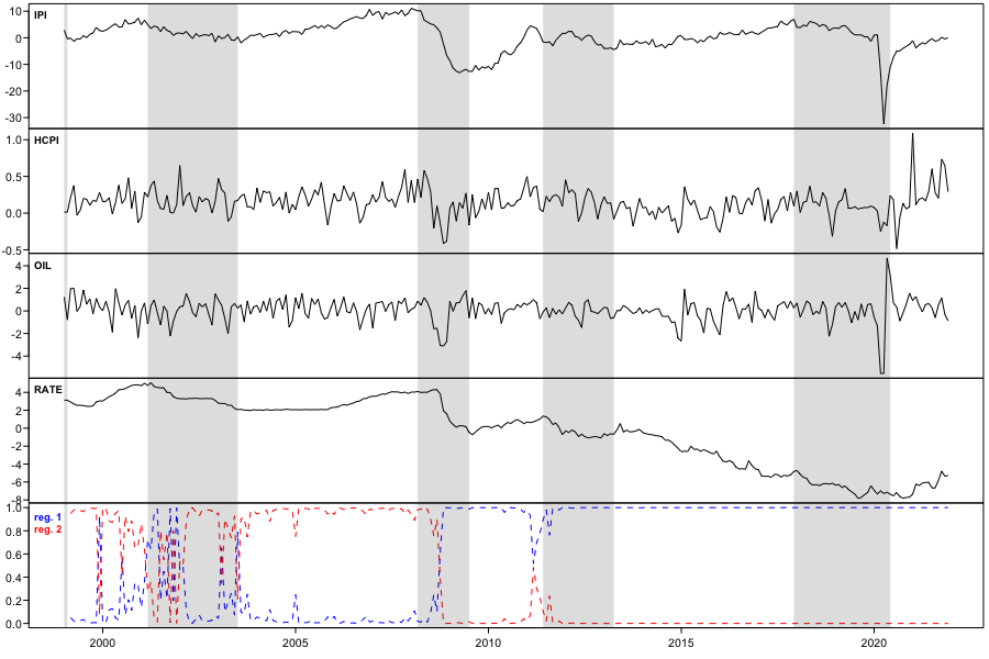
Figure 1: Monthly Euro area series covering the period from January 1999 to December 2021. The top panel presents the cyclical component of the industrial production index (IPI), which we separated from the trend using the linear projection filter proposed by Hamilton (2018). The second and third panels the log-differences of the harmonized consumer price index (HCPI) and Brent crude oil prices (Europe, OIL) multiplied by hundred and ten, respectively. The fourth panel presents an interest rate variable which is the EONIA from January 1999 to October 2008 and the Wu and Xia (2016) shadow rate from November 2008 to December 2021. The bottom panel shows the estimated mixing weights of the fitted StMVAR($2,2$) model. The shaded areas indicate the periods of Euro area recessions defined by the OECD.

For selecting the order our G-StMVAR model, we started by estimating one-regime StMVAR models with autoregressive orders $p=1,...,12$ and found that AIC was minimized by the order $p=1$. Then, we estimated a two-regime StMVAR model with $p=1$ but found this model somewhat inadequate. Therefore, we increased the autoregressive order to $p=2$, which increased the AIC. The overall adequacy of the StMVAR($2,2$) model, i.e., G-StMVAR($p=2$, $M_{1}=0$, $M_{2}=2$) model, was found reasonable, so we employ it for the further analysis. Because the model does not contain large degrees of freedom parameter estimates, we do not consider incorporating Gaussian mixture components by switching to a G-StMVAR model with $M_{1}>0$. Details on model selection and the adequacy of the selected model are provided in Appendix C.1.

The estimated mixing weights of the StMVAR($2,2$) model are presented in the bottom panel of Figure 1. The first regime (blue) mainly prevails after the Financial crisis in 2008, but it obtains large mixing weights also before and during the early 2000’s recession. The second regime (red) dominates when the first one does not, that is, mainly before the Financial crisis. After the Financial crisis, its mixing weights stay close to zero, excluding a short period before the early 2010’s recession, however. Since the prevailing regime starts switching sharply from the second to the first in October 2008, our model is consistent with the evidence that the ECB changed its reaction function after the bankruptcy of Lehman Brothers in September 2008 (Gerlach and Lewis, 2014).

Based on unconditional means (and marginal variances) of the regimes (presented in Table 2 in Appendix C.2), the post-Financial crisis regime is characterized by negative (but volatile) output gap as well as lower inflation, oil price inflation, and interest rate variable than the pre-Financial crisis regime, which is characterized by positive output gap. The post-Financial crisis regime also exhibits higher kurtosis and overall volatility than the pre-Financial crisis regime. Details on the characteristics of the regimes are discussed in Appendix C.2. For the ease of communication, we will refer to the first regime as the low-growth post-Financial crisis regime and the second regime as the high-growth pre-Financial crisis regime without explicitly reminding that the classification is not a strict one: both regimes obtain large mixing weights before and after the Financial crisis, while both regimes also prevail during expansions and recessions.

7.1 Identification of a monetary policy shock

Decomposing the covariance matrices of the reduced form StMVAR($2,2$) model as in (4.5) gives the following estimates for the structural parameters:

$$\hat{W}=\begin{bmatrix}\phantom{-}0.77\ (0.512)&-0.94\ (0.618)&\boldsymbol{1.82}\ (0.771)&-0.13\ (0.271)\\ -0.12\ (0.069)&\phantom{-}0.12\ (0.077)&\boldsymbol{0.17}\ (0.079)&\phantom{-}0.03\ (0.026)\\ \boldsymbol{-1.05}\ (0.447)&-0.39\ (0.482)&0.56\ (0.306)&\phantom{-}0.21\ (0.143)\\ \phantom{-}0.01\ (0.016)&-0.02\ (0.022)&0.02\ (0.030)&\boldsymbol{\phantom{-}0.50}\ (0.199)\\ \end{bmatrix},\ \ \hat{\lambda}_{2}=\begin{bmatrix}0.50\ (0.397)\\ 0.36\ (0.291)\\ 0.19\ (0.155)\\ 0.03\ (0.021)\\ \end{bmatrix},$$ (7.1)

where the ordering of the variables is $y_{t}=(IPI_{t},HCPI_{t},OIL_{t},RATE_{t})$, the estimates $\hat{\lambda}_{2i}$ are in decreasing order (which fixes an arbitrary ordering for the columns of $\hat{W}$), and approximate standard errors are given in parentheses next to the estimates. The estimates that deviate from zero by more than two times their approximate standard error are bolded. We assume that the $\lambda_{2i}$ are all distinct, i.e., Assumption 1.

The estimates and approximate standard errors in (7.1) show that the fourth shock is the only shock that moves the interest variable (also statistically) significantly at impact, while it is also the only shock that moves production to the opposite direction. Therefore, we deem it as the monetary policy shock. The fourth shock, however, appears to move inflation and oil price inflation to the same direction as the interest rate variable, which is contrary to many of the standard economic theories stating that an increase in the nominal interest rate should decrease inflation by decreasing aggregate demand (e.g., Galí, 2015, and the references therein).

The monetary policy shock is identified with Proposition 1 (Proposition 2 of Virolainen, 2022) by placing such constraints on $W$ (or equivalently the B-matrix) that it is unambiguously distinguished from the other shocks. We assume that the monetary policy shock moves the interest rate and production in opposite directions and that it does not move inflation nor oil price inflation at impact. The zero constraints on inflation and oil price inflation obtained the $p$-values $0.22$ and $0.15$ in a Wald test individually and the $p$-value $0.34$ jointly, so they are not rejected. These zero constraints are useful for distinguishing the monetary policy shock from the other shocks, but they also dampen the arguably implausible instantaneous increase in prices in response to a contractionary monetary policy shock. The monetary policy shock is distinguished from the other shocks by assuming that first shock moves oil price inflation at impact and that the second and third shocks move inflation at impact. This is not economically restrictive, as the responses can be very small. The obtained estimates and their approximate standard errors are presented in Appendix C.3.

7.2 Impulse response analysis

Following Virolainen (2022) (and others), we employ the generalized impulse response function (GIRF) (Koop et al., 1996) for estimating the expected effects of the monetary policy shocks. The GIRF is defined as

$$\text{GIRF}(h,\delta_{j},\mathcal{F}_{t-1})=\text{E}[y_{t+h}|\delta_{j},\mathcal{F}_{t-1}]-\text{E}[y_{t+h}|\mathcal{F}_{t-1}],$$ (7.2)

where $h\in\{0,1,2,...\}$ is the horizon and $\mathcal{F}_{t-1}=\sigma\{y_{t-j},j>0\}$ as before. The first term on the right side is the expected realization of the process at time $t+h$ conditionally on a structural shock of magnitude $\delta_{j}\in\mathbb{R}$ in the $j$th element of $e_{t}$ at time $t$ and the previous observations. The second term on the right side is the expected realization of the process conditionally on the previous observations only. The GIRF thus expresses the expected difference in the future outcomes when the structural shock of size $\delta_{j}$ in the $j$th element hits the system at time $t$ as opposed to all shocks being random. It is interesting to also study the effects of the monetary policy shock to the mixing weights $\alpha_{m,t}$ in which case $y_{t+h}$ is replaced with $\alpha_{m,t+h}$ on the right side of (7.2).

The G-StMVAR model has a $p$-step Markov property, so the GIRF can be calculated conditionally on the ($\sigma$-algebra generated by the) $p$ previous observations $\boldsymbol{y}_{t-1}=(y_{t-1},...,y_{t-p})$. We make use of this property by generating histories $\boldsymbol{y}_{t-1}=(y_{t-1},...,y_{t-p})$ from the stationary distribution of each regime separately, and thereby obtain GIRFs conditional on the starting values being from this regime. The GIRFs and confidence intervals that reflect uncertainty about the initial value within the given regime are estimated using the Monte Carlo algorithm presented in Virolainen (2022), where the point estimate is the mean over the Monte Carlo replication and the confidence intervals are obtained from the empirical quantiles.

The StMVAR model accommodates asymmetries in the GIRFs with respect the initial state of the economy as well as to the sign and size of the shock. We study these three types of asymmetries by generating starting values from each regime separately and then estimating GIRFs for positive (contractionary) and negative (expansionary) one-standard-error (small) and two-standard-error (large) shocks. After estimating the GIRFs, we scale them so that they correspond to a $25$ basis point instantaneous increase of the interest rate variable, making any asymmetries easy to detect.

Figure 2 presents the GIRFs $h=0,1,...,96$ months ahead estimated for the identified monetary policy shock. The GIRFs of inflation and oil price inflation are accumulated to (scaled) log-levels. From top to bottom, the responses of IPI, HCPI, oil price, interest rate, and the first regime’s mixing weights are depicted in each row, respectively. The first [third] column shows the responses to small contractionary (blue solid line) and expansionary (red dashed line) shocks with the initial values generated from the stationary distribution of the low-growth post-Financial crisis [high-growth pre-Financial crisis] regime. The second [fourth] column shows the responses to large contractionary and expansionary shocks with the initial values generated from the the low-growth post-Financial crisis [high-growth pre-Financial crisis] regime. The shaded areas are the $90\%$ confidence intervals that reflect the uncertainty about the initial value within the given regime. Responses of the second regime’s mixing weights are not depicted because they are the negative of those of the first regime.

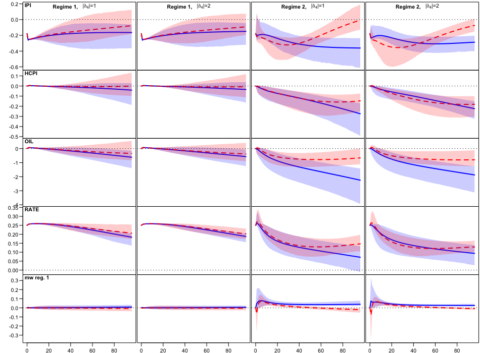
Figure 2: Generalized impulse response functions $h=0,1,....,96$ months ahead estimated for the monetary policy shock identified in Section 7.1 using $R_{1}=R_{2}=2500$ in the Monte Carlo algorithm presented in Virolainen (2022). From top to bottom, the responses of production, HCPI, oil price, the interest rate variable, and the first regime’s mixing weights are depicted in each row, respectively. The GIRFs of the HCPI and oil price are accumulated to (scaled) log-levels. The first [third] column shows the responses to one-standard-error contractionary (blue solid line) and expansionary (red dashed line) shocks with the initial values generated from the stationary distribution of the low-growth post-Financial crisis [high-growth pre-Financial crisis] regime. The second [fourth] column shows the responses to two-standard error contractionary and expansionary shocks with the initial values generated from the low-growth post-Financial crisis [high-growth pre-Financial crisis] regime. After estimation, all GIRFs were scaled so that the instantaneous movement of the interest rate variable is $25$ basis points. The shaded areas are the $90\%$ confidence intervals that reflect uncertainty about the initial state within the given regime. Responses of the second regime’s mixing weights are not depicted because they are the negative of those of the first regime.

In the low-growth post-Financial crisis regime (the first and second columns of Figure 2), the IPI decreases (increases) strongly at impact in response to a contractionary (expansionary) monetary policy shock. On average, the peak response is in the first period, and then the average response starts to slowly decay towards zero. The confidence intervals show that with some of the starting values the peak effect occurs later, however. The effects seem to die out faster for an expansionary than a contractionary shock.

In response to a contractionary shock, the average price level stays roughly at zero for several years but decreases slowly and persistently. In response to an expansionary shock, the price level barely moves on average in the horizon of eight years, but confidence bounds show that with some of the starting values it decreases and from some increases. The oil price seems to increase (decrease) slightly for roughly fifteen months before it decreases (increases) persistently. The confidence bounds, however, show that with some starting values the expansionary shock may decrease the oil price. The interest rate variable stays high (low) very persistently, and the GIRFs seem quite symmetric with respect to the size of the shock.

In the high-growth pre-Financial crisis regime (the third and fourth columns of Figure 2), the IPI decreases (increases) strongly at impact as a response to a contractionary (expansionary) monetary policy shock. On average, the response then decreases (increases) and peaks roughly after two and a half years for an expansionary shock, but stays low very persistently without a particular peak effect for a contractionary shock. The IPI stays low very persistently, because the probability of entering the low-growth post-Financial crisis regime stays above zero very persistently, as the responses of first regime’s mixing weights show (the bottom panels of the third and fourth columns in Figure 2).

The price level starts to steadily decrease (increase) after the impact period. The average price level somewhat stabilizes roughly after two years when the shock is expansionary, but keeps decreasing over our horizon of eight years when the shock is contractionary. The confidence bounds show that with some of the initial values, the price level decays towards zero after several years when the shock is small and expansionary. The oil price moves similarly to the consumer prices, whereas the interest rate variable stays high (low) persistently, more so if the shock is expansionary. Interestingly, an expansionary shock significantly increases the probability of the low-growth regime in the first period, but in the following periods it significantly increases the probability of the high-growth regime.

Overall, we find strong asymmetries with respect to the initial state of the economy and the sign of the shock, but the asymmetries are weak with respect to the size of the shock. The real effects are less enduring for an expansionary shock than for a contractionary shock. Particularly in the high-growth regime, a contractionary shock persistently drives the economy towards the low-growth regime, which translates to very persistent decrease in the output gap. The inflationary effects of the monetary policy shock are stronger in the high-growth regime, while they are on average weak in the low-growth regime. In the low-growth regime, however, monetary policy is mainly measured with the Wu and Xia (2016) shadow rate instead of EONIA, which is mostly close to zero after the Financial crisis. Thus, the outcome might differ in the two regimes also due to the different measures of monetary policy.

8 Summary

We introduced a new mixture vector autoregressive model, which has attractive theoretical and practical properties. The G-StMVAR model accommodates conditionally homoskedastic Gaussian VARs and conditionally heteroskedastic Student’s $t$ VARs as its mixture components. The mixing weights are defined as weighted ratios of the component process stationary densities corresponding to $p$ previous observations. Therefore, the greater the relative weighted likelihood of a regime is, the more likely the process is to generate an observation from it. This facilitates associating statistical characteristic and economic interpretations to the regimes. The specific formulation of the mixing weights also leads to attractive theoretical properties such as ergodicity and full knowledge of the stationary distribution of $p+1$ consecutive observations. Moreover, the maximum likelihood estimator of a stationary G-StMVAR model is strongly consistent, and therefore, it has the conventional limiting distribution under conventional high level conditions.

The G-StMVAR model is a multivariate version of the G-StMAR model of Virolainen (forthcoming). As special case, by assuming that all the mixture components are linear Student’s $t$ VARs, we also obtained a multivariate version of the StMAR model of Meitz et al. (forthcoming), which we call the StMVAR model. In addition to the reduced form model, we introduced a structural version of the G-StMVAR model with a time-varying impact matrix and statistically identified shocks. Referring to Virolainen (2022), we discussed the problem of identifying the structural shocks and presented a general set of conditions for identifying any subset of the shocks. We then employed the structural model in the empirical application. The accompanying CRAN distributed R package gmvarkit (Virolainen, 2018a) provides a comprehensive set of tools for maximum likelihood estimation and other numerical analysis of the introduced models.

The empirical application studied asymmetries in the expected effects of the monetary policy shock in the Euro area and considered a monthly data covering the period from January 1999 to December 2021. Our StMVAR model identified two regimes: a low-growth regime and a high-growth regime. The low-growth regime is characterized by a negative (but volatile) output gap, and it mainly prevails after the collapse of Lehman Brothers in the Financial crisis but obtains large mixing weights also during and before the early 2000’s recession. The high-growth regime is characterized by a positive output gap and it mainly dominates before the Financial crisis.

We found strong asymmetries with respect to the initial state of the economy and the sign of the shock, but asymmetries with respect to the size of the shock were weak. The real effects are less enduring for an expansionary shock than for a contractionary shock. Particularly in the high-growth pre-Financial crisis regime, a contractionary shock persistently drives the economy towards the low-growth post-Financial crisis regime, which translates to a very persistent decrease in the output gap. The inflationary effects of the monetary policy shock are stronger in the high-growth regime than in the low-growth regime, and in the latter the price level did not move much on average. In the low-growth regime, however, monetary policy is mainly measured with the Wu and Xia (2016) shadow rate instead of EONIA, which is mostly close to zero after the Financial crisis.

Appendix A Properties of multivariate Gaussian and Student’s t distribution

Denote a $d$-dimensional real valued vector by $y$. It is well known that the density function of a $d$-dimensional Gaussian distribution with mean $\mu$ and covariance matrix $\Sigma$ is

$$n_{d}(y;\mu,\Sigma)=(2\pi)^{-d/2}\text{det}(\Sigma)^{-1/2}\exp\left\{-\frac{1}{2}(y-\mu)^{\prime}\Sigma^{-1}(y-\mu)\right\}.$$ (A.1)

Similarly to Meitz et al. (forthcoming) but differing from the standard form, we parametrize the Student’s $t$-distribution using its covariance matrix as a parameter together with the mean and the degrees of freedom. The density function of such a $d$-dimensional $t$-distribution with mean $\mu$, covariance matrix $\Sigma$, and $\nu>2$ degrees of freedom is (see, e.g., Appendix A in Meitz et al., forthcoming)

$$t_{d}(y;\mu,\Sigma,\nu)=C_{d}(\nu)\text{det}(\Sigma)^{-1/2}\left(1+\frac{(y-\mu)^{\prime}\Sigma^{-1}(y-\mu)}{\nu-2}\right)^{-(d+\nu)/2},$$ (A.2)

where

$$C_{d}(\nu)=\frac{\Gamma\left(\frac{d+\nu}{2}\right)}{\sqrt{\pi^{d}(\nu-2)^{d}}\Gamma\left(\frac{\nu}{2}\right)},$$ (A.3)

and $\Gamma\left(\cdot\right)$ is the gamma function. We assume that the covariance matrix $\Sigma$ is positive definite for both distributions.

Consider a partition $X=(X_{1},X_{2})$ of either Gaussian or $t$-distributed (with $\nu$ degrees of freedom) random vector $X$ such that $X_{1}$ has dimension $(d_{1}\times 1)$ and $X_{2}$ has dimension $(d_{2}\times 1)$. Consider also a corresponding partition of the mean vector $\mu=(\mu_{1},\mu_{2})$ and the covariance matrix

$$\Sigma=\begin{bmatrix}\Sigma_{11}&\Sigma_{12}\\ \Sigma_{12}^{\prime}&\Sigma_{22}\end{bmatrix},$$ (A.4)

where, for example, the dimension of $\Sigma_{11}$ is $(d_{1}\times d_{1})$. In the Gaussian case, $X_{1}$ then has the marginal distribution $n_{d_{1}}(\mu_{1},\Sigma_{11})$ and $X_{2}$ has the marginal distribution $n_{d_{2}}(\mu_{2},\Sigma_{22})$. In the Student’s $t$ case, $X_{1}$ has the marginal distribution $t_{d_{1}}(\mu_{1},\Sigma_{11},\nu)$ and $X_{2}$ has the marginal distribution $t_{d_{2}}(\mu_{2},\Sigma_{22},\nu)$ (see, e.g., Ding (2016), also in what follows).

When $X$ has Gaussian distribution, the conditional distribution of the random vector $X_{1}$ given $X_{2}=x_{2}$ is

$$X_{1}\mid(X_{2}=x_{2})\sim n_{d_{1}}(\mu_{1\mid 2}(x_{2}),\Sigma_{1\mid 2}(x_{2})),$$ (A.5)

where

$$\mu(x_{2})\equiv\mu_{1\mid 2}(x_{2}) =\mu_{1}+\Sigma_{12}\Sigma_{22}^{-1}(x_{2}-\mu_{2})\quad\text{and}$$ (A.6)

$$\Omega\equiv\Sigma_{1\mid 2}(x_{2}) =\Sigma_{11}-\Sigma_{12}\Sigma_{22}^{-1}\Sigma_{12}^{\prime}.$$ (A.7)

When $X$ has $t$-distribution, the conditional distribution of the random vector $X_{1}$ given $X_{2}=x_{2}$ is

$$X_{1}\mid(X_{2}=x_{2})\sim t_{d_{1}}(\mu_{1\mid 2}(x_{2}),\Sigma_{1\mid 2}(x_{2}),\nu+d_{2}),$$ (A.8)

where

$$\mu(x_{2})=\mu_{1\mid 2}(x_{2}) =\mu_{1}+\Sigma_{12}\Sigma_{22}^{-1}(x_{2}-\mu_{2})\quad\text{and}$$ (A.9)

$$\Omega(x_{2})\equiv\Sigma_{1\mid 2}(x_{2}) =\frac{\nu-2+(x_{2}-\mu_{2})^{\prime}\Sigma_{22}^{-1}(x_{2}-\mu_{2})}{\nu-2+d_{2}}(\Sigma_{11}-\Sigma_{12}\Sigma_{22}^{-1}\Sigma_{12}^{\prime}).$$ (A.10)

In particular, we have

$$n_{d}(x;\mu,\Sigma) =n_{d_{1}}(x_{1};\mu_{1|2}(x_{2}),\Sigma_{1|2}(x_{2}))n_{d_{2}}(x_{2};\mu_{2},\Sigma_{22})\quad\text{and}$$ (A.11)

$$t_{d}(x;\mu,\Sigma,\nu) =t_{d_{1}}(x_{1};\mu_{1|2}(x_{2}),\Sigma_{1|2}(x_{2}),\nu+d_{2})t_{d_{2}}(x_{2};\mu_{2},\Sigma_{22},\nu).$$ (A.12)

Appendix B Proofs

B.1 Proof of Theorem 1

Corresponding to $\phi_{0}\in\mathbb{R}^{d}$, $\boldsymbol{A}_{p}\in\mathbb{S}^{d\times dp}$, $\Omega\in\mathbb{R}^{d\times d}$ positive definite, and $\nu>2$, define the notation $\mu$, $\Sigma_{p}$, $\Sigma_{1}(h)$ $(h=0,1,...,p)$, $\Sigma_{1p}$, and $\Sigma_{p+1}$ as in (2.4)-(2.6). Note that by construction and the assumption $\boldsymbol{A}_{p}\in\mathbb{S}^{d\times dp}$, $\Sigma_{p}$ and $\Sigma_{p+1}$ are symmetric positive definite block Toeplitz matrices with the $(d\times d)$ blocks $\Sigma_{1}(h)$, $h=0,1,...,p$. Analogously to Meitz et al. (forthcoming), we prove Part 2.9 by constructing a $dp$-dimensional Markov chain $\boldsymbol{z}_{t}=(z_{t},...,z_{t-p+1})$ ($t=1,2,...$) with the desired properties. Then, we make use of the theory of Markov chains to establish its stationary distribution. To that end, an appropriate transition probability measure and an initial distribution needs to be specified. For the former, assume that the transition probability of $\boldsymbol{z}_{t}$ is determined by the density function $t_{d}(z_{t};\mu(\boldsymbol{z}_{t-1}),\Omega(\boldsymbol{z}_{t-1}),\nu+dp)$, where $\mu(\boldsymbol{z}_{t-1})$ and $\Omega(\boldsymbol{z}_{t-1})$ are obtained from (A.9) and (A.10), respectively, by replacing $\boldsymbol{x}_{2}$ with $\boldsymbol{z}_{t-1}$. Because the distribution of the current observation depends only on the previous one, $\boldsymbol{z}_{t}$ is a Markov chain on $\mathbb{R}^{dp}$.

Suppose the initial value $\boldsymbol{z}_{0}$ follows the $t$-distribution $t_{dp}(\boldsymbol{1}_{p}\otimes\mu,\Sigma_{p},\nu)$. The properties of $t$-distribution (given in Appendix A) then imply that if $\boldsymbol{z}_{t}^{+}=(z_{t},\boldsymbol{z}_{t-1})$, the density function of $\boldsymbol{z}_{1}^{+}$ is given by

$$t_{d(p+1)}(\boldsymbol{z}_{1}^{+};\boldsymbol{1}_{p+1}\otimes\mu,\Sigma_{p+1},\nu)=t_{d}(z_{1};\mu(\boldsymbol{z}_{0}),\Omega(\boldsymbol{z}_{0}),\nu+dp)t_{dp}(\boldsymbol{z}_{0};\boldsymbol{1}_{p}\otimes\mu,\Sigma_{p},\nu).$$ (B.1)

Thus, $\boldsymbol{z}_{1}^{+}\sim t_{d(p+1)}(\boldsymbol{1}_{p+1}\otimes\mu,\Sigma_{p+1},\nu)$, and from the block Toeplitz structure of $\Sigma_{p+1}$ it follows that the marginal distribution of $\boldsymbol{z}_{1}$ is the same as that of $\boldsymbol{z}_{0}$, i.e., $\boldsymbol{z}_{1}\sim t_{dp}(\boldsymbol{1}_{p}\otimes\mu,\Sigma_{p},\nu)$. Hence, as $\boldsymbol{z}_{t}$ is a Markov chain, it has a stationary distribution characterized by the density $t_{dp}(\boldsymbol{1}_{p}\otimes\mu,\Sigma_{p},\nu)$ (Meyn and Tweedie, 2009, pp. 230-231), completing the proof of Part 2.9.

Denote by $\mathcal{F}_{t-1}^{z}$ the $\sigma$-algebra generated by the random variables $\{z_{s},s<t\}$. To prove Part 2.10, note that due to the Markov property, $z_{t}|\mathcal{F}_{t-1}^{z}\sim t_{d}(\mu(\boldsymbol{z}_{0}),\Omega(\boldsymbol{z}_{0}),\nu+dp)$. Therefore, the conditional expectation and conditional variance of $z_{t}$ given $\mathcal{F}_{t-1}^{z}$ can be written as

$$E[z_{t}|\mathcal{F}_{t-1}^{z}]= E[z_{t}|\boldsymbol{z}_{t-1}]=\mu+\Sigma_{1p}\Sigma_{p}^{-1}(\boldsymbol{z}_{t-1}-\boldsymbol{1}_{p}\otimes\mu)=\phi_{0}+\boldsymbol{A}_{p}\boldsymbol{z}_{t-1},$$ (B.2)

$$Var[z_{t}|\mathcal{F}_{t-1}^{z}]= Var[z_{t}|\boldsymbol{z}_{t-1}]=\frac{\nu-2+(\boldsymbol{z}_{t-1}-\boldsymbol{1}_{p}\otimes\mu)^{\prime}\Sigma_{p}^{-1}(\boldsymbol{z}_{t-1}-\boldsymbol{1}_{p}\otimes\mu)}{\nu-2+dp}\Omega,$$ (B.3)

where $\Omega=\Sigma_{1}-\Sigma_{1p}\Sigma_{p}^{-1}\Sigma_{1p}^{\prime}$. We denote this conditional variance by $\Omega_{t}\equiv\Omega(\boldsymbol{z}_{t-1})$, which is positive definite due to the assumptions $\nu>2$ and that $\Sigma_{p}$ and $\Omega$ are both positive definite. Define the $(d\times 1)$ random vectors $\varepsilon_{t}$ as

$$\varepsilon_{t}\equiv\Omega_{t}^{-1/2}(z_{t}-\phi_{0}-\boldsymbol{A}_{p}\boldsymbol{z}_{t-1}),$$ (B.4)

where $\Omega_{t}^{-1/2}$ is a symmetric square root matrix of $\Omega_{t}^{-1}$. Conditionally on $\mathcal{F}_{t-1}^{z}$, $\varepsilon_{t}$ now follow the $t_{d}(0,I_{d},\nu+dp)$ distribution, and therefore the ’VAR($p$)-ARCH($p$)’ representation (2.10) is obtained. Because this conditional distribution does not depend on $\mathcal{F}_{t-1}^{z}$, it follows that the unconditional distribution of $\varepsilon_{t}$ is also $t_{d}(0,I_{d},\nu+dp)$. Hence, $\varepsilon_{t}$ is independent of $\mathcal{F}_{t-1}^{z}$ (or of $\{z_{s},s<t\}$), and as the random vectors $\{\varepsilon_{s},s<t\}$ are functions of $\{z_{s},s<t\}$, $\varepsilon_{t}$ is also independent of $\{\varepsilon_{s},s<t\}$. Thus, the proof of Part 2.10 is completed by concluding that the random vectors $\varepsilon_{t}$ are IID $t_{d}(0,I_{d},\nu+dp)$ distributed.$\blacksquare$

B.2 Proof of Theorem 2

The G-StMVAR process $\boldsymbol{y}_{t}$ is clearly a Markov chain on $\mathbb{R}^{dp}$. Let $\boldsymbol{y}_{0}=(y_{0},...,y_{-p+1})$ be random vector whose distribution is characterized by the density $f(\boldsymbol{y}_{0};\boldsymbol{\theta})=\sum_{m=1}^{M_{1}}\alpha_{m}n_{dp}(\boldsymbol{y}_{0};\boldsymbol{1}_{p}\otimes\mu_{m},\Sigma_{m,p})+\sum_{m=M_{1}+1}^{M}\alpha_{m}t_{dp}(\boldsymbol{y}_{0};\boldsymbol{1}_{p}\otimes\mu_{m},\Sigma_{m,p},\nu_{m})$. According to (2.3), (3.1), (3.5), and (B.1), the conditional density of $y_{1}$ given $\boldsymbol{y}_{0}$ is

$$f(y_{1}|\boldsymbol{y}_{0};\boldsymbol{\theta})= \sum_{m=1}^{M_{1}}\frac{\alpha_{m}n_{dp}(\boldsymbol{y}_{0};\boldsymbol{1}_{p}\otimes\mu_{m},\Sigma_{m,p})}{f(\boldsymbol{y}_{0};\boldsymbol{\theta})}n_{d}(y_{1};\mu_{m,1}(\boldsymbol{y}_{0}),\Omega_{m,1})$$

$$+\sum_{m=M_{1}+1}^{M}\frac{\alpha_{m}t_{dp}(\boldsymbol{y}_{0};\boldsymbol{1}_{p}\otimes\mu_{m},\Sigma_{m,p},\nu_{m})}{f(\boldsymbol{y}_{0};\boldsymbol{\theta})}t_{d}(y_{1};\mu_{m,1}(\boldsymbol{y}_{0}),\Omega_{m,1}(\boldsymbol{y}_{0}),\nu_{m}+dp)$$ (B.5)

$$= \sum_{m=1}^{M_{1}}\frac{\alpha_{m}}{f(\boldsymbol{y}_{0};\boldsymbol{\theta})}n_{d(p+1)}((y_{t},\boldsymbol{y}_{0});\boldsymbol{1}_{p+1}\otimes\mu_{m},\Sigma_{m,p+1})$$

$$+\sum_{m=M_{1}+1}^{M}\frac{\alpha_{m}}{f(\boldsymbol{y}_{0};\boldsymbol{\theta})}t_{d(p+1)}((y_{t},\boldsymbol{y}_{0});\boldsymbol{1}_{p+1}\otimes\mu_{m},\Sigma_{m,p+1},\nu_{m}).$$ (B.6)

The random vector $(y_{1},\boldsymbol{y}_{0})$ therefore has the density

$$\begin{aligned} f(y_{1},\boldsymbol{y}_{0})=&\sum_{m=1}^{M_{1}}\alpha_{m}n_{d(p+1)}((y_{1},\boldsymbol{y}_{0});\boldsymbol{1}_{p+1}\otimes\mu_{m};\Sigma_{m,p+1})\\ &+\sum_{m=M_{1}+1}^{M}\alpha_{m}t_{d(p+1)}((y_{1},\boldsymbol{y}_{0});\boldsymbol{1}_{p+1}\otimes\mu_{m};\Sigma_{m,p+1},\nu_{m}).\end{aligned}$$ (B.7)

Integrating $y_{-p+1}$ out, and using the properties of marginal distributions of a multivariate Gaussian and $t$-distributions (see Appendix A) together with the block Toeplitz form of $\Sigma_{m,p+1}$ shows that the density of $\boldsymbol{y}_{1}$ is $f(\boldsymbol{y}_{1};\boldsymbol{\theta})=\sum_{m=1}^{M_{1}}\alpha_{m}n_{dp}(\boldsymbol{y}_{1};\boldsymbol{1}_{p}\otimes\mu_{m},\Sigma_{m,p})+\sum_{m=M_{1}+1}^{M}\alpha_{m}t_{dp}(\boldsymbol{y}_{1};\boldsymbol{1}_{p}\otimes\mu_{m},\Sigma_{m,p},\nu_{m})$. Thus, $\boldsymbol{y}_{0}$ and $\boldsymbol{y}_{1}$ are identically distributed. As $\{\boldsymbol{y}_{t}\}_{t=1}^{\infty}$ is a (time-homogeneous) Markov chain, it follows that $\{\boldsymbol{y}_{t}\}_{t=1}^{\infty}$ has a stationary distribution, say $\pi_{\boldsymbol{y}}(\cdot)$, characterized by the density $f(\cdot;\boldsymbol{\theta})=\sum_{m=1}^{M_{1}}\alpha_{m}n_{dp}(\cdot;\boldsymbol{1}_{p}\otimes\mu_{m},\Sigma_{m,p})+\sum_{m=M_{1}+1}^{M}\alpha_{m}t_{dp}(\cdot;\boldsymbol{1}_{p}\otimes\mu_{m},\Sigma_{m,p},\nu_{m})$ (Meyn and Tweedie, 2009, pp. 230-231).

For ergodicity, let $P_{\boldsymbol{y}}(\boldsymbol{y},\cdot)=\mathbb{P}(\boldsymbol{y}_{p}\in\cdot|\boldsymbol{y}_{0}=\boldsymbol{y})$ signify the $p$-step transition probability measure of the process $\boldsymbol{y}_{t}$. Using the $p$th order Markov property of $y_{t}$, it is straightforward to check that $P_{\boldsymbol{y}}(\boldsymbol{y},\cdot)$ has the density

$$\begin{aligned} &f(\boldsymbol{y}_{p}|\boldsymbol{y}_{0};\boldsymbol{\theta})=\prod_{t=1}^{p}f(y_{t}|\boldsymbol{y}_{t-1};\boldsymbol{\theta})=\\ &\prod_{t=1}^{p}\left(\sum_{m=1}^{M_{1}}\alpha_{m}n_{d}(y_{1};\mu_{m,t}(\boldsymbol{y}_{t-1}),\Omega_{m})+\sum_{m=M_{1}+1}^{M}\alpha_{m}t_{d}(y_{1};\mu_{m,t}(\boldsymbol{y}_{t-1}),\Omega_{m,t}(\boldsymbol{y}_{t-1}),\nu_{m}+dp)\right).\end{aligned}$$ (B.8)

Clearly, $f(\boldsymbol{y}_{p}|\boldsymbol{y}_{0};\boldsymbol{\theta})>0$ for all $\boldsymbol{y}_{0}\in\mathbb{R}^{dp}$ and $\boldsymbol{y}_{p}\in\mathbb{R}^{dp}$, so it can be concluded that $\boldsymbol{y}_{t}$ is ergodic in the sense of (Meyn and Tweedie, 2009, Chapter 13) by using arguments identical to those used in the proof of Theorem 1 in Kalliovirta et al. (2015).$\blacksquare$

B.3 Proof of Theorem 3

First note that $L_{T}^{(c)}(\boldsymbol{\theta})$ is continuous and that together with Assumption 2 it implies existence of a measurable maximizer $\hat{\boldsymbol{\theta}}_{T}$. To conclude that $\hat{\boldsymbol{\theta}}_{T}$ is strongly consistent, we need to show that (see, e.g., Newey and McFadden, 1994, Theorem 2.1 and the discussion on page 2122)

1. the uniform strong law of large numbers holds for the log-likelihood function; that is,
   

   $$\underset{\boldsymbol{\theta}\in\boldsymbol{\Theta}}{\sup}\left|L_{T}^{(c)}(\boldsymbol{\theta})-E[L_{T}^{(c)}(\boldsymbol{\theta})]\right|\rightarrow 0\quad\text{almost surely as}\quad T\rightarrow\infty,$$

2. and that the limit of $L_{T}^{(c)}(\boldsymbol{\theta})$ is uniquely maximized at $\boldsymbol{\theta}=\boldsymbol{\theta}_{0}$.

Proof of (i). By Theorem 2, the process $\boldsymbol{y}_{t-1}=(y_{t},...,y_{t-p+1})$, and hence also $y_{t}$, is stationary and ergodic, and $E[L_{T}^{(c)}(\boldsymbol{\theta})]=E[l_{t}(\boldsymbol{\theta})]$. To conclude (i), it therefore suffices to show that $E[\sup_{\boldsymbol{\theta}\in\boldsymbol{\Theta}}|l_{t}(\boldsymbol{\theta})|]<\infty$ (see Ranga Rao, 1962). We will do that by making use of the compactness of the parameter space to derive finite lower and upper bounds for $l_{t}(\boldsymbol{\theta})$, which is given as

$$l_{t}(\boldsymbol{\theta})=\log\left(\sum_{m=1}^{M_{1}}\alpha_{m,t}n_{d}(y_{t};\mu_{m,t},\Omega_{m})+\sum_{m=M_{1}+1}^{M}\alpha_{m,t}t_{d}(y_{t};\mu_{m,t},\Omega_{m,t},\nu_{m}+dp)\right).$$ (B.9)

First, we derive an upper bound for the normal distribution densities. Determinant of the positive definite conditional covariance matrix $\Omega_{m}$ is a continuous function of the parameters $vech(\Omega_{m})$, and hence, compactness of the parameter space implies that the determinant is bounded from below by some constant that is strictly larger than zero and from above by some finite constant. Thus,

$$0<c_{1}\leq\det(\Omega_{m})^{-1/2}\leq c_{2}<\infty,$$ (B.10)

for some constants $c_{1}$ and $c_{2}$. Because $\Omega_{m}^{-1}$ is positive definite and exponential function is bounded from above by one in the non-positive real axis, we obtain the upper bound

$$n_{d}(y_{t};\mu_{m,t},\Omega_{m})=(2\pi)^{-d/2}\text{det}(\Omega_{m})^{-1/2}\exp\left\{-\frac{1}{2}(y_{t}-\mu_{m})^{\prime}\Omega_{m}^{-1}(y_{t}-\mu_{m})\right\}\leq(2\pi)^{-d/2}c_{2}.$$ (B.11)

Next, we derive an upper bound for the $t$-distribution densities

$$\begin{aligned} t_{d}(y_{t};\mu_{m,t},\Omega_{m,t},\nu_{m}+dp)=&\frac{\Gamma\left(\frac{\nu_{m}+(1+p)d}{2}\right)}{\sqrt{\pi^{d}(\nu_{m}+dp-2)^{d}}\Gamma\left(\frac{\nu_{m}+dp}{2}\right)}\det(\Omega_{m,t})^{-1/2}\\ &\times\left(1+\frac{(y_{t}-\mu_{m,t})^{\prime}\Omega_{m,t}^{-1}(y_{t}-\mu_{m,t})}{\nu_{m}+dp-2}\right)^{-(\nu_{m}+d(1+p))/2}.\end{aligned}$$ (B.12)

Since $\nu_{m}>2$ and the parameter space is compact, $2<c_{3}\leq\nu_{m}\leq c_{4}<\infty$ for some constants $c_{3}$ and $c_{4}$. Because the gamma function is continuous on the positive real axis, it then follows that

$$0<c_{5}\leq\frac{\Gamma\left(\frac{\nu_{m}+(1+p)d}{2}\right)}{\sqrt{\pi^{d}(\nu_{m}+dp-2)^{d}}\Gamma\left(\frac{\nu_{m}+dp}{2}\right)}\leq c_{6}$$ (B.13)

for some finite constants $c_{5}$ and $c_{6}$.

Using the bounds $2<c_{3}\leq\nu_{m}\leq c_{4}<\infty$ and (B.10) together with the fact that $\Sigma_{m,p}^{-1}$ is positive definite gives

$$\begin{aligned} \det(\Omega_{m,t})^{-1/2}&=\left(\frac{\nu_{m}-2+(\boldsymbol{y}_{t-1}-\boldsymbol{1}_{p}\otimes\mu_{m})^{\prime}\Sigma_{m,p}^{-1}(\boldsymbol{y}_{t-1}-\boldsymbol{1}_{p}\otimes\mu_{m})}{\nu_{m}-2+dp}\right)^{-d/2}\det(\Omega_{m})^{-1/2}\\ &\leq\left(\frac{c_{3}-2}{c_{4}+dp-2}\right)^{-d/2}c_{2}<\infty.\end{aligned}$$ (B.14)

For a lower bound, note that $\Sigma_{m,p}^{-1}$ is a continuous function of the parameters and thereby its eigenvalues are as well. It then follows from the compactness of the parameter space that its largest eigenvalue, $\lambda_{1}^{max}$, is bounded from above by some finite constant, say $c_{7}$. The compactness of the parameter space also implies that there exist finite constant $c_{8}$ such that $\mu_{im}\leq c_{8}$ for all $i=1,..,d$ (where $\mu_{im}$ is the $i$th element of $\mu_{m}$). By using the orthonormal spectral decomposition of $\Sigma_{m,p}^{-1}$, we then obtain

$$\begin{aligned} (\boldsymbol{y}_{t-1}-\boldsymbol{1}_{p}\otimes\mu_{m})^{\prime}\Sigma_{m,p}^{-1}(\boldsymbol{y}_{t-1}-\boldsymbol{1}_{p}\otimes\mu_{m})&\leq\lambda_{1}^{max}(\boldsymbol{y}_{t-1}-\boldsymbol{1}_{p}\otimes\mu_{m})^{\prime}(\boldsymbol{y}_{t-1}-\boldsymbol{1}_{p}\otimes\mu_{m})\\ &\leq c_{7}(\boldsymbol{y}_{t-1}^{\prime}\boldsymbol{y}_{t-1}-2c_{8}\boldsymbol{y}_{t-1}^{\prime}\boldsymbol{1}_{dp}+dpc_{8}^{2}).\end{aligned}$$ (B.15)

Thus,

$$\det(\Omega_{m,t})^{-1/2}\geq\left(\frac{c_{4}-2+c_{7}(\boldsymbol{y}_{t-1}^{\prime}\boldsymbol{y}_{t-1}-2c_{8}\boldsymbol{y}_{t-1}^{\prime}\boldsymbol{1}_{dp}+dpc_{8}^{2})}{c_{3}-2+dp}\right)^{-d/2}c_{1}.$$ (B.16)

As $-(\nu_{m}+(1+p)d)/2<0$ and $\Omega_{m,t}^{-1}$ is positive definite, we have that

$$\left(1+\frac{(y_{t}-\mu_{m,t})^{\prime}\Omega_{m,t}^{-1}(y_{t}-\mu_{m,t})}{\nu_{m}+dp-2}\right)^{-(\nu_{m}+(1+p)d)/2}\leq 1.$$ (B.17)

Hence, $t_{d}(y_{t};\mu_{m,t},\Omega_{m,t},\nu_{m}+dp)\leq\left(\frac{c_{3}-2}{c_{4}+dp-2}\right)^{-d/2}c_{2}c_{6}$. It then follows from $\sum_{m=1}^{M}\alpha_{m,t}=1$ that

$$l_{t}(\boldsymbol{\theta})\leq\log\left(\max\left\{(2\pi)^{-d/2}c_{2},\left(\frac{c_{3}-2}{c_{4}+dp-2}\right)^{-d/2}c_{2}c_{6}\right\}\right)<\infty.$$ (B.18)

That is, $l_{t}(\boldsymbol{\theta})$ is bounded from above by a finite constant.

Next, we proceed by bounding $l_{t}(\boldsymbol{\theta})$ from below. Since the eigenvalues of $\Omega_{m}^{-1}$ are continuous functions of the parameters bounded by compactness of the parameter space, the largest eigenvalue, $\lambda_{2}^{max}$, is bounded from above by some finite constant, say $c_{9}$. Making use of the orthonormal spectral decomposition of $\Omega_{m}^{-1}$, we then obtain

$$\begin{aligned} (y_{t}-\mu_{m,t})^{\prime}\Omega_{m}^{-1}(y_{t}-\mu_{m,t})&\leq\lambda_{2}^{max}(y_{t}-\boldsymbol{A}_{m,p}\boldsymbol{y}_{t-1})^{\prime}(y_{t}-\boldsymbol{A}_{m,p}\boldsymbol{y}_{t-1})\\ &\leq c_{9}(y_{t}^{\prime}y_{t}-2y_{t}^{\prime}\boldsymbol{A}_{m,p}\boldsymbol{y}_{t-1}+\boldsymbol{y}_{t-1}^{\prime}\boldsymbol{A}_{m,p}^{\prime}\boldsymbol{A}_{m,p}\boldsymbol{y}_{t-1}).\end{aligned}$$ (B.19)

The compactness of the parameter space implies that

$$\boldsymbol{y}_{t-1}^{\prime}\boldsymbol{A}_{m,p}^{\prime}\boldsymbol{A}_{m,p}\boldsymbol{y}_{t-1}\leq c_{10}\sum_{i=1}^{dp}\sum_{j=1}^{dp}|\boldsymbol{y}_{j,t-1}\boldsymbol{y}_{i,t-1}|$$ (B.20)

for some finite constant $c_{10}$, where $\boldsymbol{y}_{i,t-1}$ is the $i$th element of $\boldsymbol{y}_{t-1}$. Denoting by $a_{m,i}(k,j)$ the $kj$th element of the autoregression matrix $A_{m,i}$ and $y_{kt}$ the $k$th element of $y_{t}$, we have

$$y_{t}^{\prime}\boldsymbol{A}_{m,p}\boldsymbol{y}_{t-1}=\sum_{k=1}^{d}\sum_{i=1}^{p}\sum_{j=1}^{d}a_{m,i}(k,j)y_{kt}y_{jt-i}\leq\sum_{k=1}^{d}\sum_{i=1}^{p}\sum_{j=1}^{d}c_{11}|y_{kt}y_{jt-i}|,$$ (B.21)

where $c_{11}$ is a finite constant that bounds the absolute values of the autoregression coefficients from above (which exists due to compactness of the parameter space). Combining the above two bounds with (B.19) gives the upper bound

$$(y_{t}-\mu_{m,t})^{\prime}\Omega_{m}^{-1}(y_{t}-\mu_{m,t})\leq c_{12}\left(y_{t}^{\prime}y_{t}+\sum_{i=1}^{dp}\sum_{j=1}^{dp}|\boldsymbol{y}_{j,t-1}\boldsymbol{y}_{i,t-1}|+\sum_{k=1}^{d}\sum_{i=1}^{p}\sum_{j=1}^{d}|y_{kt}y_{jt-i}|\right).$$ (B.22)

where $c_{12}$ is a finite constant.

Using the fact that $\Sigma_{m,p}^{-1}$ is positive definite together with the bounds $2<c_{3}\leq\nu_{m}\leq c_{4}<\infty$ shows that

$$\begin{aligned} \Omega_{m,t}^{-1}&=\frac{\nu_{m}-2+dp}{\nu_{m}-2+(\boldsymbol{y}_{t-1}-\boldsymbol{1}_{p}\otimes\mu_{m})^{\prime}\Sigma_{m,p}^{-1}(\boldsymbol{y}_{t-1}-\boldsymbol{1}_{p}\otimes\mu_{m})}\Omega_{m}^{-1}\leq\frac{c_{4}-2+dp}{c_{3}-2}\Omega_{m}^{-1}.\end{aligned}$$ (B.23)

Using the above inequality together with $2<c_{3}\leq\nu_{m}$ and (B.22) then gives

$$\frac{(y_{t}-\mu_{m,t})^{\prime}\Omega_{m,t}^{-1}(y_{t}-\mu_{m,t})}{v_{m}+pd-2}\leq c_{13}\left(y_{t}^{\prime}y_{t}+\sum_{i=1}^{dp}\sum_{j=1}^{dp}|\boldsymbol{y}_{j,t-1}\boldsymbol{y}_{i,t-1}|+\sum_{k=1}^{d}\sum_{i=1}^{p}\sum_{j=1}^{d}|y_{kt}y_{jt-i}|\right),$$ (B.24)

where $c_{13}=((c_{3}-2)(c_{3}+pd-2))^{-1}(c_{4}-2+dp)c_{12}$ is a finite constant.

From $\sum_{m=1}^{M}\alpha_{m,t}=1$, (B.10), (B.13), (B.16), (B.22), (B.24), and $\nu_{m}\leq c_{4}$, we then obtain a lower bound for $l_{t}(\boldsymbol{\theta})$ as

$$\begin{aligned} l_{t}(\boldsymbol{\theta})\geq\min&\left\{-\frac{d}{2}\log(2\pi)+\log(c_{1})\right.\\ &-\frac{1}{2}c_{12}\left(y_{t}^{\prime}y_{t}+\sum_{i=1}^{dp}\sum_{j=1}^{dp}|\boldsymbol{y}_{j,t-1}\boldsymbol{y}_{i,t-1}|+\sum_{k=1}^{d}\sum_{i=1}^{p}\sum_{j=1}^{d}|y_{kt}y_{jt-i}|\right),\\ &c_{15}-\frac{d}{2}\log(c_{4}-2+c_{7}(\boldsymbol{y}_{t-1}^{\prime}\boldsymbol{y}_{t-1}-2c_{8}\boldsymbol{y}_{t-1}^{\prime}\boldsymbol{1}_{dp}+dpc_{8}^{2}))\\ &\left.-c_{14}\log\left(1+c_{13}\left(y_{t}^{\prime}y_{t}+\sum_{i=1}^{dp}\sum_{j=1}^{dp}|\boldsymbol{y}_{j,t-1}\boldsymbol{y}_{i,t-1}|+\sum_{k=1}^{d}\sum_{i=1}^{p}\sum_{j=1}^{d}|y_{kt}y_{jt-i}|\right)\right)\right\},\end{aligned}$$ (B.25)

where $c_{14}=(c_{4}+(1+p)d)/2$ and $c_{15}=\log(c_{5})+\log(c_{1})+\frac{d}{2}(c_{3}-2+dp)$. Since $y_{t}$ is stationary with finite second moments, it holds that

$$\begin{aligned} &E\left[y_{t}^{\prime}y_{t}+\sum_{i=1}^{dp}\sum_{j=1}^{dp}|\boldsymbol{y}_{j,t-1}\boldsymbol{y}_{i,t-1}|+\sum_{k=1}^{d}\sum_{i=1}^{p}\sum_{j=1}^{d}|y_{kt}y_{jt-i}|\right]<\infty\ \ \text{and}\\ &E[\boldsymbol{y}_{t-1}^{\prime}\boldsymbol{y}_{t-1}-2c_{8}\boldsymbol{y}_{t-1}^{\prime}\boldsymbol{1}_{dp}]<\infty,\end{aligned}$$ (B.26)

and thereby we obtain from Jensen’s inequality that also

$$\begin{aligned} &E\left[\log\left(1+c_{13}\left(y_{t}^{\prime}y_{t}+\sum_{i=1}^{dp}\sum_{j=1}^{dp}|\boldsymbol{y}_{j,t-1}\boldsymbol{y}_{i,t-1}|+\sum_{k=1}^{d}\sum_{i=1}^{p}\sum_{j=1}^{d}|y_{kt}y_{jt-i}|\right)\right)\right]<\infty\ \ \text{and}\\ &E[\log(c_{4}-2+c_{7}(\boldsymbol{y}_{t-1}^{\prime}\boldsymbol{y}_{t-1}-2c_{8}\boldsymbol{y}_{t-1}^{\prime}\boldsymbol{1}_{dp}+dpc_{8}^{2}))]<\infty.\end{aligned}$$ (B.27)

The upper bound (B.18) together with (B.25), (B.26), and (B.27) shows that $E[\sup_{\boldsymbol{\theta}\in\boldsymbol{\Theta}}|l_{t}(\boldsymbol{\theta})|]<\infty$.$\blacksquare$

Proof of (ii). To prove that $E[l_{t}(\boldsymbol{\theta})]$ is uniquely maximized at $\boldsymbol{\theta}=\boldsymbol{\theta}_{0}$, it needs to be shown that $E[l_{t}(\boldsymbol{\theta})]\leq E[l_{t}(\boldsymbol{\theta}_{0})]$, and that $E[l_{t}(\boldsymbol{\theta})]=E[l_{t}(\boldsymbol{\theta}_{0})]$ implies

$$\begin{aligned} &\boldsymbol{\vartheta}_{m}=\boldsymbol{\vartheta}_{\tau(m),0}\ \ \text{and}\ \ \alpha_{m}=\alpha_{\tau(m),0}\ \ \text{when}\ \ m=1,....,M_{1},\ \ \text{and}\\ &(\boldsymbol{\vartheta}_{m},\nu_{m})=(\boldsymbol{\vartheta}_{\tau(m),0},\nu_{\tau(m),0})\ \ \text{and}\ \ \alpha_{m}=\alpha_{\tau(m),0}\ \ \text{when}\ \ m=M_{1}+1,....,M,\end{aligned}$$ (B.28)

for some permutations $\{\tau_{1}(1),...,\tau_{1}(M_{1})\}$ and $\{\tau_{2}(M_{1}+1),...,\tau_{2}(M)\}$. For notational clarity, we write $\mu_{m,t}=\mu(\boldsymbol{y};\boldsymbol{\vartheta}_{m})$, $\Omega_{m}=\Omega(\boldsymbol{\vartheta}_{m})$, $\Omega_{m,t}=\Omega(\boldsymbol{y};\boldsymbol{\vartheta}_{m},\nu_{m})$, and $\alpha_{m,t}=\alpha_{m}(\boldsymbol{y};\boldsymbol{\theta})$, making clear their dependence on the parameter value.

The density of $(y_{t},\boldsymbol{y}_{t-1})$ can be written as

$$\begin{aligned} f((y_{t},\boldsymbol{y}_{t-1});\boldsymbol{\theta}_{0})=&\sum_{n=1}^{M}\alpha_{n,0}d_{n,dp}(\boldsymbol{y}_{t-1};\boldsymbol{1}_{p}\otimes\mu_{n,0},\Sigma_{n,p,0},\nu_{n,0})\times\\ &\left(\sum_{m=1}^{M_{1}}\alpha_{m}(\boldsymbol{y};\boldsymbol{\theta}_{0})n_{d}(y_{t};\mu(\boldsymbol{y};\boldsymbol{\vartheta}_{m,0}),\Omega(\boldsymbol{\vartheta}_{m,0}))\right.+\\ &\left.\sum_{m=M_{1}+1}^{M}\alpha_{m}(\boldsymbol{y};\boldsymbol{\theta}_{0})t_{d}(y_{t};\mu(\boldsymbol{y};\boldsymbol{\vartheta}_{m,0}),\Omega(\boldsymbol{y};\boldsymbol{\vartheta}_{m,0},\nu_{m,0}),\nu_{m,0}+dp)\right),\end{aligned}$$ (B.29)

where $d_{n,dp}(\cdot;\boldsymbol{1}_{p}\otimes\mu_{n,0},\Sigma_{n,p,0},\nu_{n,0})$ is defined in (3.4). By using this together with reasoning based on Kullback-Leibler divergence, arguments analogous to those in Kalliovirta et al. (2016, pp. 494-495) can be used to conclude that $E[l_{t}(\boldsymbol{\theta})]-E[l_{t}(\boldsymbol{\theta}_{0})]\leq 0$, with equality if and only if for almost all $(y,\boldsymbol{y})\in\mathbb{R}^{d(p+1)}$,

$$\begin{aligned} &\sum_{m=1}^{M_{1}}\alpha_{m}(\boldsymbol{y};\boldsymbol{\theta})n_{d}(y_{t};\mu(\boldsymbol{y};\boldsymbol{\vartheta}_{m}),\Omega(\boldsymbol{\vartheta}_{m}))+\\ &\sum_{m=M_{1}+1}^{M}\alpha_{m}(\boldsymbol{y};\boldsymbol{\theta})t_{d}(y_{t};\mu(\boldsymbol{y};\boldsymbol{\vartheta}_{m}),\Omega(\boldsymbol{y};\boldsymbol{\vartheta}_{m},\nu_{m}),\nu_{m}+dp)\\ &=\sum_{m=1}^{M_{1}}\alpha_{m}(\boldsymbol{y};\boldsymbol{\theta}_{0})n_{d}(y_{t};\mu(\boldsymbol{y};\boldsymbol{\vartheta}_{m,0}),\Omega(\boldsymbol{\vartheta}_{m,0}))+\\ &\sum_{m=M_{1}+1}^{M}\alpha_{m}(\boldsymbol{y};\boldsymbol{\theta}_{0})t_{d}(y_{t};\mu(\boldsymbol{y};\boldsymbol{\vartheta}_{m,0}),\Omega(\boldsymbol{y};\boldsymbol{\vartheta}_{m,0},\nu_{m,0}),\nu_{m,0}+dp).\end{aligned}$$ (B.30)

For each fixed $\boldsymbol{y}$ at a time, the mixing weights, conditional means, and conditional covariances in (B.30) are constants, so we may apply the result on identification of finite mixtures of multivariate Gaussian and $t$-distributions in Holzmann et al. (2006, Example 1) (their parametrization of the $t$-distribution slightly differs from ours, but identification with their parametrization implies identification with our parametrization). For each fixed $\boldsymbol{y}$, there thus exists a permutations $\{\tau_{1}(1),...,\tau_{1}(M_{1})\}$ and $\{\tau_{2}(M_{1}+1),...,\tau_{2}(M)\}$ (that may depend on $\boldsymbol{y}$) of the index sets $\{1,...,M_{1}\}$ and $\{M_{1}+1,...,M\}$ such that

$$\begin{aligned} &\alpha_{m}(\boldsymbol{y};\boldsymbol{\theta})=\alpha_{\tau_{1}(m)}(\boldsymbol{y};\boldsymbol{\theta}_{0}),\ \mu(\boldsymbol{y};\boldsymbol{\vartheta}_{m})=\mu(\boldsymbol{y};\boldsymbol{\vartheta}_{\tau_{1}(m),0}),\ \text{and}\ \Omega(\boldsymbol{\vartheta}_{m})=\Omega(\boldsymbol{\vartheta}_{\tau_{1}(m),0}),\end{aligned}$$ (B.31)

for $m=1,...,M_{1}$ and almost all $y\in\mathbb{R}^{d}$, and

$$\begin{aligned} &\alpha_{m}(\boldsymbol{y};\boldsymbol{\theta})=\alpha_{\tau_{2}(m)}(\boldsymbol{y};\boldsymbol{\theta}_{0}),\ \mu(\boldsymbol{y};\boldsymbol{\vartheta}_{m})=\mu(\boldsymbol{y};\boldsymbol{\vartheta}_{\tau_{2}(m),0}),\Omega(\boldsymbol{y};\boldsymbol{\vartheta}_{m})=\Omega(\boldsymbol{y};\boldsymbol{\vartheta}_{\tau_{2}(m),0}),\\ &\text{and}\ \ \nu_{m}=\nu_{\tau_{2}(m),0}\end{aligned}$$ (B.32)

for $m=M_{1}+1,...,M$ and almost all $y\in\mathbb{R}^{d}$. Note that from (B.31) we readily obtain $vech(\Omega_{m})=vech(\Omega_{\tau_{1}(m),0})$.

Arguments analogous to those in Kalliovirta et al. (2016, p. 495) can then be used to conclude from (B.31) and (B.32) that $\alpha_{m}=\alpha_{\tau_{1}(m),0},\phi_{m,0}=\phi_{\tau_{1}(m),0,0}$‚ and $\boldsymbol{A}_{m,p}=\boldsymbol{A}_{\tau_{1}(m),p,0}$ for $m=1,...,M_{1}$, and $\alpha_{m}=\alpha_{\tau_{2}(m),0},\phi_{m,0}=\phi_{\tau_{2}(m),0,0}$‚ and $\boldsymbol{A}_{m,p}=\boldsymbol{A}_{\tau_{2}(m),p,0}$ for $m=M_{1}+1,...,M$. Given these identities and $\nu_{m}=\nu_{\tau_{2}(m),0}$, we obtain from $\Omega(\boldsymbol{y};\boldsymbol{\vartheta}_{m})=\Omega(\boldsymbol{y};\boldsymbol{\vartheta}_{\tau_{2}(m),0})$ in (B.32) that

$$\begin{aligned} &(\boldsymbol{y}-\boldsymbol{1}_{p}\otimes\mu_{\tau_{2}(m),0})^{\prime}\Sigma_{p}(\boldsymbol{\vartheta}_{m})^{-1}(\boldsymbol{y}-\boldsymbol{1}_{p}\otimes\mu_{\tau_{2}(m),0})\Omega_{m}-\\ &(\boldsymbol{y}-\boldsymbol{1}_{p}\otimes\mu_{\tau_{2}(m),0})^{\prime}\Sigma_{p}(\boldsymbol{\vartheta}_{\tau_{2}(m),0})^{-1}(\boldsymbol{y}-\boldsymbol{1}_{p}\otimes\mu_{\tau_{2}(m),0})\Omega_{\tau_{2}(m),0}=(\nu_{\tau_{2}(m),0}-2)(\Omega_{\tau_{2}(m),0}-\Omega_{m}).\end{aligned}$$ (B.33)

The condition $\Omega(\boldsymbol{y};\boldsymbol{\vartheta}_{m})=\Omega(\boldsymbol{y};\boldsymbol{\vartheta}_{\tau_{2}(m),0})$ implies that $\Omega_{m}$ is proportional to $\Omega_{\tau_{2}(m),0}$, say $\Omega_{m}=c(\boldsymbol{\vartheta}_{m,\tau_{2}(m)}^{+})\Omega_{\tau_{2}(m),0}$, where the strictly positive scalar $c(\boldsymbol{\vartheta}_{m,\tau_{2}(m)}^{+})$ may depend on the parameter $\boldsymbol{\vartheta}_{m,\tau_{2}(m)}^{+}\equiv(\boldsymbol{\vartheta}_{m},\boldsymbol{\vartheta}_{\tau_{2}(m),0},\nu_{\tau_{2}(m),0})$. It is then easy to see from the vectorized structure of $\Sigma_{p}(\cdot)$, given in (2.4), that $\Sigma_{p}(\boldsymbol{\vartheta}_{m})^{-1}=c(\boldsymbol{\vartheta}_{m,\tau_{2}(m)}^{+})^{-1}\Sigma_{p}(\boldsymbol{\vartheta}_{\tau_{2}(m),0})^{-1}$. By using this together with the identity $\Omega_{m}=c(\boldsymbol{\vartheta}_{m,\tau_{2}(m)}^{+})\Omega_{\tau_{2}(m),0}$, the left hand side of (B.33) reduces to

$$\begin{aligned} &(\boldsymbol{y}-\boldsymbol{1}_{p}\otimes\mu_{\tau_{2}(m),0})^{\prime}(c(\boldsymbol{\vartheta}_{m,\tau_{2}(m)}^{+})\Sigma_{p}(\boldsymbol{\vartheta}_{m})^{-1}-\Sigma_{p}(\boldsymbol{\vartheta}_{\tau_{2}(m),0})^{-1})(\boldsymbol{y}-\boldsymbol{1}_{p}\otimes\mu_{\tau_{2}(m),0})\Omega_{\tau_{2}(m),0}\\ &=(\boldsymbol{y}-\boldsymbol{1}_{p}\otimes\mu_{\tau_{2}(m),0})^{\prime}\left(\frac{c(\boldsymbol{\vartheta}_{m,\tau_{2}(m)}^{+})}{c(\boldsymbol{\vartheta}_{m,\tau_{2}(m)}^{+})}\Sigma_{p}(\boldsymbol{\vartheta}_{\tau_{2}(m),0})^{-1}-\Sigma_{p}(\boldsymbol{\vartheta}_{\tau_{2}(m),0})^{-1}\right)(\boldsymbol{y}-\boldsymbol{1}_{p}\otimes\mu_{\tau_{2}(m),0})\\ &\times\Omega_{\tau_{2}(m),0}=0.\end{aligned}$$ (B.34)

Thereby (B.33) reduces to $(\nu_{\tau_{2}(m),0}-2)(\Omega_{\tau_{2}(m),0}-\Omega_{m})=0$, which implies $\Omega_{m}=\Omega_{\tau_{2}(m),0}$, as $\nu_{\tau_{2}(m),0}>2$. Since the condition (5.3) sets a unique ordering for the mixture components, it follows that $\boldsymbol{\theta}=\boldsymbol{\theta}_{0}$‚ completing the proof of consistency.

Given consistency and assumptions of the theorem, asymptotic normality of the ML estimator can be concluded using the standard arguments. The required steps can be found, for example, in Kalliovirta et al. (2016, proof of Theorem 3). We omit the details for brevity.$\blacksquare$

Appendix C Details on the empirical application

C.1 Model selection and adequacy of the selected model

We estimated the models based on the exact log-likelihood function. The estimation and other numerical analysis is carried out with the CRAN distributed R package gmvarkit Virolainen (2018a) that accompanies this paper. The R package gmvarkit also contains the data studied in the empirical application to conveniently allow the reproduction of our results. For evaluating adequacy of the estimated models, we employ quantile residuals diagnostics in the framework proposed by Kalliovirta and Saikkonen (2010). For a correctly specified G-StMVAR model, the multivariate quantile residuals are asymptotically standard normally distributed and can thereby be used for graphical diagnostics similarly to the conventional Pearson residuals (Kalliovirta and Saikkonen, 2010, Lemma 3). For brevity, we show the diagnostic figures for the selected model only.

We started by estimating one-regime StMVAR models with autoregressive orders $p=1,...,12$ and found that BIC, HQIC, and AIC were all minimized by the order $p=1$. Graphical quantile residual diagnostics revealed that the StMVAR($1,1$) model is somewhat inadequate particularly in capturing conditional heteroskedasticity of the series and movements of the interest rate variable, whose quantile residuals’ time series displays a shift in volatility and marginal distribution significant excess kurtosis. Increasing the autoregressive order to $2$ or $3$ did not help much. Moreover, increasing $p$ from $2$ to $3$ decreased the log-likelihood, suggesting that the order $p=3$ might not be suitable for a StMVAR model. The log-likelihoods and values of the information criteria are presented in Table 1 for the discussed models.

As the one-regime models were found inadequate, we estimated a two-regime StMVAR model with $p=1$, i.e., a G-StMVAR($p=1,M_{1}=0,M_{2}=2$) model. Compared to the one-regime models, particularly the time series plot and marginal distribution of the interest variable’s quantile residuals became significantly more reasonable. However, we found that this model has several moderately sized correlation coefficients (CC) at small lags in the autocorrelation function (ACF) of its quantile residuals and squared quantile residuals. To improve the fitness, we increased the autoregressive order to $p=2$, which decreased many of the moderately sized CCs but increased AIC (see Table 1). The AIC is, nevertheless, smaller than for any of the one-regime models (while the one-regime StMVAR $p=1,2$ models have smaller BIC and the $p=1$ model also smaller HQIC). As is discussed next, we find the overall adequacy of this model reasonable.

Model	Log-lik	BIC	HQIC	AIC
StMVAR($1,1$)	$-2.486$	$5.604$	$5.360$	$5.197$
StMVAR($2,1$)	$-2.447$	$5.851$	$5.482$	$5.235$
StMVAR($3,1$)	$-2.471$	$6.224$	$5.729$	$5.398$
StMVAR($1,2$)	$-2.211$	$5.705$	$5.210$	$4.878$
StMVAR($2,2$)	$-2.138$	$6.210$	$5.464$	$4.964$

Table 1: The log-likelihoods and values of the information criteria divided by the number of observations for the discussed StMVAR($p,M$) models.

Figure 3 presents the ACF and crosscorrelation function (CCF) of the quantile residuals of the StMVAR($2,2$) model for the first $20$ lags. As the figure shows, there is not much autocorrelation in the residuals, but CCs of almost $0.2$ in absolute value stick out in the ACF of IPI’s quantile residuals at the lag $10$, in the CCF of OIL and HCPI at the lag $6$, and in the CCF of HCPI and RATE at the lag $15$. There are also a moderately sized CCs at small lags in the ACF of the IPI’s quantile residuals at the lag $3$ and in the RATE’s quantile residuals at the lag $2$. These CCs are not, however, very large, and as $316$ CCs are presented, some of them are expected to be moderate for a correctly specified model. Therefore, our model appears to capture the autocorrelation structure of the series reasonably well, although some of the CCs are slightly larger than what one would expect for an IID process.

The ACF and CCF of the squared quantile residuals are presented in Figure 4 for the first $20$ lags. The figure shows that there is a moderately large CC at the first lag in the ACF of the IPI’s squared quantile residuals and a slightly larger one (roughly $0.2$) at the fourth lag in the ACF of RATE’s squared quantile residuals. There is a particularly large CC at the lag $10$ in the CCF of HCPI’s and IPI’s squared quantile residuals, and a somewhat large CC at the lag $16$ in the CCF of IPI’s and RATE’s squared quantile residuals, at the lag $9$ in the CCF of OIL’s and IPI’s squared quantile residuals, and at the lag $10$ in the OIL’s and HCPI’s squared quantile residuals. Nonetheless, the model seems to capture the conditional heteroskedasticity of the series moderately well, as the inadequacies do not seem very severe, with the exception of the single large CC at the lag $10$ in the CCF between squared quantile residuals of HCPI and IPI.

The marginal quantile residual time series are presented in the top panels of Figure 5. The time series seem reasonable, as the are no apparent shifts in the mean, volatility, or dynamics. The COVID-19 lockdown shows as a large negative (marginal) quantile residual of IPI, but we do not view this as an inadequacy, as the fast drop in the cycle is know to be caused by an exceptionally large exogenous shock, and a correctly specified model should thereby produce a large negative residual. Also, the relatively high inflation rates during the COVID-19 crisis show as consecutive positive (marginal) quantile residuals of HCPI. The normal quantile-quantile plots (the bottom panels of Figure 5) show that the marginal distribution of the series appears to be captured relatively well. Overall, we find the adequacy of our model reasonable enough for further analysis.

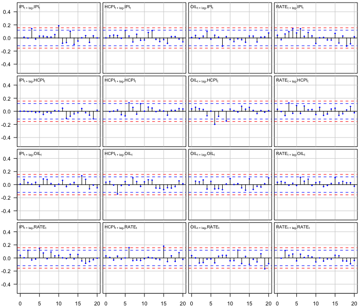
Figure 3: Auto- and crosscorrelation functions of the quantile residuals of the fitted StMVAR($2,2$) model for the lags $0,1,...,20$. The lag zero autocorrelation coefficients are omitted, as they are one by convention. The blue dashed lines are the $95\%$ bounds $\pm 1.96/\sqrt{T}$ ($T=274$ as the first $p=2$ observations were used as the initial values) for autocorrelations of IID observations, whereas the red dashed lines are the corresponding $99\%$ bounds $\pm 2.58/\sqrt{T}$. These bounds are presented to give an approximate perception on the magnitude of the correlation coefficients.

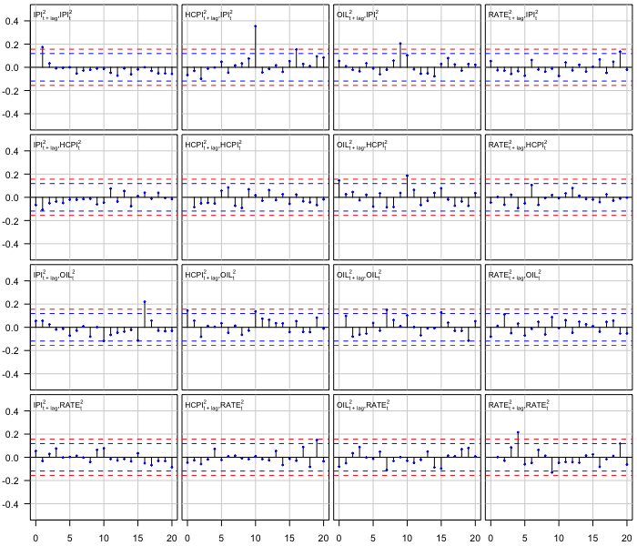
Figure 4: Auto- and crosscorrelation functions of the squared quantile residuals of the fitted StMVAR($2,2$) model for the lags $0,1,...,20$. The lag zero autocorrelation coefficients are omitted, as they are one by convention. The blue dashed lines are the $95\%$ bounds $\pm 1.96/\sqrt{T}$ ($T=274$ as the first $p=2$ observations were used as the initial values) for autocorrelations of IID observations, whereas the red dashed lines are the corresponding $99\%$ bounds $\pm 2.58/\sqrt{T}$. These bounds are presented to give an approximate perception on the magnitude of the correlation coefficients.

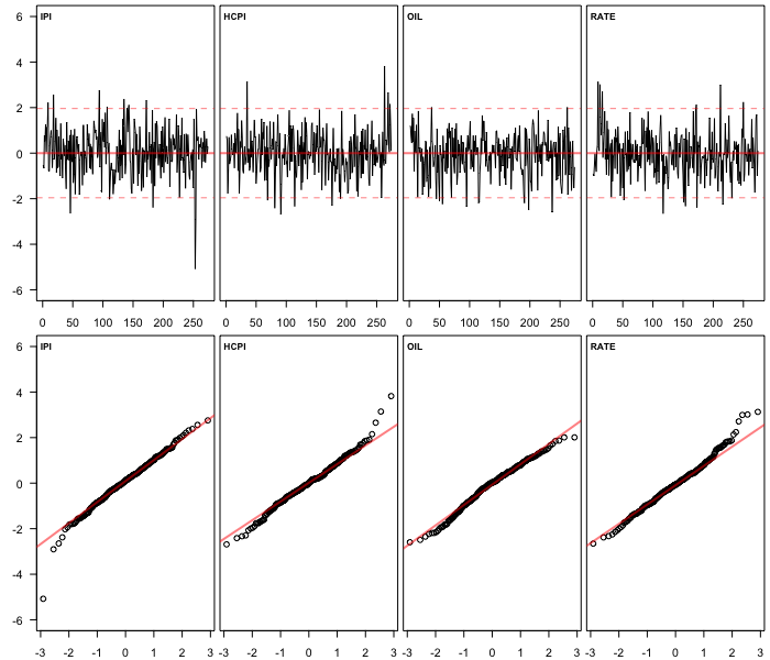
Figure 5: Quantile residual time series and normal quantile-quantile-plots of the fitted StMVAR($2,2$) model.

C.2 Characteristics of the selected model

Table 2 presents the estimates for the mixing weight parameters, degrees of freedom parameters, and the estimated unconditional means and variances of each marginal series (based on the stationary properties of our model). The mixing weight parameters have the interpretation of being the unconditional probabilities for an observation being generated from each regime. For a correctly specified model, they should hence approximately reflect the proportions of observations generated from each regime. The first regime has a mixing weight parameter estimate $0.77$, and it covers approximately $63\%$ of the series (approximated as the mean of the estimated mixing weights), whereas the second regime has the implied mixing weight parameter estimate $0.23$ and it covers approximately $37\%$ of the series. Therefore, they are somewhat disproportionate, but seem reasonable enough not to distort the generalized impulse response functions too much.

			$IPI$		$HCPI$		$OIL$		$RATE$
	$\hat{\alpha}_{m}$	$\hat{\nu}_{m}$	$\hat{\mu}_{m,1}$	$\hat{\sigma}_{m,1}^{2}$	$\hat{\mu}_{m,2}$	$\hat{\sigma}_{m,2}^{2}$	$\hat{\mu}_{m,3}$	$\hat{\sigma}_{m,3}^{2}$	$\hat{\mu}_{m,4}$	$\hat{\sigma}_{m,4}^{2}$
Regime 1	$0.77$	$\phantom{1}3.40$	$-2.89$	$111.22$	$0.12$	$0.08$	$0.02$	$1.79$	$0.24$	$78.96$
Regime 2	$0.23$	$12.89$	$\phantom{-}2.79$	$\phantom{1}10.25$	$0.19$	$0.02$	$0.33$	$0.77$	$2.71$	$\phantom{7}0.47$

Table 2: Mixing weight parameter estimates ($\hat{\alpha}_{m}$), degrees of freedom parameter estimates ($\hat{\nu}_{m}$), and marginal stationary means ($\hat{\mu}_{m,i}$) and variances ($\hat{\sigma}_{m,i}^{2}$) of the component series implied by the fitted StMVAR($2,2$) model for each of the regimes.

The degrees of freedom parameter estimates in Table 2 show that the first regime has fatter tailed distribution than the second one. The first regime also has negative and volatile long-run output gap, while the second regime has positive and less volatile long-run output gap. Long-run inflation, is low in the first regime (roughly $1.4\%$ yearly), whereas it is moderate in the second regime (roughly $2.3\%$ yearly). Also oil price inflation is relatively low in first regime, whereas it is high in the second one. The interest rate variable has low mean in first regime, but the variance is high, which reflects wandering movements of the shadow rate (Wu and Xia, 2016) after the early 2010’s recession. In the second regime, the interest rate variable has moderate mean and low variance. According to the unconditional variances of the observable variables in Table 2, the first regime appears overall more volatile than the second.

According to the estimated mixing weights presented in Figure 1, the first regime (blue) mainly prevails after the collapse of Lehman Brothers in the Financial crisis in September 2008. The first regime also obtains large mixing weights during and before the early 2000’s recession, however. The second regime (red) dominates when the first one does not; that is, mainly before the Financial crisis, but excluding the aforementioned periods when the first regime obtains large mixing weights. After the Financial crisis, the second regime’s mixing weights stay close to zero, excluding a short period before the early 2010’s recession. Because the first regime is characterized by negative output gap and it mainly prevails after the Financial crisis, we refer to it as the low-growth post-Financial crisis regime. Accordingly, because the second regime is characterized by positive output gap and it mainly prevails before the Financial crisis, we refer to it as the high-growth pre-Financial crisis regime.

C.3 Estimates of the structural parameters

The constraints imposed on the B-matrix of the StMVAR($2,2$) model in Section 7.1 produced the following estimates:

$$\hat{W}=\begin{bmatrix}\phantom{-}0.88\ (0.692)&-1.16\ (0.812)&2.00\ (1.164)&-0.40\ (0.351)\\ -0.13\ (0.091)&\phantom{-}0.14\ (0.099)&0.20\ (0.122)&\phantom{-}0\phantom{.00\ (0.000)}\\ -1.20\ (0.686)&-0.42\ (0.561)&0.65\ (0.435)&\phantom{-}0\phantom{.00\ (0.000)}\\ \phantom{-}0.01\ (0.021)&-0.03\ (0.029)&0.06\ (0.045)&\phantom{-}0.56\ (0.313)\\ \end{bmatrix},\ \ \hat{\lambda}_{2}=\begin{bmatrix}0.37\ (0.423)\\ 0.27\ (0.303)\\ 0.14\ (0.161)\\ 0.02\ (0.027)\\ \end{bmatrix},$$ (C.1)

where the identified monetary policy shock is ordered last. The approximate standard errors are presented in parentheses next to the estimates.

References

- Barth and Ramey (2001) Barth M. J., Ramey V. A. (2001). “The Cost Channel of Monetary Transmission.” In BS Bernanke, K Rogoff (eds.), NBER Macroeconomics Annual, volume 16, pp. 199–239. MIT Press, Cambridge.
- Burgard et al. (2019) Burgard J., Neuenkirch M., Nöckel M. (2019). “State-Dependent Transmission of Monetary Policy in the Euro Area.” Journal of Money, Credit and Banking, 51(7), 2053–2070.
- Castelnuovo (2012) Castelnuovo E. (2012). “Testing the Structural Interpretation of the Price Puzzle with a Cost-Channel Model.” Oxford Bulletin of Economics and Statistics, 74(3), 425–452.
- Castelnuovo (2016) Castelnuovo E. (2016). “Monetary policy shocks and Cholesky VARs: an assessment for the Euro area.” Empirical Economics, 50, 383–414.
- Ding (2016) Ding P. (2016). “On the Conditional Distribution of the Multivariate Distribution.” The American Statistician, 70(3), 293–295.
- Dolado and María-Dolores (2006) Dolado J. J., María-Dolores R. (2006). “State Asymmetries in the Effects of Monetary Policy Shocks on Output: Some New Evidence for the Euro-Area.” In C Milas, P Rothman, D van Dijk (eds.), Nonlinear Time Series Analysis of Business Cycles, pp. 311–331. Emerald Publishing Limited.
- Galí (2015) Galí J. (2015). Monetary Policy, Inflation, and the Business Cycle. 2nd edition. Princeton University Press, Princeton and Oxford.
- Gerlach and Lewis (2014) Gerlach S., Lewis J. (2014). “ECB Reaction Functions and the Crisis of 2008.” International Journal of Central Banking, 10(1), 137–158.
- Hamilton (2018) Hamilton J. D. (2018). “WHY YOU SHOULD NEVER USE THE HODRICK-PRESCOTT FILTER.” The Review of Economics and Statistics, 100(5), 831–843.
- Heracleous (2003) Heracleous M. S. (2003). Volatility Modeling Using the Student’s t Distribution. Ph.D. thesis, Virginia Tech.
- Holzmann et al. (2006) Holzmann H., Munk A., Gneiting T. (2006). “Identifiability of finite mixtures of elliptical distributions.” Scandinavian Journal of Statistics, 33(4), 753–763.
- Kalliovirta (2012) Kalliovirta L. (2012). “Misspecification tests based on quantile residuals.” The Econometrics Journal, 15(2), 358–393.
- Kalliovirta et al. (2015) Kalliovirta L., Meitz M., Saikkonen P. (2015). “A Gaussian Mixture Autoregressive Model for Univariate Time Series.” Journal of Time Series Analysis, 36(2), 247–266.
- Kalliovirta et al. (2016) Kalliovirta L., Meitz M., Saikkonen P. (2016). “Gaussian mixture vector autoregression.” Journal of Econometrics, 192(2), 465–498.
- Kalliovirta and Saikkonen (2010) Kalliovirta L., Saikkonen P. (2010). “Reliable Residuals for Multivariate Nonlinear Time Series Models.” Unpublished revision of HECER discussion paper No. 247.
- Kaufmann and Scharler (2009) Kaufmann S., Scharler J. (2009). “Financial systems and the cost channel transmission of monetary policy shocks.” Economic Modelling, 26(1), 40–46.
- Koop et al. (1996) Koop G., Pesaran M., Potter S. (1996). “Impulse response analysis in nonlinear multivariate models.” Journal of Econometrics, 74(1), 119–147.
- Lanne and Lütkepohl (2010) Lanne M., Lütkepohl H. (2010). “Structural Vector Autoregressions With Nonnormal Residuals.” Journal of Business & Economic Statistics, 28(1), 159–168.
- Lanne et al. (2010) Lanne M., Lütkepohl H., Maciejowsla K. (2010). “Structural vector autoregressions with Markov switching.” Journal of Economic Dynamics and Control, 34(2), 121–131.
- Lütkepohl (2005) Lütkepohl H. (2005). New Introduction to Multiple Time Series Analysis. 1st edition. Springer, Berlin.
- Meitz et al. (2018) Meitz M., Preve D., Saikkonen P. (2018). StMAR Toolbox: A MATLAB Toolbox for Student’s t Mixture Autoregressive Models.
- Meitz et al. (forthcoming) Meitz M., Preve D., Saikkonen P. (forthcoming). “A mixture autoregressive model based on Student’s -distribution.” Communications in Statistics - Theory and Methods.
- Meitz and Saikkonen (2021) Meitz M., Saikkonen P. (2021). “Testing for observation-dependent regime switching in mixture autoregressive models.” Journal of Econometrics, 222(1), 601–624.
- Meyn and Tweedie (2009) Meyn S., Tweedie R. (2009). Markov Chains and Stochastic Stability. 2nd edition. Cambridge University Press, Cambridge.
- Muirhead (1982) Muirhead R. (1982). Aspects of Multivariate Statistical Theory. 1st edition. John Wiley & Sons, Hoboken, New Jersey.
- Newey and McFadden (1994) Newey W., McFadden D. (1994). “Large sample estimation and hyphothesis testing.” In R Eagle, D MacFadden (eds.), Handbook of Econometrics, volume 4, chapter 36. Elsevier Science B.V.
- Peersman and Smets (2002) Peersman G., Smets F. (2002). “Are the effects of monetary policy in the euro area greater in recessions than in booms?” In L Mahadeva, P Sinclair (eds.), Monetary Transmission in Diverse Economies, pp. 28–48. Cambridge University Press.
- Pellegrino (2018) Pellegrino G. (2018). “Uncertainty and the real effects of monetary policy shocks in the Euro area.” Economics Letters, 162, 177–181.
- Poudyal (2012) Poudyal N. (2012). Confronting Theory with Data: the Case of DSGE Modeling. Ph.D. thesis, Virginia Tech.
- Rabanal (2007) Rabanal P. (2007). “Does inflation increase after a monetary policy tightening? Answers based on an estimated DSGE model.” Journal of Economic Dynamics and Control, 31(3), 906–937.
- Ranga Rao (1962) Ranga Rao R. (1962). “Relations between Weak and Uniform Convergence of Measures with Applications.” The Annals of Mathematical Statistics, 33(2), 659–680.
- Ravenna and Walsh (2006) Ravenna F., Walsh C. (2006). “Optimal monetary policy with the cost channel.” Journal of Monetary Economics, 53(2), 199–216.
- Redner and Walker (1984) Redner R., Walker H. (1984). “Mixture Densities, Maximum Likelihood and the Em Algorithm.” Society for Industrial and Applied Mathematics, 26(2), 195–239.
- Sims (1992) Sims A. (1992). “Interpreting the macroeconomic time series facts.” European economic review, 36(5), 975–1000.
- Virolainen (2018a) Virolainen S. (2018a). gmvarkit: Estimate Gaussian and Student’s Mixture Vector Autoregressive Models. R package version 2.0.3 available at CRAN: https://CRAN.R-project.org/package=gmvarkit.
- Virolainen (2018b) Virolainen S. (2018b). uGMAR: Estimate Univariate Gaussian and Student’s Mixture Autoregressive Models. R package version 3.4.2 available at CRAN: https://CRAN.R-project.org/package=uGMAR.
- Virolainen (2022) Virolainen S. (2022). “Structural Gaussian Mixture vector autoregressive model with application to the asymmetric effects of monetary policy shocks.” Unpublished working paper, available as arXiv:2007.04713.
- Virolainen (forthcoming) Virolainen S. (forthcoming). “A mixture autoregressive model based on Gaussian and Student’s -distributions.” Studies in Nonlinear Dynamics & Econometrics.
- Wu and Xia (2016) Wu J., Xia F. (2016). “Measuring the Macroeconomic Impact of Monetary Policy at the Zero Lower Bound.” Journal of Money, Credit and Banking, 48(2-3), 253–291.