On eigenvalues of a high-dimensional Kendall’s rank correlation matrix with dependence

Abstract

This paper investigates limiting spectral distribution of a high-dimensional Kendall’s rank correlation matrix. The underlying population is allowed to have general dependence structure. The result no longer follows the generalized Marc̆enko-Pastur law, which is brand new. It’s the first result on rank correlation matrices with dependence. As applications, we study the Kendall’s rank correlation matrix for multivariate normal distributions with a general covariance matrix. From these results, we further gain insights on Kendall’s rank correlation matrix and its connections with the sample covariance/correlation matrix.

, , and

1 Introduction

Covariance and correlation matrices play a vital role in multivariate statistical analysis because they provide the most direct way to characterize the relation between different variables. Many statistical estimation or inference methods involve the covariance or correlation matrix, such as principal component analysis, multivariate analysis of variance, factor analysis, etc. In high-dimensional data analysis, studying the eigenvalues and eigenvectors of such covariance/correlation matrices are fundamental problems.

In random matrix theory, sample covariance matrix has been thoroughly studied in the past decades. For an $n\times n$ Hermitian matrix $\mathbf{H}_{n}$, the Empirical Spectral Distribution (ESD) of $\mathbf{H}_{n}$ is defined as

$$F^{\mathbf{H}_{n}}(x)=\frac{1}{n}\sum_{i=1}^{n}I(\lambda_{i}\leq x),$$

where $\lambda_{1},\cdots,\lambda_{n}$ are eigenvalues of $\mathbf{H}_{n}$ and $I(\cdot)$ is the indicator function. If $F^{\mathbf{H}_{n}}$ converges to a deterministic distribution function $F$, then $F(x)$ is called the Limiting Spectral Distribution (LSD) of $\mathbf{H}_{n}$. Marc̆enko and Pastur (1967) first derived the LSD of the sample covariance matrix. Further, Bai and Silverstein (2004) studied the Central Limit Theorem (CLT) for its Linear Spectral Statistics (LSSs) defined as

$$\frac{1}{n}\sum_{i=1}^{n}f(\lambda_{i})=\int f(x)dF^{\mathbf{H}_{n}}(x),$$

where $f(\cdot)$ is a function on $\mathbb{R}^{+}$. As we know, many important statistics in multivariate analysis can be expressed through ESD, for example,

$$\frac{1}{n}\mbox{tr}(\mathbf{H}_{n})=\frac{1}{n}\sum_{i=1}^{n}\lambda_{i}=\int xdF^{\mathbf{H}_{n}}(x)$$

and

$$\frac{1}{n}\log|\mathbf{H}_{n}|=\frac{1}{n}\sum_{i=1}^{n}\log{(\lambda_{i})}=\int\log{(x)}dF^{\mathbf{H}_{n}}(x).$$

Generally, LSD describes the first-order limits of these LSSs and CLT then characterizes their second-order asymptotics. The two are the analogs of Law of Large Numbers and Central Limit Theorem in classical probability theory, respectively. As applications, CLT for LSSs provides an important tool for many hypothesis testing problems in multivariate analysis with diverging data dimension, e.g., Bai et al. (2009) derived the distribution of the likelihood ratio test for high-dimensional data. Both LSD and CLT for LSSs study the global law of the empirical eigenvalues. Another fundamental problem is the local law (Knowles and Yin, 2017), e.g., the asymptotic behaviors of the smallest and largest eigenvalues. The well-known Bai-Yin law (Bai and Yin, 1993) derived the limits of the extreme eigenvalues. Johnstone (2001) further established the Tracy-Widom law for the largest eigenvalues, which plays a fundamental role in principal component analysis. For more comprehensive overview on this topic, one is referred to Bai and Silverstein (2010).

In practice, data normalization is a standard procedure and after that, we are actually dealing with the sample correlation matrix (El Karoui, 2009). Parallel to the study of the sample covariance matrix, Jiang (2004) first obtained the LSD of Pearson-type sample correlation matrix and Gao et al. (2017) developed the CLT for its LSSs. Bao, Pan and Zhou (2012) established the Tracy-Widom law for its extreme eigenvalues and Pillai and Yin (2012) extended the result to general cases. However, due to the complex structure of the sample correlation matrix, most results only consider the case that sample data has independent components so that its population covariance matrix is diagonal and then the correlation matrix is identity. From the perspective of applications, the independence assumption is however too strong so that such results have very limited applicability (El Karoui, 2009). On the other hand, for general dependent or correlated data, little work (e.g., El Karoui, 2009; Morales-Jimenez et al., 2021) has been done on the sample correlation matrix. As far as the CLT for LSSs, the existing works include Mestre and Vallet (2017) that considered the case for Gaussian distributions and Zheng et al. (2019) studied the trace moments.

For the sample covariance/correlation matrix, due to the congenital sensitivity of Pearson-type correlation, finite fourth order or even higher order moments of the data distribution are usually required to guarantee the convergence of the limiting distributions. However, most of the results applicable to light-tailed distributions cannot be directly extended to heavy-tailed cases, e.g., Heiny and Yao (2020) explored the spectral behavior of Pearson-type correlations for heavy-tail distributions where the story becomes completely different.

As a remedy for dealing with heavy-tailed data samples, some non-parametric correlation matrix, such as Kendall’s $\tau$ and Spearman’s $\rho$, have received considerable attention in recent years. Kendall’s $\tau$ and Spearman’s $\rho$ are rank-based and thus there’s no need to impose any moment restrictions on the underlying distribution. What is more, classical theory on non-parametric statistics shows that only partial information will be lost while robustness can be retained if we only use the ranks of the data. In random matrix theory, Bai and Zhou (2008) first derived the LSD of Spearman’s rank correlation matrix, which turns out to be the same as the standard Marc̆enko-Pastur law. For the Kendall’s $\tau$, Bandeira, Lodhia and Rigollet (2017) proved that its LSD is an affine transformation of the standard Marc̆enko-Pastur law. For the CLT for LSSs, Bao et al. (2015) considered Spearman’s rank correlation matrix and Li, Wang and Li (2021) studied Kendall’s rank correlation matrix. The Tracy-Widom law for the extreme eigenvalues of the two matrices can be found in Bao (2019a) and Bao (2019b), respectively. However, all these asymptotic results are for data sample with independent components, i.e., all components are independent. To the best of our knowledge, there are no available results on such rank correlation matrices when the underlying distribution has general dependent structure. We summarize the developments of the sample covariance matrix, sample correlation matrix, Kendall’s $\tau$ and Spearman’s $\rho$ in Table 1.1.

Table 1.1: Developments of sample covariance/correlation matrices in random matrix theory

	Sample covariance	Sample correlation	Kendall’s $\tau$	Spearman’s $\rho$
	Independent case ($\mbox{\boldmath$\Sigma$}=\mathbf{I}$)
LSD	Marc̆enko and Pastur (1967)	Jiang (2004)	Bandeira, Lodhia and Rigollet (2017)	Bai and Zhou (2008)
CLT for LSSs	Bai and Silverstein (2004)	Gao et al. (2017)	Li, Wang and Li (2021)	Bao et al. (2015)
Tracy-Widom	Johnstone (2001)	Bao, Pan and Zhou (2012)	Bao (2019b)	Bao (2019a)
	Dependent case (general $\Sigma$)
LSD	Marc̆enko and Pastur (1967)	El Karoui (2009)
CLT for LSSs	Bai and Silverstein (2004)	Mestre and Vallet (2017)
Tracy-Widom	Féral and Péché (2009)

As can be seen from Table 1.1, the asymptotic behaviors of the eigenvalues of the rank correlation matrices under general dependent structure is still unclear. In this paper, we take the first step to fill this gap and focus on Kendall’s rank correlation matrix with high-dimensional correlated data. Specifically, for data sample $\mathbf{x}_{1},\cdots,\mathbf{x}_{n}\in\mathbb{R}^{p}$, we define the sign vector

$$\mathbf{A}_{ij}=\mbox{sign}(\mathbf{x}_{i}-\mathbf{x}_{j})=\left(\mbox{sign}(x_{i1}-x_{j1}),\cdots,\mbox{sign}(x_{ip}-x_{jp})\right)^{\mathrm{\scriptscriptstyle T}}$$

where $\mbox{sign}(\cdot)$ denotes the sign function and the sample Kendall’s rank correlation matrix (Kendall, 1938)

$$\mathbf{K}_{n}=\frac{2}{n(n-1)}\sum_{1\leq i<j\leq n}\mathbf{A}_{ij}\mathbf{A}^{\mathrm{\scriptscriptstyle T}}_{ij}.$$ (1.1)

Our goal is to study the spectral properties of $\mathbf{K}_{n}$ when $\mathbf{x}_{i}^{\prime}s$ have a general dependent structure. This is a problem of its own significant interest in random matrix theory. To study Kendall’s rank correlation matrix with dependence, LSD is the cornerstone for further derivations of CLT for LSSs (Bai and Silverstein, 2004) and local laws including the asymptotic distribution of extreme eigenvalues (Knowles and Yin, 2017). It’s also a key step to solve many high-dimensional statistical problems with heavy-tailed observations. Taking high-dimensional independent test as an example, many test statistics based on covariance/correlation matrices have been proposed to test complete independence among the components of $\mathbf{x}_{i}^{\prime}s$; see Schott (2005), Bao et al. (2015), Gao et al. (2017), Leung and Drton (2018), Bao (2019b), Li, Wang and Li (2021) etc. In particular, Leung and Drton (2018) and Li, Wang and Li (2021) considered test statistics that based on linear functions of the eigenvalues of Kendall’s $\tau$, e.g., $\mbox{tr}(\mathbf{K}_{n}^{2})$ and $\log|\mathbf{K}_{n}|$. However, the test power is still unclear since the limiting properties of Kendall’s $\tau$ (also Spearman’s $\rho$) under general dependent alternatives remain largely unknown.

To answer such questions, in this paper, we take the first step to derive the limiting spectral distribution of $\mathbf{K}_{n}$ under the asymptotic regime where $p,n\rightarrow\infty$ and $p/n\rightarrow c\in(0,\infty)$. One major challenge is the nonlinear dependent structure among the sign-based summands $\mathbf{A}_{ij}$ of $\mathbf{K}_{n}$. Hence, we apply the Hoeffding decomposition to $\mathbf{A}_{ij}$ to locate the leading terms. In this way, we obtain the equation which the Stieltjes transform of the limiting spectral distribution of $\mathbf{K}_{n}$ satisfies. It’s a brand new distribution which relies heavily on both the covariance and conditional covariance structure of $\mathbf{A}_{ij}$. As illustration, we study the normal distribution where the Kendall’s rank correlation has a specific relation with the Pearson’s correlation and then we derive explicit LSDs for some cases with common dependent structure. Simulation experiments also lend full support to the accuracy of our theoretical results.

The rest of the paper is organized as follows. Section 2 introduces some preliminary knowledge on Kendall’s rank correlation matrix and Hoeffding decomposition. Section 3 contains our main results on the LSD of Kendall’s rank correlation matrix for correlated data. Section 4 considers the Gaussian distributions and Section 5 collects all the numerical experiments. Proofs of the main results are given in the Appendix.

2 Background on Kendall’s rank correlation matrix

2.1 Kendall’s rank correlation matrix

From the definition of Kendall’s rank correlation matrix (1.1), we can write

$$\mathbf{K}_{n}=\frac{2}{n(n-1)}\sum_{1\leq i<j\leq n}\mbox{sign}\left(\frac{\mathbf{x}_{i}-\mathbf{x}_{j}}{\sqrt{2}}\right)\mbox{sign}\left(\frac{\mathbf{x}_{i}-\mathbf{x}_{j}}{\sqrt{2}}\right)^{\mathrm{\scriptscriptstyle T}},$$

which looks similar with the sample covariance matrix. To be specific, the sample covariance matrix of the data sample $\mathbf{x}_{1},\cdots,\mathbf{x}_{n}\in\mathbb{R}^{p}$ can be written as an U-statistic of order two, i.e.,

$$\mathbf{S}_{n}=\frac{1}{n-1}\sum_{i=1}^{n}(\mathbf{x}_{i}-\bar{\mathbf{x}})(\mathbf{x}_{i}-\bar{\mathbf{x}})^{\mathrm{\scriptscriptstyle T}}=\frac{2}{n(n-1)}\sum_{1\leq i<j\leq n}\left(\frac{\mathbf{x}_{i}-\mathbf{x}_{j}}{\sqrt{2}}\right)\left(\frac{\mathbf{x}_{i}-\mathbf{x}_{j}}{\sqrt{2}}\right)^{\mathrm{\scriptscriptstyle T}}.$$ (2.1)

Despite this similarity in their forms, the inner structure of the two matrices does not follow the same pattern. The sign function introduces non-linear correlation into the matrix $\mathbf{K}_{n}$ and it is nontrivial to analyze such correlation even for binary random variables. For example, Esscher (1924) spent a lot of efforts to derive the variance of Kendall’s rank correlation for bi-normal distributions. As can be seen from Childs (1967), it is already quite complicated to calculate the integral of sign function over fourth order even for normal distribution. Thus, for high-dimensional Kendall’s rank correlation matrix, it is very challenging to study its asymptotic properties.

One appealing property of Kendall’s rank correlation is that it is monotonically invariant (Weihs, Drton and Meinshausen, 2018).

Proposition 2.1 (Monotonic Invariance).

For any strictly increasing monotonic functions $f_{j}(\cdot),j=1,\ldots,p$, $\mathbf{K}_{n}$ is invariant for monotonic component transformation

$$\mathbf{x}_{i}=(x_{i1},\cdots,x_{ip})^{\mathrm{\scriptscriptstyle T}}\mapsto\big{(}f_{1}(x_{i1}),\cdots,f_{p}(x_{ip})\big{)}^{\mathrm{\scriptscriptstyle T}}.$$

The reason is that Kendall’s rank correlation is rank-based and the monotonic transformation does not change the order statistics. One special case is that for any linear transformation of the data

$$\mathbf{x}_{i}=(x_{i1},\cdots,x_{ip})^{\mathrm{\scriptscriptstyle T}}\mapsto(\mu_{1}+\sigma_{1}x_{i1},\cdots,\mu_{p}+\sigma_{p}x_{i1})^{\mathrm{\scriptscriptstyle T}},$$

their corresponding Kendall’s rank correlations remain unchanged. That is, Kendall’s $\tau$ is a correlation matrix which is invariant to the location and scale. More importantly, for any distribution, Kendall’s rank correlation always exists and this fact makes it an important tool to characterize data with heavy tails.

In previous works on Kendall’s rank correlation matrix for high-dimensional data (e.g., Bandeira, Lodhia and Rigollet 2017, Leung and Drton 2018, Bao 2019b, Li, Wang and Li 2021), they assumed that all the components were independent with absolutely continuous density. By the monotonic invariance, we can always transform each component into a standard normal distribution and all components are still independent. Thus, it can be formulated as that $\mathbf{x}_{1},\ldots,\mathbf{x}_{n}$ are independent and identically distributed (i.i.d.) from a standard multivariate normal distribution $N(0,\mathbf{I}_{p})$, from which we can see that these results are very limited. In this work, we consider more general cases where the data components are allowed to have dependence.

2.2 Hoeffding decomposition

In this part, to deal with the nonlinear dependent structure of high-dimensional Kendall’s rank correlation matrix, we apply Hoeffding decomposition to find out the leading terms. Specifically, denote $\mathbf{A}_{i}$ as the conditional expectation of $\mathbf{A}_{ij}$ given $\mathbf{x}_{i}$,

$$\mathbf{A}_{i}\stackrel{{\scriptstyle\mbox{{\tiny def}}}}{{=}}\mathbb{E}\{\mbox{sign}(\mathbf{x}_{i}-\mathbf{x})\mid\mathbf{x}_{i}\},$$ (2.2)

the Hoeffding decomposition for $\mathbf{A}_{ij}$ can be written as,

$$\mathbf{A}_{ij}=\mathbf{A}_{i}-\mathbf{A}_{j}+\epsilon_{ij},$$ (2.3)

where

$$\epsilon_{ij}=\mbox{sign}(\mathbf{x}_{i}-\mathbf{x}_{j})-\mathbb{E}\{\mbox{sign}(\mathbf{x}_{i}-\mathbf{x}_{j})\mid\mathbf{x}_{i}\}+\mathbb{E}\{\mbox{sign}(\mathbf{x}_{i}-\mathbf{x}_{j})\mid\mathbf{x}_{j}\}.$$

Throughout this paper, we assume that $\mathbf{x}_{1},\ldots,\mathbf{x}_{n}$ are i.i.d. from a population with absolutely continuous density. Then, we have

$$\mathbb{E}(\mathbf{A}_{ij})=\mathbb{E}(\mathbf{A}_{i})=\mathbb{E}(\epsilon_{ij})=\mathbf{0},$$

and the covariance matrices of $\mathbf{A}_{ij},~{}\mathbf{A}_{i}$ and $\epsilon_{ij}$ exist. Specially, we denote

$$\mbox{\boldmath$\Sigma$}_{1}\stackrel{{\scriptstyle\mbox{{\tiny def}}}}{{=}}\mbox{cov}(\mathbf{A}_{ij}),\quad\mbox{\boldmath$\Sigma$}_{2}\stackrel{{\scriptstyle\mbox{{\tiny def}}}}{{=}}\mbox{cov}(\mathbf{A}_{i}),\quad\mbox{cov}(\epsilon_{ij})=\mbox{\boldmath$\Sigma$}_{1}-2\mbox{\boldmath$\Sigma$}_{2}\stackrel{{\scriptstyle\mbox{{\tiny def}}}}{{=}}\mbox{\boldmath$\Sigma$}_{3}.$$ (2.4)

2.3 Preliminary results

With the Hoeffding decomposition of $\mathbf{A}_{ij}$ described in (2.3), the Kendall’s rank correlation matrix $\mathbf{K}_{n}$ can be decomposed accordingly,

$$\mathbf{K}_{n} =\frac{2}{n(n-1)}\sum_{1\leq i<j\leq n}(\mathbf{A}_{i}-\mathbf{A}_{j}+\epsilon_{ij})(\mathbf{A}_{i}-\mathbf{A}_{j}+\epsilon_{ij})^{\mathrm{\scriptscriptstyle T}}$$

$$=\frac{2}{n(n-1)}\sum_{1\leq i<j\leq n}(\mathbf{A}_{i}-\mathbf{A}_{j})(\mathbf{A}_{i}-\mathbf{A}_{j})^{\mathrm{\scriptscriptstyle T}}+\frac{2}{n(n-1)}\sum_{1\leq i<j\leq n}(\mathbf{A}_{i}-\mathbf{A}_{j})\epsilon_{ij}^{\mathrm{\scriptscriptstyle T}}$$

$$\quad+\frac{2}{n(n-1)}\sum_{1\leq i<j\leq n}\epsilon_{ij}(\mathbf{A}_{i}-\mathbf{A}_{j})^{\mathrm{\scriptscriptstyle T}}+\frac{2}{n(n-1)}\sum_{1\leq i<j\leq n}\epsilon_{ij}\epsilon_{ij}^{\mathrm{\scriptscriptstyle T}}$$

$$=\mathbf{M}_{1}+\mathbf{M}_{2}+\mathbf{M}_{2}^{\mathrm{\scriptscriptstyle T}}+\mathbf{M}_{3},$$ (2.5)

where

$$\mathbf{M}_{1}\stackrel{{\scriptstyle\mbox{{\tiny def}}}}{{=}}\frac{2}{n(n-1)}\sum_{1\leq i<j\leq n}(\mathbf{A}_{i}-\mathbf{A}_{j})(\mathbf{A}_{i}-\mathbf{A}_{j})^{\mathrm{\scriptscriptstyle T}}=\frac{2}{n-1}\sum_{i=1}^{n}(\mathbf{A}_{i}-\bar{\mathbf{A}})(\mathbf{A}_{i}-\bar{\mathbf{A}})^{\mathrm{\scriptscriptstyle T}},$$

$$\mathbf{M}_{2}\stackrel{{\scriptstyle\mbox{{\tiny def}}}}{{=}}\frac{2}{n(n-1)}\sum_{1\leq i<j\leq n}(\mathbf{A}_{i}-\mathbf{A}_{j})\epsilon_{ij}^{\mathrm{\scriptscriptstyle T}},\quad\mathbf{M}_{3}\stackrel{{\scriptstyle\mbox{{\tiny def}}}}{{=}}\frac{2}{n(n-1)}\sum_{1\leq i<j\leq n}\epsilon_{ij}\epsilon_{ij}^{\mathrm{\scriptscriptstyle T}},$$

and $\bar{\mathbf{A}}=\frac{1}{n}\sum_{i=1}^{n}\mathbf{A}_{i}$. In particular, $\mathbf{M}_{1}$ is the sample covariance matrix formed by i.i.d. random vectors $\mathbf{A}_{1},\ldots,\mathbf{A}_{n}$, see the illustration in (2.1).

Our first result is to show that the error terms $\mathbf{M}_{2}$ and $\mathbf{M}_{3}-\mathbb{E}(\mathbf{M}_{3})$ can be controlled so that the dominant contribution in terms of the LSD of $\mathbf{K}_{n}$ is from $\mathbf{M}_{1}$. As a result, we define the following matrix

$$\mathbf{W}_{n}\stackrel{{\scriptstyle\mbox{{\tiny def}}}}{{=}}\mathbf{M}_{1}+\mbox{\boldmath$\Sigma$}_{3}=\frac{2}{n-1}\sum_{i=1}^{n}(\mathbf{A}_{i}-\bar{\mathbf{A}})(\mathbf{A}_{i}-\bar{\mathbf{A}})^{\mathrm{\scriptscriptstyle T}}+\mbox{\boldmath$\Sigma$}_{3}.$$ (2.6)

Throughout the paper, we use $\|\cdot\|$ and $\|\cdot\|_{2}$ to denote the common spectral norm and Frobenius norm of a matrix, respectively.

Proposition 2.2.

Assume $\|\mbox{\boldmath$\Sigma$}_{1}\|\leq C$ for some universal constant $C$ and

$$\frac{1}{p^{2}}\mbox{var}\left(\mathbf{A}_{12}^{\mathrm{\scriptscriptstyle T}}\mathbf{A}_{13}\right)\to 0,$$

then we have

$$L(F^{\mathbf{K}_{n}},F^{\mathbf{W}_{n}})\to 0,~{}\mbox{in~{}probability}$$

where $L(\cdot,\cdot)$ is the Levy distance between two distributions.

Remark 2.3.

The assumptions on $\|\mbox{\boldmath$\Sigma$}_{1}\|$ and $\mbox{var}\left(\mathbf{A}_{12}^{\mathrm{\scriptscriptstyle T}}\mathbf{A}_{13}\right)$ are to avoid too strong dependence among the components of the data. In random matrix theory, it is a regular condition to assume that the norm of the population covariance matrix is uniformly bounded, e.g., Condition 3 in Bai and Zhou (2008). Here, this condition is also required for bounding the difference between $\mathbf{K}_{n}$ and $\mathbf{W}_{n}$. To show that such condition $\|\mbox{\boldmath$\Sigma$}_{1}\|\leq C$ is necessary, we conduct a toy example in the following. Specifically, we generate $n$ data sample $\mathbf{x}_{1},\ldots,\mathbf{x}_{n},i.i.d\sim N(0,\mbox{\boldmath$\Sigma$})$ where $\Sigma$ is a matrix with $\Sigma_{ii}=1$ and $\Sigma_{ij}=\rho$. For this case,

$$\|\mbox{\boldmath$\Sigma$}_{1}\|=1+\frac{2}{\pi}(p-1)\arcsin(\rho),$$

which is unbounded for any $\rho>0$. Figure 1 presents the distance $\|\mathbf{K}_{n}-\mathbf{W}_{n}\|_{2}^{2}/p$ versus the increasing $\rho$, and from which we can see that $\|\mbox{\boldmath$\Sigma$}_{1}\|\leq C$ is necessary for bounding the difference between $F^{\mathbf{K}_{n}}$ and $F^{\mathbf{W}_{n}}$.

Figure 1: Plots of the scaled squared Frobenius norm of $\mathbf{K}_{n}-\mathbf{W}_{n}$ versus $\rho\in[0,0.9]$. Data sample $\mathbf{x}_{1},\cdots,\mathbf{x}_{n}$ are generated from a multivariate normal distribution $N_{p}(0,\mbox{\boldmath$\Sigma$})$ with $\Sigma_{ii}=1$ and $\Sigma_{ij}=\rho$. Here $(n,p)=(100,200)$ and the results are based on 100 replications.

Noting that $\mathbf{A}_{1},\ldots,\mathbf{A}_{n}$ are i.i.d. random vectors with covariance matrix $\mbox{cov}(\mathbf{A}_{i})=\mbox{\boldmath$\Sigma$}_{2}$ and

$$\mathbb{E}\mathbf{K}_{n}=\mbox{\boldmath$\Sigma$}_{1}=2\mbox{\boldmath$\Sigma$}_{2}+\mbox{\boldmath$\Sigma$}_{3}.$$

Proposition 2.2 shows that part of Kendall’s rank correlation matrix has similar fluctuations as the usual sample covariance matrix with population covariance matrix $2\mbox{\boldmath$\Sigma$}_{2}$ and the other part is concentrated on the deterministic matrix $\mbox{\boldmath$\Sigma$}_{3}$. This phenomenon is an analogy of Hoeffding decomposition for the classical U-statistics. By implementing the Hoeffding decomposition for the random vector $\mathbf{A}_{ij}$, we then transfer the study of the LSD of $\mathbf{K}_{n}$ to the study of the LSD of $\mathbf{W}_{n}$.

3 Limiting spectral distribution of $\mathbf{K}_{n}$

In this section, we present the LSD of the Kendall’s rank correlation matrix $\mathbf{K}_{n}$. We first introduce the concept of Stieltjes transform, which is an important tool in random matrix theory. Letting $\mu$ be a finite measure on $\mathbb{R}$, its Stieltjes transform $s_{\mu}(z)$ is defined as

$$s_{\mu}(z)=\int\frac{1}{x-z}\mu(dx),~{}z\in\mathbb{C}^{+},$$

where $\mathbb{C}^{+}$ denotes the upper complex plane. We can also obtain $\mu$ from $s_{\mu}(z)$ by the inversion formula. For any two continuity points $a<b$ of $\mu$, we have

$$\mu([a,b])=\lim_{\nu\to 0^{+}}\frac{1}{\pi}\int_{a}^{b}\Im s_{\mu}(x+i\nu)dx,$$ (3.1)

where $\Im$ is the imaginary part of a complex number and $i$ is the imaginary unit.

For Kendall’s rank correlation matrix, Bandeira, Lodhia and Rigollet (2017) derived the LSD when the observations $\mathbf{x}_{1},\ldots,\mathbf{x}_{n}$ are i.i.d. random vectors and the components are also independent with absolutely continuous density. They show that as $n\rightarrow\infty$, $p/n\rightarrow c\in(0,\infty)$, the ESD of such Kendall’s rank converges in probability to an affine transformation of the standard Mar$\check{\mbox{c}}$enko-Pastur law with parameter $c$, which has an explicit form whose density function $p_{c}(x)$ is given by

$$p_{c}(x)=\frac{9}{4\pi c(3x-1)}\sqrt{(c_{+}-x)(x-c_{-})}+(1-1/c)\delta_{\frac{1}{3}}I(c>1),~{}c_{-}\leq x\leq c_{+},$$

where $c_{-}=\frac{1}{3}+\frac{2}{3}(1-\sqrt{c})^{2}$ and $c_{+}=\frac{1}{3}+\frac{2}{3}(1+\sqrt{c})^{2}$. The corresponding Stieltjes transform $s(z)\in\mathbb{C}^{+}$ is the unique solution to the following equation

$$\frac{2}{3}c\left(z-\frac{1}{3}\right)s^{2}(z)+\left(z-1+\frac{2}{3}c\right)s(z)+1=0.$$ (3.2)

To illustrate the challenges of Kendall’s rank correlation matrix in random matrix theory, we consider the ranking of the data

$$\begin{pmatrix}\mathbf{x}_{1}^{\mathrm{\scriptscriptstyle T}}\\ \vdots\\ \mathbf{x}_{n}^{\mathrm{\scriptscriptstyle T}}\end{pmatrix}=\underbrace{\begin{pmatrix}x_{11}&\cdots&x_{1p}\\ \vdots&\vdots&\vdots\\ x_{n1}&\cdots&x_{np}\\ \end{pmatrix}}_{\text{raw data matrix}}\Longrightarrow\underbrace{\ \begin{pmatrix}r_{11}&\cdots&r_{1p}\\ \vdots&\vdots&\vdots\\ r_{n1}&\cdots&r_{np}\\ \end{pmatrix}}_{\text{ranking matrix}},$$

where each column $(r_{1j},\ldots,r_{nj})$ are the rank of the raw data $(x_{1j},\ldots,x_{nj})$. For i.i.d. sample $\mathbf{x}_{1},\cdots,\mathbf{x}_{n}\in\mathbb{R}^{p}$, each column of the ranking matrix follows the uniform distribution on the set of all $n!$ permutations of $\{1,2,\cdots,n\}$. While the rows of the raw data matrix are independent, the ranking matrix dose not have independent rows anymore. For the special case where the columns of the raw data are also independent (e.g., Bandeira, Lodhia and Rigollet 2017, Leung and Drton 2018, Bao 2019b, Li, Wang and Li 2021), the columns of the ranking matrix will be independent. Then, the raw data is actually with i.i.d entries which has very limited applications. If the columns of the raw data are dependent, e.g., there is a covariance structure among components, both the rows and the columns of the ranking matrix are dependent. From the perspective of random matrix theory, analyzing such matrices is very challenging.

We first provide a general result as follows and then study the case for Gaussian distribution in the next section.

Theorem 3.1.

For i.i.d. continuous data sample $\mathbf{x}_{1},\cdots,\mathbf{x}_{n}\in\mathbb{R}^{p}$, assume that

• as $p\to\infty$,

  $$\frac{1}{p^{2}}\mbox{var}\left(\mathbf{A}_{12}^{\mathrm{\scriptscriptstyle T}}\mathbf{A}_{13}\right)\to 0,\text{and}~{}~{}\frac{1}{p^{2}}\mbox{var}(\mathbf{A}_{1}^{\mathrm{\scriptscriptstyle T}}\mathbf{B}\mathbf{A}_{1})\to 0,$$ (3.3)

  where $\mathbf{B}$ is any deterministic matrix with bounded spectral norm;

• $\|\mbox{\boldmath$\Sigma$}_{1}\|\leq C$ for some universal constant $C$, also the solution $x(z)\in\mathbb{C}^{-}$ to the following equation exists

  $$\frac{1}{x(z)}=1+\lim_{n\to\infty}\frac{2}{n}\mbox{tr}\big{[}(\mbox{\boldmath$\Sigma$}_{3}+2x(z)\mbox{\boldmath$\Sigma$}_{2}-z\mathbf{I}_{p})^{-1}\mbox{\boldmath$\Sigma$}_{2}\big{]};$$ (3.4)

• $p,n\rightarrow\infty$ such that $p/n\rightarrow c\in(0,\infty)$.

Then, in probability, the empirical spectral distribution $F^{\mathbf{K}_{n}}$ converges weakly to a limiting spectral distribution $F$ whose Stieltjes transform $s(z)$ is given by

$$s(z)=\lim_{p\to\infty}\frac{1}{p}\mbox{tr}\big{[}(\mbox{\boldmath$\Sigma$}_{3}+2x(z)\mbox{\boldmath$\Sigma$}_{2}-z\mathbf{I}_{p})^{-1}\big{]}.$$ (3.5)

Recall the dominating matrix $\mathbf{W}_{n}$ in (2.6), which has the same LSD as the following matrix

$$\frac{2}{n}\sum_{i=1}^{n}\mathbf{A}_{i}\mathbf{A}^{\mathrm{\scriptscriptstyle T}}_{i}+\mbox{\boldmath$\Sigma$}_{3}.$$ (3.6)

The first part $n^{-1}\sum_{i=1}^{n}\mathbf{A}_{i}\mathbf{A}^{\mathrm{\scriptscriptstyle T}}_{i}$ is the type of a sample covariance matrix corresponding to the data sample $\{\mathbf{A}_{i}\}$ with population covariance matrix $\mbox{cov}(\mathbf{A}_{i})=\mbox{\boldmath$\Sigma$}_{2}$. However, the components within $\mathbf{A}_{i}$ are nonlinearly correlated and thus can not be written in the form of independent components model such that $\mathbf{A}_{i}=\mbox{\boldmath$\Sigma$}^{1/2}_{2}\mathbf{z}_{i}$. For those weakly dependent data sample, Bai and Zhou (2008) proved that under certain conditions, the LSD of the sample covariance matrix still follows the generalized Marc̆enko-Pastur law. One of the crucial conditions is that the variance of the quadratic forms $\mathbf{A}_{i}^{\mathrm{\scriptscriptstyle T}}\mathbf{B}\mathbf{A}_{i}$ is relatively small (see Theorem 1.1 in Bai and Zhou 2008), i.e.,

$$\mbox{var}(\mathbf{A}_{i}^{\mathrm{\scriptscriptstyle T}}\mathbf{B}\mathbf{A}_{i})=o(n^{2}),$$

which is actually the second part of our assumption (A). Under this condition, the LSD of the first part $n^{-1}\sum_{i=1}^{n}\mathbf{A}_{i}\mathbf{A}^{\mathrm{\scriptscriptstyle T}}_{i}$ remains the same as the generalized Marc̆enko-Pastur law corresponding to the population covariance matrix $\mbox{\boldmath$\Sigma$}_{2}$.

On the other hand, the LSD of Hermitian matrix of the type $\mathbf{X}\mathbf{T}\mathbf{X}^{\mathrm{\scriptscriptstyle T}}/n+\mathbf{A}$ has been studied in Silverstein and Bai (1995) where $\mathbf{X}$ is assumed to be an $n\times p$ random matrix with i.i.d. standardized entries, $\mathbf{T}$ is a diagonal matrix having an LSD, $\mathbf{A}$ is an Hermitian matrix and the three matrices are independent. Under certain conditions, Silverstein and Bai (1995) proved that the LSD of $\mathbf{X}\mathbf{T}\mathbf{X}^{\mathrm{\scriptscriptstyle T}}/n+\mathbf{A}$ is a shift of the LSD of $\mathbf{A}$. Intuitively, this is because the population version of $\mathbf{X}\mathbf{T}\mathbf{X}^{\mathrm{\scriptscriptstyle T}}$ equals $(\mbox{tr}\mathbf{T})\mathbf{I}_{n}$, which shares the same eigenvectors as the matrix $\mathbf{A}$. However, in our case, the population version of the first parts $n^{-1}\sum_{i=1}^{n}\mathbf{A}_{i}\mathbf{A}^{\mathrm{\scriptscriptstyle T}}_{i}$ in (3.6) equals $\mbox{\boldmath$\Sigma$}_{2}$, whose eigenvectors might be different from the ones of $\mbox{\boldmath$\Sigma$}_{3}$. Therefore, we can not directly apply the results in Silverstein and Bai (1995). Using the terminology of matrix subordination (Kargin, 2015), the limiting Stieltjes transform of $\mathbf{X}\mathbf{T}\mathbf{X}^{\mathrm{\scriptscriptstyle T}}+\mathbf{A}$ is subordinated to the limiting Stieltjes transform of $\mathbf{A}$. Roughly, our result is the same as the model $2\mbox{\boldmath$\Sigma$}_{2}^{1/2}\mathbf{X}^{\mathrm{\scriptscriptstyle T}}\mathbf{X}\mbox{\boldmath$\Sigma$}_{2}^{1/2}/n+\mbox{\boldmath$\Sigma$}_{3}$. Our Theorem 3.1 shows that both the eigenvalues and eigenvectors of the two matrices, $\mbox{\boldmath$\Sigma$}_{2}$ and $\mbox{\boldmath$\Sigma$}_{3}$, will contribute to the LSD of $\mathbf{K}_{n}$. Thus, it’s a brand new LSD for covariance/correlation matrix.

Technically, the assumption (B) is a new condition and in Appendix, we prove the uniqueness of $s(z)$ or $x(z)$ if it exists. Here we make some discussions on this condition. If $\mbox{\boldmath$\Sigma$}_{3}=\mathbf{0}$, the equation (3.4) will be

$$\lim_{p\to\infty}\frac{1}{p}\mbox{tr}\big{[}(2x(z)\mbox{\boldmath$\Sigma$}_{2}-z\mathbf{I}_{p})^{-1}\big{]}=\frac{1-c-x}{cz},$$

which means that the limiting Stieltjes transform of $\mbox{\boldmath$\Sigma$}_{2}$ exists and we solve the above equation to get $x(z)$. The Stieltjes transform of the LSD is then

$$s(z)=\lim_{p\to\infty}\frac{1}{p}\mbox{tr}\big{[}(2x(z)\mbox{\boldmath$\Sigma$}_{2}-z\mathbf{I}_{p})^{-1}\big{]}=\frac{1-c-x}{cz},$$

and then we can get

$$-\frac{x}{z}=-\frac{1-c}{z}+c\cdot s(z),$$

where the right hand side is exactly the limiting Stieltjes transform of $\mathbf{X}\mbox{\boldmath$\Sigma$}_{2}\mathbf{X}^{\mathrm{\scriptscriptstyle T}}/n$. Thus, our result under the special case $\mbox{\boldmath$\Sigma$}_{3}=\mathbf{0}$ is consistent with the one in Bai and Zhou (2008). Now we consider another special case that $\mbox{\boldmath$\Sigma$}_{2}=\mathbf{I}_{p}/2$. From (3.4) and (3.5), we can get

$$s(z)=\lim_{p\to\infty}\frac{1}{p}\mbox{tr}\big{[}(\mbox{\boldmath$\Sigma$}_{3}+(x-z)\mathbf{I}_{p})^{-1}\big{]}=\frac{1-x}{xc},$$

which yields

$$x=\frac{1}{1+c\cdot s(z)}.$$

This result is consistent with the one in Silverstein and Bai (1995) when $\mathbf{T}=\mathbf{I}$.

In summary, our new LSD extends the results in Silverstein and Bai (1995) and Bai and Zhou (2008). For general $\mbox{\boldmath$\Sigma$}_{2}$ and $\mbox{\boldmath$\Sigma$}_{3}$, it is challenging to study the limits of (3.4). One special case is that $\mbox{\boldmath$\Sigma$}_{2}$ and $\mbox{\boldmath$\Sigma$}_{3}$ are simultaneously diagonalizable and Toeplitz matrix is such an example, which will be studied in the next section.

4 Gaussian ensemble

As mentioned in the introduction, the Pearson correlation matrix has been thoroughly studied in random matrix theory. Generally, there is no explicit relation between Kendall’s correlation and Pearson correlation; see Kendall (1949) for more details. A special ensemble is Gaussian distribution where Kendall’s correlation has a monotonic correspondence with Pearson correlation. This neat relation is presented in the following lemma which is called Grothendieck’s Identity in mathematical community.

Lemma 4.1 (Grothendieck’s Identity).

Consider a bi-variate normal distribution:

$$\begin{pmatrix}z_{1}\\ z_{2}\end{pmatrix}\sim N\left\{\begin{pmatrix}0\\ 0\end{pmatrix},\left(\begin{array}[]{cc}1&~{}\rho\\ \rho&~{}1\end{array}\right)\Large\right\},$$

where $\rho\in[-1,1]$. We have

$$\mathbb{E}\left\{\mbox{sign}(z_{1})\mbox{sign}(z_{2})\right\}=4\mathbb{E}\left\{I(z_{1},z_{2}>0)\right\}-1=\frac{2}{\pi}\arcsin{\rho}.$$

Assume $\mathbf{x}_{1},\ldots,\mathbf{x}_{n},i.i.d\sim N(0,\mbox{\boldmath$\Sigma$})$ where $\Sigma$ is a correlation matrix, by Lemma 4.1, we can show that

$$\mbox{\boldmath$\Sigma$}_{1}= \frac{2}{\pi}\arcsin(\mbox{\boldmath$\Sigma$}),~{}\mbox{\boldmath$\Sigma$}_{2}=\frac{2}{\pi}\arcsin(\mbox{\boldmath$\Sigma$}/2),$$

$$~{}\mbox{\boldmath$\Sigma$}_{3}= \frac{2}{\pi}\arcsin(\mbox{\boldmath$\Sigma$})-\frac{4}{\pi}\arcsin(\mbox{\boldmath$\Sigma$}/2).$$ (4.1)

Thus, for Gaussian distribution, Kendall’s rank correlation matrix is determined by the Pearson’s correlation matrix $\Sigma$.

In this section, we consider the LSD of $\mathbf{K}_{n}$ for Gaussian ensembles from which can shed new light on Kendall’s correlation matrix and also its connections with the sample covariance/correlation matrix.

Proposition 4.2.

Assume $\mathbf{x}_{1},\ldots,\mathbf{x}_{n},i.i.d\sim N(0,\mbox{\boldmath$\Sigma$})$ where $\Sigma$ is a correlation matrix. Under the Assumptions (B) and (C) in Theorem 3.1, the conclusion of Theorem 3.1 holds.

Remark 4.3.

It is noted that although we consider the Gaussian ensemble, the results actually cover a wider range of distributions, which is called non-paranormal distribution (Liu, Lafferty and Wasserman, 2009) due to the monotonic invariance of Kendall’s rank correlation matrix. To be specific, a random vector $Y=(Y_{1},\cdots,Y_{p})^{\mathrm{\scriptscriptstyle T}}\in\mathbb{R}^{p}$ is said to have a non-paranormal distribution if there exist monotone functions $\left\{f_{j}\right\}_{j=1}^{p}$ such that $\left(f_{1}(Y_{1}),\cdots,f_{p}(Y_{p})\right)\sim N(\mu,\mbox{\boldmath$\Sigma$})$.

The proof of Proposition 4.2 is to check the assumption (3.3) for Gaussian distribution. Specially, for the normal distribution or non-paranormal distribution, we can calculate the variance of $\mathbf{A}_{12}^{\mathrm{\scriptscriptstyle T}}\mathbf{A}_{13}$ explicitly which is based on the classical results in Esscher (1924) and control the variance of the quadratic form $\mathbf{A}_{1}^{\mathrm{\scriptscriptstyle T}}\mathbf{B}\mathbf{A}_{1}$ using Poincaré inequality. Hence, Assumption (A) holds for Gaussian distribution and the detailed proof is presented in Appendix. Next, we consider some examples to illustrate the result.

4.1 Independent case

A very special case is the standard multivariate normal distribution, i.e., $\mbox{\boldmath$\Sigma$}=\mathbf{I}_{p}$. By the monotonic invariance of Kendall’s rank correlation matrix, it is equivalent to the independent case considered by Bandeira, Lodhia and Rigollet (2017), Leung and Drton (2018), Bao (2019b), and Li, Wang and Li (2021).

When $\mbox{\boldmath$\Sigma$}=\mathbf{I}_{p}$, we know $\mbox{\boldmath$\Sigma$}_{2}=\mbox{\boldmath$\Sigma$}_{3}=\frac{1}{3}\mathbf{I}_{p}$. Intuitively, the matrix given in (3.6) reduces to a standard sample covariance matrix corresponding to the population covariance matrix $\mbox{\boldmath$\Sigma$}_{2}=\frac{2}{3}\mathbf{I}_{p}$ and the deterministic matrix $\mbox{\boldmath$\Sigma$}_{3}=\frac{1}{3}\mathbf{I}_{p}$. This explains that its LSD is $\frac{2}{3}\text{MP}+\frac{1}{3}$. As an illustration of our main theorems, we demonstrate this result using our Theorem 3.1 and Proposition 4.2 in the following.

Starting from equation (3.4), we have

$$\frac{1}{x(z)}=1+\frac{2c}{1+2x(z)-3z},$$

and this equation has a unique solution in $\mathbb{C}^{-}$,

$$x(z)=\frac{1}{4}\Big{\{}1-2c+3z-\sqrt{(2y-3z-1)^{2}-8(3z-1)}\Big{\}}.$$

Plugging it into (3.5), we obtain that

$$s(z)=\frac{1-\frac{2}{3}c-z+\sqrt{(z-1-\frac{2}{3}c)^{2}-\frac{16}{9}c}}{\frac{4}{3}c(z-\frac{1}{3})},$$

which is the Stieltjes transform of $\frac{2}{3}\text{MP}+\frac{1}{3}$ as shown in Bandeira, Lodhia and Rigollet (2017).

4.2 MA(1) model

Next, we consider an MA(1) model with population correlation matrix $\Sigma$ as follows,

$$\mbox{\boldmath$\Sigma$}=\mbox{\boldmath$\Sigma$}(\rho)=\begin{pmatrix}1&\rho&0&\cdots&0\\ \rho&1&\rho&\ddots&0\\ 0&\ddots&\ddots&\ddots&0\\ \vdots&&\rho&1&\rho\\ 0&\cdots&0&\rho&1\end{pmatrix},$$

where $\rho\in(-1/2,1/2)$. The eigenvalues of $\mbox{\boldmath$\Sigma$}(\rho)$ are given by

$$\lambda_{k}(\rho)=1+2\rho\cos\frac{k\pi}{p+1},~{}k=1,\ldots,p$$

and the corresponding eigenvectors are

$$\mathbf{u}_{k}=\sqrt{\frac{2}{p+1}}\bigg{(}\sin\frac{k\pi}{p+1},\sin\frac{2k\pi}{p+1},\cdots,\sin\frac{pk\pi}{p+1}\bigg{)}^{\mathrm{\scriptscriptstyle T}}.$$

A detailed calculation of the eigenvalues and eigenvectors can be found in Lemma 1 of Wang, Jin and Miao (2011). It is noted that the eigenvectors of $\mbox{\boldmath$\Sigma$}(\rho)$ do not depend on the correlation parameter $\rho$. Thus, $\mbox{\boldmath$\Sigma$}_{2}$ and $\mbox{\boldmath$\Sigma$}_{3}$ share the same eigenvectors and we can derive the two limits of Theorem 3.1 as follows.

Proposition 4.4.

Assume that $\mathbf{x}_{1},\ldots,\mathbf{x}_{n},i.i.d.\sim N\left(0,\mbox{\boldmath$\Sigma$}(\rho)\right)$. Then the Stieltjes transform $s(z)$ of the LSD of $\mathbf{K}_{n}$ satisfies

$$s(z)=-\frac{1}{\sqrt{\Big{(}\frac{1}{3}+\frac{2x(z)}{3}-z\Big{)}^{2}-4\Big{(}\frac{2}{\pi}\arcsin{\rho}+\frac{4(x(z)-1)}{\pi}\arcsin\frac{\rho}{2}\Big{)}^{2}}}.$$ (4.2)

Here $s(z)\in\mathbb{C}^{+}$ and $x(z)\in\mathbb{C}^{-}$ satisfies

$$\frac{1}{2c}\left(\frac{1}{x(z)}-1\right)=\frac{1-c(x(z),\rho)(1+2x(z)-3z)}{3}s(z)+c(x(z),\rho)$$ (4.3)

where

$$c(x,\rho)=\left\{\begin{array}[]{ll}\displaystyle\frac{\arcsin\frac{\rho}{2}}{\arcsin{\rho}+2(x-1)\arcsin\frac{\rho}{2}},{}{}&\mbox{if $\rho\neq 0$},\\ 0&\mbox{if $\rho=0$}.\end{array}\right.$$

By solving (4.2) and (4.3) in Proposition 4.4, we can derive the Stieltjes transform $s(z)$ of the LSD of $\mathbf{K}_{n}$ when samples are from a MA(1) model.

4.3 Toeplitz structure

Last but not least, we consider a more general case that the population correlation matrix $\Sigma$ has a Toeplitz structure

$$\mbox{\boldmath$\Sigma$}=\begin{pmatrix}1&\rho_{1}&\rho_{2}&\cdots&\rho_{p-1}\\ \rho_{1}&1&\rho_{1}&\cdots&\rho_{p-2}\\ \vdots&\ddots&\ddots&\ddots&\vdots\\ \rho_{p-2}&\cdots&\rho_{1}&1&\rho_{1}\\ \rho_{p-1}&\cdots&\cdots&\rho_{1}&1\\ \end{pmatrix},$$ (4.4)

where the correlations are absolutely summable

$$\sum_{k=1}^{\infty}|\rho_{k}|<\infty.$$ (4.5)

Define the function

$$f(\theta)=1+\sum_{k=1}^{\infty}\rho_{k}(e^{ik\theta}+e^{-ik\theta})=1+2\sum_{k=1}^{\infty}\rho_{k}\cos{(k\theta)},$$

whose Fourier series are exactly $(1,\rho_{1},\cdots)$. Szegö Theorem (Gray, 2006) shows that the eigenvalues of $\Sigma$ can be approximated by

$$f\left(\frac{k\pi}{p+1}\right),~{}k=1,\cdots,p.$$

For the limit in (3.4), which involves two Toeplitz matrices, we can not apply Szegö Theorem directly. However, a Toeplitz matrix can be approximated by a circulant matrix (Gray, 2006, Lemma 11) whose eigenvectors are universal for its entries. By Theorems 11 and 12 of Gray (2006), under some mild conditions, we have the following limit.

Proposition 4.5.

For the Toeplitz matrix $\Sigma$ defined in (4.4), we have

$$\lim_{p\to\infty}\frac{1}{p}\mbox{tr}\big{[}(\mbox{\boldmath$\Sigma$}_{3}+2x\mbox{\boldmath$\Sigma$}_{2}-z\mathbf{I}_{p})^{-1}\mbox{\boldmath$\Sigma$}_{2}\big{]}=\frac{1}{2\pi}\int_{0}^{2\pi}\frac{f_{2}(\theta)}{f_{1}(\theta)}d\theta,$$ (4.6)

where

$$f_{1}(\theta)= \frac{1}{3}+\frac{2x}{3}-z+2\sum_{k=1}^{\infty}\Big{\{}\frac{2}{\pi}\arcsin{\rho_{k}}+\frac{4(x-1)}{\pi}\arcsin\frac{\rho_{k}}{2}\Big{\}}\cos{(k\theta)},$$

$$f_{2}(\theta)= \frac{1}{3}+\frac{4}{\pi}\sum_{k=1}^{\infty}\arcsin\frac{\rho_{k}}{2}\cos{(k\theta)}.$$

The absolutely summable condition (4.5) and the bound for $\arcsin(\cdot)$ guarantee the existence of the Fourier functions $f_{1}(\cdot)$ and $f_{2}(\cdot)$. By solving (3.4) using the limit (4.6) in Proposition 4.5, we can theoretically derive the $x(z)$. For the limit (3.5) in Theorem 3.1, Szegö Theorem can yields the result directly. In summary, we can obtain the Stieltjes transform $s(z)$ of the LSD of $\mathbf{K}_{n}$ when samples are from the Toeplitz covariance matrix model as follows.

Proposition 4.6.

Assume that $\mathbf{x}_{1},\ldots,\mathbf{x}_{n},i.i.d.\sim N\left(0,\mbox{\boldmath$\Sigma$}\right)$ where $\Sigma$ is a Toeplitz matrix (4.4). Then the Stieltjes transform $s(z)$ of the LSD of $\mathbf{K}_{n}$ satisfies

$$s(z)=\lim_{p\to\infty}\frac{1}{p}\mbox{tr}(\mbox{\boldmath$\Sigma$}_{3}+2x\mbox{\boldmath$\Sigma$}_{2}-z\mathbf{I}_{p})^{-1}=\frac{1}{2\pi}\int_{0}^{2\pi}\frac{1}{f_{1}(\theta)}d\theta,$$

where

$$\frac{1}{x(z)}=1+\frac{c}{\pi}\int_{0}^{2\pi}\frac{f_{2}(\theta)}{f_{1}(\theta)}d\theta.$$

5 Simulation

In this section, simulation experiments are conducted to examine the finite sample performance of eigenvalues of Kendall’s sample correlation matrix when the data sample follows different dependence structure. We generate sample data $\mathbf{x}_{1},\cdots,\mathbf{x}_{n}\sim N_{p}(0,\mbox{\boldmath$\Sigma$}_{0})$, draw the histogram of eigenvalues of the Kendall sample correlation matrix and compare with their theoretical densities. Specifically, we consider four types of covariance matrix $\mbox{\boldmath$\Sigma$}_{0}$:

• Independent case: $\mbox{\boldmath$\Sigma$}_{0}=\mbox{\boldmath$\Sigma$}=\mathbf{I}_{p}$;

• Factor mode: $\mathbf{x}_{t}=\mathbf{A}f_{t}+\varepsilon_{t}$, where $f_{t}\sim N_{k}(0,\mathbf{I}_{k})$, $\varepsilon_{t}\sim N_{p}(0,\mathbf{I}_{p})$, thus $\mbox{cov}(\mathbf{x}_{t})=\mbox{\boldmath$\Sigma$}_{0}=\mathbf{I}_{p}+\mathbf{A}^{\mathrm{\scriptscriptstyle T}}\mathbf{A}$, where $\mbox{rank}(\mathbf{A})=k=3$;

• MA(1) model: all the diagonal entries of $\mbox{\boldmath$\Sigma$}_{0}$ are 1, both upper and lower subdiagonal entries are $\rho$, others are zero;

• General Toeplitz matrix with $\rho_{1}=\rho_{2}=\rho,~{}\rho_{k}=0$ for $k\geq 3$.

Here the population covariance matrix $\mbox{\boldmath$\Sigma$}_{0}$ and correlation matrix $\Sigma$ are the same in Model (I), (III) and (IV).

Model (I):
As for the independent case, we consider three types of sample correlation matrices, Pearson $\mathbf{R}_{n}$, Spearman $\mathbf{S}_{n}$ and Kendall $\mathbf{K}_{n}$. Specifically, for our data sample $\mathbf{X}_{n}=(\mathbf{x}_{1},\cdots,\mathbf{x}_{n})_{p\times n}$, $\mathbf{x}_{i}=(x_{i1},\cdots,x_{ip})_{p\times 1}$, both $\mathbf{S}_{n}=\left(s_{k\ell}\right)$ and $\mathbf{R}_{n}=\left(\rho_{k\ell}\right)$ are $p\times p$ matrices where $s_{k\ell}$ and $\rho_{k\ell}$ are the Spearman and Pearson correlation of the $k$-th and $\ell$-th row of $\mathbf{X}_{n}$ with

$$s_{k\ell}=\frac{\sum_{i=1}^{n}\left(r_{ki}-\overline{r}_{k}\right)\left(r_{\ell i}-\overline{r}_{\ell}\right)}{\sqrt{\sum_{i=1}^{n}\left(r_{ki}-\overline{r}_{k}\right)^{2}}\sqrt{\sum_{i=1}^{n}\left(r_{\ell i}-\overline{r}_{\ell}\right)^{2}}},\quad\overline{r}_{k}=\frac{1}{n}\sum_{i=1}^{n}r_{ki}=\frac{n+1}{2},$$

$$\rho_{k\ell}=\frac{\sum_{i=1}^{n}\left(x_{ki}-\overline{x}_{k}\right)\left(x_{\ell i}-\overline{x}_{\ell}\right)}{\sqrt{\sum_{i=1}^{n}\left(x_{ki}-\overline{x}_{k}\right)^{2}}\sqrt{\sum_{i=1}^{n}\left(x_{\ell i}-\overline{x}_{\ell}\right)^{2}}},\quad\overline{x}_{k}=\frac{1}{n}\sum_{i=1}^{n}x_{ki},$$

here $r_{ki}$ is the rank of $x_{ki}$ among $\left(x_{k1},\cdots,x_{kn}\right)$. From Jiang (2004) and Bai and Zhou (2008), we know that the LSD of $\mathbf{S}_{n}$ and $\mathbf{R}_{n}$ are both standard Marc̆enko-Pastur law while the LSD of $\mathbf{K}_{n}$ is an affine transformation of Marc̆enko-Pastur law (Bandeira, Lodhia and Rigollet, 2017). Thus we list the histogram of eigenvalues of all three types of sample correlation matrices under different combinations of $(p,n)$ and compare with their corresponding limiting densities in Figure 2. It can be seen from Figure 2 that all the histograms conform to their theoretical limits, which fully supports our theoretical results in the independent case.

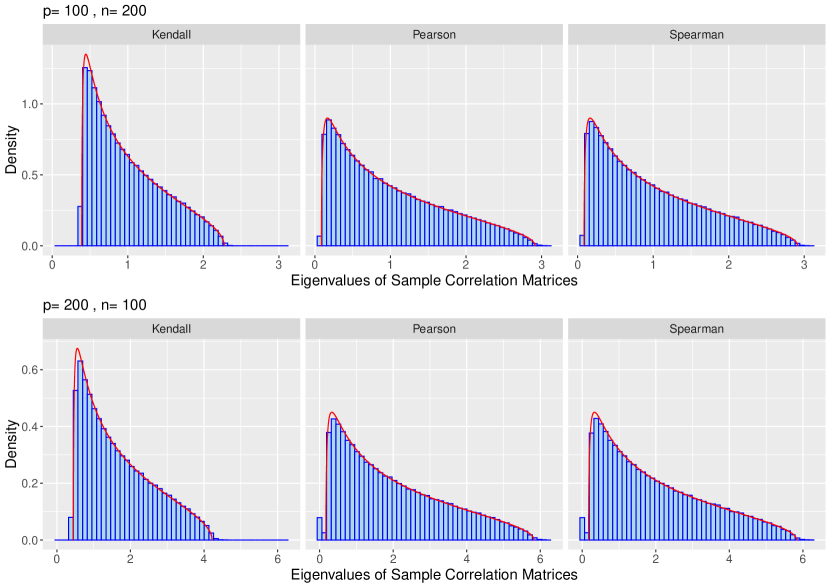
Figure 2: Histograms of eigenvalues of three types of sample correlation matrices, Kendall $\mathbf{K}_{n}$, Pearson $\mathbf{R}_{n}$, Spearman $\mathbf{S}_{n}$ for data sample $\mathbf{x}_{1},\cdots,\mathbf{x}_{n}\sim N_{p}(0,\mathbf{I}_{p})$ with $(p,n)=(100,200)$ and $(p,n)=(200,100)$. The red curves are density functions of their corresponding limiting spectral distribution.

Model (II):
The second case is the factor model or the spiked model, i.e., the population covariance matrix is

$$\mbox{cov}(\mathbf{x}_{t})=\mbox{\boldmath$\Sigma$}_{0}=\mathbf{I}_{p}+\mathbf{A}^{\mathrm{\scriptscriptstyle T}}\mathbf{A},$$

where $\mbox{rank}(\mathbf{A})\leq k$. For the related correlation matrix $\Sigma$, we have

$$\mbox{\boldmath$\Sigma$}=\mbox{diag}(\mbox{\boldmath$\Sigma$}_{0})^{-1/2}\cdot\mbox{\boldmath$\Sigma$}_{0}\cdot\mbox{diag}(\mbox{\boldmath$\Sigma$}_{0})^{-1/2}=\mbox{diag}(\mbox{\boldmath$\Sigma$}_{0})^{-1}+\tilde{\mathbf{A}}^{\mathrm{\scriptscriptstyle T}}\tilde{\mathbf{A}},$$

where $\tilde{\mathbf{A}}=\mathbf{A}\mbox{diag}(\mbox{\boldmath$\Sigma$}_{0})^{-1/2}$. Noting,

$$\mbox{\boldmath$\Sigma$}_{1}= \frac{2}{\pi}\arcsin(\mbox{\boldmath$\Sigma$}),~{}\mbox{\boldmath$\Sigma$}_{2}=\frac{2}{\pi}\arcsin(\mbox{\boldmath$\Sigma$}/2),~{}\mbox{\boldmath$\Sigma$}_{3}=\mbox{\boldmath$\Sigma$}_{1}-2\mbox{\boldmath$\Sigma$}_{2},$$

and $2x/\pi\leq 2\arcsin(x)/\pi\leq x$ for any $x\in[0,1]$, we have

$$\frac{1}{p}\left\|\mbox{\boldmath$\Sigma$}_{1}-\mathbf{I}_{p}\right\|_{2}^{2}\leq\frac{1}{p}\left\|\frac{2}{\pi}\arcsin(\tilde{\mathbf{A}}^{\mathrm{\scriptscriptstyle T}}\tilde{\mathbf{A}})\right\|_{2}^{2}\leq\frac{1}{p}\left\|\tilde{\mathbf{A}}^{\mathrm{\scriptscriptstyle T}}\tilde{\mathbf{A}}\right\|_{2}^{2}\leq\frac{1}{p}\left\|\mathbf{A}^{\mathrm{\scriptscriptstyle T}}\mathbf{A}\right\|_{2}^{2}$$

and

$$\frac{1}{p}\left\|\mbox{\boldmath$\Sigma$}_{2}-\frac{1}{3}\mathbf{I}_{p}\right\|_{2}^{2}\leq\frac{1}{p}\left\|\frac{2}{\pi}\arcsin(\tilde{\mathbf{A}}^{\mathrm{\scriptscriptstyle T}}\tilde{\mathbf{A}}/2)\right\|_{2}^{2}\leq\frac{1}{4p}\left\|\mathbf{A}^{\mathrm{\scriptscriptstyle T}}\mathbf{A}\right\|_{2}^{2}.$$

Thus, when

$$\frac{1}{p}\left\|\mathbf{A}^{\mathrm{\scriptscriptstyle T}}\mathbf{A}\right\|_{2}^{2}\to 0,$$

the LSD is still an affine transformation of Marc̆enko-Pastur law (Bandeira, Lodhia and Rigollet, 2017). If the term $\|\mathbf{A}^{\mathrm{\scriptscriptstyle T}}\mathbf{A}\|_{2}^{2}/p$ is large, the result violates the affine transformation of Marc̆enko-Pastur law. To demonstrate these results, we consider two covariance matrices:

$$\mbox{\boldmath$\Sigma$}_{0}=\mathbf{I}_{p}+\frac{1}{p}\mathbf{Z}^{\mathrm{\scriptscriptstyle T}}\mathbf{Z},~{}\mbox{and}~{}\mbox{\boldmath$\Sigma$}_{0}=\mathbf{I}_{p}+\frac{1}{\sqrt{p}}\mathbf{Z}^{\mathrm{\scriptscriptstyle T}}\mathbf{Z},$$

where $\mathbf{Z}=(Z_{ij})_{k\times p}$ and $Z_{ij}~{}i.i.d.\sim N(0,1)$. Figure 3 shows the results which are consistent with our analysis.

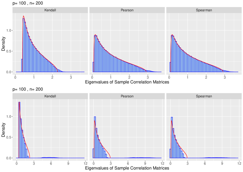
Figure 3: Histograms of eigenvalues of three types of sample correlation matrices, Kendall $\mathbf{K}_{n}$, Pearson $\mathbf{R}_{n}$, Spearman $\mathbf{S}_{n}$ for data sample $\mathbf{x}_{1},\cdots,\mathbf{x}_{n}\sim N_{p}(0,\mathbf{I}_{p}+\mathbf{Z}^{\mathrm{\scriptscriptstyle T}}\mathbf{Z}/p)$ in the upper panel and $\mathbf{x}_{1},\cdots,\mathbf{x}_{n}\sim N_{p}(0,\mathbf{I}_{p}+\mathbf{Z}^{\mathrm{\scriptscriptstyle T}}\mathbf{Z}/\sqrt{p})$ in the lower panel, $\mathbf{Z}=(Z_{ij})_{k\times p},~{}Z_{ij}\sim N(0,1)$ i.i.d. with $k=3$, $(p,n)=(100,200)$ and $(p,n)=(200,100)$. The red curves are density functions of the affine transformation of Marc̆enko-Pastur law.

Model (III):
As for MA(1) model, we focus on the spectral behavior of $\mathbf{K}_{n}$ since little is known about $\mathbf{S}_{n}$ and $\mathbf{R}_{n}$ in the dependent case. Similarly, we generate data sample $\mathbf{x}_{1},\ldots,\mathbf{x}_{n}\sim N(0,\mbox{\boldmath$\Sigma$})$ where $\Sigma$ follows MA(1) model (III) with $\rho=0.5$. The LSD are derived using Proposition 4.4 and the inversion formula (3.1). Then the histogram of eigenvalues of $\mathbf{K}_{n}$ under different combinations of $(p,n)$ are compared with their corresponding limiting densities in Figure  4. It can be seen from Figure 4 that the LSDs under MA(1) model are different from the independent case. All empirical histograms conform to our theoretical limits, which proves the accuracy of our theory.

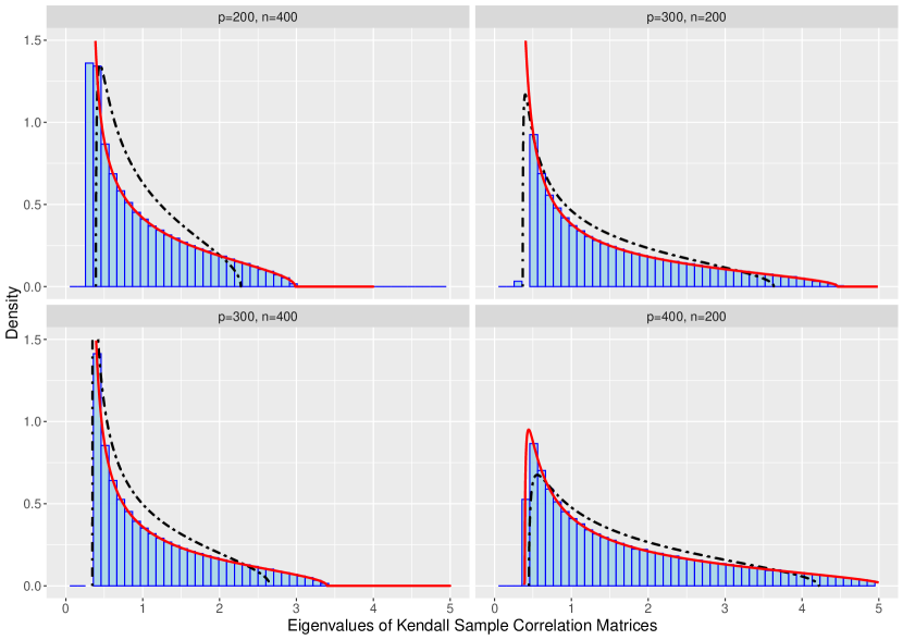
Figure 4: Histograms of eigenvalues of Kendall sample correlation matrices for data sample $\mathbf{x}_{1},\cdots,\mathbf{x}_{n}\sim N_{p}(0,\mbox{\boldmath$\Sigma$})$ where $\Sigma$ follows MA(1) Model (II) with $\rho=0.5$ for $(p,n)=(200,400)$, $(p,n)=(300,400)$, $(p,n)=(300,200)$ and $(p,n)=(400,200)$. The red curves are density functions of their corresponding limiting spectral distribution. The black dashed line are densities in the independent case for reference.

Model (IV):
As an illustration for the general Toeplitz matrix, we consider a band Toeplitz matrix with two parameters, i.e.,

$$\rho_{1}=\rho_{2}=\rho,~{}\rho_{k}=0,k=3,\cdots.$$

Noting

$$\mbox{\boldmath$\Sigma$}_{2}=\frac{2}{\pi}\arcsin(\mbox{\boldmath$\Sigma$}/2),~{}\mbox{\boldmath$\Sigma$}_{3}= \frac{2}{\pi}\arcsin(\mbox{\boldmath$\Sigma$})-\frac{4}{\pi}\arcsin(\mbox{\boldmath$\Sigma$}/2),$$

we have

$$\mbox{\boldmath$\Sigma$}_{3}-\frac{1}{3}\mathbf{I}_{p}=a(\mbox{\boldmath$\Sigma$}_{2}-\frac{1}{3}\mathbf{I}_{p}),~{}a=\frac{\arcsin(\rho)}{\arcsin(\rho/2)}-2$$

and then

$$\mbox{\boldmath$\Sigma$}_{3}=a\mbox{\boldmath$\Sigma$}_{2}+\frac{1-a}{3}\mathbf{I}_{p}.$$

The assumption (3.3) is

$$\lim_{p\to\infty}\frac{1}{p}\mbox{tr}\big{[}((2x+a)\mbox{\boldmath$\Sigma$}_{2}-(z-\frac{1-a}{3})\mathbf{I}_{p})^{-1}\mbox{\boldmath$\Sigma$}_{2}\big{]}=\frac{1-x}{2cx}.$$

and Proposition 4.5 yields

$$\frac{1-x}{2cx}=\frac{1}{2\pi}\int_{0}^{2\pi}\frac{f_{2}(\theta)}{(2x+a)f_{2}(\theta)-(z-\frac{1-a}{3})}d\theta$$ (5.1)

where

$$f_{2}(\theta)= \frac{1}{3}+\frac{4}{\pi}\arcsin\frac{\rho}{2}\big{[}\cos{(\theta)}+\cos{(2\theta)}\big{]}.$$

Solving (5.1) to get $x(z)$, the Stieltjes transform of the LSD (3.5) is

$$s(z)= \lim_{p\to\infty}\frac{1}{p}\mbox{tr}\left((2x+a)\mbox{\boldmath$\Sigma$}_{2}-(z-\frac{1-a}{3})\mathbf{I}_{p}\right)^{-1}$$

$$= -\frac{1}{z_{1}}\lim_{p\to\infty}\frac{1}{p}\mbox{tr}\left((2x+a)\mbox{\boldmath$\Sigma$}_{2}-z_{1}\mathbf{I}_{p}\right)^{-1}\left((2x+a)\mbox{\boldmath$\Sigma$}_{2}-z_{1}\mathbf{I}_{p}-(2x+a)\mbox{\boldmath$\Sigma$}_{2}\right)$$

$$= -\frac{1}{z_{1}}\left(1-\frac{(2x+a)(1-x)}{2cx}\right)=\frac{(2x+a)(1-x)-2cx}{2cz_{1}x},$$

where

$$z_{1}=z-\frac{1-a}{3}.$$

Figure 5 shows the results with $\rho=0.25$ and again, we can see that the empirical histogram conforms to our theoretical result.

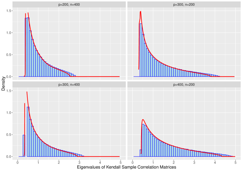
Figure 5: Histograms of eigenvalues of Kendall sample correlation matrices for data sample $\mathbf{x}_{1},\cdots,\mathbf{x}_{n}\sim N_{p}(0,\mbox{\boldmath$\Sigma$})$ where $\Sigma$ follows general Toeplitz Model (IV) with $\rho=0.25$ for $(p,n)=(200,400)$, $(p,n)=(300,400)$, $(p,n)=(300,200)$ and $(p,n)=(400,200)$. The red curves are density functions of their corresponding limiting spectral distribution.

Appendix

This Appendix contains all supporting lemmas and proofs.

A1 Proof of Proposition 2.2

The following results show that $\mathbf{M}_{2}$ and $\mathbf{M}_{3}$ are concentrated on their population means, respectively.

Lemma A1.1.

Under the assumption of Proposition 2.2,

$$\frac{1}{p}\mathbb{E}\|\mathbf{M}_{2}\|_{2}^{2}\leq\frac{4p^{2}}{3np(n-1)}+\frac{{8}}{np}\mbox{tr}(\mbox{\boldmath$\Sigma$}^{2}_{2})\to 0.$$

Lemma A1.2.

Under the assumption of Proposition2.2,

$$\frac{1}{p}\mathbb{E}\|\mathbf{M}_{3}-\mbox{\boldmath$\Sigma$}_{3}\|_{2}^{2}\leq\frac{2p^{2}}{3np(n-1)}+\frac{32}{np}\mbox{tr}\{\mbox{\boldmath$\Sigma$}_{1}(\mbox{\boldmath$\Sigma$}_{1}+\mbox{\boldmath$\Sigma$}_{2})\}\to 0.$$

Equipped with these two results, we are now ready to prove Proposition 2.2. By the Corollary A.41 of Bai and Silverstein (2010),

$$L^{3}(F^{\mathbf{K}_{n}},F^{\mathbf{W}_{n}})\leq\frac{1}{p}\|\mathbf{K}_{n}-\mathbf{W}_{n}\|_{2}^{2}\leq\frac{6}{p}\|\mathbf{M}_{2}\|_{2}^{2}+\frac{3}{p}\|\mathbf{M}_{3}-\mbox{\boldmath$\Sigma$}_{3}\|_{2}^{2}$$

which yields

$$\mathbb{E}L^{3}(F^{\mathbf{K}_{n}},F^{\mathbf{W}_{n}})\to 0.$$

The proof is completed.

It remains to prove the two auxiliary Lemmas A1.1 and A1.2.

A1.1 Proof of Lemma A1.1

Writing the kernel function

$$\mathbf{h}(i,j)=(\mathbf{A}_{i}-\mathbf{A}_{j})(\mathbf{A}_{ij}-\mathbf{A}_{i}+\mathbf{A}_{j})^{\mathrm{\scriptscriptstyle T}},$$

we have

$$\mathbf{M}_{2} =\frac{2}{n(n-1)}\sum_{1\leq i<j\leq n}(\mathbf{A}_{i}-\mathbf{A}_{j})(\mathbf{A}_{ij}-\mathbf{A}_{i}+\mathbf{A}_{j})^{\mathrm{\scriptscriptstyle T}}$$

$$=\frac{2}{n(n-1)}\sum_{1\leq i<j\leq n}\mathbf{h}(i,j).$$

For the kernel function, we have the following properties.

• For the mean parts,

  $$\mathbf{h}(i,j)=\mathbf{h}(j,i),\quad\mathbb{E}\mathbf{h}(1,2)=\mathbf{0},\quad\mathbb{E}\left[\mathbf{h}(1,2)|\mathbf{x}_{1}\right]=-\mathbb{E}\left[\mathbf{A}_{2}\mathbf{A}_{12}^{\mathrm{\scriptscriptstyle T}}|\mathbf{x}_{1}\right]-\mbox{\boldmath$\Sigma$}_{2}.$$

• For the Frobenius norm of the kernel function, we have

  $$\mathbb{E}\mbox{tr}(\mathbf{h}(1,2)^{\mathrm{\scriptscriptstyle T}}\mathbf{h}(1,2))=\mathbb{E}\left(\|\mathbf{A}_{12}-\mathbf{A}_{1}+\mathbf{A}_{2}\|_{2}^{2}\|\mathbf{A}_{1}-\mathbf{A}_{2}\|_{2}^{2}\right).$$

  Since

  $$\|\mathbf{A}_{12}-\mathbf{A}_{1}+\mathbf{A}_{2}\|_{\infty}= \|\mbox{sign}(\mathbf{A}_{1}-\mathbf{A}_{2})-(\mathbf{A}_{1}-\mathbf{A}_{2})\|_{\infty}\leq 1,$$

  and $\|\mathbf{A}_{i}\|_{\infty}\leq 1$, we have

  $$\|\mathbf{A}_{12}-\mathbf{A}_{1}+\mathbf{A}_{2}\|_{2}^{2}\leq p,\mbox{and}\quad\|\mathbf{A}_{1}-\mathbf{A}_{2}\|_{2}^{2}\leq 4p,$$

  which yields

  $$\mathbb{E}\mbox{tr}(\mathbf{h}(1,2)^{\mathrm{\scriptscriptstyle T}}\mathbf{h}(1,2))\leq 4p^{2}.$$

• For the the Frobenius norm of the conditional mean, we have

  $$\mathbb{E}\mbox{tr}(\mathbf{h}(1,2)^{\mathrm{\scriptscriptstyle T}}\mathbf{h}(1,3))= \mbox{tr}\{\mathbb{E}(\mathbf{A}_{2}\mathbf{A}_{12}^{\mathrm{\scriptscriptstyle T}}+\mbox{\boldmath$\Sigma$}_{2})^{\mathrm{\scriptscriptstyle T}}(\mathbf{A}_{3}\mathbf{A}_{13}^{\mathrm{\scriptscriptstyle T}}+\mbox{\boldmath$\Sigma$}_{2})\}$$

  $$= \mbox{cov}(\mathbf{A}_{13}^{\mathrm{\scriptscriptstyle T}}\mathbf{A}_{12},\mathbf{A}_{2}^{\mathrm{\scriptscriptstyle T}}\mathbf{A}_{3})-\mbox{tr}(\mbox{\boldmath$\Sigma$}^{2}_{2})$$

  $$\leq \mathbb{E}|\mathbf{A}_{13}^{\mathrm{\scriptscriptstyle T}}\mathbf{A}_{12}||\mathbf{A}_{2}^{\mathrm{\scriptscriptstyle T}}\mathbf{A}_{3}|\leq p\cdot\{\mbox{var}(\mathbf{A}_{3}^{\mathrm{\scriptscriptstyle T}}\mathbf{A}_{2})\}^{1/2}$$

  $$= p\cdot\{\ \mbox{tr}(\mbox{\boldmath$\Sigma$}^{2}_{2})\}^{1/2}\leq p^{3/2}\cdot\|\mbox{\boldmath$\Sigma$}_{2}\|\leq p^{3/2}\cdot\|\mbox{\boldmath$\Sigma$}_{1}\|.$$

  which yields

  $$\mathbb{E}\mbox{tr}(\mathbf{h}(1,2)^{\mathrm{\scriptscriptstyle T}}\mathbf{h}(1,3))\leq Cp^{3/2}.$$

Putting together the pieces, we conclude that

$$\frac{1}{p}\mathbb{E}\left(\mathbf{M}_{2}^{\mathrm{\scriptscriptstyle T}}\mathbf{M}_{2}\right)=\frac{1}{p} \mathbb{E}\bigg{\{}\frac{2}{n(n-1)}\sum_{1\leq i<j\leq n}\mathbf{h}(i,j)\bigg{\}}^{\mathrm{\scriptscriptstyle T}}\bigg{\{}\frac{2}{n(n-1)}\sum_{1\leq k<l\leq n}\mathbf{h}(k,l)\bigg{\}}$$

$$= \frac{2}{np(n-1)}\mathbb{E}\mbox{tr}(\mathbf{h}(1,2)^{\mathrm{\scriptscriptstyle T}}\mathbf{h}(1,2))+\frac{4p(n-2)}{n(n-1)}\mathbb{E}\mbox{tr}(\mathbf{h}(1,2)^{\mathrm{\scriptscriptstyle T}}\mathbf{h}(1,3))$$

$$\leq \frac{8p^{2}}{np(n-1)}+\frac{4Cp^{3/2}}{np}\to 0.$$

The proof is completed.

A1.2 Proof of Lemma A1.2

Recalling

$$\mathbf{M}_{3}=\frac{2}{n(n-1)}\sum_{1\leq i<j\leq n}\epsilon_{ij}\epsilon_{ij}^{\mathrm{\scriptscriptstyle T}},$$

we have

$$\mathbb{E}\mbox{tr}\{(\mathbf{M}_{3}-\mbox{\boldmath$\Sigma$}_{3})(\mathbf{M}_{3}-\mbox{\boldmath$\Sigma$}_{3})^{\mathrm{\scriptscriptstyle T}}\}$$

$$= ~{}\frac{4}{n^{2}(n-1)^{2}}\sum_{i<j,k<l}\mathbb{E}\{\epsilon_{kl}^{\mathrm{\scriptscriptstyle T}}(\epsilon_{ij}\epsilon_{ij}^{\mathrm{\scriptscriptstyle T}}-\mbox{\boldmath$\Sigma$}_{3})\epsilon_{kl}\}$$

$$= ~{}\frac{2}{n(n-1)}\mathbb{E}\{\epsilon_{12}^{\mathrm{\scriptscriptstyle T}}(\epsilon_{12}\epsilon_{12}^{\mathrm{\scriptscriptstyle T}}-\mbox{\boldmath$\Sigma$}_{3})\epsilon_{12}\}+\frac{4(n-2)}{{n(n-1)}}\mathbb{E}\{\epsilon_{12}^{\mathrm{\scriptscriptstyle T}}(\epsilon_{13}\epsilon_{13}^{\mathrm{\scriptscriptstyle T}}-\mbox{\boldmath$\Sigma$}_{3})\epsilon_{12}\}$$

$$= ~{}\frac{2}{n(n-1)}\{\mathbb{E}(\epsilon_{12}^{\mathrm{\scriptscriptstyle T}}\epsilon_{12})^{2}-\mbox{tr}(\mbox{\boldmath$\Sigma$}^{2}_{3})\}+\frac{4(n-2)}{{n(n-1)}}\{\mathbb{E}(\epsilon_{12}^{\mathrm{\scriptscriptstyle T}}\epsilon_{13})^{2}-\mbox{tr}(\mbox{\boldmath$\Sigma$}^{2}_{3})\}$$

$$\leq ~{}\frac{2}{n(n-1)}\mathbb{E}(\epsilon_{12}^{\mathrm{\scriptscriptstyle T}}\epsilon_{12})^{2}+\frac{4}{{n}}\mathbb{E}(\epsilon_{12}^{\mathrm{\scriptscriptstyle T}}\epsilon_{13})^{2}.$$

For the first term, we have

$$\epsilon_{12}^{\mathrm{\scriptscriptstyle T}}\epsilon_{12}=\|\mathbf{A}_{12}-\mathbf{A}_{1}+\mathbf{A}_{2}\|_{2}^{2}\leq p\|\mathbf{A}_{12}-\mathbf{A}_{1}+\mathbf{A}_{2}\|_{\infty}^{2}\leq p,$$

which yields $\mathbb{E}(\epsilon_{12}^{\mathrm{\scriptscriptstyle T}}\epsilon_{12})^{2}\leq p^{2}$. For the second term, we have

$$(\epsilon_{12}^{\mathrm{\scriptscriptstyle T}}\epsilon_{13})^{2}=\{(\mathbf{A}_{12}-\mathbf{A}_{1}+\mathbf{A}_{2})^{\mathrm{\scriptscriptstyle T}}(\mathbf{A}_{13}-\mathbf{A}_{1}+\mathbf{A}_{3})\}^{2}$$

$$= ~{}\{(\mathbf{A}_{12}-\mathbf{A}_{1})^{\mathrm{\scriptscriptstyle T}}(\mathbf{A}_{13}-\mathbf{A}_{1})+\mathbf{A}_{2}^{\mathrm{\scriptscriptstyle T}}(\mathbf{A}_{13}-\mathbf{A}_{1})+\mathbf{A}_{3}^{\mathrm{\scriptscriptstyle T}}(\mathbf{A}_{12}-\mathbf{A}_{1})+\mathbf{A}_{2}^{\mathrm{\scriptscriptstyle T}}\mathbf{A}_{3}\}^{2}$$

$$\leq ~{}4\{(\mathbf{A}_{12}-\mathbf{A}_{1})^{\mathrm{\scriptscriptstyle T}}(\mathbf{A}_{13}-\mathbf{A}_{1})\}^{2}+4\{\mathbf{A}_{2}^{\mathrm{\scriptscriptstyle T}}(\mathbf{A}_{13}-\mathbf{A}_{1})\}^{2}+4\{\mathbf{A}_{3}^{\mathrm{\scriptscriptstyle T}}(\mathbf{A}_{12}-\mathbf{A}_{1})\}^{2}+4(\mathbf{A}_{2}^{\mathrm{\scriptscriptstyle T}}\mathbf{A}_{3})^{2},$$

and

$$\frac{1}{4}\mathbb{E}(\epsilon_{12}^{\mathrm{\scriptscriptstyle T}}\epsilon_{13})^{2}\leq \mathbb{E}\{(\mathbf{A}_{12}-\mathbf{A}_{1})^{\mathrm{\scriptscriptstyle T}}(\mathbf{A}_{13}-\mathbf{A}_{1})\}^{2}+\mathbb{E}\{\mathbf{A}_{2}^{\mathrm{\scriptscriptstyle T}}(\mathbf{A}_{13}-\mathbf{A}_{1})\}^{2}$$

$$+\mathbb{E}\{\mathbf{A}_{3}^{\mathrm{\scriptscriptstyle T}}(\mathbf{A}_{12}-\mathbf{A}_{1})\}^{2}+\mathbb{E}(\mathbf{A}_{2}^{\mathrm{\scriptscriptstyle T}}\mathbf{A}_{3})^{2}$$

$$= \mathbb{E}\{(\mathbf{A}_{12}-\mathbf{A}_{1})^{\mathrm{\scriptscriptstyle T}}\mathbf{A}_{13}\}^{2}-\mathbb{E}\{(\mathbf{A}_{12}-\mathbf{A}_{1})^{\mathrm{\scriptscriptstyle T}}\mathbf{A}_{1}\}^{2}+2\mbox{tr}\{\mbox{\boldmath$\Sigma$}_{2}(\mbox{\boldmath$\Sigma$}_{1}-\mbox{\boldmath$\Sigma$}_{2})\}+\mbox{tr}\{\mbox{\boldmath$\Sigma$}_{2}^{2}\}$$

$$\leq \mathbb{E}\{(\mathbf{A}_{12}-\mathbf{A}_{1})^{\mathrm{\scriptscriptstyle T}}\mathbf{A}_{13}\}^{2}+2\mbox{tr}\{\mbox{\boldmath$\Sigma$}_{1}\mbox{\boldmath$\Sigma$}_{2}\}=\mbox{var}(\mathbf{A}_{12}^{\mathrm{\scriptscriptstyle T}}\mathbf{A}_{13})-\mbox{var}(\mathbf{A}_{12}^{\mathrm{\scriptscriptstyle T}}\mathbf{A}_{1})+2\mbox{tr}\{\mbox{\boldmath$\Sigma$}_{1}\mbox{\boldmath$\Sigma$}_{2}\}$$

$$\leq \mbox{var}(\mathbf{A}_{12}^{\mathrm{\scriptscriptstyle T}}\mathbf{A}_{13})+2pC^{2}.$$

Finally, we have

$$\frac{1}{p}\mathbb{E}\mbox{tr}\{(\mathbf{M}_{3}-\mbox{\boldmath$\Sigma$}_{3})(\mathbf{M}_{3}-\mbox{\boldmath$\Sigma$}_{3})^{\mathrm{\scriptscriptstyle T}}\}\leq\frac{2p^{2}}{np(n-1)}+\frac{16}{np}\mbox{var}(\mathbf{A}_{12}^{\mathrm{\scriptscriptstyle T}}\mathbf{A}_{13})+\frac{32}{np}pC^{2}\to 0.$$

The proof is completed.

A2 Proof of Theorem 3.1

According to Proposition 2.2, it suffices to study the LSD of the following matrix $\mathbf{M}_{n}$.

$$\mathbf{M}_{n}=\frac{2}{n}\sum_{i=1}^{n}\mathbf{A}_{i}\mathbf{A}_{i}^{\mathrm{\scriptscriptstyle T}}+\mbox{\boldmath$\Sigma$}_{3}.$$ (A.1)

Let $s_{n}(z)$ be the Stieltjes transform of $F^{\mathbf{M}_{n}}$, then the convergence of $F^{\mathbf{M}_{n}}$ can be determined in three steps:

• Step 1: For any fixed $z\in\mathbb{C}^{+}$, $s_{n}(z)-\mathbb{E}s_{n}(z)\to 0$, almost surely.

• Step 2: For any fixed $z\in\mathbb{C}^{+}$, $\mathbb{E}s_{n}(z)\to s(z)$ with $s(z)$ satisfies the equations in (3.5).

• Step 3: The uniqueness of the solution $s(z)$ to (3.5) on the set $\mathbb{C}^{+}$.

A2.1 Almost sure convergence of $s_{n}(z)-\mathbb{E}s_{n}(z)$

Denote

$$\mathbf{M}_{n,k}=\frac{2}{n}\sum_{i\neq k}^{n}\mathbf{A}_{i}\mathbf{A}_{i}^{\mathrm{\scriptscriptstyle T}}+\mbox{\boldmath$\Sigma$}_{3}.$$

Let $\mathbb{E}_{0}(\cdot)$ be expectation and $\mathbb{E}_{k}(\cdot)$ be conditional expectation given $\mathbf{A}_{1},\ldots,\mathbf{A}_{k}$. From the martingale decomposition and the identity

$$(\mathbf{M}_{n}-z\mathbf{I}_{p})^{-1}\mathbf{A}_{k}=\frac{(\mathbf{M}_{n,k}-z\mathbf{I}_{p})^{-1}\mathbf{A}_{k}}{1+2n^{-1}\mathbf{A}_{k}^{\mathrm{\scriptscriptstyle T}}(\mathbf{M}_{n,k}-z\mathbf{I}_{p})^{-1}\mathbf{A}_{k}},$$ (A.2)

we have

$$s_{n}(z)-\mathbb{E}s_{n}(z)= \frac{1}{p}\sum_{k=1}^{n}(\mathbb{E}_{k}-\mathbb{E}_{k-1})\left[\mbox{tr}(\mathbf{M}_{n}-z\mathbf{I}_{p})^{-1}-\mbox{tr}(\mathbf{M}_{n,k}-z\mathbf{I}_{p})^{-1}\right]$$

$$= -\frac{1}{p}\sum_{k=1}^{n}(\mathbb{E}_{k}-\mathbb{E}_{k-1})\frac{2n^{-1}\mathbf{A}_{k}^{\mathrm{\scriptscriptstyle T}}(\mathbf{M}_{n,k}-z\mathbf{I}_{p})^{-2}\mathbf{A}_{k}}{1+2n^{-1}\mathbf{A}_{k}^{\mathrm{\scriptscriptstyle T}}(\mathbf{M}_{n,k}-z\mathbf{I}_{p})^{-1}\mathbf{A}_{k}}$$

$$\stackrel{{\scriptstyle\mbox{{\tiny def}}}}{{=}} -\frac{1}{p}\sum_{k=1}^{n}(\mathbb{E}_{k}-\mathbb{E}_{k-1})r_{k}.$$

Since

$$|r_{k}|\leq\frac{\left|2n^{-1}\mathbf{A}_{k}^{\mathrm{\scriptscriptstyle T}}(\mathbf{M}_{n,k}-z\mathbf{I}_{p})^{-2}\mathbf{A}_{k}\right|}{\left|\Im(1+2n^{-1}\mathbf{A}_{k}^{\mathrm{\scriptscriptstyle T}}(\mathbf{M}_{n,k}-z\mathbf{I}_{p})^{-1}\mathbf{A}_{k})\right|}\leq\frac{1}{\Im(z)},$$

$\{(\mathbb{E}_{k}-\mathbb{E}_{k-1})r_{k}\}$ forms a bounded martingale difference sequence. Hence for any $\ell>1$,

$$\mathbb{E}|s_{n}(z)-\mathbb{E}s_{n}(z)|^{\ell} \leq Kp^{-\ell}\mathbb{E}\bigg{(}\sum_{k=1}^{n}\big{|}(\mathbb{E}_{k}-\mathbb{E}_{k-1})r_{k}\big{|}^{2}\bigg{)}^{\ell/2}$$

$$\leq Kp^{-\frac{\ell}{2}}\Im(z)^{-\ell},$$ (A.3)

which implies $s_{n}(z)-\mathbb{E}s_{n}(z)\to 0$, almost surely.

A2.2 Convergence of $\mathbb{E}s_{n}(z)$

Denote

$$x_{n}=x_{n}(z)=\frac{1}{n}\sum_{k=1}^{n}\frac{1}{1+2n^{-1}\mathbb{E}\left[\mbox{tr}\left\{(\mathbf{M}_{n,k}-z\mathbf{I}_{p})^{-1}\mbox{\boldmath$\Sigma$}_{2}\right\}\right]}.$$ (A.4)

Starting from the identity

$$\quad\left(2x_{n}\mbox{\boldmath$\Sigma$}_{2}+\mbox{\boldmath$\Sigma$}_{3}-z\mathbf{I}_{p}\right)^{-1}-(\mathbf{M}_{n}-z\mathbf{I}_{p})^{-1}$$

$$=\left(2x_{n}\mbox{\boldmath$\Sigma$}_{2}+\mbox{\boldmath$\Sigma$}_{3}-z\mathbf{I}_{p}\right)^{-1}\bigg{(}\frac{2}{n}\sum_{k=1}^{n}\mathbf{A}_{k}\mathbf{A}_{k}-2x_{n}\mbox{\boldmath$\Sigma$}_{2}\bigg{)}(\mathbf{M}_{n}-z\mathbf{I}_{p})^{-1},$$

then take trace on both sides and by (A.2), we have

$$~{}\quad\frac{1}{p}\mbox{tr}(2x_{n}\mbox{\boldmath$\Sigma$}_{2}+\mbox{\boldmath$\Sigma$}_{3}-z\mathbf{I}_{p})^{-1}-s_{n}(z)$$

$$=\frac{2}{np}\sum_{k=1}^{n}\frac{\mathbf{A}_{k}^{\mathrm{\scriptscriptstyle T}}(\mathbf{M}_{n,k}-z\mathbf{I}_{p})^{-1}(2x_{n}\mbox{\boldmath$\Sigma$}_{2}+\mbox{\boldmath$\Sigma$}_{3}-z\mathbf{I}_{p})^{-1}\mathbf{A}_{k}}{1+2n^{-1}\mathbf{A}_{k}^{\mathrm{\scriptscriptstyle T}}(\mathbf{M}_{n,k}-z\mathbf{I}_{p})^{-1}\mathbf{A}_{k}}$$ (A.5)

$$\quad-\frac{2x_{n}}{p}\mbox{tr}\left\{(2x_{n}\mbox{\boldmath$\Sigma$}_{2}+\mbox{\boldmath$\Sigma$}_{3}-z\mathbf{I}_{p})^{-1}\mbox{\boldmath$\Sigma$}_{2}(\mathbf{M}_{n}-z\mathbf{I}_{p})^{-1}\right\}$$

$$\stackrel{{\scriptstyle\mbox{{\tiny def}}}}{{=}}\frac{2}{n}\sum_{k=1}^{n}\frac{d_{k}}{1+2n^{-1}\mathbb{E}\left[\mbox{tr}\left\{(\mathbf{M}_{n,k}-z\mathbf{I}_{p})^{-1}\mbox{\boldmath$\Sigma$}_{2}\right\}\right]},$$ (A.6)

where

$$d_{k} =\frac{1+2n^{-1}\mathbb{E}\left[\mbox{tr}\left\{(\mathbf{M}_{n,k}-z\mathbf{I}_{p})^{-1}\mbox{\boldmath$\Sigma$}_{2}\right\}\right]}{1+2n^{-1}\mathbf{A}_{k}^{\mathrm{\scriptscriptstyle T}}(\mathbf{M}_{n,k}-z\mathbf{I}_{p})^{-1}\mathbf{A}_{k}}\cdot\frac{1}{p}\mathbf{A}_{k}^{\mathrm{\scriptscriptstyle T}}(\mathbf{M}_{n,k}-z\mathbf{I}_{p})^{-1}(2x_{n}\mbox{\boldmath$\Sigma$}_{2}+\mbox{\boldmath$\Sigma$}_{3}-z\mathbf{I}_{p})^{-1}\mathbf{A}_{k}$$

$$\quad\quad-\frac{1}{p}\mbox{tr}\left\{(\mathbf{M}_{n}-z\mathbf{I}_{p})^{-1}(2x_{n}\mbox{\boldmath$\Sigma$}_{2}+\mbox{\boldmath$\Sigma$}_{3}-z\mathbf{I}_{p})^{-1}\mbox{\boldmath$\Sigma$}_{2}\right\}.$$

We decompose

$$d_{k}\stackrel{{\scriptstyle\mbox{{\tiny def}}}}{{=}}d_{k1}+d_{k2}+d_{k3},$$

where

$$d_{k1} =\frac{1}{p}\mbox{tr}\left\{(\mathbf{M}_{n,k}-z\mathbf{I}_{p})^{-1}(2x_{n}\mbox{\boldmath$\Sigma$}_{2}+\mbox{\boldmath$\Sigma$}_{3}-z\mathbf{I}_{p})^{-1}\mbox{\boldmath$\Sigma$}_{2}\right\}$$

$$\quad-\frac{1}{p}\mbox{tr}\left\{(\mathbf{M}_{n}-z\mathbf{I}_{p})^{-1}(2x_{n}\mbox{\boldmath$\Sigma$}_{2}+\mbox{\boldmath$\Sigma$}_{3}-z\mathbf{I}_{p})^{-1}\mbox{\boldmath$\Sigma$}_{2}\right\},$$

$$d_{k2} =\frac{1}{p}\mathbf{A}_{k}^{\mathrm{\scriptscriptstyle T}}(\mathbf{M}_{n,k}-z\mathbf{I}_{p})^{-1}(2x_{n}\mbox{\boldmath$\Sigma$}_{2}+\mbox{\boldmath$\Sigma$}_{3}-z\mathbf{I}_{p})^{-1}\mathbf{A}_{k}$$

$$\quad-\frac{1}{p}\mbox{tr}\left\{(\mathbf{M}_{n,k}-z\mathbf{I}_{p})^{-1}(2x_{n}\mbox{\boldmath$\Sigma$}_{2}+\mbox{\boldmath$\Sigma$}_{3}-z\mathbf{I}_{p})^{-1}\mbox{\boldmath$\Sigma$}_{2}\right\},$$

$$d_{k3} =\frac{-2\mathbf{A}_{k}^{\mathrm{\scriptscriptstyle T}}(\mathbf{M}_{n,k}-z\mathbf{I}_{p})^{-1}(2x_{n}\mbox{\boldmath$\Sigma$}_{2}+\mbox{\boldmath$\Sigma$}_{3}-z\mathbf{I}_{p})^{-1}\mathbf{A}_{k}}{pn\left\{1+2n^{-1}\mathbf{A}_{k}^{\mathrm{\scriptscriptstyle T}}(\mathbf{M}_{n,k}-z\mathbf{I}_{p})^{-1}\mathbf{A}_{k}\right\}}$$

$$\quad\times\bigg{\{}\mathbf{A}_{k}^{\mathrm{\scriptscriptstyle T}}(\mathbf{M}_{n,k}-z\mathbf{I}_{p})^{-1}\mathbf{A}_{k}-\mathbb{E}\big{[}\mbox{tr}\left\{(\mathbf{M}_{n,k}-z\mathbf{I}_{p})^{-1}\mbox{\boldmath$\Sigma$}_{2}\right\}\big{]}\bigg{\}}.$$

For the term $d_{k1}$, we have

$$|d_{k1}| =\left|\frac{2}{pn}\mbox{tr}\left\{(\mathbf{M}_{n}-z\mathbf{I}_{p})^{-1}\mathbf{A}_{k}\mathbf{A}_{k}^{\mathrm{\scriptscriptstyle T}}(\mathbf{M}_{n,k}-z\mathbf{I}_{p})^{-1}(2x_{n}\mbox{\boldmath$\Sigma$}_{2}+\mbox{\boldmath$\Sigma$}_{3}-z\mathbf{I}_{p})^{-1}\mbox{\boldmath$\Sigma$}_{2}\right\}\right|$$

$$=\left|\frac{2n^{-1}p^{-1}\mathbf{A}_{k}^{\mathrm{\scriptscriptstyle T}}(\mathbf{M}_{n,k}-z\mathbf{I}_{p})^{-1}(2x_{n}\mbox{\boldmath$\Sigma$}_{2}+\mbox{\boldmath$\Sigma$}_{3}-z\mathbf{I}_{p})^{-1}\mbox{\boldmath$\Sigma$}_{2}(\mathbf{M}_{n,k}-z\mathbf{I}_{p})^{-1}\mathbf{A}_{k}}{1+2n^{-1}\mathbf{A}_{k}^{\mathrm{\scriptscriptstyle T}}(\mathbf{M}_{n,k}-z\mathbf{I}_{p})^{-1}\mathbf{A}_{k}}\right|$$

$$\leq Kp^{-1}\Im(z)^{-2},$$ (A.7)

then its contribution to (A2.2) can be bounded as

$$\left|\frac{2}{n}\sum_{k=1}^{n}\frac{d_{k1}}{1+2n^{-1}\mathbb{E}\big{[}\mbox{tr}\left\{(\mathbf{M}_{n,k}-z\mathbf{I}_{p})^{-1}\mbox{\boldmath$\Sigma$}_{2}\right\}\big{]}}\right| \leq\frac{2}{n}\sum_{k=1}^{n}\frac{|d_{k1}|}{\Big{|}1+2n^{-1}\mathbb{E}\big{[}\mbox{tr}\left\{(\mathbf{M}_{n,k}-z\mathbf{I}_{p})^{-1}\mbox{\boldmath$\Sigma$}_{2}\right\}\big{]}\Big{|}}$$

$$\leq Kp^{-1}\Im(z)^{-2}\to 0.$$

For the term $d_{k2}$, we have

$$\mathbb{E}(d_{k2})=0.$$ (A.8)

For the term $d_{k3}$, we have the first part bounded by

$$\left|\frac{-2\mathbf{A}_{k}^{\mathrm{\scriptscriptstyle T}}(\mathbf{M}_{n,k}-z\mathbf{I}_{p})^{-1}(2x_{n}\mbox{\boldmath$\Sigma$}_{2}+\mbox{\boldmath$\Sigma$}_{3}-z\mathbf{I}_{p})^{-1}\mathbf{A}_{k}}{pn\left\{1+2n^{-1}\mathbf{A}_{k}^{\mathrm{\scriptscriptstyle T}}(\mathbf{M}_{n,k}-z\mathbf{I}_{p})^{-1}\mathbf{A}_{k}\right\}}\right|\leq Kp^{-1}n^{-1}\Im(z)^{-2}||\mathbf{A}_{k}||^{2}.$$

So we have

$$|\mathbb{E}(d_{k3})|^{2}\leq Kp^{-2}n^{-2}\mathbb{E}||\mathbf{A}_{k}||^{4}\mathbb{E}\Big{|}\mathbf{A}_{k}^{\mathrm{\scriptscriptstyle T}}(\mathbf{M}_{n,k}-z\mathbf{I}_{p})^{-1}\mathbf{A}_{k}-\mathbb{E}\big{[}\mbox{tr}\left\{(\mathbf{M}_{n,k}-z\mathbf{I}_{p})^{-1}\mbox{\boldmath$\Sigma$}_{2}\right\}\big{]}\Big{|}^{2}.$$

According to Lemma A3.2 and Lemma A3.3,

$$\mathbb{E}||\mathbf{A}_{k}||^{4}=\mbox{var}(\mathbf{A}_{k}^{\mathrm{\scriptscriptstyle T}}\mathbf{A}_{k})+\{\mathbb{E}(\mathbf{A}_{k}^{\mathrm{\scriptscriptstyle T}}\mathbf{A}_{k})\}^{2}\leq\mbox{tr}(\mbox{\boldmath$\Sigma$}_{1}^{2})-\mbox{tr}(\mbox{\boldmath$\Sigma$}_{2}^{2})+\{\mbox{tr}(\mbox{\boldmath$\Sigma$}_{2})\}^{2}=O(p^{2}),$$

$$\mathbb{E}\Big{|}\mathbf{A}_{k}^{\mathrm{\scriptscriptstyle T}}(\mathbf{M}_{n,k}-z\mathbf{I}_{p})^{-1}\mathbf{A}_{k}-\mathbb{E}\big{[}\mbox{tr}\left\{(\mathbf{M}_{n,k}-z\mathbf{I}_{p})^{-1}\mbox{\boldmath$\Sigma$}_{2}\right\}\big{]}\Big{|}^{2}$$

$$\quad\leq 3||\mbox{\boldmath$\Sigma$}||\cdot\mathbb{E}\big{[}\mbox{tr}\left\{(\mathbf{M}_{n,k}-z\mathbf{I}_{p})^{-2}\mbox{\boldmath$\Sigma$}_{2}\right\}\big{]}=O(p),$$

which gives

$$|\mathbb{E}(d_{k3})|^{2}\leq Kp^{-1}.$$ (A.9)

Combining (A2.2), (A2.2), (A.8) and (A.9), we have

$$\mathbb{E}s_{n}(z)\to\frac{1}{p}\mbox{tr}(2x\mbox{\boldmath$\Sigma$}_{2}+\mbox{\boldmath$\Sigma$}_{3}-z\mathbf{I}_{p})^{-1}\stackrel{{\scriptstyle\mbox{{\tiny def}}}}{{=}}s(z),$$ (A.10)

where $x$ is the limit of $x_{n}$.

Next, we give the equation that $x$ satisfies. Starting from the quantity

$$n^{-1}\mathbb{E}\big{[}\mbox{tr}\left\{(\mathbf{M}_{n,k}-z\mathbf{I}_{p})^{-1}\mbox{\boldmath$\Sigma$}_{2}\right\}\big{]}$$

at the denominator in (A.4). From similar arguments as in (A2.2), we can replace the term $(\mathbf{M}_{n,k}-z\mathbf{I}_{p})^{-1}$ by that of $(2x_{n}\mbox{\boldmath$\Sigma$}_{2}+\mbox{\boldmath$\Sigma$}_{3}-z\mathbf{I}_{p})^{-1}$, and this leads to the equation

$$x=\frac{1}{1+2\lim_{n\to\infty}n^{-1}\mbox{tr}(2x\mbox{\boldmath$\Sigma$}_{2}+\mbox{\boldmath$\Sigma$}_{3}-z\mathbf{I}_{p})^{-1}\mbox{\boldmath$\Sigma$}_{2}}.$$ (A.11)

(A.10) and (A.11) are exactly the equations (3.5) and (3.4) established in Theorem 3.1.

A2.3 The uniqueness of the solution $s(z)$

We only have to show that the solution $x(z)$ to (3.4), if exists, is unique in $\mathbb{C}^{-}$. Now suppose we have two solutions $x_{1}=x_{1}(z),x_{2}=x_{2}(z)\in\mathbb{C}^{-}$ to (3.4) for a common $z\in\mathbb{C}^{+}$, then we can obtain

$$\frac{1}{x_{1}}-\frac{1}{x_{2}}=\lim_{n\to\infty}\frac{2}{n}\mbox{tr}\big{[}(\mbox{\boldmath$\Sigma$}_{3}+2x_{1}\mbox{\boldmath$\Sigma$}_{2}-z\mathbf{I}_{p})^{-1}(2x_{2}\mbox{\boldmath$\Sigma$}_{2}-2x_{1}\mbox{\boldmath$\Sigma$}_{2})(\mbox{\boldmath$\Sigma$}_{3}+2x_{2}\mbox{\boldmath$\Sigma$}_{2}-z\mathbf{I}_{p})^{-1}\mbox{\boldmath$\Sigma$}_{2}\big{]}.$$

If $x_{1}\neq x_{2}$, then

$$1 =\lim_{n\to\infty}\frac{4}{n}\mbox{tr}\big{[}x_{1}\mbox{\boldmath$\Sigma$}^{1/2}_{2}(\mbox{\boldmath$\Sigma$}_{3}+2x_{1}\mbox{\boldmath$\Sigma$}_{2}-z\mathbf{I}_{p})^{-1}\mbox{\boldmath$\Sigma$}^{1/2}_{2}\cdot x_{2}\mbox{\boldmath$\Sigma$}^{1/2}_{2}(\mbox{\boldmath$\Sigma$}_{3}+2x_{2}\mbox{\boldmath$\Sigma$}_{2}-z\mathbf{I}_{p})^{-1}\mbox{\boldmath$\Sigma$}^{1/2}_{2}\big{]}$$

$$=\lim_{n\to\infty}\frac{4}{n}\mbox{tr}\Big{[}x_{1}\Big{(}\mbox{\boldmath$\Sigma$}^{-1/2}_{2}(\mbox{\boldmath$\Sigma$}_{3}-z\mathbf{I}_{p})\mbox{\boldmath$\Sigma$}^{-1/2}_{2}+2x_{1}\mathbf{I}_{p}\Big{)}^{-1}\cdot x_{2}\Big{(}\mbox{\boldmath$\Sigma$}^{-1/2}_{2}(\mbox{\boldmath$\Sigma$}_{3}-z\mathbf{I}_{p})\mbox{\boldmath$\Sigma$}^{-1/2}_{2}+2x_{2}\mathbf{I}_{p}\Big{)}^{-1}\Big{]}$$

$$\stackrel{{\scriptstyle\mbox{{\tiny def}}}}{{=}}\lim_{n\to\infty}\frac{4}{n}\mbox{tr}\Big{[}x_{1}\big{(}\mathbf{Q}(z)+2x_{1}\mathbf{I}_{p}\big{)}^{-1}\cdot x_{2}\big{(}\mathbf{Q}(z)+2x_{2}\mathbf{I}_{p}\big{)}^{-1}\Big{]},$$

where $\mathbf{Q}(z)$ is defined as

$$\mathbf{Q}(z)=\mbox{\boldmath$\Sigma$}^{-1/2}_{2}(\mbox{\boldmath$\Sigma$}_{3}-z\mathbf{I}_{p})\mbox{\boldmath$\Sigma$}^{-1/2}_{2}.$$

By the Cauchy-Schwarz inequality, we have

$$1 \leq\bigg{\{}\lim_{n\to\infty}\frac{4|x_{1}|^{2}}{n}\mbox{tr}\Big{[}\big{(}\mathbf{Q}(z)+2x_{1}\mathbf{I}_{p}\big{)}\big{(}\mathbf{Q}(\bar{z})+2\bar{x}_{1}\mathbf{I}_{p}\big{)}\Big{]}^{-1}$$

$$\quad\quad\times\lim_{n\to\infty}\frac{4|x_{2}|^{2}}{n}\mbox{tr}\Big{[}\big{(}\mathbf{Q}(z)+2x_{2}\mathbf{I}_{p}\big{)}\big{(}\mathbf{Q}(\bar{z})+2\bar{x}_{2}\mathbf{I}_{p}\big{)}\Big{]}^{-1}\bigg{\}}^{1/2}.$$ (A.12)

On the other hand, denote the eigen-decomposition of $\mathbf{Q}(z)$ by

$$\mathbf{Q}(z)=\sum_{k=1}^{p}\lambda_{k}\mathbf{v}_{k}\overline{\mathbf{v}}_{k}^{\mathrm{\scriptscriptstyle T}}.$$

Then, we have

$$\lambda_{k}=\overline{\mathbf{v}}_{k}^{\mathrm{\scriptscriptstyle T}}\mbox{\boldmath$\Sigma$}^{-1/2}_{2}(\mbox{\boldmath$\Sigma$}_{3}-z\mathbf{I}_{p})\mbox{\boldmath$\Sigma$}^{-1/2}_{2}\mathbf{v}_{k}=\overline{\mathbf{v}}_{k}^{\mathrm{\scriptscriptstyle T}}\mbox{\boldmath$\Sigma$}^{-1/2}_{2}\mbox{\boldmath$\Sigma$}_{3}\mbox{\boldmath$\Sigma$}^{-1/2}_{2}\mathbf{v}_{k}-z\overline{\mathbf{v}}_{k}^{\mathrm{\scriptscriptstyle T}}\mbox{\boldmath$\Sigma$}^{-1}_{2}\mathbf{v}_{k},$$

which yields

$$\Im(\lambda_{k})=-\Im(z)\overline{\mathbf{v}}_{k}^{\mathrm{\scriptscriptstyle T}}\mbox{\boldmath$\Sigma$}^{-1}_{2}\mathbf{v}_{k}<0.$$

Then taking the imaginary part in (3.4), we have

$$\frac{\Im(\bar{x})}{|x|^{2}} =\lim_{n\to\infty}\frac{2}{n}\Im\Big{(}\mbox{tr}\big{(}\mathbf{Q}(z)+2x\mathbf{I}_{p}\big{)}^{-1}\Big{)}$$

$$=\lim_{n\to\infty}\frac{2}{n}\sum_{k=1}^{p}\frac{\Im(\bar{\lambda}_{k})+2\Im(\bar{x})}{|\lambda_{k}+2x|^{2}}$$

$$>\lim_{n\to\infty}\frac{4}{n}\sum_{k=1}^{p}\frac{\Im(\bar{x})}{|\lambda_{k}+2x|^{2}}.$$

Since $\Im(\bar{x})>0$, the above inequality yields that

$$\frac{1}{|x|^{2}}>\lim_{n\to\infty}\frac{4}{n}\sum_{k=1}^{p}\frac{1}{|\lambda_{k}+2x|^{2}}=\lim_{n\to\infty}\frac{4}{n}\mbox{tr}\big{(}\mathbf{Q}(z)+2x\mathbf{I}_{p}\big{)}^{-1}\big{(}\mathbf{Q}(\bar{z})+2\bar{x}\mathbf{I}_{p}\big{)}^{-1},$$

which leads to a contradiction with (A2.3). This contradiction proves that $x_{1}=x_{2}$ and hence equation (3.4) has at most one solution in $\mathbb{C}^{-}$. The proof of this theorem is then complete.

A3 Proof of Proposition 4.2

The proof is checking the assumptions 3.3 for normal distribution which are summarized in Lemmas A3.2 and A3.3. Before proceeding, we need the following variance result for Kendall’s correlation.

Lemma A3.1 (Esscher 1924).

Consider a multivariate normal distribution

$$\begin{pmatrix}z_{1}\\ z_{2}\\ z_{3}\\ z_{4}\end{pmatrix}\sim N\left(\begin{pmatrix}0\\ 0\\ 0\\ 0\end{pmatrix},\begin{pmatrix}1~{}&1/2~{}&\rho~{}&\rho/2~{}\\ 1/2~{}&1~{}&\rho/2~{}&\rho~{}\\ \rho~{}&\rho/2~{}&1~{}&1/2~{}\\ \rho/2~{}&\rho~{}&1/2~{}&1~{}\end{pmatrix}\right)$$

where $\rho\in(-1,1)$, we have

$$\mathbb{E}\left\{\prod_{j=1}^{4}\mbox{sign}(z_{j})\right\}=\left(\frac{2}{\pi}\arcsin{\rho}\right)^{2}-\left\{\frac{2}{\pi}\arcsin{(\rho/2)}\right\}^{2}+\frac{1}{9}.$$ (A.1)

Lemma A3.2.

Assuming $\mathbf{x}_{1},\cdots,\mathbf{x}_{n},i.i.d.\sim N(\bf{0},\mbox{\boldmath$\Sigma$})$, we have

$$\mbox{var}(\mathbf{A}_{12}^{\mathrm{\scriptscriptstyle T}}\mathbf{A}_{13})=\mbox{tr}(\mbox{\boldmath$\Sigma$}^{2}_{1})-\mbox{tr}(\mbox{\boldmath$\Sigma$}^{2}_{2}).$$ (A.2)

Proof of Lemma A3.2.

For the covariance part, we have

$$\mathbf{A}_{ij}=\mbox{sign}(\mathbf{x}_{i}-\mathbf{x}_{j})\,{\buildrel d\over{=}}\,\mbox{sign}(\mathbf{x}),$$

and Grothendieck’s Identity shows that for any bi-variate normal vector $(z_{1}~{}z_{2})^{\mathrm{\scriptscriptstyle T}}$,

$$\mathbb{E}\left[\mbox{sign}(z_{1})\mbox{sign}(z_{2})\right]=\frac{2}{\pi}\arcsin\left[\mbox{corr}(z_{1},z_{2})\right].$$

Thus,

$$\mbox{cov}(\mathbf{A}_{ij})=\mbox{cov}\left[\mbox{sign}(\mathbf{x})\right]=\frac{2}{\pi}\arcsin\left(\mbox{\boldmath$\Sigma$}\right)=\mbox{\boldmath$\Sigma$}_{1}.$$

For $\mathbf{A}_{i}$,

$$\mbox{cov}(\mathbf{A}_{ij},\mathbf{A}_{i})=\mathbb{E}(\mathbf{A}_{ij}\mathbf{A}_{i}^{\mathrm{\scriptscriptstyle T}})=\mathbb{E}(\mathbf{A}_{i}\mathbf{A}_{i}^{\mathrm{\scriptscriptstyle T}})=\mbox{cov}(\mathbf{A}_{i}),$$

and

$$\mbox{cov}(\mathbf{A}_{i})=\mathbb{E}\left[\mbox{sign}(\mathbf{x}_{1}-\mathbf{x}_{2})\mbox{sign}(\mathbf{x}_{1}-\mathbf{x}_{3})^{\mathrm{\scriptscriptstyle T}}\right]=\mathbb{E}\left[\mbox{sign}\left(\frac{\mathbf{x}_{1}-\mathbf{x}_{2}}{\sqrt{2}}\right)\mbox{sign}\left(\frac{\mathbf{x}_{1}-\mathbf{x}_{3}}{\sqrt{2}}\right)^{\mathrm{\scriptscriptstyle T}}\right].$$

For the enlarged random vector, we have

$$\frac{1}{\sqrt{2}}\begin{pmatrix}\mathbf{x}_{1}-\mathbf{x}_{2}\\ \mathbf{x}_{1}-\mathbf{x}_{3}\end{pmatrix}\sim N\left(\bf{0},\begin{pmatrix}\mbox{\boldmath$\Sigma$}&\mbox{\boldmath$\Sigma$}/2\\ \mbox{\boldmath$\Sigma$}/2&\mbox{\boldmath$\Sigma$}\\ \end{pmatrix}\right)$$

and thus

$$\mbox{cov}(\mathbf{A}_{ij},\mathbf{A}_{i})=\mbox{cov}(\mathbf{A}_{i})=\frac{2}{\pi}\arcsin(\mbox{\boldmath$\Sigma$}/2).$$

Next, we derive the explicit result for $\mbox{var}(\mathbf{A}_{12}^{\mathrm{\scriptscriptstyle T}}\mathbf{A}_{13})$. Since

$$\mbox{var}(\mathbf{A}_{12}^{\mathrm{\scriptscriptstyle T}}\mathbf{A}_{13})=\mathbb{E}(\mathbf{A}_{12}^{\mathrm{\scriptscriptstyle T}}\mathbf{A}_{13})^{2}-\mbox{tr}^{2}(\mbox{\boldmath$\Sigma$}_{2})$$

$$= ~{}\mathbb{E}\bigg{\{}\sum_{j=1}^{p}\mbox{sign}(x_{1j}-x_{2j})\mbox{sign}(x_{1j}-x_{3j})\bigg{\}}^{2}-\mbox{tr}^{2}(\mbox{\boldmath$\Sigma$}_{2})$$

$$= ~{}\mathbb{E}\bigg{\{}\sum_{i,j=1}^{p}\mbox{sign}(x_{1i}-x_{2i})\mbox{sign}(x_{1i}-x_{3i})\mbox{sign}(x_{1j}-x_{2j})\mbox{sign}(x_{1j}-x_{3j})\bigg{\}}-\frac{1}{9}p^{2},$$

and for any $(i,j)$,

$$\frac{1}{\sqrt{2}}\begin{pmatrix}x_{1i}-x_{2i}\\ x_{1i}-x_{3i}\\ x_{1j}-x_{2j}\\ x_{1j}-x_{3j}\end{pmatrix}\sim N\left(\begin{pmatrix}0\\ 0\\ 0\\ 0\end{pmatrix},\begin{pmatrix}1&1/2&\mbox{\boldmath$\Sigma$}_{ij}&\mbox{\boldmath$\Sigma$}_{ij}/2\\ 1/2&1&\mbox{\boldmath$\Sigma$}_{ij}/2&\mbox{\boldmath$\Sigma$}_{ij}\\ \mbox{\boldmath$\Sigma$}_{ij}&\mbox{\boldmath$\Sigma$}_{ij}/2&1&1/2\\ \mbox{\boldmath$\Sigma$}_{ij}/2&\mbox{\boldmath$\Sigma$}_{ij}&1/2&1\end{pmatrix}\right),$$

then by Lemma A3.1,

$$\mbox{var}(\mathbf{A}_{12}^{\mathrm{\scriptscriptstyle T}}\mathbf{A}_{13})= \sum_{i,j=1}^{p}\left[\left\{\frac{2}{\pi}\arcsin(\mbox{\boldmath$\Sigma$}_{ij})\right\}^{2}-\left\{\frac{2}{\pi}\arcsin(\mbox{\boldmath$\Sigma$}_{ij}/2)\right\}^{2}+\frac{1}{9}\right]-\frac{1}{9}p^{2}$$

$$= \mbox{tr}(\mbox{\boldmath$\Sigma$}^{2}_{1})-\mbox{tr}(\mbox{\boldmath$\Sigma$}^{2}_{2}).$$

The proof is completed. ∎

Lemma A3.3.

Let $\mathbf{A}=2\Phi(\mathbf{x})-1$ where $\mathbf{x}\sim N_{p}(\bf{0},\mbox{\boldmath$\Sigma$})$, then for any non-random $p\times p$ matrix $\mathbf{B}$, we have

$$\mbox{var}(\mathbf{A}^{\mathrm{\scriptscriptstyle T}}\mathbf{B}\mathbf{A})\leq 3\|\mbox{\boldmath$\Sigma$}\|\mbox{tr}\left(\mathbf{B}\mbox{\boldmath$\Sigma$}_{2}\mathbf{B}^{\mathrm{\scriptscriptstyle T}}\right).$$

Proof of Lemma A3.3.

For $\mathbf{x}=(x_{1},\cdots,x_{p})^{\mathrm{\scriptscriptstyle T}}$, we define a function

$$g(\mathbf{x}) =\left(2\Phi(\mathbf{x})-1\right)^{\mathrm{\scriptscriptstyle T}}\mathbf{B}\left(2\Phi(\mathbf{x})-1\right)$$

$$=\sum_{i=1}^{p}b_{ii}\left(2\Phi(x_{i})-1\right)^{2}+2\sum_{i<j}b_{ij}\left(2\Phi(x_{i})-1\right)\left(2\Phi(x_{j})-1\right).$$

Direct calculations can show that

$$\nabla g(\mathbf{x})=4\mbox{diag}\left(f(x_{1}),\cdots,f(x_{p})\right)\mathbf{B}\Phi(\mathbf{x}),$$

where $f(x)=\exp(-x^{2}/2)/\sqrt{2\pi}$. When $\mathbf{x}\sim N(\bf{0},\mbox{\boldmath$\Sigma$})$, by Gaussian Poincaré inequality, we have

$$\mbox{var}\left(g(\mathbf{x})\right)= \mbox{var}(\mathbf{A}^{\mathrm{\scriptscriptstyle T}}\mathbf{B}\mathbf{A})\leq\mathbb{E}\mbox{tr}\left\{\nabla g(\mathbf{x})^{\mathrm{\scriptscriptstyle T}}\mbox{\boldmath$\Sigma$}\nabla g(\mathbf{x})\right\}$$

$$\leq \frac{16}{2\pi}\|\mbox{\boldmath$\Sigma$}\|\cdot\mathbb{E}\left\{\mbox{tr}(\mathbf{A}^{\mathrm{\scriptscriptstyle T}}\mathbf{B}^{\mathrm{\scriptscriptstyle T}}\mathbf{B}\mathbf{A})\right\}\leq 3\|\mbox{\boldmath$\Sigma$}\|\cdot\mbox{tr}\left(\mathbf{B}\mbox{\boldmath$\Sigma$}_{2}\mathbf{B}^{\mathrm{\scriptscriptstyle T}}\right).$$

The proof is completed. ∎

A4 Proof of Proposition 4.4

We consider a more general matrix

$$\mbox{\boldmath$\Sigma$}=\begin{pmatrix}a&b&\\ b&a&b\\ &\ddots&\ddots&\ddots\\ &&b&a&b\\ &&0&b&a\end{pmatrix},$$

whose eigenvalues are

$$\lambda_{k}=a+2b\cos\frac{k\pi}{p+1},~{}k=1,\ldots,p,$$

and the corresponding eigenvectors are

$$\mathbf{u}_{k}=\sqrt{\frac{2}{p+1}}\bigg{(}\sin\frac{k\pi}{p+1},\sin\frac{2k\pi}{p+1},\cdots,\sin\frac{pk\pi}{p+1}\bigg{)}^{\mathrm{\scriptscriptstyle T}}.$$

Then,

$$\frac{1}{p}\mbox{tr}(\mbox{\boldmath$\Sigma$})^{-1}=\frac{1}{p}\sum_{k=1}^{p}\frac{1}{a+2b\cos\frac{k\pi}{p+1}}\to\frac{1}{2\pi}\int_{0}^{2\pi}\frac{1}{a+2b\cos\theta}d\theta=\frac{1}{\sqrt{a^{2}-4b^{2}}},$$

where the limit is due to Szegö theorem (Gray, 2006) and the integral can be calculated through the residue theorem from complex analysis.

For $\mbox{\boldmath$\Sigma$}=\mbox{\boldmath$\Sigma$}(\rho)$, we have

$$\mbox{\boldmath$\Sigma$}_{2}^{i,i}=\frac{1}{3},~{}\mbox{\boldmath$\Sigma$}_{2}^{i,i+1}=\mbox{\boldmath$\Sigma$}_{2}^{i-1,i}=\frac{2}{\pi}\arcsin\frac{\rho}{2}$$

and

$$\mbox{\boldmath$\Sigma$}_{3}^{i,i}=\frac{1}{3},~{}\mbox{\boldmath$\Sigma$}_{3}^{i,i+1}=\mbox{\boldmath$\Sigma$}_{3}^{i-1,i}=\frac{2}{\pi}\arcsin{\rho}-\frac{4}{\pi}\arcsin\frac{\rho}{2}.$$

Thus,

$$\left(\mbox{\boldmath$\Sigma$}_{3}+2x\mbox{\boldmath$\Sigma$}_{2}-z\mathbf{I}_{p}\right)^{i,i}= \frac{1}{3}+\frac{2x}{3}-z,$$

$$\left(\mbox{\boldmath$\Sigma$}_{3}+2x\mbox{\boldmath$\Sigma$}_{2}-z\mathbf{I}_{p}\right)^{i,i+1} =\left(\mbox{\boldmath$\Sigma$}_{3}+2x\mbox{\boldmath$\Sigma$}_{2}-z\mathbf{I}_{p}\right)^{i-,i}=\frac{2}{\pi}\arcsin{\rho}+\frac{4(x-1)}{\pi}\arcsin\frac{\rho}{2}.$$

This yields

$$\lim_{p\to\infty}\frac{1}{p}\mbox{tr}(\mbox{\boldmath$\Sigma$}_{3}+2x\mbox{\boldmath$\Sigma$}_{2}-z\mathbf{I}_{p})^{-1}=\frac{1}{\sqrt{\Big{(}\frac{1}{3}+\frac{2x}{3}-z\Big{)}^{2}-4\Big{(}\frac{2}{\pi}\arcsin{\rho}+\frac{4(x-1)}{\pi}\arcsin\frac{\rho}{2}\Big{)}^{2}}}$$

and

$$\frac{1}{p}\mbox{tr}\big{[}(\mbox{\boldmath$\Sigma$}_{3}+2x\mbox{\boldmath$\Sigma$}_{2}-z\mathbf{I}_{p})^{-1}\mbox{\boldmath$\Sigma$}_{2}\big{]}$$

$$= \frac{1}{p}\sum_{k=1}^{p}\frac{\frac{1}{3}+\frac{4}{\pi}(\arcsin\frac{\rho}{2})\cos\frac{k\pi}{p+1}}{\frac{1}{3}+\frac{2x}{3}-z+2\Big{(}\frac{2}{\pi}\arcsin{\rho}+\frac{4(x-1)}{\pi}\arcsin\frac{\rho}{2}\Big{)}\cos\frac{k\pi}{p+1}}$$

$$= c(x,\rho)+\left(\frac{1}{3}-c(x,\rho)\Big{(}\frac{1}{3}+\frac{2x}{3}-z\Big{)}\right)$$

$$\quad\times\frac{1}{p}\sum_{k=1}^{p}\frac{1}{\frac{1}{3}+\frac{2x}{3}-z+2\Big{(}\frac{2}{\pi}\arcsin{\rho}+\frac{4(x-1)}{\pi}\arcsin\frac{\rho}{2}\Big{)}\cos\frac{k\pi}{p+1}}$$

$$\to c(x,\rho)+\frac{1-c(x,\rho)(1+2x-3z)}{3}\frac{1}{\sqrt{\Big{(}\frac{1}{3}+\frac{2x}{3}-z\Big{)}^{2}-4\Big{(}\frac{2}{\pi}\arcsin{\rho}+\frac{4(x-1)}{\pi}\arcsin\frac{\rho}{2}\Big{)}^{2}}}.$$

The proof is completed.

References

• Bai and Silverstein (2004) {barticle}[author] \bauthor\bsnmBai, \bfnmZD\binitsZ. and \bauthor\bsnmSilverstein, \bfnmJack W\binitsJ. W. (\byear2004). \btitleCLT for linear spectral statistics of large-dimensional sample covariance matrices. \bjournalThe Annals of Probability \bvolume32 \bpages553–605. \endbibitem
• Bai and Silverstein (2010) {bbook}[author] \bauthor\bsnmBai, \bfnmZhidong\binitsZ. and \bauthor\bsnmSilverstein, \bfnmJack W\binitsJ. W. (\byear2010). \btitleSpectral analysis of large dimensional random matrices \bvolume20. \bpublisherSpringer. \endbibitem
• Bai and Yin (1993) {barticle}[author] \bauthor\bsnmBai, \bfnmZD\binitsZ. and \bauthor\bsnmYin, \bfnmYQ\binitsY. (\byear1993). \btitleLimit of the Smallest Eigenvalue of a Large Dimensional Sample Covariance Matrix. \bjournalAnnals of Probability \bvolume21 \bpages1275–1294. \endbibitem
• Bai and Zhou (2008) {barticle}[author] \bauthor\bsnmBai, \bfnmZhidong\binitsZ. and \bauthor\bsnmZhou, \bfnmWang\binitsW. (\byear2008). \btitleLarge sample covariance matrices without independence structures in columns. \bjournalStatistica Sinica \bpages425–442. \endbibitem
• Bai et al. (2009) {barticle}[author] \bauthor\bsnmBai, \bfnmZhidong\binitsZ., \bauthor\bsnmJiang, \bfnmDandan\binitsD., \bauthor\bsnmYao, \bfnmJian-Feng\binitsJ.-F. and \bauthor\bsnmZheng, \bfnmShurong\binitsS. (\byear2009). \btitleCorrections to LRT on large-dimensional covariance matrix by RMT. \bjournalThe Annals of Statistics \bvolume37 \bpages3822–3840. \endbibitem
• Bandeira, Lodhia and Rigollet (2017) {barticle}[author] \bauthor\bsnmBandeira, \bfnmAfonso S\binitsA. S., \bauthor\bsnmLodhia, \bfnmAsad\binitsA. and \bauthor\bsnmRigollet, \bfnmPhilippe\binitsP. (\byear2017). \btitleMarcenko-Pastur law for Kendall’s tau. \bjournalElectronic Communications in Probability \bvolume22. \endbibitem
• Bao (2019a) {barticle}[author] \bauthor\bsnmBao, \bfnmZhigang\binitsZ. (\byear2019a). \btitleTracy–Widom limit for Spearman’s rho. \bjournalPreprint. \endbibitem
• Bao (2019b) {barticle}[author] \bauthor\bsnmBao, \bfnmZhigang\binitsZ. (\byear2019b). \btitleTracy–Widom limit for Kendall’s tau. \bjournalAnnals of Statistics \bvolume47 \bpages3504–3532. \endbibitem
• Bao, Pan and Zhou (2012) {barticle}[author] \bauthor\bsnmBao, \bfnmZhigang\binitsZ., \bauthor\bsnmPan, \bfnmGuangming\binitsG. and \bauthor\bsnmZhou, \bfnmWang\binitsW. (\byear2012). \btitleTracy-Widom law for the extreme eigenvalues of sample correlation matrices. \bjournalElectronic Journal of Probability \bvolume17 \bpages1–32. \endbibitem
• Bao et al. (2015) {barticle}[author] \bauthor\bsnmBao, \bfnmZhigang\binitsZ., \bauthor\bsnmLin, \bfnmLiang-Ching\binitsL.-C., \bauthor\bsnmPan, \bfnmGuangming\binitsG. and \bauthor\bsnmZhou, \bfnmWang\binitsW. (\byear2015). \btitleSpectral statistics of large dimensional Spearman’s rank correlation matrix and its application. \bjournalAnnals of Statistics \bvolume43 \bpages2588 – 2623. \endbibitem
• Childs (1967) {barticle}[author] \bauthor\bsnmChilds, \bfnmDonald R\binitsD. R. (\byear1967). \btitleReduction of the multivariate normal integral to characteristic form. \bjournalBiometrika \bvolume54 \bpages293–300. \endbibitem
• El Karoui (2009) {barticle}[author] \bauthor\bsnmEl Karoui, \bfnmNoureddine\binitsN. (\byear2009). \btitleConcentration of measure and spectra of random matrices: Applications to correlation matrices, elliptical distributions and beyond. \bjournalThe Annals of Applied Probability \bvolume19 \bpages2362–2405. \endbibitem
• Esscher (1924) {barticle}[author] \bauthor\bsnmEsscher, \bfnmFredrick\binitsF. (\byear1924). \btitleOn a method of determining correlation from the ranks of the variates. \bjournalScandinavian Actuarial Journal \bvolume1924 \bpages201–219. \endbibitem
• Féral and Péché (2009) {barticle}[author] \bauthor\bsnmFéral, \bfnmDelphine\binitsD. and \bauthor\bsnmPéché, \bfnmSandrine\binitsS. (\byear2009). \btitleThe largest eigenvalues of sample covariance matrices for a spiked population: diagonal case. \bjournalJournal of Mathematical Physics \bvolume50 \bpages073302. \endbibitem
• Gao et al. (2017) {barticle}[author] \bauthor\bsnmGao, \bfnmJiti\binitsJ., \bauthor\bsnmHan, \bfnmXiao\binitsX., \bauthor\bsnmPan, \bfnmGuangming\binitsG. and \bauthor\bsnmYang, \bfnmYanrong\binitsY. (\byear2017). \btitleHigh dimensional correlation matrices: The central limit theorem and its applications. \bjournalJournal of the Royal Statistical Society, Series B \bvolume79 \bpages677–693. \endbibitem
• Gray (2006) {barticle}[author] \bauthor\bsnmGray, \bfnmRobert M\binitsR. M. (\byear2006). \btitleToeplitz and circulant matrices: a review. \bjournalFoundations and Trends in Communications and Information Theory \bvolume2 \bpages155–240. \endbibitem
• Heiny and Yao (2020) {barticle}[author] \bauthor\bsnmHeiny, \bfnmJohannes\binitsJ. and \bauthor\bsnmYao, \bfnmJianfeng\binitsJ. (\byear2020). \btitleLimiting distributions for eigenvalues of sample correlation matrices from heavy-tailed populations. \bjournalarXiv preprint arXiv:2003.03857. \endbibitem
• Jiang (2004) {barticle}[author] \bauthor\bsnmJiang, \bfnmTiefeng\binitsT. (\byear2004). \btitleThe limiting distributions of eigenvalues of sample correlation matrices. \bjournalSankhyā: The Indian Journal of Statistics \bvolume66 \bpages35–48. \endbibitem
• Johnstone (2001) {barticle}[author] \bauthor\bsnmJohnstone, \bfnmIain M\binitsI. M. (\byear2001). \btitleOn the distribution of the largest eigenvalue in principal components analysis. \bjournalAnnals of Statistics \bvolume29 \bpages295–327. \endbibitem
• Kargin (2015) {barticle}[author] \bauthor\bsnmKargin, \bfnmVladislav\binitsV. (\byear2015). \btitleSubordination for the sum of two random matrices. \bjournalThe Annals of Probability \bvolume43 \bpages2119–2150. \endbibitem
• Kendall (1938) {barticle}[author] \bauthor\bsnmKendall, \bfnmMaurice G\binitsM. G. (\byear1938). \btitleA new measure of rank correlation. \bjournalBiometrika \bvolume30 \bpages81–93. \endbibitem
• Kendall (1949) {barticle}[author] \bauthor\bsnmKendall, \bfnmMaurice G\binitsM. G. (\byear1949). \btitleRank and product-moment correlation. \bjournalBiometrika \bpages177–193. \endbibitem
• Knowles and Yin (2017) {barticle}[author] \bauthor\bsnmKnowles, \bfnmAntti\binitsA. and \bauthor\bsnmYin, \bfnmJun\binitsJ. (\byear2017). \btitleAnisotropic local laws for random matrices. \bjournalProbability Theory and Related Fields \bvolume169 \bpages257–352. \endbibitem
• Leung and Drton (2018) {barticle}[author] \bauthor\bsnmLeung, \bfnmDennis\binitsD. and \bauthor\bsnmDrton, \bfnmMathias\binitsM. (\byear2018). \btitleTesting independence in high dimensions with sums of rank correlations. \bjournalAnnals of Statistics \bvolume46 \bpages280–307. \endbibitem
• Li, Wang and Li (2021) {barticle}[author] \bauthor\bsnmLi, \bfnmZeng\binitsZ., \bauthor\bsnmWang, \bfnmQinwen\binitsQ. and \bauthor\bsnmLi, \bfnmRunze\binitsR. (\byear2021). \btitleCentral limit theorem for linear spectral statistics of large dimensional Kendall’s rank correlation matrices and its applications. \bjournalAnnals of Statistics \bvolume49 \bpages1569 – 1593. \endbibitem
• Liu, Lafferty and Wasserman (2009) {barticle}[author] \bauthor\bsnmLiu, \bfnmHan\binitsH., \bauthor\bsnmLafferty, \bfnmJohn\binitsJ. and \bauthor\bsnmWasserman, \bfnmLarry\binitsL. (\byear2009). \btitleThe nonparanormal: Semiparametric estimation of high dimensional undirected graphs. \bjournalJournal of Machine Learning Research \bvolume10. \endbibitem
• Marc̆enko and Pastur (1967) {barticle}[author] \bauthor\bsnmMarc̆enko, \bfnmVladimir A\binitsV. A. and \bauthor\bsnmPastur, \bfnmLeonid Andreevich\binitsL. A. (\byear1967). \btitleDistribution of eigenvalues for some sets of random matrices. \bjournalMathematics of the USSR-Sbornik \bvolume1 \bpages457. \endbibitem
• Mestre and Vallet (2017) {barticle}[author] \bauthor\bsnmMestre, \bfnmXavier\binitsX. and \bauthor\bsnmVallet, \bfnmPascal\binitsP. (\byear2017). \btitleCorrelation tests and linear spectral statistics of the sample correlation matrix. \bjournalIEEE Transactions on Information Theory \bvolume63 \bpages4585–4618. \endbibitem
• Morales-Jimenez et al. (2021) {barticle}[author] \bauthor\bsnmMorales-Jimenez, \bfnmDavid\binitsD., \bauthor\bsnmJohnstone, \bfnmIain M\binitsI. M., \bauthor\bsnmMcKay, \bfnmMatthew R\binitsM. R. and \bauthor\bsnmYang, \bfnmJeha\binitsJ. (\byear2021). \btitleAsymptotics of eigenstructure of sample correlation matrices for high-dimensional spiked models. \bjournalStatistica Sinica \bvolume31 \bpages571. \endbibitem
• Pillai and Yin (2012) {barticle}[author] \bauthor\bsnmPillai, \bfnmNatesh S\binitsN. S. and \bauthor\bsnmYin, \bfnmJun\binitsJ. (\byear2012). \btitleEdge universality of correlation matrices. \bjournalAnnals of Statistics \bvolume40 \bpages1737–1763. \endbibitem
• Schott (2005) {barticle}[author] \bauthor\bsnmSchott, \bfnmJames R\binitsJ. R. (\byear2005). \btitleTesting for complete independence in high dimensions. \bjournalBiometrika \bvolume92 \bpages951–956. \endbibitem
• Silverstein and Bai (1995) {barticle}[author] \bauthor\bsnmSilverstein, \bfnmJack W\binitsJ. W. and \bauthor\bsnmBai, \bfnmZD\binitsZ. (\byear1995). \btitleOn the empirical distribution of eigenvalues of a class of large dimensional random matrices. \bjournalJournal of Multivariate Analysis \bvolume54 \bpages175–192. \endbibitem
• Wang, Jin and Miao (2011) {barticle}[author] \bauthor\bsnmWang, \bfnmCheng\binitsC., \bauthor\bsnmJin, \bfnmBaisuo\binitsB. and \bauthor\bsnmMiao, \bfnmBaiqi\binitsB. (\byear2011). \btitleOn limiting spectral distribution of large sample covariance matrices by VARMA (p, q). \bjournalJournal of Time Series Analysis \bvolume32 \bpages539–546. \endbibitem
• Weihs, Drton and Meinshausen (2018) {barticle}[author] \bauthor\bsnmWeihs, \bfnmLuca\binitsL., \bauthor\bsnmDrton, \bfnmMathias\binitsM. and \bauthor\bsnmMeinshausen, \bfnmNicolai\binitsN. (\byear2018). \btitleSymmetric rank covariances: a generalized framework for nonparametric measures of dependence. \bjournalBiometrika \bvolume105 \bpages547–562. \endbibitem
• Zheng et al. (2019) {barticle}[author] \bauthor\bsnmZheng, \bfnmShurong\binitsS., \bauthor\bsnmCheng, \bfnmGuanghui\binitsG., \bauthor\bsnmGuo, \bfnmJianhua\binitsJ. and \bauthor\bsnmZhu, \bfnmHongtu\binitsH. (\byear2019). \btitleTest for high-dimensional correlation matrices. \bjournalAnnals of Statistics \bvolume47 \bpages2887–2921. \endbibitem