Non-adiabatic evolution of dark sector in the presence of $U(1)_{L_{\mu}-L_{\tau}}$ gauge symmetry

Abstract

In secluded dark sector scenario, the connection between the visible and the dark sector can be established through a portal coupling and its presence opens up the possibility of non-adiabatic evolution of the dark sector. To study the non-adiabatic evolution of the dark sector, we have considered a $U(1)_{L_{\mu}-L_{\tau}}\otimes U(1)_{X}$ extension of the standard model (SM). Here the dark sector is charged only under $U(1)_{X}$ gauge symmetry whereas the SM fields are singlet under this symmetry. Due to the presence of tree-level kinetic mixing between $U(1)_{X}$ and $U(1)_{L_{\mu}-L_{\tau}}$ gauge bosons, the dark sector evolves non-adiabatically and thermal equilibrium between the visible and dark sector is governed by the portal coupling. Depending on the values of the portal coupling ($\epsilon$), dark sector gauge coupling ($g_{X}$), mass of the dark matter ($m_{\chi}$) and mass of the dark vector boson ($m_{Z^{\prime}}$), we study the temperature evolution of the dark sector as well as the various non-equilibrium stages of the dark sector in detail. Furthermore we have also investigated the constraints on the model parameters from various laboratory and astrophysical searches. We have found that the parameter space for the non-adiabatic evolution of dark sector is significantly constrained for $m_{Z^{\prime}}$ $\lesssim 100\,{\rm MeV}$ from the observations of beam dump experiments, stellar cooling etc. The relic density satisfied region of our parameter space is consistent with the bounds from direct detection, and self interaction of dark matter (SIDM) for the mass ratio $r\equiv m_{Z^{\prime}}/m_{\chi}=10^{-3}$ and these bounds will be more relaxed for larger values of $r$. However the constraints from measurement of diffuse $\gamma$-ray background flux and cosmic microwave background (CMB) anisotropy are strongest for $r=10^{-1}$ and for smaller values of $r$, they are not significant.

1 Introduction

Overwhelming astrophysical and cosmological evidences establish the fact that about one fourth of our Universe is made of some unknown non-luminous matter which is known as Dark Matter (DM). The precise value of the abundance of the DM is measured by the satellite borne experiments such as WMAP Hinshaw:2012aka and Planck Aghanim:2018eyx and it is given by $\Omega_{\rm DM}h^{2}=0.1200\pm 0.0012$ Aghanim:2018eyx . There are other indirect evidences of the presence of DM such as Bullet cluster observations Clowe:2006eq , rotation curve of the spiral galaxies Sofue:2000jx , gravitational lensing of the distant objects Bartelmann:1999yn etc. In the face of several (in)direct evidences, the origin and nature of DM is elusive to date and our knowledge on DM physics is mostly confined to its gravitational interaction.

Over last two decades, people have extensively studied weakly interacting massive particle (WIMP) as a well motivated DM candidate Gondolo:1990dk ; Srednicki:1988ce ; Bertone:2004pz ; Feng:2010gw . In this paradigm it is assumed that the DM is in thermal equilibrium with the Standard Model (SM) particles in the early Universe and its coupling strength with the SM particles is of the same order as electroweak (EW) coupling. It was found that for correct relic abundance the mass of the DM should be in the EW scale. This remarkable result is known as “WIMP miracle” Feng:2010gw . Despite the fact that its coupling with the SM fields lies in the EW scale, there are no positive signals in detecting DM in astrophysical and laboratory experiments Lin:2019uvt ; Roszkowski:2017nbc ; Arcadi:2017kky .

Motivated by the null results of these experiments, people have suggested many other possibilities for the DM candidate such as feebly interacting massive particles (FIMP) Hall:2009bx ; Elahi:2014fsa ; Biswas:2015sva ; Biswas:2016bfo ; Bernal:2017kxu ; Biswas:2019iqm ; Barman:2020plp ; Barman:2020ifq , secluded sector DM Pospelov:2007mp ; Feng:2008mu ; Chu:2011be ; Berlin:2014pya ; Foot:2014uba ; Hambye:2019dwd etc. For a recent review on DM production mechanisms beyond WIMP paradigm see Baer:2014eja . Among these alternatives secluded sector DM is a promising scenario to explain the negative results of the DM experimental observations Pospelov:2007mp ; Feng:2008mu ; Foot:2014osa ; Foot:2016wvj ; Evans:2017kti . In secluded sector DM, the dark sector contains the DM candidate and a metastable mediator which couples with SM bath through a feeble portal coupling and establishes the thermal equilibrium between dark and visible sector. In this scenario, if the mass of the DM is greater than that of the mediator then the relic density is governed by the annihilation cross section of the DM into the mediator particles. Since the mediator can decay into the SM particles therefore the portal coupling should be such that it decays before the Big Bang Nucleosynthesis (BBN) so that the observations during BBN remains undistorted.

Due to the presence of the feeble portal coupling between the dark and visible sector, there is a possibility that the dark sector may not be in thermal equilibrium with the SM bath. In this case, the energy exchange between hidden and visible sector is still possible but this exchange is not sufficient to equilibrate the two sectors. Therefore this non-adiabatic evolution of the dark sector opens up a new avenue of dark matter dynamics which is dubbed as “Leak In Dark Matter” (LIDM) Evans:2019vxr . In this scenario, since the dark sector is not in thermal equilibrium with the visible sector therefore it has its own temperature provided the sector is internally thermalised.

Motivated by the production mechanisms for a gauged $B-L$ model discussed in Evans:2019vxr , in this work, we have studied the non-adiabatic cosmological evolution of the dark sector in $U(1)_{L_{\mu}-L_{\tau}}\otimes U(1)_{X}$ extension of SM. Here, we have considered a dark sector which is invariant under $U(1)_{X}$ gauge symmetry. The dark sector contains the DM candidate $\chi$ which is a Dirac fermion, and it is singlet under $SU(3)_{c}\otimes SU(2)_{L}\otimes U(1)_{Y}$ but charged under $U(1)_{X}$. Now to connect the dark to the visible sector, we have assumed that the SM is invariant under $U(1)_{L_{\mu}-L_{\tau}}$ gauge symmetry He:1991qd ; He:1990pn . The $U(1)_{L_{\mu}-L_{\tau}}$ extension of SM is very well motivated for various reasons. One of the interesting features of this model is that the extra gauge boson corresponding to the $U(1)_{L_{\mu}-L_{\tau}}$ can ameliorate the tension between SM prediction and experimental observation of muon $(g-2)$ PhysRevD.64.055006 ; Ma:2001md ; Banerjee:2020zvi . This model has also been studied in the context of neutrino masses and mixing in Ma:2001md . Here, the tree-level kinetic mixing between $U(1)_{X}$ vector boson and the $U(1)_{L_{\mu}-L_{\tau}}$ vector boson is present and the dark sector particles interacts with the visible sector particles having non-zero $U(1)_{L_{\mu}-L_{\tau}}$ charge. Here we have assumed that the tree level kinetic mixing between $L_{\mu}-L_{\tau}$ and $U(1)_{Y}$ vector bosons as well as $U(1)_{X}$ and $U(1)_{Y}$ vector bosons are absent at tree level. Nevertheless, we will consider them to be generated at the one loop level. We also assume that the $U(1)_{X}$ gauge boson $Z^{\prime}$ becomes massive via Stückelberg mechanism Stueckelberg:1938hvi ; Ruegg:2003ps .

Thus to study the different stages of the dark sector evolution, we have calculated the dark sector temperature $T^{\prime}$ by considering all the possible production channels which populate the dark sector radiation bath. Considering a dark sector temperature $T^{\prime}$ which is not same as the temperature of the SM bath ($T$), we have solved the Boltzmann equation numerically and depending upon the values of the model parameters such as portal coupling, DM mass, mass of the dark sector gauge boson, and dark sector gauge coupling we have studied the different non-equilibrium states of the dark sector in detail.

Furthermore, the presence of $L_{\mu}-L_{\tau}$ vector portal also opens up the possibility of detecting the DM via direct, indirect, laboratory, and astrophysical observations. Therefore we have studied the allowed model parameter space from various experiments. In particular, we have investigated the allowed parameter space from the direct detection experiments as well as cosmic microwave background measurements by Planck. We have also studied the prospect of detecting $\gamma$-ray signal from DM annihilation by considering a one step cascade process $\bar{\chi}\chi\rightarrow Z^{\prime}(Z^{\prime}\rightarrow\text{SM final states})$. To constrain the model parameter space from the observation of diffuse $\gamma$- ray background, we have calculated the $\gamma$-ray flux from DM annihilation and compared with the measured diffuse $\gamma$-ray background flux by the experimental collaborations such as EGRET Strong:2004de , COMPTEL comptel-kappadath , INTEGRAL Bouchet:2011fn , and Fermi-LAT Fermi-LAT:2012edv . The properties of the dark vector boson $Z^{\prime}$ can be constrained from various laboratory and astrophysical observations. Therefore we have also studied the constraints on the mediator mass $Z^{\prime}$ and the portal coupling $\epsilon$ from BBN observations, beam-dump experiments, star and white dwarf cooling, SN1987A observations and fifth force searches.

Before ending this section, we would like to discuss a few things. The model studied in this work is different from the gauged $B-L$ model, studied in Evans:2019vxr , although different stages of dark sector evolution are pretty much model independent. On the other hand, the detailed calculations related to relic density are very much different in these two models. This is because the SM quarks and first generation leptons do not couple with the dark vector boson at tree level. As a result of this, the limits on the parameter space of our model, arising from direct, indirect, and astrophysical observations are quite different in comparison to the gauged $B-L$ scenario Knapen:2017xzo ; Evans:2019vxr . We have also included additional constraints such as muon $(g-2)$ and neutrino trident production at CCFR in the present work.

The paper is structured as follows. In Section 2 we discuss our model briefly. We discuss the dynamics of the dark section in section 3. Section 4 is devoted to the numerical results for DM relic density. In section 5 we discuss direct detection, CMB constraint, and $\gamma$ ray signal from DM annihilation. The constraints on the $L_{\mu}-L_{\tau}$ portal has been discussed in section 6 and finally we summarise our results in section 7. A detailed calculation of gauge boson masses and their mixing angle for our model is presented in Appendix A. The calculation of the collision terms for temperature evolution and calculation of reaction rates has been discussed in Appendices B and C respectively. A brief discussion on the dark sector thermalisation is given in Appendix D. Finally, the derivation of the photon spectrum for the final state radiation is discussed in Appendix E.

2 The Model

In this section we discuss our model briefly. Here we have considered a $U(1)_{X}\otimes U(1)_{L_{\mu}-L_{\tau}}$ extension of the SM gauge group. The dark matter candidate $\chi$ is a Dirac fermion and it is singlet under $SU(3)_{c}\otimes SU(2)_{L}\otimes U(1)_{Y}\otimes U(1)_{L_{\mu}-L_{\tau}}$ but charged under the $U(1)_{X}$ gauge symmetry. Therefore the dark sector contains the DM candidate $\chi$ and a vector boson $\hat{Z}^{\prime}$ corresponding to the $U(1)_{X}$ gauge group. Additionally we also consider the $U(1)_{L_{\mu}-L_{\tau}}$ gauge symmetry in the SM Lagrangian and the corresponding vector boson is denoted by $\hat{Z}_{\mu\tau}$. Since $U(1)_{L_{\mu}-L_{\tau}}$ is an anomaly free gauge theory therefore we do not need any extra chiral fermions to cancel the gauge anomaly. Thus the tree-level kinetic-mixing between $U(1)_{X}$ and $U(1)_{L_{\mu}-L_{\tau}}$ gauge bosons establishes the connection between the dark and the visible sector. As already mentioned in the Introduction, the tree-level kinetic mixing between $U(1)_{Y}$ gauge boson $B$ and $\hat{Z}_{\mu\tau}$ as well as $B$ and $\hat{Z}^{\prime}$ are absent. However, these kinetic mixings can be generated radiatively and the impact of these radiatively generated kinetic mixings will be discussed later.

Thus the Lagrangian for our model is given by

$$\mathcal{L} = \mathcal{L}_{\rm SM}+\bar{\chi}\left(i\not{\partial}-m_{\chi}\right)\chi-\dfrac{1}{4}\hat{X}^{\rho\sigma}\hat{X}_{\rho\sigma}-\dfrac{1}{4}\hat{F}_{\mu\tau}^{\rho\sigma}\hat{F}_{\mu\tau_{\rho\sigma}}$$ (1)

$$-g_{X}\bar{\chi}\gamma^{\rho}\chi{\hat{Z^{\prime}}}_{\rho}-g_{\mu\tau}\left(\bar{\mu}\gamma_{\rho}\mu+\bar{\nu}_{\mu}\gamma_{\rho}P_{L}\nu_{\mu}-\bar{\tau}\gamma_{\rho}\tau-\bar{\nu}_{\tau}\gamma_{\rho}P_{L}\nu_{\tau}\right)\hat{Z}_{\mu\tau}^{\rho}$$

$$+\dfrac{1}{2}\hat{m}_{\mu\tau}^{2}\hat{Z}_{\mu\tau}^{\rho}\hat{Z}_{\mu\tau_{\rho}}+\dfrac{1}{2}\hat{m}^{\prime 2}\hat{Z^{\prime}}^{\rho}\hat{Z^{\prime}}_{\rho}+\dfrac{\sin\delta}{2}\hat{F}_{\mu\tau}^{\rho\sigma}\hat{X}_{\rho\sigma}\,\,.$$

Here $g_{\mu\tau}$ and $g_{X}$ are the gauge couplings of the additional $U(1)_{L_{\mu}-L_{\tau}}$ and $U(1)_{X}$ gauge symmetry respectively. Similarly $\hat{X}_{\rho\sigma}=\partial_{\rho}\hat{Z^{\prime}}_{\sigma}-\partial_{\sigma}\hat{Z^{\prime}}_{\rho}$ and $\hat{F}_{\mu\tau}^{\rho\sigma}=\partial^{\rho}\hat{Z}_{\mu\tau}^{\sigma}-\partial^{\sigma}\hat{Z}_{\mu\tau}^{\rho}$ are the field strength tensor of $U(1)_{X}$ and $U(1)_{L_{\mu}-L_{\tau}}$ gauge symmetry respectively. $m_{\chi}$ is the mass of the DM and since the origin of the mass parameters $\hat{m}_{\mu\tau}$ and $\hat{m}^{\prime}$ are not relevant for our work therefore we have considered that they are generated via Stückelberg mechanism Stueckelberg:1938hvi ; Ruegg:2003ps . The last term of Eq. 1 indicates the kinetic mixing between $\hat{Z}^{\prime}$ and $\hat{Z}_{\mu\tau}$.

To proceed further, we need to express Eq. 1 in canonical form. To do this, we have performed a non orthogonal transformation from the “hatted” basis to an “barred” basis i.e. from $\left(\hat{Z}_{\mu\tau_{\rho}}~{}~{}~{}\hat{Z}^{\prime}_{\rho}\right)^{T}$ to $\left(\bar{Z}_{\mu\tau_{\rho}}~{}~{}~{}\bar{Z}^{\prime}_{\rho}\right)^{T}$ to remove the last term of Eq. 1. The non orthogonal transformation is given by

$$\begin{pmatrix}\hat{Z}^{\prime}_{\rho}\\ \hat{Z}_{\mu\tau_{\rho}}\end{pmatrix}=\begin{pmatrix}\sec\delta&0\\ \tan\delta&1\end{pmatrix}\begin{pmatrix}\bar{Z^{\prime}}_{\rho}\\ \bar{Z}_{\mu\tau_{\rho}}\end{pmatrix}$$ (2)

However, the removal of the kinetic mixing term generates a mass mixing between $\bar{Z}^{\prime}$ and $\bar{Z}_{\mu\tau}$. Therefore the gauge boson mass matrix in $\left(\bar{Z}_{\mu\tau_{\rho}}~{}~{}~{}\bar{Z}^{\prime}_{\rho}\right)^{T}$ basis is given by the following $2\times$2 symmetric matrix.

$$\mathcal{M}_{\rm GB}^{2} = \hat{m}_{\mu\tau}^{2}\begin{pmatrix}1&&\tan\delta\\ \tan\delta&&\tan^{2}\delta+\dfrac{\kappa^{2}}{\cos^{2}\delta}\end{pmatrix}\,\,,$$ (3)

where $\kappa^{2}=\hat{m}^{\prime 2}/\hat{m}_{\mu\tau}^{2}$. To diagonalise the above mentioned mass matrix we perform an orthogonal rotation in the $\left(\bar{Z}_{\mu\tau_{\rho}}~{}~{}~{}\bar{Z}^{\prime}_{\rho}\right)^{T}$ plane to diagonalise the gauge boson mass matrix. The orthogonal transformation is given by

$$\begin{pmatrix}\bar{Z}_{\mu\tau_{\rho}}\\ \bar{Z}^{\prime}_{\rho}\end{pmatrix} = \begin{pmatrix}\cos\beta&-\sin\beta\\ \sin\beta&\cos\beta\end{pmatrix}\begin{pmatrix}Z_{\mu\tau_{\rho}}\\ Z^{\prime}_{\rho}\end{pmatrix}\,\,\,,$$ (4)

where $\beta$ is the mixing angle between $Z^{\prime}$ and $Z_{\mu\tau}$. Therefore, we can express Eq. 1 in the mass basis of the gauge bosons by using Eq. 2 and Eq. 4. In this work we have assumed $m_{\mu\tau}^{2}>>m_{Z^{\prime}}^{2}$ where $m_{\mu\tau}$ and $m_{Z^{\prime}}$ are masses of $Z_{\mu\tau}$ and $Z^{\prime}$ respectively. Using this assumption, we can write the interaction of the DM with $Z^{\prime}$ and the portal interaction in the mass basis of the gauge bosons as

$$\mathcal{L}\supset-g_{X}\bar{\chi}\gamma^{\rho}\chi Z^{\prime}_{\rho}+\epsilon\left(\bar{\mu}\gamma^{\rho}\mu+\bar{\nu}_{\mu}\gamma^{\rho}P_{L}\nu_{\mu}-\bar{\tau}\gamma^{\rho}\tau-\bar{\nu}_{\tau}\gamma^{\rho}P_{L}\nu_{\tau}\right)Z^{\prime}_{\rho}\,\,\,.$$ (5)

In the above $\epsilon=g_{\mu\tau}\hat{\epsilon}$ is the portal coupling between dark and the visible sector and it depends on $U(1)_{L_{\mu}-L_{\tau}}$ gauge coupling $g_{\mu\tau}$, kinetic mixing parameter $\sin\delta$, $m_{Z^{\prime}}$, and $m_{\mu\tau}$. In Appendix A we have provided the calculation of the parameter $\hat{\epsilon}$.

3 Dark sector dynamics

As discussed in the previous section, our model has four free parameters such as $m_{\chi}$, $m_{Z^{\prime}}$, $g_{X}\text{ or }\alpha_{X}=g_{X}^{2}/4\pi$, and $\epsilon$. Furthermore, we have considered $Z_{\mu\tau}$ is in thermal equilibrium with other SM species and $m_{\mu\tau}$ is much heavier than $m_{Z^{\prime}}$. Therefore, $Z_{\mu\tau}$ does not play any role in the dynamics of the dark sector. In this work we are interested to explore the time evolution of a secluded dark sector which is not in thermal contact with the SM bath. Since the two sectors might achieve thermal equilibrium through the portal coupling $\epsilon$, hence we choose $\epsilon$ to be much smaller than 1 for thermally decoupled dark sector. As the dark sector is not in thermal equilibrium with the SM bath, it may have its own temperature $T^{\prime}$ provided the dark sector is internally thermalised and in that case the evolution of $T^{\prime}$ is completely different in comparison to the SM bath temperature $T$. The different time evolution of $T^{\prime}$ have great impact on the DM relic density and the model parameter space changes significantly compared to the standard WIMP scenario.

Let us note in passing that throughout the paper all the dark sector quantities are denoted with a prime whereas for the visible sector the corresponding quantities are denoted without a prime.

To start with first let us discuss the temperature evolution of the hidden sector thermal bath.

3.1 Dark sector temperature evolution

The temperature of the dark radiation bath depends on the portal coupling between the hidden and the visible sector. For large portal coupling it is possible that the two sectors are in thermal equilibrium and they have a common temperature. However for small values of the portal coupling, the dark sector is not in thermal equilibrium with the SM bath and out of equilibrium energy injection from visible to dark sector is still possible. It is known as the non-adiabatic evolution of the dark sector and in this case the dark sector temperature $T^{\prime}$ evolves in an unconventional manner.

To study the evolution of $T^{\prime}$, we need to solve the Boltzmann equation (BE) for the energy density of the dark sector $\rho^{\prime}$. The time evolution of $\rho^{\prime}$ is given by the following BE.

$$\dfrac{d\rho^{\prime}}{dt}+4H\rho^{\prime}=\mathcal{C}_{{\rm SM}\rightleftarrows Z^{\prime}}(T,T^{\prime})\,\,\,.$$ (6)

In the above, $H$ is the Hubble parameter which is given by

$$H = \sqrt{\dfrac{8\pi}{3M_{\rm Pl^{2}}}\left(\rho_{\rm SM}+\rho^{\prime}\right)}\,\,\,,$$ (7)

where $M_{\rm Pl}=1.22\times 10^{19}$ GeV is the Planck mass and $\rho_{\rm SM}=\dfrac{\pi^{2}}{30}g_{\rho}(T)T^{4}$ is the energy density of the SM bath where $g_{\rho}(T)$ is the relativistic degrees of freedom contributing to the SM energy density. In the right hand side (r.h.s) of Eq. 6, $\mathcal{C}_{{\rm SM}\rightleftarrows Z^{\prime}}(T,T^{\prime})$ is the relevant collision term for energy exchange between visible and dark sector. For a process like $SM(P_{1})+SM(P_{2})\rightarrow SM(P_{3})+Z^{\prime}(P_{4})$ the explicit form of the collision term is given by

$$\mathcal{C}_{{\rm SM}\rightleftarrows Z^{\prime}}(T,T^{\prime}) = \sum_{\rm{All\,channels}}\int d\Pi_{i}E_{4}(2\pi)^{4}\delta^{4}(P_{1}+P_{2}-P_{3}-P_{4})\overline{|\mathcal{M}|^{2}}f_{\rm SM}(p_{1},T)f_{\rm SM}(p_{2},T)$$ (8)

$$- \sum_{\rm{All\,channels}}\int d\Pi_{i}E_{4}(2\pi)^{4}\delta^{4}(P_{1}+P_{2}-P_{3}-P_{4})\overline{|\mathcal{M}|^{2}}f_{\rm SM}(p_{3},T)f_{Z^{\prime}}(p_{4},T^{\prime})$$

$$= \mathcal{C}_{{\rm SM}\to Z^{\prime}}(T)-\mathcal{C}_{Z^{\prime}\to{\rm SM}}(T,T^{\prime})\,\,,$$

where $d\Pi_{i}=g_{i}\dfrac{d^{3}\vec{p}_{i}}{(2\pi)^{3}2E_{i}}$ is the Lorentz invariant phase space measure, $g_{i}$ is the internal degrees of freedom of the $i^{th}$ species, $\overline{|\mathcal{M}|^{2}}$ is the matrix amplitude square averaged over initial and final states, $P_{i}$ and $m_{i}$ are the four momentum and mass of the $i^{th}$ species respectively, and $p_{i}=|\vec{p}_{i}|$. In the r.h.s. of Eq. 8 the first term is the collision term for the energy injection from visible to dark sector whereas the second term is the collision term for the energy injection from dark to visible sector.

Now using the technique discussed in Gondolo:1990dk , we can write the collision term $\mathcal{C}_{{\rm SM}\to Z^{\prime}}(T)$ as follows:

$$\mathcal{C}_{{\rm SM}\to Z^{\prime}}(T) = \dfrac{g_{3}g_{4}T}{(2\pi)^{4}}\int_{\Upsilon}^{\infty}\lambda^{2}\,\hat{s}^{2}\,\left(1-\eta\right)\sigma_{34\to 12}\,K_{2}\left(\dfrac{\sqrt{\hat{s}}}{T}\right)d\,\hat{s}\,\,\,\,,$$ (9)

where $\sigma_{34\to 12}$ is the annihilation cross section of $SM(P_{3})+Z^{\prime}(P_{4})\rightarrow SM(P_{1})+{\rm SM}(P_{2})$ process, $\hat{s}=(P_{3}+P_{4})^{2}$ is the Mandelstam variable, $K_{2}(\sqrt{\hat{s}}/T)$ is the Bessel function of second kind and order two. The other quantities such as $\Upsilon$, $\lambda$, and $\eta$ are defined as follows:

$$\Upsilon = {{\rm Max}\left[(m_{1}+m_{2})^{2},(m_{3}+m_{Z^{\prime}})^{2}\right]}\,\,,$$

$$\lambda = \dfrac{\sqrt{\hat{s}-(m_{3}+m_{4})^{2}}\sqrt{\hat{s}-(m_{3}^{2}-m_{4})^{2}}}{2\hat{s}}\,\,,$$

$$\eta = \dfrac{m_{3}^{2}-m_{4}^{2}}{\hat{s}}\,\,,$$ (10)

where $m_{Z^{\prime}}$ is the mass of the $Z^{\prime}$ gauge boson. A detailed discussion on the calculation of the collision term $\mathcal{C}_{{\rm SM}\to Z^{\prime}}(T)$ is given in Appendix B.

In order to solve Eq. 6 we have assumed the following conditions.

• The dark sector is internally thermalised (see Appendix D for details) and therefore we can write $\rho^{\prime}=\dfrac{\pi^{2}}{30}g_{\rho^{\prime}}{T^{\prime}}^{4}$ where $g_{\rho^{\prime}}$ is the relativistic degrees of freedom contributing to the radiation bath of the dark sector and it is taken to be 3 throughout our analysis. This is because in the region of our interest $Z^{\prime}$ is always relativistic.

• The energy density of the Universe is dominated by the SM bath. This is because the dark sector is colder than the visible sector i.e. $T>>T^{\prime}$.

• The dark sector is not in thermal contact with the SM bath and we have neglected the energy injection from dark to visible sector i.e. we have taken $\mathcal{C}_{Z^{\prime}\to{\rm SM}}(T,T^{\prime})\simeq 0$ throughout our analysis.

• The entropy density of the SM sector is approximately conserved.

Using the above assumptions and defining $\xi=T^{\prime}/T$, we can express Eq. 6 as

$$4\xi^{3}\dfrac{d\xi}{dT} \simeq -\dfrac{30\,\mathcal{C}_{{\rm SM}\to Z^{\prime}}(T)}{g_{\rho^{\prime}}\pi^{2}T^{5}H(T)}\,\,.$$ (11)

Therefore the final form of $\xi(T)$ as a function of $T$ can be obtained from Eq. 11 and it is given by

$$\xi(T) = \left[\int_{T}^{T_{0}}\dfrac{30\,\mathcal{C}_{{\rm SM}\to Z^{\prime}}(\tilde{T})}{g_{\rho^{\prime}}\pi^{2}H(\tilde{T})\tilde{T}^{5}}d\tilde{T}\right]^{1/4}\,\,\,,$$ (12)

where $T_{0}$ is the initial temperature of the early Universe and we take $T^{\prime}\simeq 0$ as $T=T_{0}$. In our scenario, the dark sector is produced from the SM bath and we choose the initial value of the $T^{\prime}$ to be zero. In Fig. 1, we show the variation of the quantity $\xi(T)$ with the SM bath temperature $T$ for different choices of $\xi(T_{0})$. One can see from this figure that for $\xi(T_{0})\lesssim 10^{-4}$, the dark sector temperature is insensitive to the choice of $\xi(T_{0})$. In principle, it is always possible to have a temperature asymmetry between the visible and dark sector in the early Universe and one such example is the production of SM and dark sector particles from the decay of inflaton. However, the study of the dynamics of inflaton decay and the energy exchange between visible and dark sector is quite involved and it is beyond the scope of this paper.

Figure 1: Evolution of $\xi(T)$ as a function of $T$ for $\xi(T_{0})=0$ (dotted brown), $10^{-4}$ (solid pink), $10^{-3}$ (solid black), $10^{-1}$ (solid green). Here we choose $m_{Z^{\prime}}=10^{2}\,\rm GeV$ and $\epsilon=10^{-10}$.

The $T$ dependence of $\xi$ relies on the fact whether the portal interactions are renormalisable or non-renormalisable. For a renormalisable interaction, the annihilation cross section is $\sim$ $1/\hat{s}$ where $\hat{s}$ is the Mandelstam variable. If we plug this in Eq. 9 then $\mathcal{C}_{{\rm SM}\to Z^{\prime}}(T)\sim T^{5}$ and using this collision term we can calculate the $T$ dependence of $\xi$ which is given by $\xi(T)\sim T^{-1/4}$ (assuming $T_{0}\gg T$). However the dependence is drastically different in case of non-renormalisable portal interaction. For a non-renormalisable portal interaction we can write the annihilation cross section $\sim$ $1/\Lambda^{2}$ where $\Lambda$ is the cut-off scale of the theory. In that case the collision term $\mathcal{C}_{{\rm SM}\to Z^{\prime}}$ goes as $T^{7}/\Lambda^{2}$ and $\xi(T)\propto(T_{0}^{1/4}-T^{1/4})$. If we assume that $T_{0}$ to be the maximum temperature of the Universe i.e. reheat temperature $T_{\rm RH}$ then $\xi(T)$ is proportional to $T_{\rm RH}^{1/4}$. Let us note that, in this calculation we have assumed $\Lambda>T_{\rm RH}$. Therefore, for renormalisable portal interaction, $\xi(T)$ is sensitive to the SM temperature $T$ and it increases with the decrease in $T$ i.e. the physics for renormalisable portal interaction is effective in the low energy scale. However, for non-renormalisable portal interaction, $\xi(T)$ is sensitive to the early history of the Universe i.e. the value of $T_{\rm RH}$.

To calculate the dark sector temperature $T^{\prime}$ we have considered all the processes which produce the dark vector boson $Z^{\prime}$. The relevant processes can be classified into two categories:

a) Processes involving neutral current interactions such as $f\gamma\to fZ^{\prime}$, $fZ\to fZ^{\prime}$, $fh\to fZ^{\prime}$, $\bar{f}\gamma\to\bar{f}Z^{\prime}$, $\bar{f}Z\to\bar{f}Z^{\prime}$, $\bar{f}h\to\bar{f}Z^{\prime}$, $\bar{f}f\to\gamma Z^{\prime}$, $\bar{f}f\to ZZ^{\prime}$, $\bar{f}f\to hZ^{\prime}$, $\bar{f}{f}\to Z^{\prime}$ where $f=\{\mu,\tau,\nu_{\mu},\nu_{\tau}\}$, $Z$ and $h$ are the SM $Z$ boson and SM Higgs boson respectively,

b) Processes involving charged current interactions such as $l\,W^{+}\to\nu_{l}\,Z^{\prime}$, $\nu_{l}\,W^{-}\to l\,Z^{\prime}$, $\bar{l}W^{-}\,\to\bar{\nu_{l}}\,Z^{\prime}$, $\bar{\nu}_{l}\,W^{+}\to\bar{l}\,Z^{\prime}$, $\bar{l}\,\nu_{l}\to W^{+}Z^{\prime}$, $\bar{\nu}_{l}\,l\to W^{-}Z^{\prime}$ where $l=\{\mu,\tau\}$, $W^{\pm}$ is the $W$ gauge boson of SM.

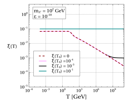
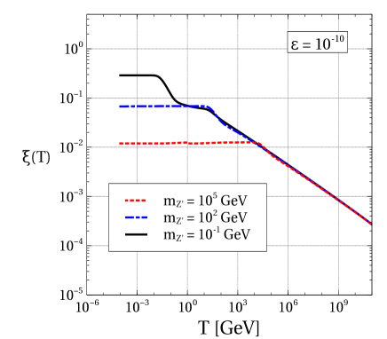
Considering all the processes mentioned above we solve Eq. 12 numerically and the numerical results are presented in the left panel of Fig. 2. We can see from the figure that for large value of $T$, $\xi(T)$ increases with the decrease in $T$ and it remains constant below $T\lesssim m_{Z^{\prime}}$ i.e. when all the energy injection processes stop. Since maximum production from inverse decay processes will occur at $T\sim m_{Z^{\prime}}$ therefore there is a small kink at $T\simeq m_{Z^{\prime}}$ in the figure for all values of $m_{Z^{\prime}}$.

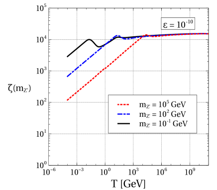
Since the collision term for all the production channels of $Z^{\prime}$ are proportional to $\epsilon^{2}$ therefore $\xi(T)$ should be proportional to $\sqrt{\epsilon}$. Thus to get a semi-analytic expression of $\xi(T)$, we parameterize $\xi(T)$ in the following manner.

$$\xi(T) = \zeta(m_{Z^{\prime}})\,\sqrt{\epsilon}\,T^{-1/4}\,\,,$$ (13)

where $\zeta(m_{Z^{\prime}})$ is a function of $m_{Z}^{\prime}$ and the choice of the temperature dependence is motivated by the discussion below Eq. 12. To determine the behaviour of $\zeta(m_{Z}^{\prime})$ we have calculated $\zeta(m_{Z^{\prime}})$ from our numerical results and plotted as a function of $T$ for three different values of $m_{Z^{\prime}}$ and $\epsilon=10^{-10}$ in the right panel of Fig. 2. From the figure we can see that $\zeta(m_{Z}^{\prime})$ does not depend on $m_{Z^{\prime}}$ and $T$ for $T\gtrsim\,10m_{Z^{\prime}}$ and in this region the value of $\zeta(m_{Z}^{\prime})\simeq 10^{4}$ Therefore we can write the semi-analytic form of $\xi(T)$ for $T>10\,m_{Z^{\prime}}$ as

$$\xi(T)\simeq 10^{4}\sqrt{\epsilon}\,T^{-1/4}\,\,.$$ (14)

Here, we would like to mention that, in our scenario, dark and visible sectors are not in thermal equilibrium and the value of $\xi$ depends on the portal coupling $\epsilon$.

Figure 2: Left panel: Variation of $\xi(T)$ as a function of $T$ for $m_{Z^{\prime}}=10^{-1}\,{\rm GeV}$ (solid black line), $m_{Z^{\prime}}=10^{2}\,{\rm GeV}$ (blue dashed-dot line), $m_{Z^{\prime}}=10^{5}\,{\rm GeV}$ (red dotted line). Right panel: Variation of $\zeta(m_{Z^{\prime}})$ as a function of $T$ and the values of $m_{Z^{\prime}}$ and color codes are same as left panel. In both the plots we have considered $\epsilon=10^{-10}$.

3.2 Non-adiabatic states of the dark sector

In this section we discuss various stages the of the dark sector during its cosmological evolution. Depending on the parameters of the dark sector, such as $m_{\chi}$, $m_{Z^{\prime}}$, $\alpha_{X}$ and also the portal coupling $\epsilon$, the states of the dark sector can be broadly classified into two parts and they are $i)$ equilibrium state and $ii)$ non-equilibrium state.

3.2.1 Equilibrium state

In case of non-adiabatic evolution, if the portal coupling is sufficiently high then the two sector equilibrate and they share a common temperature. This framework resembles with the initial idea of secluded sector DM in which the DM freezes out of a dark radiation bath which is in thermal equilibrium with the visible sector. Recently this scenario is named as “WIMP next door” Evans:2017kti .

In this work, we are interested in the scenario in which the dark sector is not in thermal equilibrium with the visible sector. To identify the parameter space in the $m_{\chi}-\epsilon$ plane for the thermally decoupled dark sector, first we identify the allowed parameter space in $m_{\chi}-\epsilon$ plane for the “WIMP next door” scenario. The disallowed region for the “WIMP next door” is the region of interest of our analysis.

For that we have assumed $\chi$, $Z^{\prime}$ are in thermal equilibrium with the SM bath. We have calculated total reaction rate ($\Gamma$) for the processes mentioned in section 3.1 and compared with the Hubble parameter $H(T)$. The ratio $\Gamma/H>1$ at $T\simeq m_{\chi}/20$ gives the allowed region for the “WIMP next door”. Note that we have considered the contribution of $Z^{\prime}$ in the Hubble parameter since it is assumed that $Z^{\prime}$ is in thermal equilibrium with the SM bath. A detailed discussion on the calculation of $\Gamma$ is given in Appendix C.

3.2.2 Non-equilibrium state

If the dark sector is not in thermal equilibrium then it may have its own temperature as we mentioned earlier. In this case depending on the model parameters such as $\epsilon$, $\alpha_{X}$, $m_{\chi}$ there are three possible stages of dark sector evolution and they are i) leak in, ii) freeze-in, iii) reannihilation.

Leak in:

The freeze-out of DM from the dark radiation bath during the production of dark radiation i.e. $Z^{\prime}$ from the SM bath is known as ‘Leak in dark matter’ (LIDM). In this scenario the final abundance of the DM depends on the ratio $\xi$ which is defined as $\xi=\dfrac{T^{\prime}}{T}$ and it is a function of $T$.

Nevertheless, there are clear differences between the dark sector freeze-out and leak in scenario. In the case of dark sector freeze-out it is assumed that the dark sector evolves adiabatically and the dark sector temperature $T^{\prime}=\xi T$, where $\xi$ is a constant quantity. In case of LIDM, the scenario is a little different. In this case the dark sector evolves non-adiabatically and DM freezes out during this non-adiabatic evolution.

To understand the LIDM mechanism quantitatively, let us discuss the abundance of DM in the leak in scenario. As discussed in section 3.1, the dark sector temperature during the energy injection epoch can be written as $T^{\prime}=\xi T$ where $\xi$ is a function of $T$. Now to get an approximate estimate of DM abundance we use sudden freeze-out condition $n_{\chi}(T^{\prime}_{f})\langle\sigma v\rangle\simeq H(T_{f})$ where $T_{f}(T^{\prime}_{f})$ is the temperature of the visible (dark) sector at the time of DM freeze-out, $\langle\sigma v\rangle$ is $2\to 2$ DM annihilation cross section, and $n_{\chi}(T^{\prime}_{f})$ is the DM number density at the time of DM freeze-out. Using the sudden freeze-out condition, the relic density of DM is given by

$$\Omega h^{2} \simeq 0.12\left(\dfrac{\xi}{10^{-5}}\right)\left(\dfrac{x_{f}^{\prime}}{10}\right)\left(\dfrac{7\times 10^{-15}\,{\rm GeV}^{-2}}{\langle\sigma v\rangle}\right)\left(\dfrac{\sqrt{g_{\rho}(T_{f})}}{10}\right)\left(\dfrac{100}{g_{*s}(T_{f})}\right)\,\,\,,$$ (15)

where $g_{\rho}(T)$ and $g_{*s}(T)$ are the relativistic degrees of freedom contributing to the energy density and the entropy density of the SM respectively and $x^{\prime}_{f}=m_{\chi}/T^{\prime}_{f}$.

Now we can see from Eq. 15 that the required cross section to get correct relic abundance is much smaller than the required cross section ($\approx$ $10^{-8}\,{\rm GeV}^{-2}$) for standard WIMP scenario. Thus LIDM scenario naturally indicates that the mass of the DM should be heavy and the relevant discussion is given below.

The upper limit of the DM mass can be set from the S-matrix unitarity Griest:1989wd in the LIDM scenario. The s-wave term of the thermally averaged DM annihilation cross section is given by Griest:1989wd

$$\langle\sigma v\rangle_{\rm Max} \simeq \dfrac{4\pi}{m_{\chi}^{2}}\sqrt{\dfrac{x^{\prime}_{f}}{\pi}}\,\,.$$ (16)

Thus using Eq. 16 in Eq. 15 we get the upper bound of the DM mass which is given by

$$m_{\chi}\lesssim\dfrac{127\,\rm TeV}{\sqrt{\xi}}\,\,.$$ (17)

Thus $\xi$ plays an important role in determining the upper limit of $m_{\chi}$ and for $\xi$ to be much smaller than 1, the upper limit of the DM mass is much larger in comparison to the standard WIMP scenario. For example if we consider $\xi=10^{-5}$ and $\chi$ to be dirac fermion then $m_{\chi}\lesssim 40\,{\rm PeV}$ whereas for standard WIMP scenario the upper limit of the DM mass is $m_{\chi}\lesssim 127\,\rm TeV$. In deriving these numbers we have used the sudden freeze-out approximation and $x^{\prime}_{f}\simeq 10$.

Freeze-in:

Feebly interacting massive particle (FIMP) is a well studied scenario and it is motivated by the null results of (in)direct searches. In this scenario the DM is produced out of equilibrium from the SM bath and the production stops at $T\sim{\rm Max}[m_{\chi},m_{\rm SM}]$ where $m_{\rm SM}$ is the mass of the parent particles. Therefore the abundance of the DM is set by out of equilibrium production of DM from SM bath. Since the DM is out of equilibrium with the SM bath therefore its coupling with the SM is very weak ($\sim 10^{-10}$) and it can easily explain the null results of the experimental searches.

In our model, the DM particle $\chi$ is in thermal equilibrium with the dark radiation bath and it follows the equilibrium number density. After decoupling from the dark radiation bath, the abundance of $\chi$ can be increased due to the presence of the DM production channel $\bar{f}f\to\bar{\chi}\chi$ where ($f=\mu,\tau,\nu_{\mu},\nu_{\tau}$). Since we have assumed $\epsilon<<1$ therefore the abundance of $\chi$ freezes at $T\sim{\rm Max}[m_{f},m_{\chi}]$ provided $\alpha_{X}$ is not sufficiently high. Thus in our scenario it is possible that the final DM abundance is set by the freeze-in mechanism.

Reannihilation:

If the coupling between the dark sector particles are sufficiently high then there is a possibility that the excess DM produced via freeze-in can reannihilate into the dark sector particles. In this situation if the rate of production of DM via freeze-in and the rate of depletion via reannihilation are equal then it follows a quasi static equilibrium and finally it freezes-out when the DM decouples from the quasi-static equilibrium Cheung:2010gj ; Chu:2011be . This phenomenon is known as reannihilation. In our model, for larger values of $\alpha_{X}$ compared to the freeze-in scenario, it is possible that the DM produced via freeze-in, reannihilate into the dark vector boson $Z^{\prime}$. Therefore in this case final abundance of the DM is set by the reannihilation mechanism.

3.3 Boltzmann Equation

In this section we formulate the Boltzmann equation for the evolution of the DM number density. As discussed in section 6 that the dark sector temperature can be expressed as a function of $T$ and $\epsilon$. Therefore we can obtain the final relic abundance of DM by solving the Boltzmann equation considering a different dark sector temperature ($T^{\prime}$). The Boltzmann equation for the number density of $\chi$ is given by

$$\dfrac{dn_{\chi_{\rm tot}}}{dt}+3Hn_{\chi_{\rm tot}} = \dfrac{1}{2}\left[\langle\sigma v\rangle^{T^{\prime}}_{\bar{\chi}\chi\to Z^{\prime}Z^{\prime}}\left(n_{\chi_{\rm eq_{\rm tot}}}(T^{\prime})^{2}-n_{\chi_{\rm tot}}^{2}\right)\right]$$ (18)

$$+ 2\sum_{f}\langle\sigma v\rangle^{T}_{\bar{f}{f}\to\bar{\chi}{\chi}}n_{f_{{\rm eq}}}^{2}(T)$$

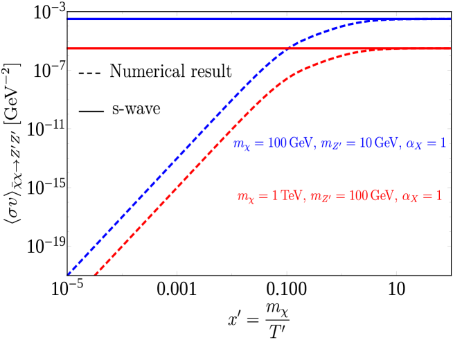
The first term on the left hand side of Eq. 18 denotes the change in DM number density ($n_{\chi_{\rm tot}}=n_{\chi}+n_{\bar{\chi}}$) whereas the second term implies the dilution of $n_{\chi_{\rm tot}}$ due to expansion of the Universe. The first term on the right hand side of Eq. 18 denotes the DM interaction with the $Z^{\prime}$ bath and $\langle\sigma v\rangle^{T^{\prime}}_{\bar{\chi}{\chi}\to Z^{\prime}Z^{\prime}}$ is thermally averaged cross section of $\bar{\chi}{\chi}\to Z^{\prime}Z^{\prime}$ calculated at temperature $T^{\prime}$. The s-wave term of the thermal average of the $\bar{\chi}{\chi}\to Z^{\prime}Z^{\prime}$ cross section is given by

$$\langle\sigma v\rangle_{\bar{\chi}{\chi}\to Z^{\prime}Z^{\prime}} \simeq \dfrac{4\pi\alpha_{X}^{2}}{m_{\chi}^{2}}\dfrac{m_{\chi}\left(m_{\chi}^{2}-m_{Z^{\prime}}^{2}\right)^{3/2}}{\left(2m_{\chi}^{2}-m_{Z^{\prime}}^{2}\right)^{2}}\,\,.$$ (19)

In Fig. 3, we have plotted the variation of numerically calculated $\langle\sigma v\rangle_{\bar{\chi}{\chi}\to Z^{\prime}Z^{\prime}}$ as a function of $x^{\prime}=m_{\chi}/T^{\prime}$ for two benchmark values of $m_{\chi}$, $m_{Z^{\prime}}$, and $\alpha_{X}$ along with the s-wave term of $\langle\sigma v\rangle_{\bar{\chi}{\chi}\to Z^{\prime}Z^{\prime}}$. From the plot it is clear that the s-wave term coincides with the numerically evaluated thermal average for $x^{\prime}\gtrsim 1$. Since the DM freezes out at $x^{\prime}\sim 10$, we can safely use the s-wave annihilation cross section, given in Eq. 19.

Figure 3: Variation of $\langle\sigma v\rangle_{\bar{\chi}{\chi}\to Z^{\prime}Z^{\prime}}$ as a function of $x^{\prime}$ for two benchmark values of $m_{\chi}$, $m_{Z^{\prime}}$, and $\alpha_{X}$. The dashed and the solid lines denote the numerical result and s-wave term of $\langle\sigma v\rangle_{\bar{\chi}{\chi}\to Z^{\prime}Z^{\prime}}$ respectively. The blue lines are plotted for $m_{\chi}=100\,{\rm GeV}$, $m_{Z^{\prime}}=10\,{\rm GeV}$, and $\alpha_{X}=1$ whereas for the red lines we consider $m_{\chi}=1\,{\rm TeV}$, $m_{Z^{\prime}}=100\,{\rm GeV}$, and $\alpha_{X}=1$.

The second term on the right hand side of Eq. 18 is responsible for the production of DM from SM bath and $\langle\sigma v\rangle^{T}_{\bar{f}{f}\to\bar{\chi}\chi}$ is the thermally averaged cross section of $\bar{f}{f}\to\bar{\chi}{\chi}$ where $f=\{\mu,\tau,\nu_{\mu},\nu_{\tau}\}$ and it is calculated at temperature $T$. Since the DM is not in thermal contact with the SM bath therefore we have neglected the production of SM particles from DM annihilation. The thermally averaged cross section of $\bar{f}{f}\to\bar{\chi}{\chi}$ is defined as follows.

$$\langle\sigma v\rangle_{\bar{f}{f}\to\bar{\chi}{\chi}} = \dfrac{1}{n_{f_{\rm eq}}^{2}(T)}\dfrac{g_{f}^{2}T}{2(2\pi)^{4}}\int_{{\rm Max}\left[4m_{\chi}^{2},4m_{f}^{2}\right]}^{\infty}\sigma_{\bar{f}{f}\to\bar{\chi}{\chi}}\sqrt{\hat{s}}\left(\hat{s}-4m_{f}^{2}\right)K_{1}\left(\dfrac{\sqrt{\hat{s}}}{T}\right)\,d\hat{s}\,\,.$$ (20)

Here $n_{f_{\rm eq}}(T)$ is the equilibrium number density of the annihilating fermion $f$ at temperature $T$, $g_{f}$ is the internal degrees of freedom of $f$, and $\hat{s}$ is the Mandelstam variable. In Eq. 20, $K_{1}(\sqrt{\hat{s}}/T)$ is the modified Bessel function of second kind and order one. The analytical form of the annihilation cross sections of $\bar{f}f\to\bar{\chi}{\chi}$ are given by

$$\sigma_{\bar{f}{f}\to\bar{\chi}{\chi}} = \dfrac{\alpha_{X}\epsilon^{2}}{3\hat{s}}\sqrt{\dfrac{\hat{s}-4m_{\chi}^{2}}{\hat{s}-4m_{f}^{2}}}\dfrac{(\hat{s}+2m_{f}^{2})(\hat{s}+2m_{\chi}^{2})}{(\hat{s}-m_{Z^{\prime}}^{2})^{2}}~{}~{}~{}~{}~{}\text{for }f=\mu,\,\tau\,\,,$$ (21)

$$\sigma_{\bar{\nu}_{i}{\nu_{i}}\to\bar{\chi}\chi} = \dfrac{\alpha_{X}\epsilon^{2}}{6}\sqrt{\dfrac{\hat{s}-4m_{\chi}^{2}}{\hat{s}}}\dfrac{\hat{s}+2m_{\chi}^{2}}{(\hat{s}-m_{Z^{\prime}}^{2})^{2}}~{}~{}~{}~{}\text{for }\nu_{i}=\nu_{\mu},\,\nu_{\tau}\,\,.$$ (22)

In Eq. 18, $n_{{\chi_{\rm eq}}_{\rm tot}}(T^{\prime})$ and $n_{{\chi_{\rm eq}}_{\rm tot}}(T)$ are the equilibrium number densities of $\chi+\bar{\chi}$ calculated at temperatures $T^{\prime}$ and $T$ respectively. Let us note that the 1/2 (2) factor in the first (second) term on the right hand side of this equation arises because of the fact that the DM candidate is a Dirac fermion.

To solve Eq. 18 we define the comoving number density $Y_{\chi_{\rm tot}}$ as $Y_{\chi_{\rm tot}}=n_{\chi_{\rm tot}}/s(T)$ where $s(T)=\dfrac{2\pi^{2}}{45}g_{*s}(T)T^{3}$ is the entropy density of the SM bath and $g_{*s}(T)$ is the relativistic degrees of freedom contributing to the entropy density of the SM bath. Now defining $x=m_{\chi}/T$ and using the conservation of entropy of the SM bath (approximately), we can arrive at the following equation.

$$\dfrac{dY_{\chi_{\rm tot}}}{dx} = \dfrac{h_{\rm eff}(x)}{2}\dfrac{s(x)}{xH(x)}\langle\sigma v\rangle^{T^{\prime}}_{\bar{\chi}\chi\to Z^{\prime}Z^{\prime}}\left(Y_{\chi_{{\rm eq}_{\rm tot}}}(T^{\prime},T)^{2}-Y_{\chi_{\rm tot}}^{2}\right)$$ (23)

$$+ \dfrac{2\,h_{\rm eff}(x)s(x)}{xH(x)}\sum_{f}\langle\sigma v\rangle^{T}_{\bar{f}{f}\to\bar{\chi}\chi}Y_{f_{{\rm eq}}}^{2}(T)\,\,,$$

where $Y_{\chi_{{\rm eq}_{\rm tot}}}(T,T^{\prime})=\dfrac{n_{\chi_{{\rm eq}_{\rm tot}}}(T^{\prime})}{s(T)}$, $Y_{f_{\rm eq}}(T)=\dfrac{n_{f_{\rm eq}}(T)}{s(T)}$ and $h_{\rm eff}(x)=\left(1-\dfrac{1}{3}\dfrac{d\ln g_{*s}(x)}{d\ln x}\right)$.

Now in the right hand side of Eq. 23, if the first term is dominant over the second one i.e. if the freeze-in term is negligible then comoving number density of DM is only governed by the annihilation cross section of $\bar{\chi}\chi\to Z^{\prime}Z^{\prime}$ and also the dark sector temperature $T^{\prime}$ which depends on $\epsilon$ and $T$. Thus in this case DM freezes out at $x^{\prime}_{\rm FO}\sim 10$ and this is known as the “LIDM” scenario. However if the freeze-in term is not negligible then in that case after decoupling of the DM, its comoving number density can be increased due to the DM production from SM bath and the production freezes at $x_{\rm FI}\sim 1$. In this case the final relic density of DM does not depend on the first term of Eq. 23 and it is known as “freeze-in”. Thus the final relic density is independent of the $\bar{\chi}\chi\to Z^{\prime}Z^{\prime}$ annihilation cross section. In case of reannihilation, after the departure from the equilibrium number density, the DM produced from the SM bath due to the presence of the freeze-in term can reannihilate into $Z^{\prime}$ if the dark sector coupling is sufficiently large. Therefore in this case both the term on the right hand side of Eq. 23 contribute to the final relic abundance.

Depending on the time ordering of $x_{\rm FO}$ (corresponding to $x^{\prime}_{\rm FO}\sim 10$) and $x_{\rm FI}$ the LIDM scenario can be classified into two parts:

i) If $x_{\rm FO}<x_{\rm FI}$ then freeze-in term is triggered after the DM freezes out and in this case the final relic abundance slightly depends on the freeze-in term. This is known as “early-LIDM”,

ii) If $x_{\rm FO}>x_{\rm FI}$ then freeze-out occurs after the production of DM stops. In that case since DM follows the equilibrium number density during the production via freeze-in therefore the produced DM can rapidly thermalise with the $Z^{\prime}$ bath. Thus the final relic abundance is independent of the freeze-in term. This is known as “Late LIDM”.

In the next section we show our numerical results for each of the above mentioned scenarios and also the allowed parameter space for LIDM, freeze-in, and reannhilation.

4 Numerical results for Dark Matter relic density

In this section we discuss the numerical results of our analysis. We have solved the Boltzmann equation for the total number density of the DM candidate by considering the fact that the dark sector evolves non-adiabatically and its temperature evolution is given by the semi-analytic result in Eq. 14. Using the solution of the Boltzmann equation we can compute the final relic abundance of $\chi$ from the following relation.

$$\Omega h^{2}=2.755\times 10^{8}\left(\dfrac{m_{\chi}}{1\,\rm GeV}\right)Y^{0}_{\chi_{\rm tot}}\,\,,$$ (24)

where $Y^{0}_{\chi_{\rm tot}}$ is the present value of the DM comoving number density. The initial conditions for solving the Boltzmann equation are $x=x_{in}=10^{-4}$ and $Y_{\chi_{\rm tot}}=Y_{\chi_{{\rm eq}_{\rm tot}}}(T_{in},T^{\prime}_{in})$ where $T_{in}=m_{\chi}/x_{in}$ and $T^{\prime}_{in}=\xi(T_{in})T_{in}$. In choosing the initial condition we have assumed the DM follows the equilibrium distribution at $x=x_{in}$ and the validity of this assumption will be discussed in Appendix D. Let us note that in our numerical analysis we choose $r=m_{Z^{\prime}}/m_{\chi}=0.1$ for the calculation of the DM relic density and parameter spaces allowed from the relic density constraint remain unaltered for other choices of $r$. The only required condition is at the time of DM freeze-out $Z^{\prime}$ should behave as radiation and only in that case we can write its energy density proportional to ${T^{\prime}}^{4}$. Therefore at the time of DM freeze-out $T^{\prime}_{f}\gtrsim m_{Z^{\prime}}$ which implies $r^{-1}\gtrsim 10$ (considering $x^{\prime}_{f}\sim 10$). We would also like to mention that in our numerical analysis we have used Eq. 14 in the expression of $Y_{\chi_{{\rm eq}_{\rm tot}}}$. Since this relation is valid for $T\gtrsim 10m_{Z^{\prime}}$, we can write this relation as $r^{-1}\gtrsim 10\,x$ where we have used $T=m_{\chi}/x$. Since DM freezes-out as $x<1$ therefore this condition is satisfied for $r\leq 10^{-1}$. Thus we can safely use Eq. 14 for the expression of $T^{\prime}$.

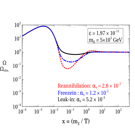
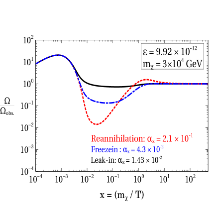
In Fig. 4 we show the evolution of the relative abundance of the DM (defined as the ratio between the DM abundance evaluated from Eq. 24 to the observed value of the DM relic density ($\Omega h^{2}_{\rm Obs.}\simeq 0.12$)) as a function $x$ for two benchmark values of the model parameters. In each of the plots we fix the value of $m_{\chi}$ and $\epsilon$ and vary $\alpha_{X}$ to get the final relic abundance. Let us consider the left panel of Fig. 4. In this figure, for $\alpha_{X}=5.2\times 10^{-3}$, the DM decouples at $x\sim 10^{-2}$ from dark radiation bath and its abundance increases slightly due to the presence of the freeze-in term in the Boltzmann equation. The increase in the DM abundance stops at $x\sim 2$ and after that it remain constant. This is known as the ‘early-LIDM’ as discussed earlier and it is denoted by the solid black line. Now if we increase $\alpha_{X}$, the results of the increase are two fold. Firstly with the increase in $\alpha_{X}$ the DM interacts with the radiation bath more strongly and there will be a delay in the decoupling of the DM. Secondly for large values of $\alpha_{X}$ the freeze-in term plays a crucial role since it is proportional to $\alpha_{X}$ and depending on the values of $\alpha_{X}$ the final DM abundance is either set by freeze-in mechanism or reannihilation. From the figure one can see that for $\alpha_{X}=1.2\times 10^{-2}$ the final abundance of the DM is set only by the production of the DM from SM bath and the production freezes at $x\sim 2$. Thus in this case the first term in the right hand side of Eq. 23 does not play any significant role. This is known as Freeze-in mechanism which is depicted by blue dashed-dot line. In contrast to that for $\alpha_{X}=2.8\times 10^{-2}$ the production of DM from the SM bath is sufficient to rethermalise the DM with $Z^{\prime}$. Therefore both the term in the right hand side of Eq. 23 determine the final relic abundance and reannihilation occurs. The red dotted line indicates the reannihilation mechanism of DM. In the right panel of Fig. 4 we show all of the three mechanisms discussed earlier with the same color codes but with different choice of the parameters. Let us note that for both the plots we choose $m_{Z^{\prime}}=0.1m_{\chi}$ and the results shown in Fig. 4 are independent of this choice as long as $m_{Z^{\prime}}\leq 0.1m_{\chi}$.

Figure 4: Left panel: The variation of relative abundance of DM as a function of $x$ for $m_{\chi}=5\times 10^{3}\,{\rm GeV}$, $\epsilon=1.97\times 10^{-11}$ and for three difference choice of $\alpha_{X}$. The three different mechanisms i.e. early leak in ($\alpha_{X}=5.2\times 10^{-3}$), freeze-in ($\alpha_{X}=1.2\times 10^{-2}$), and reannihilation ($\alpha_{X}=2.8\times 10^{-2}$) are depicted by solid black, blue dashed-dot, and red dotted lines respectively. Right panel: The variation of relative abundance of DM as a function of $x$ for $m_{\chi}=3\times 10^{4}\,{\rm GeV}$, $\epsilon=9.92\times 10^{-12}$ and for three difference choice of $\alpha_{X}$. Here, early leak in ($\alpha_{X}=1.43\times 10^{-2}$), freeze-in ($\alpha_{X}=4.3\times 10^{-2}$), and reannihilation ($\alpha_{X}=2.1\times 10^{-1}$) are depicted by solid black, blue dashed-dot, and red dotted lines respectively. In both the panel we have considered $m_{Z^{\prime}}=0.1m_{\chi}$.

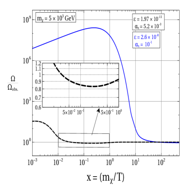
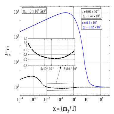
As we discussed earlier, depending on the time ordering of $x_{\rm FO}$ and $x_{\rm FI}$ LIDM scenario can be classified into early-LIDM and late-LIDM. In Fig. 5 we show the evolution of the relative DM abundance as a function of $x$ for both the LIDM scenarios. Since the equilibrium comoving number density of the DM increases with the increase in $\epsilon$ therefore for large values of $\epsilon$ we need large annihilation cross section to get the correct relic abundance and thus the DM is in thermal contact with the dark radiation bath for longer time. In this case the production of DM from SM bath does not play any significant role if the DM is in thermal contact with dark radiation bath. This is because the DM produced from SM bath will rapidly annihilate into $Z^{\prime}$. Thus the comoving number density of DM remains unaltered despite the fact that the freeze-in term of the Boltzmann equation is not negligible. This scenario is known as ‘late-LIDM’ and blue solid line of each panel of this figure indicates the DM coving number density for late-LIDM scenario.

However the situation is different for small values of $\epsilon$ and $\alpha_{X}$. In this case the DM decouples much earlier compared to late-LIDM scenario and the production of DM from the SM bath occurs after the decoupling of DM. Therefore the final abundance of the DM increases slightly at $x\sim 2$. This phenomenon is called as ‘early-LIDM’. In both the panel the black dashed lines depict the early-LIDM scenario.

Figure 5: Left panel: Evolution of the relative DM abundance as a function of $x$ in case of late and early LIDM for $m_{\chi}=5\times 10^{3}\,{\rm GeV}$. The late-LIDM mechanism is shown by the blue solid line and the values of $\epsilon$ and $\alpha_{X}$ are $2.6\times 10^{-8}$ and $10^{-1}$ respectively. The black dashed line depicts the early-LIDM scenario for $\epsilon=1.97\times 10^{-11}$ and $\alpha_{X}=5.2\times 10^{-3}$. Right panel: DM relative abundance as a function of $x$ for $m_{\chi}=3\times 10^{4}\,{\rm GeV}$. The color codes are same as left panel but the corresponding values of $\epsilon$ and $\alpha_{X}$ are different (for late-LIDM $\epsilon=6.4\times 10^{-8}$, $\alpha_{X}=6.8\times 10^{-1}$ (blue solid line), and for early-LIDM $\epsilon=9.92\times 10^{-12}$, $\alpha_{X}=1.45\times 10^{-2}$ (black dashed line)). In both the panel the value of $m_{Z^{\prime}}=0.1m_{\chi}$.

Finally in Fig. 6 we show the allowed parameter space in $m_{\chi}-\epsilon$ plane from relic density along with other experimental constraints. In this plot we show the contours of $\alpha_{X}=1,10^{-2},10^{-4}$ with black dashed lines. Because the dark sector temperature increases with the increase in $\epsilon$, we need higher values of annihilation cross section to satisfy the correct relic abundance. This implies that for constant $\alpha_{X}$, $m_{\chi}$ should decrease as we increase $\epsilon$. One can clearly see this pattern for each contour of constant $\alpha_{X}$. We can see for a fixed value of $\epsilon$, $m_{\chi}$ increases with the increase in $\alpha_{X}$. This behaviour can be understood as follows. For a fixed value of $\epsilon$, annihilation cross section increases due to the increase in $\alpha_{X}$ and this enhancement in the cross section should be counterbalanced by the increase in $m_{\chi}$ to satisfy the correct relic density. However for lower values of $\epsilon$ i.e. $\epsilon\lesssim 10^{-11}$ all the contours of constant $\alpha_{X}$ coincide and in that case for fixed value of $m_{\chi}$ and $\epsilon$ one can obtain many relic density satisfied points for different values of $\alpha_{X}$. Thus in this region, for a fixed value of $m_{\chi}$ and $\epsilon$, the mechanisms of getting correct relic abundance are different and they depend on the values of $\alpha_{X}$. The purple and light red region in this figure denote the relic density satisfied region via reannihilation and leak-in mechanisms respectively. The red patch in the parameter space denotes the region at which leak-in, freeze-in, and reannihilation occurs. In Fig. 4 we showed the leak-in, freeze-in, and reannihilation for two fixed values of $m_{\chi}$ and $\epsilon$ and these two points are shown with yellow marked points in Fig. 6.

As mentioned earlier the dark sector is not in thermal equilibrium with the SM bath therefore we have identified the parameter space for this scenario according to the discussion in section 3.2.1. The green region of Fig. 6 indicates the allowed region for the WIMP next door scenario. The parametric dependence of the $\Gamma/H$ ratio is given by $\epsilon^{2}/m_{\chi}$. Thus in this region $\epsilon$ increases with the increase in $m_{\chi}$ and this dependence can be seen clearly from the figure.

Figure 6: Allowed parameter space in $m_{\chi}-\epsilon$ plane where the contours of $\alpha_{X}=10^{-4},10^{-2},1$ are shown with the dashed lines. The points mentioned in Fig. 4 are shown with yellow marked points at which leak-in, freeze-in, and reannihilation occur. Parameter space for LIDM is shown with light red color whereas purple region represents the parameter space for reannihilation. The small red patch corresponds to the region where all of the three non-equilibrium stages namely leak-in, freeze-in, and reannihilation are possible. The green region is the parameter space for WIMP next door scenario and the region in which $\alpha_{X}>4\pi$ is shown by the brown color. Cyan region shows the parameter space for not internally thermalised dark sector (considering $m_{Z^{\prime}}/m_{\chi}=10^{-6}$) whereas in the orange region the number density of the DM is not sufficient to produce correct relic abundance. The constraint from self interacting dark matter (SIDM) is shown by the pink color for two values of $r$ ($r=10^{-2}$ (dotted line), $r=10^{-3}$ (dashed line)). They grey and blue region show the direct detection and CMB constraint for $r=10^{-3}$ and $r=10^{-1}$ respectively.

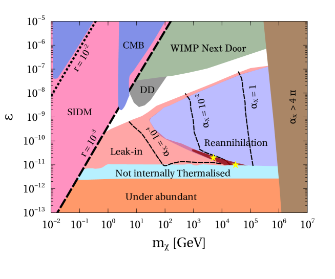
The equilibrium number density of the DM depends on the dark sector temperature $T^{\prime}$ which is proportional to $\epsilon^{1/2}$. Thus equilibrium number density decreases with the decrease in $\epsilon$. This means there will be a minimum value of $\epsilon$ below which it is not possible to get the correct relic abundance. The orange region of Fig. 6 shows the minimum values of $\epsilon$ below which we cannot obtain correct relic abundance. This region has been obtained from the condition $Y_{\chi_{{\rm eq}_{\rm tot}}}|_{\rm max}(T^{\prime}_{0})\leq\left(0.12/2.755\times 10^{8}\right)(1\,{\rm GeV}/m_{\chi})$ where $Y_{\chi_{{\rm eq}_{\rm tot}}}|_{\rm max}(T^{\prime}_{0})$ is the maximum value of the comoving number density of DM and $T^{\prime}_{0}=2m_{\chi}/5$ is the value of the dark sector temperature at which maximum occurs Evans:2019vxr .

The brown region of the figure represents that the required values of $\alpha_{X}$ for correct relic density belongs to the non-perturbative regime of $\alpha_{X}$ i.e. in this region of parameter space $\alpha_{X}>4\pi$.

We have also shown the constraints from internal thermalisation of the dark sector by cyan region and the relevant discussion is given in Appendix D. There are other constraints such as self interactions of dark matter (pink region), direct detection (DD) (grey region), CMB (blue region). In deriving these constraints we express $\alpha_{X}$ in terms of $\epsilon$ and $m_{\chi}$ (this can be done by using Eq. 14, Eq. 15 and Eq. 19) to identify the parameter space only for LIDM. In section 5 we will discuss these constraints in detail and we will also discuss the allowed parameter space in $m_{\chi}-\alpha_{X}$ plane by considering $\alpha_{X}$ and $\epsilon$ as independent parameters.

5 Detection prospect of the Dark Matter

The parameter space of our model can be constrained from various astrophysical and laboratory experiments. In this section we will discuss the constraints on the model parameters such as $\epsilon$, $m_{\chi}$, $m_{Z^{\prime}}$, and $\alpha_{X}$.

5.1 Direct Detection

In our model DM interacts with SM particles (namely, second and third generation leptons) through the kinetic mixing of $Z^{\prime}$ and $Z_{\mu\tau}$. Although there is no tree level interaction of DM with quarks but still interaction can happen through the radiatively generated $Z-Z^{\prime}$ and $\gamma-Z^{\prime}$ kinetic mixing. Therefore we have calculated spin independent DM-nucleon scattering cross section to study the direct detection constraint and the scattering cross section in the low momentum transfer limit is given by

$$\sigma^{\rm SI}_{\chi n} = \frac{4\alpha_{X}\mu_{\chi n}^{2}}{m_{Z^{\prime}}^{4}}|\Pi(0)|^{2}\left[\frac{Z}{A}f_{p}+\left(1-\frac{Z}{A}\right)f_{n}\right]^{2}\,\,,$$ (25)

where $\mu_{\chi n}=\frac{m_{n}m_{\chi}}{m_{n}+m_{\chi}}$ is the reduced mass of the DM-nucleon system and $m_{n}$ is the mass of a nucleon. $A(Z)$ is the mass (atomic) number of target nucleus. $f_{p}$ and $f_{n}$ are defined as follows Berlin:2014tja : $f_{p}=2Q_{u}+Q_{d}$ and $f_{n}=Q_{u}+2Q_{d}$, where $Q_{u}\left(Q_{d}\right)$ is electromagnetic charge of up (down) quark. The radiatively generated kinetic mixing between $Z^{\prime}$ and $\gamma$ at one loop level is given by Araki:2017wyg ; Banerjee:2018mnw

$$i\Pi(q^{2})=-\frac{ie\epsilon}{2\pi^{2}}\int_{0}^{1}x(1-x)\ln\left(\dfrac{m_{\mu}^{2}-q^{2}x(1-x)}{m_{\tau}^{2}-q^{2}x(1-x)}\right)dx\,\,\,,$$ (26)

where $e=\sqrt{4\pi\alpha_{\rm em}}$ is the charge of the electron and $\alpha_{\rm em}$ is the fine-structure constant. In the limit $q^{2}\to 0$ Eq. 26 takes the following form.

$$i\Pi(0)=-\frac{ie\epsilon}{12\pi^{2}}\ln\left(\dfrac{m_{\mu}^{2}}{m_{\tau}^{2}}\right)\,\,.$$ (27)

Moreover we have also considered the DM-electron scattering for low mass DM and the corresponding scattering cross section in the low momentum transfer limit is given by

$$\sigma_{e} = \dfrac{16\pi\alpha_{X}\alpha_{\rm em}\,\mu_{\chi e}^{2}}{m_{Z^{\prime}}^{4}}|\Pi(0)|^{2}\,\,,$$ (28)

where $\mu_{\chi e}=\frac{m_{\chi}m_{e}}{m_{\chi}+m_{e}}$ is the reduced mass of the DM-electron system.

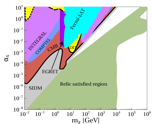
Now we have compared the spin independent direct detection cross sections given in Eq. 25 and Eq. 28 with the current bounds from the direct detection experiments XENON1T XENON:2018voc , CRESST-III CRESST:2019jnq , and XENON10T XENON10:2011prx ; Essig:2017kqs . The excluded region of the parameter space in $m_{\chi}-\alpha_{X}$ plane from direct detection constraint for $\epsilon=10^{-9}$ and $r=m_{Z^{\prime}}/m_{\chi}=10^{-3}$ is shown in Fig. 7 by yellow color and this bounds will be more stringent for smaller values of $r$.

5.2 CMB constraint

Production of SM charged particles from the annihilation of DM can alter the ionisation history of Hydrogen at the time of CMB. The amount of energy injected per annihilation within the volume $\Delta V$ and time $\Delta t$ is given by

$$\Delta E=2m_{\chi}\left(\dfrac{n_{\chi}}{2}\right)^{2}_{\rm CMB}\langle\sigma v\rangle_{\bar{\chi}{\chi}\to\rm SM}\Delta V\Delta t\,\,\,,$$ (29)

where $n_{\chi}$ is the number density of DM at the time of CMB and $\langle\sigma v\rangle_{\bar{\chi}{\chi}\to\rm SM}$ is the annihilation cross section of DM into SM particles. Now using the conservation of total number of DM we can write the expression of the amount of deposited energy as follows.

$$\dfrac{dE}{dVdt}=(1+z)^{6}\rho_{c}^{2}\,\Omega h^{2}\,\mathcal{P}_{\rm ann}\,\,\,,$$ (30)

where $\mathcal{P}_{\rm ann}=\dfrac{f_{\rm eff}(m_{\chi})}{2}\dfrac{\langle\sigma v\rangle_{\bar{\chi}{\chi}\to SM}}{m_{\chi}}$, $z$ is the redshift parameter, and $f_{\rm eff}$ is the redshift independent efficiency factor Slatyer:2015jla . For the $s$-wave DM annihilation the upper limit of $\mathcal{P}_{\rm ann}$ is $4.1\times 10^{-28}\rm\,cm^{3}\,s^{-1}\,GeV^{-1}$ Planck:2015fie . Therefore using the expression of $\mathcal{P}_{\rm ann}$ we can write

$$\sum_{\rm SM}f^{\rm SM}_{\rm eff}(m_{\chi})\dfrac{\langle\sigma v\rangle_{\bar{\chi}\chi\to Z^{\prime}Z^{\prime}}{\rm Br}(Z^{\prime}\to\rm SM)}{m_{\chi}}<8.2\times 10^{-28}\rm\,cm^{3}\,s^{-1}\,GeV^{-1}\,\,.$$ (31)

In deriving the CMB bound we have used Eq. 31 and the corresponding excluded region for $r=10^{-1}$ is shown in Fig. 7 with red color. The CMB bound for $r=10^{-1}$ is maximum and it relaxes with the decrease in $r$ because of the reduction of the branching ratios of $Z^{\prime}$ into SM particles.

5.3 Dark matter self interaction

From the bullet cluster observations, the upper limit of the self-interaction cross section of DM is bounded as $\sigma_{T}/m_{\chi}<1.25\,{\rm cm}^{2}\,{\rm g}^{-1}$ Randall:2008ppe where $\sigma_{T}$ is the momentum transfer cross section of DM-DM scattering process. To derive the allowed parameter space from the bullet cluster observation, we have calculated the momentum transfer cross sections of $\bar{\chi}\chi\rightarrow\bar{\chi}\chi$, $\chi\chi\rightarrow\chi\chi$, and $\bar{\chi}\bar{\chi}\rightarrow\bar{\chi}\bar{\chi}$ and defined an effective cross section as Choi:2016tkj

$$\sigma_{T}=\dfrac{1}{4}\left(\sigma^{T}_{\bar{\chi}\chi\rightarrow\bar{\chi}\chi}+\sigma^{T}_{\bar{\chi}\bar{\chi}\rightarrow\bar{\chi}\bar{\chi}}+\sigma^{T}_{\chi\chi\rightarrow\chi\chi}\right)\,\,,$$ (32)

where $1/4$ factor is due to the fact that there is no asymmetry between particle and anti-particle, therefore both of them contribute equally to the relic density.

The bounds from self-interacting DM has been shown in Fig. 7 by the grey region for $r=10^{-3}$ and this bound will be stronger as we decrease $r$.

Figure 7: Parameter space in $m_{\chi}-\alpha_{X}$ plane. The green region is the relic density satisfied region whereas the grey region is excluded from the bullet cluster observation for $r=10^{-3}$. The red region is excluded from the observations of CMB for $r=10^{-1}$. The yellow region outlined with solid, dashed, and dotted line represent the direct detection constraint from XENON1T, CRESST-III, and XENON10T for $\epsilon=10^{-9}$, and $r=10^{-3}$. The bounds arising from the measurement of diffuse $\gamma$-ray background flux (discussed below) by EGRET, INTEGRAL, COMPTEL, and Fermi-LAT are shown by violet, purple, blue, and cyan regions respectively for $r=10^{-1}$.

5.4 $\gamma$-ray signal from DM annihilation

In our framework we will study the prospect of detecting $\gamma$ ray signal from DM annihilation via one step cascade process. In this process, DM annihilates into a pair of $Z^{\prime}$ and one of this $Z^{\prime}$ can decay into a pair of SM charged particles. The differential photon flux originating from this type of one step cascade process is given by

$$\dfrac{d\Phi}{dE_{\gamma}\Delta\Omega} = \dfrac{\langle\sigma v\rangle_{\bar{\chi}\chi\to Z^{\prime}Z^{\prime}}}{16\pi m_{\chi}^{2}}\rho_{\odot}^{2}R_{\odot}\bar{J}_{\rm ann}\sum_{f}{\rm Br}(Z^{\prime}\to\bar{f}f)\dfrac{dN^{f}_{\gamma}}{dE_{\gamma}}\,\,,$$ (33)

where $\dfrac{dN^{f}_{\gamma}}{dE_{\gamma}}$ is the photon spectrum for the DM annihilation into $\bar{f}f$ pair where $f$ is a SM charged fermion and the spectrum is calculated in the centre of mass (CoM) frame of the DM annihilation. $\langle\sigma v\rangle_{\bar{\chi}\chi\to Z^{\prime}Z^{\prime}}$ is the annihilation cross section of DM into a pair of $Z^{\prime}$ and the s-wave term of the annihilation cross section is given in Eq. 19. In Eq. 33, ${\rm Br}(Z^{\prime}\to\bar{f}f)$ is the branching ratio of $Z^{\prime}$ into a pair of SM fermions $\bar{f}f$ where $f={e^{-},\mu^{-},\tau^{-}}$. Finally $\bar{J}_{\rm ann}$ is the average $J$ factor for DM annihilation which is defined in the galactic co-ordinate system $(b,l)$ in the following way.

$$\bar{J}_{\rm ann}=\dfrac{1}{\Delta\Omega}\int_{\Delta\Omega}\int_{0}^{\ell_{max}}\left(\dfrac{\rho\left(\sqrt{\ell^{2}+R_{\odot}^{2}-2\ell R_{\odot}\cos b\cos l}\right)}{\rho_{\odot}}\right)^{2}\dfrac{d\ell}{R_{\odot}}d\Omega\,\,\,.$$ (34)

Here $\rho_{\odot}=0.3\,{\rm GeVcm^{-3}}$ is the density of DM at the solar location whereas $R_{\odot}=8.3\,{\rm kpc}$ is the distance between the galactic centre (GC) and the solar location. $\rho(r)$ is the DM density profile and it is taken to be Navarro-Frank-White (NFW) density profile Navarro:1995iw throughout our analysis. $\ell$ is the line of sight ($l.o.s$) distance and the upper limit of the $l.o.s.$ integration is given by

$$\ell_{\rm max}=\sqrt{R_{\rm MW}^{2}-R_{\odot}^{2}+R_{\odot}^{2}\cos b\cos l}+R_{\odot}\cos b\cos l\,\,$$ (35)

where $R_{\rm MW}=40\,{\rm kpc}$ is the radius of the Milky Way (MW) galaxy.

Now in our scenario the $\gamma$ ray flux is composed of two components and the components are i) prompt gamma ray from DM annihilation, ii) secondary emission via inverse Compton scattering (ICS).

• Prompt $\gamma$ ray: DM annihilation into a pair of $Z^{\prime}$ and the subsequent decay of $Z^{\prime}$ into charged SM fermions can produce $\gamma$ via electroweak bremsstrahlung processes. This is known as prompt gamma rays. For the spectrum of the prompt gamma rays, we have used the publicly available code PPPC4DMID Cirelli:2010xx for $5\,{\rm GeV}\leq m_{Z^{\prime}}/2\leq 100\,{\rm TeV}$ to calculate the differential photon flux from Eq. 33.

  However for $m_{Z^{\prime}}/2<5\,\rm GeV$, we have considered the contribution of the final state radiation (FSR) to the $\gamma$-ray signal as discussed in Cirelli:2020bpc ; Essig:2013goa . Since we are considering one step cascade process, the spectrum of the emitted photon in the rest frame of $Z^{\prime}$ is given by Bystritskiy:2005ib (see Appendix E for the derivation)

  $$\dfrac{dN^{\rm FSR}_{\gamma}}{dx_{\gamma}} = \dfrac{\alpha_{\rm em}}{8\pi\kappa(3-\kappa^{2})}\left[8\left(\dfrac{(1+\kappa^{2})(3-\kappa^{2})}{x_{\gamma}}-2(3-\kappa^{2})+2x_{\gamma}\right)\ln\left(\dfrac{1+\lambda(x_{\gamma})}{1-\lambda(x_{\gamma})}\right)\right.$$ (36)

  $$\left.-16\left(\dfrac{(3-\kappa^{2})(1-\kappa^{2})}{x_{\gamma}(1-\lambda(x_{\gamma}))^{2}}+x_{\gamma}\right)\lambda(x_{\gamma})\right]\,\,\,.$$

  Here $\lambda(x_{\gamma})=\sqrt{1-\dfrac{4m_{f}^{2}}{m_{Z^{\prime}}^{2}(1-x_{\gamma})}}$, $\kappa^{2}=1-\dfrac{4m_{f}^{2}}{m_{Z^{\prime}}^{2}}$, $m_{f}$ is the mass of final state fermions, and $x_{\gamma}=2E_{\gamma}/m_{Z^{\prime}}$ where $E_{\gamma}$ is the energy of the photon in the rest frame of $Z^{\prime}$.

  In our analysis we have considered the FSR contribution to the total differential flux for $m_{Z^{\prime}}/2<5\,{\rm GeV}$ since for $m_{Z^{\prime}}/2\geq 5\,{\rm GeV}$ the FSR contribution is already included in PPPC4DMID code.

  

  

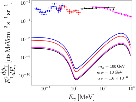
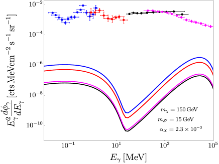
  Figure 8: Variation of differential photon flux as a function of the energy of the emitted photon for two different points which are allowed from the relic density constraint. Left panel: $E^{2}_{\gamma}$ weighted differential photon flux for $m_{\chi}=100\,{\rm GeV}$, $\alpha_{X}=1.6\times 10^{-3}$. Here blue, red, black, and magenta lines represent the differential photon flux calculated for the region of interest of INTEGRAL, COMPTEL, EGRET, and Fermi-LAT experimental collaborations respectively whereas the experimental data are shown by the data points with same color code. Right panel: $E^{2}_{\gamma}$ weighted differential photon flux for $m_{\chi}=150\,{\rm GeV}$ and $\alpha_{X}=2.3\times 10^{-3}$. The color codes are same as left panel. In both the plots we have considered $r=10^{-1}$.

• Inverse Compton scattering: The primary high energy electrons/positrons produced from the DM annihilation scatter with the low energy photons (such as CMB photons) and produce high energy gamma ray which is known as Inverse Compton Scattering (ICS) RevModPhys.42.237 . Following Cirelli:2009vg , we have calculated the $\gamma$ ray flux originating from the ICS with the ubiquitous CMB photons. In deriving the limits we have taken the primary spectra of $e^{-},\,e^{+}$ from PPPC4DMID for $5\,{\rm GeV}\leq m_{Z^{\prime}}/2\leq 100{\rm TeV}$ whereas for $m_{Z^{\prime}}/2<5\,{\rm GeV}$ we have only considered the monochromatic spectra of $e^{\pm}$ originating from the loop induced $Z^{\prime}\to e^{+}e^{-}$ decay.

Since $\gamma$ ray spectra from all of the above mentioned processes are calculated in the rest frame of $Z^{\prime}$ therefore using Eq. 79 we boost the $\gamma$ ray spectrum in the CoM frame of DM annihilation and in this frame the total differential $\gamma$ ray flux is given by

$$\dfrac{d\Phi_{\gamma}}{dE_{\gamma}}=\dfrac{d\Phi^{\rm prompt}_{\gamma}}{dE_{\gamma}}+\dfrac{d\Phi^{\rm ICS}_{\gamma}}{dE_{\gamma}}\,\,,$$ (37)

where $\dfrac{d\Phi^{\rm prompt}_{\gamma}}{dE_{\gamma}},\,\dfrac{d\Phi^{\rm ICS}_{\gamma}}{dE_{\gamma}}$ are the differential photon flux from the prompt gamma ray and ICS respectively.

In Fig. 8 we show the variation of $E_{\gamma}^{2}$ weighted differential flux as a function of the energy of the emitted photon for two relic density satisfied benchmark points. Here the fluxes are calculated for the region of interest (RoI) of the experimental collaboration which are given in Table 1. As one can see from the figure the flux for the RoI of INTEGRAL is larger than that of other RoIs. This is because of the fact that for cuspy DM profile such as NFW density profile the J-factor will be higher as we move towards the GC. Since the photon flux is directly proportional to $\bar{J}_{\rm ann}$, we get higher flux for higher values of J-factor. In Fig. 7, we show the constraints from the measurement of diffuse $\gamma$-ray background by INTEGRAL (purple region), COMPTEL (blue region), EGRET (violet region), and Fermi-LAT (cyan region) respectively.

Experiments	Region of Interest (RoI)
INTEGRAL Bouchet:2011fn	$|b|<15^{\circ},\,|l|<30^{\circ}$
COMPTEL comptel-kappadath	$|b|<20^{\circ},\,|l|<60^{\circ}$
EGRET Strong:2004de	$20^{\circ}<|b|<60^{\circ},\,0^{\circ}<l<360^{\circ}$
Fermi-LAT Fermi-LAT:2012edv	$8^{\circ}<|b|<90^{\circ},\,0^{\circ}<l<360^{\circ}$

Table 1: Region of interest of different experiments.

6 Constraints on the $L_{\mu}-L_{\tau}$ portal

6.1 BBN constraint

The number of relativistic degrees of freedom has been measured from the BBN observations and this is parametrized by defining a parameter $\rm N_{\rm eff}$. The presence of a new light particle can alter the number of relativistic degrees of freedom at the time of BBN if they are in thermal contact with the SM bath Heeck:2014zfa ; Knapen:2017xzo . Therefore the coupling and the mass of the new light particle can be constrained from $\Delta N_{\rm eff}\leq 1$ at the time BBN Mangano:2011ar .

In our model the presence of the dark vector boson $Z^{\prime}$ can modify the value of the effective degrees of freedom in two ways:

i) The mediator $Z^{\prime}$ can be in thermal equilibrium with the visible sector via $Z^{\prime}\leftrightarrow\bar{\nu}_{\mu}\nu_{\mu}$ and $Z^{\prime}\leftrightarrow\bar{\nu}_{\tau}\nu_{\tau}$ processes which enhances the value of $\Delta N_{\rm eff}$,

ii) Due to the presence of $Z^{\prime}$, neutrinos can remain in thermal equilibrium with the SM bath via $Z^{\prime}$ mediated processes $e^{+}e^{-}\leftrightarrow\bar{\nu}_{i}\nu_{i}$ and $e^{\pm}\nu_{i}(\bar{\nu}_{i})\leftrightarrow e^{\pm}\nu_{i}(\bar{\nu}_{i})$ where $i=\mu,\,\,\tau$. Since these processes are proportional to $\epsilon^{4}$ (at the cross section level) therefore the effect of them in the calculation of BBN bound is negligible compared to the $Z^{\prime}\leftrightarrow\bar{\nu}_{i}\nu_{i}$.

Therefore we have compared the reaction rate of $\bar{\nu}_{i}\nu_{i}\to Z^{\prime}$ ($Z^{\prime}\leftrightarrow\bar{\nu}_{i}\nu_{i}$ goes out-of-equilibrium when the inverse decay processes $\bar{\nu}_{i}\nu_{i}\to Z^{\prime}$ decouple) with the Hubble parameter $H$ at $T=1\,\rm MeV$. In Fig. 9 the blue dashed line represents the contour corresponding to $\Gamma/H|_{T=1\,\rm MeV}=1$. Besides, not to jeopardize the observations at the time BBN, the lifetime of $Z^{\prime}$ ($\tau_{Z^{\prime}}$) must be smaller than 1 second and the corresponding disallowed region is shown in Fig. 9 with light blue color.

6.2 SN1987A constraint

The presence of extra light degrees of freedom can enhance the rate of cooling of SN1987A which can be constrained from the observed neutrino luminosity after $1s$ of Supernova 1987A Dreiner:2013mua ; Chang:2016ntp . Since the luminosity of the neutrinos is $\mathcal{L}_{\nu}\simeq 3\times 10^{52}\,{\rm erg\,s^{-1}}$ and the mass of the core is $M_{\rm core}\sim 3\times 10^{33}\rm g$, the emissivity is $\mathcal{E}=\mathcal{L}_{\nu}/M_{\rm core}\sim 10^{19}\,{\rm erg\,g^{-1}\,s^{-1}}$. Thus emissivity due to the presence of a new degree of freedom must be smaller than $10^{19}\,{\rm erg\,g^{-1}\,s^{-1}}$ and it is known as “Raffelt criterion” Raffelt:1996wa .

In our model $Z^{\prime}$ can be produced from $\bar{\nu}_{i}\nu_{i}\rightarrow Z^{\prime}$ ($i=\mu,\,\tau$) which can contribute to the cooling of SN1987A. Thus we have calculated the emissivity ($\mathcal{E}_{\rm model}$) for these processes Escudero:2019gzq and the corresponding expression for the emissivity is given by

$$\mathcal{E_{\rm model}} \equiv \dfrac{1}{\rho_{\rm SN}}\dfrac{d\rho_{Z^{\prime}}}{dt}$$ (38)

$$= \dfrac{3T_{\rm SN}^{3}m_{Z^{\prime}}\sum_{i}\Gamma_{Z^{\prime}\to\bar{\nu}_{i}\nu_{i}}}{2\pi^{2}\rho_{\rm SN}}\int_{y}^{\infty}x\sqrt{x^{2}-y^{2}}\exp(-x)\exp\left(-\dfrac{yR_{\rm SN}\Gamma_{Z^{\prime}}}{\sqrt{x^{2}-y^{2}}}\right)dx\,\,.$$

Here $i=\{\mu,\,\tau,\,e\}$, $y=m_{Z^{\prime}}/T_{\rm SN}$, $\Gamma_{Z^{\prime}}$ is the total decay width of $Z^{\prime}$. The other parameters such as $T_{\rm SN}=30\rm MeV$ is the Supernovae (SN) temperature, the density of SN ($\rho_{\rm SN}$) is $3\times 10^{14}\rm g/cm^{3}$, and the radius of SN ($R_{\rm SN}$) is $13\rm km$.

Now we use the condition $\mathcal{E}_{\rm model}<\mathcal{E}$ to derive the bound in the $m_{Z^{\prime}}-\epsilon$ plane. The grey region of Fig. 9 is the disfavoured region from the SN1987A constraint. With the increase in the coupling $\epsilon$, the rate of energy loss will also increase and that will put an upper bound on the parameter $\epsilon$. However, if $\epsilon$ is sufficiently large, then the mean free path of $Z^{\prime}$ decreases. As a result, $Z^{\prime}$ produced from the inverse decay processes will be trapped inside SN and they will not contribute to the energy loss mechanism. Thus there will be a lower bound on $\epsilon$.

6.3 Beam dump experiments

The parameter space for a dark gauge boson of mass $\lesssim$ $1$ GeV and kinetic mixing $10^{-2}<\epsilon<10^{-8}$ can be constrained from the beam dump experiments as discussed in Bauer:2018onh . In our model the dark vector boson $Z^{\prime}$ can be produced from the bremsstrahlung processes via loop induced kinetic mixing between $\gamma$ and $Z^{\prime}$. Following Bauer:2018onh ; Bjorken:2009mm ; Mo:1968cg , we have derived the disallowed parameter space in $m_{Z^{\prime}}-\epsilon$ plane and the violet region of Fig. 9 represents the disallowed region.

6.4 White dwarf cooling

The White Dwarf (WD) cooling due to emission of neutrinos can be well described by the weak interactions. Thus any new interaction present in theory which contributes to the rate of cooling of WD can be constrained from the observations Dreiner:2013tja .

To derive the cooling constraint due to the presence of a massive vector boson $Z^{\prime}$, we calculate the effective Lagrangian for the new physics contribution to the neutrino-electron interaction as discussed in Dreiner:2013tja and the effective Lagrangian is given by

$$\mathcal{L}_{\rm NP}=-\mathcal{C}^{Z^{\prime}}_{\nu_{l}e}\left(\bar{\nu}_{l}\gamma_{\mu}P_{L}\nu_{l}\right)(\bar{e}\gamma^{\mu}e)\,\,.$$ (39)

Here

$$\mathcal{C}^{Z^{\prime}}_{\nu_{l}e}=\dfrac{\epsilon\sqrt{4\pi\alpha_{\rm em}}}{m_{Z^{\prime}}^{2}}\Pi(0)\,\,\,$$ (40)

where $\Pi(0)$ is given in Eq. 27.

As discussed in Dreiner:2013tja , The rate of WD cooling due to the new interaction must be smaller than the SM contribution to the WD cooling rate and it requires

$$\epsilon<5\times 10^{-5}\dfrac{m_{Z^{\prime}}}{1\,{\rm MeV}}\,\,.$$ (41)

Using Eq. 41 we have derived the WD cooling constraint and it is represented by the black dashed line in Fig. 9.

6.5 Stellar cooling

The dark vector $Z^{\prime}$ can be produced inside the stellar core and it may alter the observed rate of cooling. Therefore the properties of $Z^{\prime}$ can be constrained by requiring that the luminosity of $Z^{\prime}$ must be smaller than that of the photon luminosity. Using $Z^{\prime}$ interaction with the electromagnetic current via loop induced kinetic mixing, we have calculated the stellar cooling constraint as discussed in An:2013yfc ; Redondo:2008aa ; Hardy:2016kme . The relevant parameters of the stars for calculating the bounds such as temperature (T), radius (R), density ($\rho$), core composition, electron density ($n_{e}$), and luminosity ratio ($\mathcal{L}/\mathcal{L}_{\odot}$) are given in Table 2 Hardy:2016kme ; Dev:2020jkh . In Fig. 9 orange, red, and green regions are excluded from the cooling constraint of Sun, Horizontal Branch (HB) star, and Red giant respectively.

Star	T [keV]	R [cm]	$\rho$ [$\rm g\,cm^{-3}$]	Composition	$n_{e}$ [$\rm cm^{-3}$]	$\mathcal{L}/\mathcal{L}_{\odot}$
Sun	1	$7\times 10^{10}$	150	25%He 75%H	$10^{26}$	0.01
Horizontal Branch (HB) stars	8.6	$3.6\times 10^{9}$	$10^{4}$	${}^{4}{\rm He}_{2}$	$3\times 10^{27}$	5
Red Giant	10	$6\times 10^{8}$	$10^{6}$	${}^{4}{\rm He}_{2}$	$3\times 10^{29}$	2.8

Table 2: Required parameters for the calculation of stellar cooling limits from Sun, HB stars, and Red giant. Here $\mathcal{L_{\odot}}=4\times 10^{33}\,{\rm erg\,s^{-1}}$ is the solar luminosity.

6.6 Muon $g-2$ anomaly

From the recent measurement of muon $g-2$ by Fermilab Muong-2:2021ojo , it was found that there is a positive deviation of $(g-2)_{\mu}$ from SM prediction Davier:2017zfy ; Davier:2019can ; Aoyama:2020ynm . Combining the recent result of Fermilab with the older result of BNL E821 experiment Muong-2:2006rrc , the experimental value of $a_{\mu}\equiv\dfrac{1}{2}(g-2)_{\mu}$ differs from the SM prediction by $4.2\sigma$ and the deviation is given by Muong-2:2021ojo

$$\Delta a_{\mu}=(251\pm 59)\times 10^{-11}.$$ (42)

In our model, the dark vector boson $Z^{\prime}$ can contribute to the $(g-2)_{\mu}$ and the corresponding one loop integral is given below PhysRevD.64.055006 ; Ma:2001md ; Banerjee:2020zvi ; Fayet:2007ua ; Pospelov:2008zw .

$$\Delta a_{\mu} = \dfrac{\epsilon^{2}}{4\pi^{2}}\int_{0}^{1}\dfrac{m_{\mu}^{2}z(1-z)^{2}}{m_{\mu}^{2}(1-z)^{2}+m_{Z^{\prime}}^{2}z}dz\,\,,$$ (43)

where $m_{\mu}$ is the mass of the muon.

Using Eq. 43, we have calculated the allowed region (within $\pm 2\sigma$) of $m_{Z^{\prime}}-\epsilon$ plane in which the $(g-2)_{\mu}$ anomaly can be resolved by the dark vector boson $Z^{\prime}$ and the corresponding region is represented by cyan color in Fig. 9.

Figure 9: Parameter space in $m_{Z^{\prime}}-\epsilon$ plane for the dark gauge boson $Z^{\prime}$. The blue and black dashed lines are the BBN and white dwarf cooling constraint respectively. The disallowed region from $\tau_{Z^{\prime}}>1\rm s$ is shown by the light blue region. In the cyan region, $Z^{\prime}$ can resolve the Muon $g-2$ anomaly within $\pm 2\sigma$. The grey region is disallowed from SN1987A observation, Green, orange, and red region are disallowed from the cooling constraint of Red Giant, Sun, and HB star. Constraint on $Z^{\prime}$ from beam dump experiment is shown by the violet region and the yellow region is disallowed from the $5^{th}$ force experiment. The pink shaded region is excluded (at $95\%$ C.L.) Altmannshofer:2014pba from the neutrino trident production measurement at the CCFR experiment CCFR:1991lpl .

6.7 Fifth force constraint

The presence of a light $Z^{\prime}$ can modify the coloumb potential and the modification is parametrized as Jaeckel:2010ni

$$V(r)=\dfrac{\alpha_{\rm em}}{r}\left(1+|\Pi(m_{Z^{\prime}}^{2})|^{2}\exp(-m_{Z^{\prime}}r)\right)\,\,,$$ (44)

where $\Pi(m^{2}_{Z^{\prime}})$ can be calculated from Eq. 26.

As discussed in Bartlett:1988yy , due to the modification of the Coloumb potential, the change in Rydberg constant measurement for two different atomic transition ($\Delta R_{\infty}/R_{\infty}$) must be smaller than $10^{-10}$. Using this condition we have derived the fifth force constraint and the yellow region of Fig. 9 represents the disallowed region from the fifth force constraint.

7 Summary and Conclusion

In this work we have considered a gauged $U(1)_{X}$ secluded dark sector which contains a dark vector boson $Z^{\prime}$ and a Dirac fermion $\chi$ which is singlet under $SU(3)_{c}\otimes SU(2)_{L}\otimes U(1)_{Y}$ but charged under $U(1)_{X}$ gauge symmetry. We have also assumed that the SM sector is invariant under $U(1)_{L_{\mu}-L_{\tau}}$ gauge symmetry and we connect visible and dark sector through the kinetic mixing between $U(1)_{X}$ and $U(1)_{L_{\mu}-L_{\tau}}$ gauge boson. We have considered the portal coupling $\epsilon$ to be small enough so that the two sectors are thermally decoupled but the strength of the portal coupling is sufficient to exchange energy between the two sectors. Therefore the dark sector evolves non-adiabatically and in this framework we have studied the freeze-out of dark matter which is known as “Leak-in dark matter” scenario. In addition, we have explored other possible mechanisms for DM production such as freeze-in, and reannihilation. Since we have considered the dark sector to be thermally decoupled from the SM bath and it is internally thermalised therefore we have also shown the allowed region of the model parameter space in which both of these assumptions are valid.

Furthermore the detection prospect of our model has also been studied. We have investigated the constraints arising from direct detection, measurement of diffuse $\gamma$-ray background flux by INTEGRAL, COMPTEL, EGRET, Fermi-LAT, measurement of CMB anisotropy, and SIDM. Since there exists a $Z^{\prime}$ in our model therefore the mass and its coupling with the SM particles i.e. $\epsilon$ is constrained from various laboratory and astrophysical observations. In the light of theses observations we have also studied the constraints in $m_{Z^{\prime}}-\epsilon$ plane from BBN observations, SN1987A observations, beam dump experiment, white dwarf and stellar cooling as well as fifth force searches. We have found that the parameter space for the correct relic density is independent of $m_{Z^{\prime}}$ for $m_{\chi}/m_{Z^{\prime}}\gtrsim 10$, which is our parameter space of interest. The allowed region from the relic density constraint is consistent with the bounds in $m_{Z^{\prime}}-\epsilon$ plane for $m_{Z^{\prime}}>100\,{\rm MeV}$. Nevertheless, for $m_{Z^{\prime}}\lesssim 100\,{\rm MeV}$ there are significant constraints coming from beam dump experiment, SN1987A, BBN and star cooling. The bounds from direct detection, CMB anisotropy, SIDM, and the measurement of diffuse $\gamma$ ray background flux are dependent on $m_{Z^{\prime}}$ as well as $m_{\chi}$. We have discussed the dependence of these bounds on the mass ratio $r=m_{Z^{\prime}}/m_{\chi}$. We have found that for $r=10^{-1}$ the constraints from CMB and diffuse $\gamma$-ray observations are consistent with the relic density satisfied region and these constraints will be relaxed for smaller values of $r$. The SIDM and direct detection constraints for $r=10^{-3}$ are also consistent with the allowed region from the relic density constraint but these bounds will be significant for smaller values of $r$.

8 Acknowledgements

SG would like to thank Anirban Biswas for many useful discussions during the course of this work. SG would also like to thank University Grants Commission (UGC) for providing financial support in the form of a senior research fellowship. AT wishes to acknowledge the financial support provided by the Indian Association for the Cultivation of Science (IACS), Kolkata.

Appendix A $U(1)_{L_{\mu}-L_{\tau}}$ vector portal model

The $U(1)_{L_{\mu}-L_{\tau}}$ vector portal model can be described by the Eq. 1. To express Eq. 1 in the canonical form first we perform the following rotation.

$$\begin{pmatrix}\hat{Z}^{\prime}_{\rho}\\ \hat{Z}_{\mu\tau_{\rho}}\end{pmatrix}=\begin{pmatrix}\sec\delta&0\\ \tan\delta&1\end{pmatrix}\begin{pmatrix}\bar{Z^{\prime}}_{\rho}\\ \bar{Z}_{\mu\tau_{\rho}}\end{pmatrix}\,\,.$$ (45)

In $\left(\bar{Z}_{\mu\tau}~{}~{}~{}\bar{Z}^{\prime}\right)^{T}$ basis the gauge boson mass matrix has the following form.

$$\mathcal{M}^{2}_{\rm GB} = \hat{m}_{\mu\tau}^{2}\begin{pmatrix}1&&\tan\delta\\ \tan\delta&&\dfrac{\kappa^{2}}{\cos^{2}\delta}+\tan^{2}\delta\end{pmatrix}\,\,\,.$$ (46)

Now we perform an orthogonal rotation in $\left(\bar{Z}_{\mu\tau}~{}~{}~{}\bar{Z}^{\prime}\right)^{T}$ plane to diagonalise the gauge boson mass matrix. The orthogonal transformation is given by

$$\begin{pmatrix}\bar{Z}_{\mu\tau_{\rho}}\\ \bar{Z}^{\prime}_{\rho}\end{pmatrix} = \begin{pmatrix}\cos\beta&-\sin\beta\\ \sin\beta&\cos\beta\end{pmatrix}\begin{pmatrix}Z_{\mu\tau\rho}\\ Z^{\prime}_{\rho}\end{pmatrix}\,\,\,,$$ (47)

where the mixing angle is

$$\tan 2\beta = \dfrac{2\tan\delta}{1-\dfrac{\kappa^{2}}{\cos^{2}\delta}-\tan^{2}\delta}\,\,\,.$$ (48)

Therefore the diagonalised mass matrix in $\left(Z_{\mu\tau}~{}~{}~{}Z^{\prime}\right)^{T}$ basis has the following form.

$${\mathcal{M}^{2}_{\rm GB}}^{\rm dia.} = \begin{pmatrix}m_{\mu\tau}^{2}&0\\ 0&m^{\prime 2}\end{pmatrix}\,\,,$$ (49)

and the masses of the physical states are (assuming $\cos^{2}\delta\simeq 1$)

$$m_{\mu\tau}^{2} = \hat{m}_{\mu\tau}^{2}\left(1+\tan\beta\tan\delta\right)\,\,,$$

$$m^{\prime 2} = \dfrac{\hat{m}^{\prime 2}}{1+\tan\beta\tan\delta}\,\,\,.$$ (50)

Now we can express the mixing angle $\beta$ in terms of the physical masses of the gauge bosons and the mixing parameter $\delta$ as

$$\tan\beta = \dfrac{\tan\delta}{1-\hat{r}^{2}(1+\tan\beta\tan\delta)}\,\,,$$ (51)

where $\hat{r}=m^{\prime 2}/m_{\mu\tau}^{2}$.

Solving the above equation for $\tan\beta$ and choosing the condition $\beta\to 0$ as $\delta\to 0$ we have

$$\tan\beta = \dfrac{(1-\hat{r}^{2})-\sqrt{(1-\hat{r}^{2})^{2}-4\hat{r}^{2}\tan^{2}\delta}}{2\hat{r}^{2}\tan\delta}\,\,.$$ (52)

Assuming $\delta<<1$, we have arrived at the following relations.

$$\tan\beta = \dfrac{\tan\delta}{1-\hat{r}^{2}}\,\,,$$

$$\cos\beta = \dfrac{1-\hat{r}^{2}}{\sqrt{(1-\hat{r}^{2})^{2}+\tan^{2}\delta}}\,\,,$$

$$\sin\beta = \dfrac{\tan\delta}{\sqrt{(1-\hat{r}^{2})^{2}+\tan^{2}\delta}}\,\,.$$ (53)

Therefore we can write $\left(\hat{Z}_{\mu\tau}~{}~{}~{}\hat{Z}^{\prime}\right)^{T}$ in terms of $\left(Z_{\mu\tau}~{}~{}~{}Z^{\prime}\right)^{T}$ as follows.

$$\hat{Z}_{\mu\tau_{\rho}} = \left(\cos\beta+\tan\delta\sin\beta\right)Z_{\mu\tau_{\rho}}-\left(\sin\beta-\tan\delta\cos\beta\right)Z^{\prime}_{\rho}\,\,,$$

$$\hat{Z}^{\prime}_{\rho} = \dfrac{1}{\cos\delta}\left(\sin\beta Z_{\mu\tau_{\rho}}+\cos\beta Z^{\prime}_{\rho}\right)\,\,.$$ (54)

In the limit $\hat{r},\delta<<1$, we have

$$\hat{Z}_{\mu\tau_{\rho}} \simeq Z_{\mu\tau_{\rho}}-\hat{\epsilon}Z^{\prime}_{\rho}\,\,,$$

$$\hat{Z}^{\prime}_{\rho} \simeq Z^{\prime}_{\rho}+\tan\delta Z_{\mu\tau_{\rho}}\,\,\,,$$ (55)

where $\hat{\epsilon}=\hat{r}^{2}\tan\delta$.

Appendix B Calculation of $\mathcal{C}_{{\rm SM}\to Z^{\prime}}(T)$

The collision term $\mathcal{C}_{{\rm SM\to Z^{\prime}}}(T)$ defined in Eq. 8 for a process like ${\rm SM}(P_{1})+{\rm SM}(P_{2})\to{\rm SM}(P_{3})+Z^{\prime}(P_{4})$ (where SM denotes any SM fields) is given by

$$\mathcal{C}_{{\rm SM\to Z^{\prime}}}(T) = \int d\Pi_{i}E_{4}(2\pi)^{4}\delta^{4}(P_{1}+P_{2}-P_{3}-P_{4})\overline{|\mathcal{M}|^{2}}f_{\rm SM}(p_{1},T)f_{\rm SM}(p_{2},T)\,\,,$$ (56)

where the definition of all the quantities used in this equation are same as the definitions given in Eq. 8. Since SM fields are in thermal equilibrium therefore we use $f_{\rm SM}(p_{i},T)$ to be Maxwell-Boltzmann (MB) distribution. Using the MB distribution function for SM fields and the energy conservation, the above equation takes the following form.

$$\mathcal{C}_{{\rm SM\to Z^{\prime}}}(T) = \int d\Pi_{3}d\Pi_{4}E_{4}\exp\left(-\dfrac{E_{3}+E_{4}}{T}\right)4E_{3}E_{4}v\sigma_{34\to 12}\,\,,$$ (57)

where $\sigma_{34\to 12}$ is the annihilation cross section of the process ${\rm SM}(P_{3})+Z^{\prime}(P_{4})\to{\rm SM}(P_{1})+{\rm SM}(P_{2})$ and $4E_{3}E_{4}v$ is the usual flux factor. Following the technique given in Gondolo:1990dk we can write Eq. 57 as

$$\mathcal{C}_{{\rm SM\to Z^{\prime}}}(T) = \dfrac{g_{3}g_{4}\pi^{2}}{4(2\pi)^{6}}\int_{\Upsilon}^{\infty}d\,\hat{s}\int_{\sqrt{\hat{s}}}^{\infty}d\,E_{+}\int_{r_{1}}^{r_{2}}d\,E_{-}\left[\left(E_{+}^{2}-E_{-}^{2}\right)(E_{+}-E_{-})\right.$$ (58)

$$\left.~{}~{}~{}~{}~{}~{}~{}~{}~{}~{}~{}~{}~{}~{}~{}~{}~{}~{}~{}~{}~{}~{}~{}~{}~{}~{}~{}~{}~{}~{}~{}~{}~{}~{}~{}~{}~{}~{}~{}\times(\sigma v)_{34\to 12}\exp\left(-\dfrac{E_{+}}{T}\right)\right]\,\,,$$

where we define $E_{\pm}=\left(E_{3}\pm E_{4}\right)/2$, $r_{1}$ and $r_{2}$ are the lower and upper limit of $E_{-}$ respectively and the lower limit $\Upsilon$ of $\hat{s}$ integration are defined as follows.

$$\Upsilon = {{\rm Max}\left[(m_{1}+m_{2})^{2},(m_{3}+m_{Z^{\prime}})^{2}\right]}\,\,,$$

$$r_{1} = E_{+}\,\eta-2\sqrt{E_{+}^{2}-\hat{s}}\,\lambda\,\,\,,$$

$$r_{2} = E_{+}\,\eta+2\sqrt{E_{+}^{2}-\hat{s}}\,\lambda\,\,\,,$$

where

$$\lambda = \dfrac{\sqrt{\hat{s}-(m_{3}+m_{4})^{2}}\sqrt{\hat{s}-(m_{3}^{2}-m_{4})^{2}}}{2\hat{s}}\,\,,$$

$$\eta = \dfrac{m_{3}^{2}-m_{4}^{2}}{\hat{s}}\,\,.$$ (59)

Thus after performing the integration over $E_{+}$ and $E_{-}$ in Eq. 58 we can write the final form of the collision term as

$$\mathcal{C}_{{\rm SM}\to Z^{\prime}}(T) = \dfrac{g_{3}g_{4}T}{(2\pi)^{4}}\int_{\Upsilon}^{\infty}\lambda^{2}\,\hat{s}^{2}\,\left(1-\eta\right)\sigma_{34\to 12}\,K_{2}\left(\dfrac{\sqrt{\hat{s}}}{T}\right)d\,\hat{s}\,\,\,\,.$$ (60)

Appendix C Calculation of the reaction rate ($\Gamma$)

As discussed in section 3.2.1, to identify the relevant parameter space for the thermally decoupled dark sector we need to compare the total reaction rate for all processes discussed in section 3.1 with the hubble parameter.

For a process $A(P_{1})+Z^{\prime}(P_{2})\to B(P_{3})+C(P_{4})$ where $A,B,C$ are the SM particles, the reaction rate per $Z^{\prime}$ particle is given by

$$\Gamma_{AZ^{\prime}\to BC}=n^{\rm eq}_{A}(T)\langle\sigma v\rangle_{AZ^{\prime}\to BC}\,\,$$ (61)

where $n^{\rm eq}_{A}(T)$ is the equilibrium number density of A and the thermally averaged cross section of the above mentioned process can be written as follows Gondolo:1990dk .

$$\langle\sigma v\rangle_{aZ^{\prime}\to bc}=\dfrac{g_{A}{g_{Z}^{\prime}}}{n_{A}^{\rm eq}(T)n^{\rm eq}_{Z^{\prime}}(T)}\dfrac{T}{2(2\pi)^{4}}\int_{\Upsilon}^{\infty}\sigma(\hat{s})_{AZ^{\prime}\to BC}\,\tilde{\Gamma}(\hat{s},m_{A}^{2},m_{Z^{\prime}}^{2})\,{\rm K}_{1}\left(\dfrac{\sqrt{\hat{s}}}{T}\right)d\hat{s}\,\,,$$ (62)

where

$$\Upsilon = {\rm Max}\left[(m_{A}+m_{Z^{\prime}})^{2},(m_{B}+m_{C})^{2}\right]\,\,$$

$$\tilde{\Gamma} = \dfrac{\hat{s}^{2}-2\hat{s}(m_{A}^{2}+m_{Z^{\prime}}^{2})+(m_{A}^{2}-m_{Z^{\prime}}^{2})^{2}}{\sqrt{\hat{s}}}\,\,.$$ (63)

Therefore the total reaction rate per $Z^{\prime}$ is defined as

$$\Gamma=\sum_{\text{All channels}}\Gamma_{AZ^{\prime}\to BC}\,\,,$$ (64)

where the summation is taken over all the channels discussed in section 3.1.

Appendix D Thermalisation of the dark sector

In our analysis for the evolution of the dark sector, we have assumed that the dark sector is internally thermalised i.e. the DM $\chi$ and dark vector boson $Z^{\prime}$ is in thermal equilibrium. Therefore it is important to validate that the initial number density of $\chi$ and $Z^{\prime}$ produced from the SM bath and their interaction strength are sufficient to keep them in thermal equilibrium with different temperature from SM.

To study the allowed parameter space for the internal thermalisation first we study the production of $\chi$ and $Z^{\prime}$ from SM bath. The Boltzmann equation for the production of $\chi$ and $Z^{\prime}$ are as follows.

$$\frac{dn_{\chi}}{dt}+3Hn_{\chi} = \sum_{f}\mathcal{C}_{\bar{f}f\to\bar{\chi}\chi}(T)\,\,\,,$$

$$\frac{dn_{Z^{\prime}}}{dt}+3Hn_{Z^{\prime}} = \mathcal{C}_{{\rm SM}\to Z^{\prime}}(T)\,\,\,.$$ (65)

Here $H$ is the Hubble parameter defined in Eq. 7, $\mathcal{C}_{\bar{f}f\to\bar{\chi}\chi(T)}$ is the collision term for the DM production from SM bath and $f=\mu,\tau,\nu_{\mu},\nu_{\tau}$. The sum of the collision terms for the $Z^{\prime}$ production from the processes mentioned in section 3.1 is denoted by $\mathcal{C}_{{\rm SM}\to Z^{\prime}}(T)$.

Now we define the co-moving number density of $\chi$ and $Z^{\prime}$ as $Y_{\chi}=n_{\chi}/s$ and $Y_{Z^{\prime}}=n_{Z^{\prime}}/s$ where $s$ is the entropy density of the Universe. Now using the definition of $Y_{\chi}$ and $Y_{Z^{\prime}}$ we can write Eq. D as follows.

$$Y_{\chi}(T)=\sum_{f}\int_{T}^{T_{0}}\dfrac{\mathcal{C}_{\bar{f}f\to\bar{\chi}\chi}(\bar{T})}{\bar{T}H(\bar{T})s(\bar{T})}d\bar{T}\,\,\,,$$

$$Y_{Z^{\prime}}(T)=\int_{T}^{T_{0}}\dfrac{\mathcal{C}_{{\rm SM}\to Z^{\prime}}(\bar{T})}{\bar{T}H(\bar{T})s(\bar{T})}d\bar{T}\,\,\,,$$ (66)

where $T_{0}$ is the temperature of the Early Universe and $T_{0}>>T$.

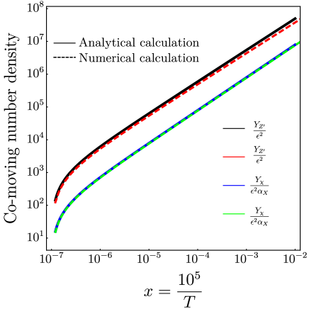
In the early Universe we have assumed $m^{2}/\hat{s}<<1$ where $\sqrt{\hat{s}}$ is the total energy of the initial state particles and $m$ represents the masses of the particles in the scattering process. Under this assumption we have calculated the collision terms analytically and in Fig.10 we have compared the result from the analytical and full numerical calculations. As one can see from the figure, the analytical estimate of $Y_{\chi}$ and $Y_{Z^{\prime}}$ are consistent with the full numerical calculation therefore from now on we will use the analytical results of $Y_{\chi}$ and $Y_{Z^{\prime}}$ for the remaining part of this section.

Figure 10: Numerical and analytical calculation of $Y_{\chi}$ and $Y_{Z^{\prime}}$.

Figure 11: Disallowed region from the thermalisation criteria in the $m_{\chi}-\epsilon$ plane for different values of $r$. The disallowed regions for $r=10^{-1},\,10^{-2},\,10^{-4}$, and $10^{-6}$ are denoted by yellow, green, grey, and pink color respectively.

Thus to check the thermalisation of the dark sector by $\bar{\chi}\chi\to Z^{\prime}Z^{\prime}$ process we need to calculate the region in which $\Gamma_{2\to 2}<H$, where we define $\Gamma_{2\to 2}$ as

$$\Gamma_{2\to 2}=s(T)\,{\rm Max}\left[Y_{\chi}(T)\langle\sigma v\rangle_{\bar{\chi}\chi\to Z^{\prime}Z^{\prime}},\,Y_{Z^{\prime}}(T)\langle\sigma v\rangle_{Z^{\prime}Z^{\prime}\to\bar{\chi}\chi}\right]\,\,.$$ (67)

However $2\to 3$ processes such as $\chi X\to\chi XZ^{\prime}$ $(X=\bar{\chi},Z^{\prime})$ can also thermalise the dark sector as discussed in Garny:2018grs . Though these $2\to 3$ processes are suppressed by another extra vertex factor $\alpha_{X}$ in comparison to the $2\to 2$ processes but for soft momentum exchange (i.e. the exchanged momentum in the propagator $\sim\sqrt{4\pi\alpha_{X}}T^{\prime}$) the rate of these $2\to 3$ processes are comparable to the rate of $2\to 2$ process. Since the time scale of both the processes are comparable therefore effect of several $2\to 2$ collision before the emission of $Z^{\prime}$ has to be taken into account. The emission rate of $Z^{\prime}$ is significantly modified due to the presence of multiple $2\to 2$ scattering and it is known as Landau-Pomeranchuk-Migdal (LPM) effect Migdal:1956tc ; Landau:1953gr .

Therefore following Garny:2018grs ; Arnold:2002zm , we have calculated the reaction rate of $2\to 3$ processes ($\Gamma_{2\to 3}$) and derive the disallowed region from the thermalisation criteria from the following relation.

$$\Gamma_{2\to 3}+\Gamma_{2\to 2}<H.$$ (68)

The disallowed region in the $m_{\chi}-\epsilon$ plane in which the dark sector is not internally thermalised, is shown in Fig. 11. In this figure we have considered four different values of $r$ which is defined as $r=m_{Z^{\prime}}/m_{\chi}$. In deriving the limit, we use Eq. 14, Eq. 15, and Eq. 19 to express $\alpha_{X}$ in terms of $m_{\chi},\,m_{Z^{\prime}}$, and $\epsilon$.

Appendix E Photon spectrum for final state radiation

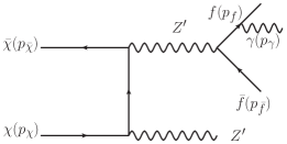
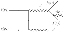
In our scenario the final state radiation occurs from one step cascade process shown in Fig. 12. The $\gamma$ ray spectrum in the rest frame of $Z^{\prime}$ is given by

$$\dfrac{dN^{\rm FSR}_{\gamma}}{dx_{\gamma}} = \dfrac{1}{\Gamma_{Z^{\prime}\to\bar{f}f}}\dfrac{\alpha_{\rm em}\epsilon^{2}m_{Z^{\prime}}}{192\pi^{2}}\int_{-1}^{1}\dfrac{d\cos\theta}{2}\int_{x_{f_{\rm min}}}^{x_{f_{\rm max}}}dx_{f}\mathcal{G}(x_{\gamma},x_{f},m_{f},{m_{Z}^{\prime}})\,\,,$$ (69)

where $x_{f}=2E_{f}/m_{Z^{\prime}}$, $x_{\gamma}=2E_{\gamma}/m_{Z^{\prime}}$. $E_{\gamma}$, $E_{f}$, and $\theta$ are the energy of the photon, energy of the fermion $f$, and angle of emission of $\gamma$ respectively and all of these quantities are measured in the rest frame of $Z^{\prime}$. The upper and lower limit of the $x_{f}$ integration are

$$x_{f_{\rm min}}=\dfrac{1}{2}\left[(2-x_{\gamma})-x_{\gamma}\sqrt{1-\dfrac{4m_{f}^{2}}{m_{Z^{\prime}}^{2}(1-x_{\gamma})}}\right]\,\,\,,$$

$$x_{f_{\rm max}}=\dfrac{1}{2}\left[(2-x_{\gamma})+x_{\gamma}\sqrt{1-\dfrac{4m_{f}^{2}}{m_{Z^{\prime}}^{2}(1-x_{\gamma})}}\right]\,\,\,.$$ (70)

The decay width of $Z^{\prime}$ into a pair of SM fermions is

$$\Gamma_{Z^{\prime}\to\bar{f}f} = \dfrac{\epsilon^{2}m_{Z^{\prime}}}{12\pi}\sqrt{1-\dfrac{4m_{f}^{2}}{m^{2}_{Z^{\prime}}}}\left(1+\dfrac{2m_{f}^{2}}{m^{2}_{Z^{\prime}}}\right)\,\,.$$ (71)

Now in Eq. 69 the function $\mathcal{G}(x_{\gamma},x_{f},m_{f},m_{Z^{\prime}})$ is given by

$$\mathcal{G}(x_{\gamma},x_{f},m_{f},m_{Z^{\prime}}) = g_{\mu\nu}X^{\mu\nu}\,\,\,,$$ (72)

where

$$X^{\mu\nu}=Tr \left[\left(\gamma_{\alpha}\dfrac{\not{p}_{f}+\not{p}_{\gamma}+m_{f}}{2p_{f}.p_{\gamma}}\gamma^{\mu}+\gamma^{\mu}\dfrac{-\not{p}_{\bar{f}}-\not{p}_{\gamma}+m_{f}}{2p_{\bar{f}}.p_{\gamma}}\gamma_{\alpha}\right)\left(\not{p}_{\bar{f}}-m_{f}\right)\right.$$ (73)

$$\left.\left(\gamma^{\nu}\dfrac{\not{p}_{f}+\not{p}_{\gamma}+m_{f}}{2p_{f}.p_{\gamma}}\gamma^{\alpha}+\gamma^{\alpha}\dfrac{-\not{p}_{\bar{f}}-\not{p}_{\gamma}+m_{f}}{2p_{\bar{f}}.p_{\gamma}}\gamma^{\nu}\right)\left(\not{p}_{f}+m_{f}\right)\right]\,\,\,.$$

Figure 12: Feynman diagrams for final state radiation

Using $E_{\bar{f}}=\dfrac{m_{Z^{\prime}}}{2}(2-x_{\gamma}-x_{f})$ in Eq. 73, we can write the final form of photon spectrum in the rest frame of $Z^{\prime}$ from Eq. 69 as follows.

$$\dfrac{dN^{\rm FSR}_{\gamma}}{dx_{\gamma}} = \dfrac{\alpha_{\rm em}}{8\pi\kappa(3-\kappa^{2})}\left[\mathcal{A}_{1}\ln\left(\dfrac{1+\lambda(x_{\gamma})}{1-\lambda(x_{\gamma})}\right)-\mathcal{A}_{2}\right]\,\,\,,$$ (74)

where

$$\kappa = \sqrt{1-\dfrac{4m_{f}^{2}}{m_{Z^{\prime}}^{2}}}\,\,,$$

$$\lambda(x_{\gamma}) = \sqrt{1-\dfrac{4m_{f}^{2}}{m^{2}_{Z^{\prime}}(1-x_{\gamma})}}\,\,\,,$$

$$\mathcal{A}_{1} = 8\left[\dfrac{(1+\kappa^{2})(3-\kappa^{2})}{x_{\gamma}}-2(3-\kappa^{2})+2x_{\gamma}\right]\,\,\,,$$

$$\mathcal{A}_{2} = 16\lambda(x_{\gamma})\left[\dfrac{(1-\kappa^{2})(3-\kappa^{2})}{x_{\gamma}(1-\lambda(x_{\gamma})^{2})}+x_{\gamma}\right]\,\,.$$ (75)

In the limit $\dfrac{4m_{f}^{2}}{m_{Z^{\prime}}^{2}}\to 0$, Eq. 74 takes the following form.

$$\dfrac{dN^{\rm FSR}_{\gamma}}{dx_{\gamma}} \simeq \dfrac{\alpha_{\rm em}}{\pi}\left(\dfrac{1+(1-x_{\gamma})^{2}}{x_{\gamma}}\right)\left[\ln\left(\dfrac{m^{2}_{Z^{\prime}}(1-x_{\gamma})}{m_{f}^{2}}\right)-1\right]\,\,\,.$$ (76)

Finally to calculate the $\gamma$ ray spectrum in the centre of mass (CoM) frame of DM annihilation Elor:2015tva we can write from Eq. 69

$$N^{\rm FSR}_{\gamma} = \int_{-1}^{1}\dfrac{d\cos\theta}{2}\int dx_{\gamma}\int dx_{f}\mathcal{G}(x_{\gamma},x_{f},m_{f},m_{Z^{\prime}})\,\,.$$ (77)

Now we use the following property of Dirac delta function.

$$\int dE^{0}_{\gamma}\delta\left(E^{0}_{\gamma}-\gamma_{Z^{\prime}}E_{\gamma}(1+\beta_{Z^{\prime}}\cos\theta)\right)=1\,\,\,,$$ (78)

where $E^{0}_{\gamma}$ is the photon energy in the CoM frame of DM annihilation, $\gamma_{Z^{\prime}}=\sqrt{s_{0}}/2m_{Z^{\prime}}$, $\beta_{Z^{\prime}}=\sqrt{1-\gamma^{-2}}$, and $\sqrt{s_{0}}$ is the total energy of the annihilating DM particles in the CoM frame.

Using Eq. 78 in Eq. 77 we can write the photon spectrum in the CoM frame of DM annihilation as follows.

$$\dfrac{dN^{\rm FSR}_{\gamma}}{dx^{0}_{\gamma}} = \dfrac{2}{\beta_{Z^{\prime}}}\int_{x_{\gamma_{\rm min}}}^{x_{\gamma_{\rm max}}}\dfrac{1}{x_{\gamma}}\dfrac{dN^{\rm FSR}_{\gamma}}{dx_{\gamma}}dx_{\gamma}\,\,\,,$$ (79)

where $x^{0}_{\gamma}=2E^{0}_{\gamma}/\sqrt{s_{0}}$, $x_{\gamma_{\rm min}}=\dfrac{2x^{0}_{\gamma}(1-\beta_{Z^{\prime}})}{\gamma_{Z^{\prime}}^{-2}}$, and $x_{\gamma_{\rm max}}={\rm Max}\left[1,\dfrac{2x^{0}_{\gamma}(1+\beta_{Z^{\prime}})}{\gamma_{Z^{\prime}}^{-2}}\right]$. The 2 factor in Eq. 79 arises due to production of two $Z^{\prime}$ from each DM annihilation process.

References

- (1) WMAP collaboration, Nine-Year Wilkinson Microwave Anisotropy Probe (WMAP) Observations: Cosmological Parameter Results, Astrophys. J. Suppl. 208 (2013) 19 [1212.5226].
- (2) Planck collaboration, Planck 2018 results. VI. Cosmological parameters, Astron. Astrophys. 641 (2020) A6 [1807.06209].
- (3) D. Clowe, M. Bradac, A. H. Gonzalez, M. Markevitch, S. W. Randall, C. Jones et al., A direct empirical proof of the existence of dark matter, Astrophys. J. Lett. 648 (2006) L109 [astro-ph/0608407].
- (4) Y. Sofue and V. Rubin, Rotation curves of spiral galaxies, Ann. Rev. Astron. Astrophys. 39 (2001) 137 [astro-ph/0010594].
- (5) M. Bartelmann and P. Schneider, Weak gravitational lensing, Phys. Rept. 340 (2001) 291 [astro-ph/9912508].
- (6) P. Gondolo and G. Gelmini, Cosmic abundances of stable particles: Improved analysis, Nucl. Phys. B 360 (1991) 145.
- (7) M. Srednicki, R. Watkins and K. A. Olive, Calculations of Relic Densities in the Early Universe, Nucl. Phys. B 310 (1988) 693.
- (8) G. Bertone, D. Hooper and J. Silk, Particle dark matter: Evidence, candidates and constraints, Phys. Rept. 405 (2005) 279 [hep-ph/0404175].
- (9) J. L. Feng, Dark Matter Candidates from Particle Physics and Methods of Detection, Ann. Rev. Astron. Astrophys. 48 (2010) 495 [1003.0904].
- (10) T. Lin, Dark matter models and direct detection, PoS 333 (2019) 009 [1904.07915].
- (11) L. Roszkowski, E. M. Sessolo and S. Trojanowski, WIMP dark matter candidates and searches—current status and future prospects, Rept. Prog. Phys. 81 (2018) 066201 [1707.06277].
- (12) G. Arcadi, M. Dutra, P. Ghosh, M. Lindner, Y. Mambrini, M. Pierre et al., The waning of the WIMP? A review of models, searches, and constraints, Eur. Phys. J. C 78 (2018) 203 [1703.07364].
- (13) L. J. Hall, K. Jedamzik, J. March-Russell and S. M. West, Freeze-In Production of FIMP Dark Matter, JHEP 03 (2010) 080 [0911.1120].
- (14) F. Elahi, C. Kolda and J. Unwin, UltraViolet Freeze-in, JHEP 03 (2015) 048 [1410.6157].
- (15) A. Biswas, D. Majumdar and P. Roy, Nonthermal two component dark matter model for Fermi-LAT -ray excess and 3.55 keV X-ray line, JHEP 04 (2015) 065 [1501.02666].
- (16) A. Biswas and A. Gupta, Freeze-in Production of Sterile Neutrino Dark Matter in U(1)B-L Model, JCAP 09 (2016) 044 [1607.01469].
- (17) N. Bernal, M. Heikinheimo, T. Tenkanen, K. Tuominen and V. Vaskonen, The Dawn of FIMP Dark Matter: A Review of Models and Constraints, Int. J. Mod. Phys. A 32 (2017) 1730023 [1706.07442].
- (18) A. Biswas, S. Ganguly and S. Roy, Fermionic dark matter via UV and IR freeze-in and its possible X-ray signature, JCAP 03 (2020) 043 [1907.07973].
- (19) B. Barman, D. Borah and R. Roshan, Effective Theory of Freeze-in Dark Matter, JCAP 11 (2020) 021 [2007.08768].
- (20) B. Barman, S. Bhattacharya and B. Grzadkowski, Feebly coupled vector boson dark matter in effective theory, JHEP 12 (2020) 162 [2009.07438].
- (21) M. Pospelov, A. Ritz and M. B. Voloshin, Secluded WIMP Dark Matter, Phys. Lett. B 662 (2008) 53 [0711.4866].
- (22) J. L. Feng, H. Tu and H.-B. Yu, Thermal Relics in Hidden Sectors, JCAP 10 (2008) 043 [0808.2318].
- (23) X. Chu, T. Hambye and M. H. G. Tytgat, The Four Basic Ways of Creating Dark Matter Through a Portal, JCAP 05 (2012) 034 [1112.0493].
- (24) A. Berlin, P. Gratia, D. Hooper and S. D. McDermott, Hidden Sector Dark Matter Models for the Galactic Center Gamma-Ray Excess, Phys. Rev. D 90 (2014) 015032 [1405.5204].
- (25) R. Foot and S. Vagnozzi, Dissipative hidden sector dark matter, Phys. Rev. D 91 (2015) 023512 [1409.7174].
- (26) T. Hambye, M. H. G. Tytgat, J. Vandecasteele and L. Vanderheyden, Dark matter from dark photons: a taxonomy of dark matter production, Phys. Rev. D 100 (2019) 095018 [1908.09864].
- (27) H. Baer, K.-Y. Choi, J. E. Kim and L. Roszkowski, Dark matter production in the early Universe: beyond the thermal WIMP paradigm, Phys. Rept. 555 (2015) 1 [1407.0017].
- (28) R. Foot and S. Vagnozzi, Diurnal modulation signal from dissipative hidden sector dark matter, Phys. Lett. B 748 (2015) 61 [1412.0762].
- (29) R. Foot and S. Vagnozzi, Solving the small-scale structure puzzles with dissipative dark matter, JCAP 07 (2016) 013 [1602.02467].
- (30) J. A. Evans, S. Gori and J. Shelton, Looking for the WIMP Next Door, JHEP 02 (2018) 100 [1712.03974].
- (31) J. A. Evans, C. Gaidau and J. Shelton, Leak-in Dark Matter, JHEP 01 (2020) 032 [1909.04671].
- (32) X.-G. He, G. C. Joshi, H. Lew and R. R. Volkas, Simplest Z-prime model, Phys. Rev. D 44 (1991) 2118.
- (33) X. G. He, G. C. Joshi, H. Lew and R. R. Volkas, NEW Z-prime PHENOMENOLOGY, Phys. Rev. D 43 (1991) 22.
- (34) S. Baek, N. G. Deshpande, X.-G. He and P. Ko, Muon anomalous and gauged models, Phys. Rev. D 64 (2001) 055006.
- (35) E. Ma, D. P. Roy and S. Roy, Gauged L(mu) - L(tau) with large muon anomalous magnetic moment and the bimaximal mixing of neutrinos, Phys. Lett. B 525 (2002) 101 [hep-ph/0110146].
- (36) H. Banerjee, B. Dutta and S. Roy, Supersymmetric gauged model for electron and muon anomaly, JHEP 03 (2021) 211 [2011.05083].
- (37) E. C. G. Stueckelberg, Interaction energy in electrodynamics and in the field theory of nuclear forces, Helv. Phys. Acta 11 (1938) 225.
- (38) H. Ruegg and M. Ruiz-Altaba, The Stueckelberg field, Int. J. Mod. Phys. A 19 (2004) 3265 [hep-th/0304245].
- (39) A. W. Strong, I. V. Moskalenko and O. Reimer, Diffuse galactic continuum gamma rays. A Model compatible with EGRET data and cosmic-ray measurements, Astrophys. J. 613 (2004) 962 [astro-ph/0406254].
- (40) S. C. Kappadath, Measurement of the cosmic diffuse gamma-ray spectrum from 800 keV to 30 MeV, Ph.D. thesis, University of New Hampshire, 1998.
- (41) L. Bouchet, A. W. Strong, T. A. Porter, I. V. Moskalenko, E. Jourdain and J.-P. Roques, Diffuse emission measurement with INTEGRAL/SPI as indirect probe of cosmic-ray electrons and positrons, Astrophys. J. 739 (2011) 29 [1107.0200].
- (42) Fermi-LAT collaboration, Fermi-LAT Observations of the Diffuse Gamma-Ray Emission: Implications for Cosmic Rays and the Interstellar Medium, Astrophys. J. 750 (2012) 3 [1202.4039].
- (43) S. Knapen, T. Lin and K. M. Zurek, Light Dark Matter: Models and Constraints, Phys. Rev. D 96 (2017) 115021 [1709.07882].
- (44) K. Griest and M. Kamionkowski, Unitarity Limits on the Mass and Radius of Dark Matter Particles, Phys. Rev. Lett. 64 (1990) 615.
- (45) C. Cheung, G. Elor, L. J. Hall and P. Kumar, Origins of Hidden Sector Dark Matter I: Cosmology, JHEP 03 (2011) 042 [1010.0022].
- (46) M. Bauer, P. Foldenauer and J. Jaeckel, Hunting All the Hidden Photons, JHEP 07 (2018) 094 [1803.05466].
- (47) A. Berlin, D. Hooper and S. D. McDermott, Simplified Dark Matter Models for the Galactic Center Gamma-Ray Excess, Phys. Rev. D 89 (2014) 115022 [1404.0022].
- (48) T. Araki, S. Hoshino, T. Ota, J. Sato and T. Shimomura, Detecting the gauge boson at Belle II, Phys. Rev. D 95 (2017) 055006 [1702.01497].
- (49) H. Banerjee and S. Roy, Signatures of supersymmetry and gauge bosons at Belle-II, Phys. Rev. D 99 (2019) 035035 [1811.00407].
- (50) XENON collaboration, Dark Matter Search Results from a One Ton-Year Exposure of XENON1T, Phys. Rev. Lett. 121 (2018) 111302 [1805.12562].
- (51) CRESST collaboration, First results from the CRESST-III low-mass dark matter program, Phys. Rev. D 100 (2019) 102002 [1904.00498].
- (52) XENON10 collaboration, A search for light dark matter in XENON10 data, Phys. Rev. Lett. 107 (2011) 051301 [1104.3088].
- (53) R. Essig, T. Volansky and T.-T. Yu, New Constraints and Prospects for sub-GeV Dark Matter Scattering off Electrons in Xenon, Phys. Rev. D 96 (2017) 043017 [1703.00910].
- (54) T. R. Slatyer, Indirect dark matter signatures in the cosmic dark ages. I. Generalizing the bound on s-wave dark matter annihilation from Planck results, Phys. Rev. D 93 (2016) 023527 [1506.03811].
- (55) Planck collaboration, Planck 2015 results. XIII. Cosmological parameters, Astron. Astrophys. 594 (2016) A13 [1502.01589].
- (56) S. W. Randall, M. Markevitch, D. Clowe, A. H. Gonzalez and M. Bradac, Constraints on the Self-Interaction Cross-Section of Dark Matter from Numerical Simulations of the Merging Galaxy Cluster 1E 0657-56, Astrophys. J. 679 (2008) 1173 [0704.0261].
- (57) S.-M. Choi, Y.-J. Kang and H. M. Lee, On thermal production of self-interacting dark matter, JHEP 12 (2016) 099 [1610.04748].
- (58) J. F. Navarro, C. S. Frenk and S. D. M. White, The Structure of cold dark matter halos, Astrophys. J. 462 (1996) 563 [astro-ph/9508025].
- (59) M. Cirelli, G. Corcella, A. Hektor, G. Hutsi, M. Kadastik, P. Panci et al., PPPC 4 DM ID: A Poor Particle Physicist Cookbook for Dark Matter Indirect Detection, JCAP 03 (2011) 051 [1012.4515].
- (60) M. Cirelli, N. Fornengo, B. J. Kavanagh and E. Pinetti, Integral X-ray constraints on sub-GeV Dark Matter, Phys. Rev. D 103 (2021) 063022 [2007.11493].
- (61) R. Essig, E. Kuflik, S. D. McDermott, T. Volansky and K. M. Zurek, Constraining Light Dark Matter with Diffuse X-Ray and Gamma-Ray Observations, JHEP 11 (2013) 193 [1309.4091].
- (62) Y. M. Bystritskiy, E. A. Kuraev, G. V. Fedotovich and F. V. Ignatov, The Cross sections of the muons and charged pions pairs production at electron-positron annihilation near the threshold, Phys. Rev. D 72 (2005) 114019 [hep-ph/0505236].
- (63) G. R. BLUMENTHAL and R. J. GOULD, Bremsstrahlung, synchrotron radiation, and compton scattering of high-energy electrons traversing dilute gases, Rev. Mod. Phys. 42 (1970) 237.
- (64) M. Cirelli and P. Panci, Inverse Compton constraints on the Dark Matter e+e- excesses, Nucl. Phys. B 821 (2009) 399 [0904.3830].
- (65) J. Heeck, Unbroken B – L symmetry, Phys. Lett. B 739 (2014) 256 [1408.6845].
- (66) G. Mangano and P. D. Serpico, A robust upper limit on from BBN, circa 2011, Phys. Lett. B 701 (2011) 296 [1103.1261].
- (67) H. K. Dreiner, J.-F. Fortin, C. Hanhart and L. Ubaldi, Supernova constraints on MeV dark sectors from annihilations, Phys. Rev. D 89 (2014) 105015 [1310.3826].
- (68) J. H. Chang, R. Essig and S. D. McDermott, Revisiting Supernova 1987A Constraints on Dark Photons, JHEP 01 (2017) 107 [1611.03864].
- (69) G. G. Raffelt, Stars as laboratories for fundamental physics: The astrophysics of neutrinos, axions, and other weakly interacting particles. The University of Chicago Press, 5, 1996.
- (70) M. Escudero, D. Hooper, G. Krnjaic and M. Pierre, Cosmology with A Very Light Lμ Lτ Gauge Boson, JHEP 03 (2019) 071 [1901.02010].
- (71) J. D. Bjorken, R. Essig, P. Schuster and N. Toro, New Fixed-Target Experiments to Search for Dark Gauge Forces, Phys. Rev. D 80 (2009) 075018 [0906.0580].
- (72) L. W. Mo and Y.-S. Tsai, Radiative Corrections to Elastic and Inelastic e p and mu p Scattering, Rev. Mod. Phys. 41 (1969) 205.
- (73) H. K. Dreiner, J.-F. Fortin, J. Isern and L. Ubaldi, White Dwarfs constrain Dark Forces, Phys. Rev. D 88 (2013) 043517 [1303.7232].
- (74) H. An, M. Pospelov and J. Pradler, New stellar constraints on dark photons, Phys. Lett. B 725 (2013) 190 [1302.3884].
- (75) J. Redondo, Helioscope Bounds on Hidden Sector Photons, JCAP 07 (2008) 008 [0801.1527].
- (76) E. Hardy and R. Lasenby, Stellar cooling bounds on new light particles: plasma mixing effects, JHEP 02 (2017) 033 [1611.05852].
- (77) P. S. B. Dev, R. N. Mohapatra and Y. Zhang, Stellar limits on light CP-even scalar, JCAP 05 (2021) 014 [2010.01124].
- (78) Muon g-2 collaboration, Measurement of the Positive Muon Anomalous Magnetic Moment to 0.46 ppm, Phys. Rev. Lett. 126 (2021) 141801 [2104.03281].
- (79) M. Davier, A. Hoecker, B. Malaescu and Z. Zhang, Reevaluation of the hadronic vacuum polarisation contributions to the Standard Model predictions of the muon and using newest hadronic cross-section data, Eur. Phys. J. C 77 (2017) 827 [1706.09436].
- (80) M. Davier, A. Hoecker, B. Malaescu and Z. Zhang, A new evaluation of the hadronic vacuum polarisation contributions to the muon anomalous magnetic moment and to , Eur. Phys. J. C 80 (2020) 241 [1908.00921].
- (81) T. Aoyama et al., The anomalous magnetic moment of the muon in the Standard Model, Phys. Rept. 887 (2020) 1 [2006.04822].
- (82) Muon g-2 collaboration, Final Report of the Muon E821 Anomalous Magnetic Moment Measurement at BNL, Phys. Rev. D 73 (2006) 072003 [hep-ex/0602035].
- (83) P. Fayet, U-boson production in e+ e- annihilations, psi and Upsilon decays, and Light Dark Matter, Phys. Rev. D 75 (2007) 115017 [hep-ph/0702176].
- (84) M. Pospelov, Secluded U(1) below the weak scale, Phys. Rev. D 80 (2009) 095002 [0811.1030].
- (85) W. Altmannshofer, S. Gori, M. Pospelov and I. Yavin, Neutrino Trident Production: A Powerful Probe of New Physics with Neutrino Beams, Phys. Rev. Lett. 113 (2014) 091801 [1406.2332].
- (86) CCFR collaboration, Neutrino tridents and W Z interference, Phys. Rev. Lett. 66 (1991) 3117.
- (87) J. Jaeckel and A. Ringwald, The Low-Energy Frontier of Particle Physics, Ann. Rev. Nucl. Part. Sci. 60 (2010) 405 [1002.0329].
- (88) D. F. Bartlett and S. Loegl, LIMITS ON AN ELECTROMAGNETIC FIFTH FORCE, Phys. Rev. Lett. 61 (1988) 2285.
- (89) M. Garny, A. Palessandro, M. Sandora and M. S. Sloth, Charged Planckian Interacting Dark Matter, JCAP 01 (2019) 021 [1810.01428].
- (90) A. B. Migdal, Bremsstrahlung and pair production in condensed media at high-energies, Phys. Rev. 103 (1956) 1811.
- (91) L. D. Landau and I. Pomeranchuk, Electron cascade process at very high-energies, Dokl. Akad. Nauk Ser. Fiz. 92 (1953) 735.
- (92) P. B. Arnold, G. D. Moore and L. G. Yaffe, Effective kinetic theory for high temperature gauge theories, JHEP 01 (2003) 030 [hep-ph/0209353].
- (93) G. Elor, N. L. Rodd and T. R. Slatyer, Multistep cascade annihilations of dark matter and the Galactic Center excess, Phys. Rev. D 91 (2015) 103531 [1503.01773].