An extended Krylov subspace method for decoding edge-based compressed images by homogeneous diffusion

Abstract

The heat equation is often used in order to inpaint dropped data in inpainting-based lossy compression schemes. We propose an alternative way to numerically solve the heat equation by an extended Krylov subspace method. The method is very efficient with respect to the direct computation of the solution of the heat equation at large times. And this is exactly what is needed for decoding edge-compressed pictures by homogeneous diffusion.

1 Introduction

Inpainting-based compression of images refers to the idea to identify prominent data in an image and to only store this data. All other data is disregarded and, when needed, reconstructed by inpainting. In particular, we will consider edge-based compressed images, where the edges of an image together with adjacent grey/colour data are stored (e.g. Carlsson88 ; Elder99 ; HuMo89 ; ZeRot86 ). This idea can be seen as a second-generation image coding method where the properties of the human visual system are taken into account (e.g. Reidetal97 ). The edge-based compression works very well for cartoon-like images (cf. Mainbergeretal11 ). In order to improve the quality of the reconstruction for natural images, we also compress images based on dithering. Dithering also works due to the perception of images by the human visual cortex. We will work with these two basic coding techniques. But since our new contribution refers to the decoding, more advanced coding techniques (e.g. Hoeltgenetal13 ; Mainbergeretal12 ) can easily be combined with our approach. We would also like to mention that, while our proposal deals with homogeneous diffusion, the proposed decoding method might be carried over to nonlinear partial differential equations used for inpainting by the help of exponential integrators, in which the linear part is solved as proposed in this work. More information on exponential integrators might be found in the survey hoacta10 and information on advanced image inpainting methods by partial differential equations can be found in inpaintingcarola15 .

In order to review the basic idea of inpainting-based compression of images, let $f:\Omega\rightarrow\mathbb{R}$ be a given grey-scale picture. $f({\bf x})$ refers to the intensity of light and $\Omega$ is the rectangular domain of the picture. In a colour picture, any channel is treated in the same way. After the compression of the picture, the intensities are only known on a subdomain $K\subset\Omega$. This splits the image in a know part $K$ and an unknown part $\Omega\backslash K$. To flag the stored pixels in an efficient way, we will use the function

$$c({\bf x})=\left\{\begin{array}[]{ll}1&\mbox{for}~{}{\bf x}\in K,\\ 0&\mbox{for}~{}{\bf x}\in\Omega\backslash K,\end{array}\right.$$

which we will refer to as inpainting mask. With the help of the inpainting mask, the compressed image $f_{c}$ can be written as $f_{c}=cf$. In the middle of figure 1, such a compressed picture of the picture on the left-hand side is shown. Only the pixels that are not black are stored. This data is sufficient for the reconstruction on the right-hand side of figure 1.

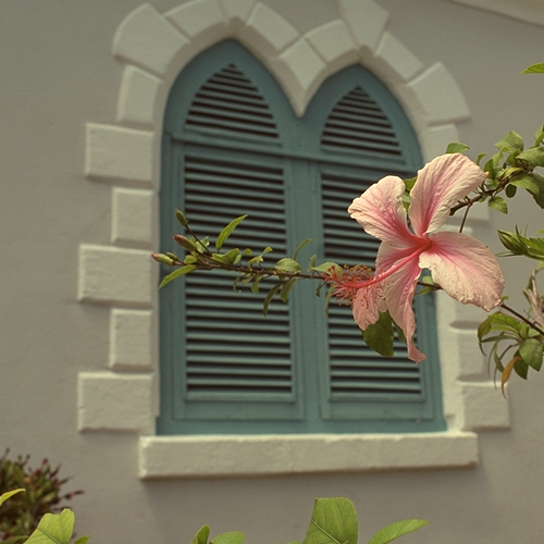
(a) original

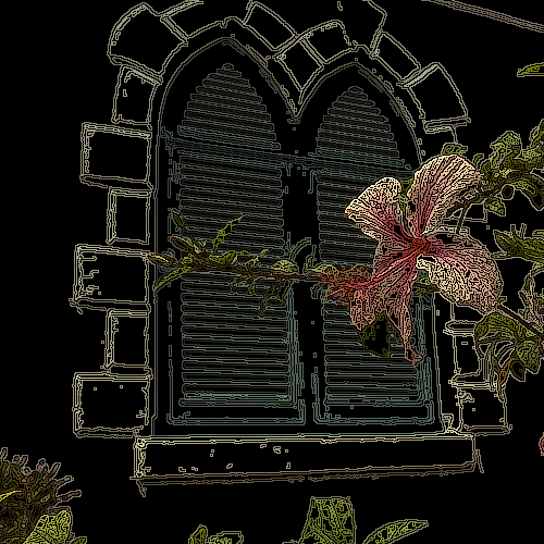
(b) compression

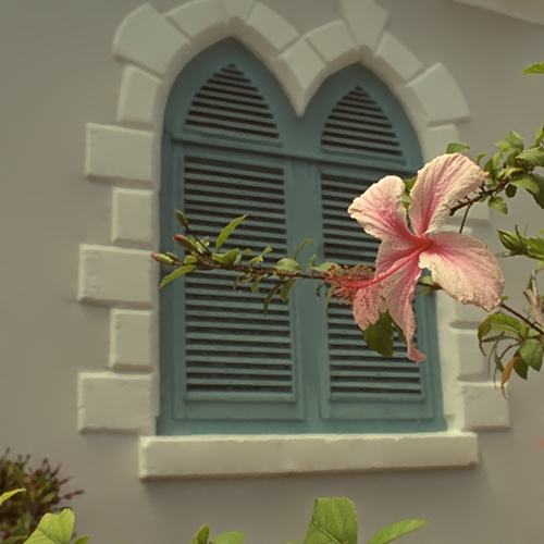
(c) reconstruction

Figure 1: Sketch of the compression scheme: in the encoding step the original picture is reduced to a subset, in the decoding phase the original is reconstructed from this subset.

For the reconstruction, we inpaint the missing data by the heat equation. The system reads

$$\partial_{t}u({\bf x},t) =(1-c({\bf x}))\Delta u({\bf x},t), \mbox{in}~{}\Omega\times[0,\infty),$$

$$\partial_{n}u({\bf x},t) =0, \mbox{in}~{}\partial\Omega\times[0,\infty),$$

with Neumann boundary conditions and the compressed image

$$u({\bf x},0)=c({\bf x})f({\bf x}),\qquad{\bf x}\in\Omega,$$

as initial data. The reconstructed picture is the solution $u({\bf x},t)$ of the above PDE at a large time $t$. Alternatively, one can compute the steady state $u^{S}({\bf x})=\lim_{t\rightarrow\infty}u({\bf x},t)$ of the diffusion process by solving the Poisson equation

$$c(u^{S}-f)-(1-c)\Delta u^{S} =0, \mbox{in}~{}\Omega,$$

$$\partial_{n}u^{S} =0, \mbox{in}~{}\partial\Omega.$$

Both approaches are widely used.

The new contribution is an efficient method to solve the discretised heat equation at a prescribed time $t$, directly. The discretisation of the heat equation leads to a huge system of ordinary differential equations

$${\bf y}^{\prime}=A{\bf y},\qquad{\bf y}(0)={\bf b}\,,$$ (1)

where ${\bf b}$ are the pixels of the compressed image written as a vector. The reconstructed image ${\bf y}(t)$ at time $t$ is given by the matrix exponential times the vector ${\bf b}$, i.e. ${\bf y}(t)=e^{tA}{\bf b}$.

Recently, rational Krylov subspace methods have been found to be an excellent choice for the approximation of the matrix exponential, that is, the solution of (1) at time $t$. Rational Krylov subspaces have been considered first by Axel Ruhe (e.g. Ruhe84 ; Ruhe98 ). They also turned out to be useful in inverse problems, in general (e.g. BreNoRe12 ; BuDoRei17 ; invkry ; RamRei19 ). If $A$ is an operator or an arbitrarily large matrix with a field-of-values in the left complex half-plane, the matrix exponential times a vector can be approximated reliably for an arbitrary time $t>0$ under reasonable assumptions on the vector (cf. GG13 ; GG14 ; ratkryphi11 ; GGautosmooth17 ). If the matrix $A$ is symmetric and the field-of-values is on the negative real axis, then rational Krylov methods are known that converge fast without any restrictions on the vector (cf. And81 ; marlis_jasper ). For finite subintervals of the negative real line, even super-linear convergence is obtained (cf. beckermann_guettel12 ).

Our matrix $A$ is not symmetric, but nevertheless allows for the use of a well-chosen rational Krylov subspace such that a fast convergence is obtained. We will approximate the solution of system (1) in extended Krylov subspaces of the form

$$\mathcal{E}_{m-1}((\gamma I-A)^{-1},{\bf b})$$ (2)

$$=\operatorname{span}\{{\bf b},A{\bf b},(\gamma I-A)^{-1}{\bf b},\cdots,(\gamma I-A)^{-m+2}{\bf b}\}\,,$$

where $\gamma>0$ (cf. Druskin_Knizhnerman98 ; GG13 ; KnizhSimoncini09 ). After the computation of an orthonormal basis $V_{m}\in\mathbb{R}^{n\times m}$ of this space and the compression $S_{m}=V_{m}^{T}AV_{m}$ of the huge matrix $A$ to a small $m\times m$ matrix, the Krylov approximation ${\bf f}_{m}$ is given by

$${\bf f}_{m}=\|{\bf b}\|V_{m}e^{tS_{m}}{\bf e}_{1},\qquad{\bf e}_{1}={\small\begin{pmatrix}1,0,\cdots,0\end{pmatrix}}^{T}\in\mathbb{R}^{m}\,.$$ (3)

This way, the solution of the huge system (1) is reduced to the solution of a small system of size $m\times m$, that is, to the computation of $e^{tS_{m}}{\bf e}_{1}$. For this purpose, methods for small matrices can be used (cf. AlMohyHigham11 , chapter 10 in highambook ). It will turn out, that a small $m$ is sufficient for arbitrary large matrices $A$. The choice of the subspace that leads to this favourable property is intricate due to two restrictions. A good error estimate is necessary in order to estimate the accuracy of the method and the computation of the vectors $(\gamma I-A)^{-m}{\bf b}$ requires the efficient solution of linear systems. This can be done by multigrid methods. In fact, it will turn out that only one solution of a linear system by the multigrid method is necessary for the purpose of reconstruction of compressed pictures. That is, the effort is comparable to the direct computation of the steady state of the system by a multigrid method as, for example, proposed in Mainbergeretal11 . In addition, the system that has to be solved in the Krylov method possesses a significantly smaller condition number. One also has the possibility to calculate reconstructed images at smaller times $t$ on purpose in order to regularise the computation.

The paper is organised as follows: After the introduction in this section, the encoding of pictures is briefly discussed in section 2. In section 3, the discretisation of the heat equation is described. The new decoding scheme and the main result that it works independent of the size of the picture for a given large time $t$ is shown in section 4. The multigrid method adapted to our purposes as an efficient method to solve the linear systems is discussed in section 5. Numerical experiments with the decoding scheme as illustration of our method are conducted in section 6. Here and everywhere, we will use pictures of the Kodak lossless colour image suite (cf. Kodak ). The work closes with a brief conclusion as section 7.

2 Encoding

In this section, we briefly describe the encoding. The basic idea is to determine a binary mask ${\bf c}$ of the same size as the picture that indicates which of the grey/colour values are stored. The choice of this mask determines the compression. The fewer pixels we have to store the higher will be the compression. The choice of the mask is also important for the obtainable quality of the reconstructed image. We consider two basic methods in order to determine a good mask for a later inpainting of the picture. For simplicity, we will not consider the generation of more elaborate masks by advanced coding techniques (e.g. Hoeltgenetal13 ; Mainbergeretal12 ). Our new decoding algorithm works with any mask ${\bf c}$. For the demonstration of our approach, the two basic masks will suffice.

2.1 Edge detection

Edges are very important for the perception of images by the human brain (cf. Marr76 ). Therefore, one often starts with detecting edge information in an image. One classic and often used idea is to identify edges as zero-crossings of the Laplacian of an image that has been smoothed by a Gaussian filter, the Marr-Hildreth edge detector (cf. MarrHildreth80 ). For a colour picture, ${\bf f}=(f_{1},f_{2},f_{3})^{T}$, the Laplacian is defined as the sum of the Laplacians over all channels:

$$\Delta{\bf f}=\sum_{k=1}^{3}\Delta f_{k}\,.$$

So, the idea is to store the pixels with large absolute value of this Laplacian. With respect to the inpainting approach by the heat equation, there is also a mathematical motivation for this idea. The steady state ${\bf u}^{S}$ satisfies $\Delta{\bf u}^{S}=0$ in regions where the image has been reconstructed. For the nearly steady state ${\bf u}(t)$ with a large time $t$, one has $\Delta{\bf u}(t)\approx 0$. This means that with respect to reconstructing an image by the heat equation, the error of the reconstructed image is large at places where the original image has large modulus of the Laplacian. Therefore the pixels of largest absolute value of the Laplacian should be stored and not reconstructed. In order to remove zero-crossings that arise from small oscillations in the image, the magnitude of the gradient $\nabla{\bf u}$ of the image at every pixel is used in addition. All edges are removed where the gradient is below a certain threshold. This is basically the idea of the Canny edge detector (cf. Canny86 ).

2.2 Dithering

If one uses the above idea for natural images, the highly textured parts of the image are strongly emphasised in contrast to the background. This can be seen in figure 2. The background seems to be too blurred. In order to improve the representation of smoother regions, in Belhachmietal09 , it is proposed to choose the edge data proportional to the absolute value of the Laplacian. In order to follow this suggestion, we use Floyd–Steinberg dithering (cf. FloStein76 ) for the modulus of the Laplacian. This method also allows for a simple method to prescribe the percentage of the pixels to be stored. For example, if one wishes to store $10\%$ of the pixels, the largest modulus of the Laplacian in the picture is scaled such that the average corresponds to a tenth of the value of a white pixel. If the maximal value of a white pixel is $255$, the average corresponds to $0.1\times 255=25.5$. In the course of the Floyd–Steinberg dithering, about 10% of the pixels will automatically be stored.

(a) original

(b) modulus Laplacian

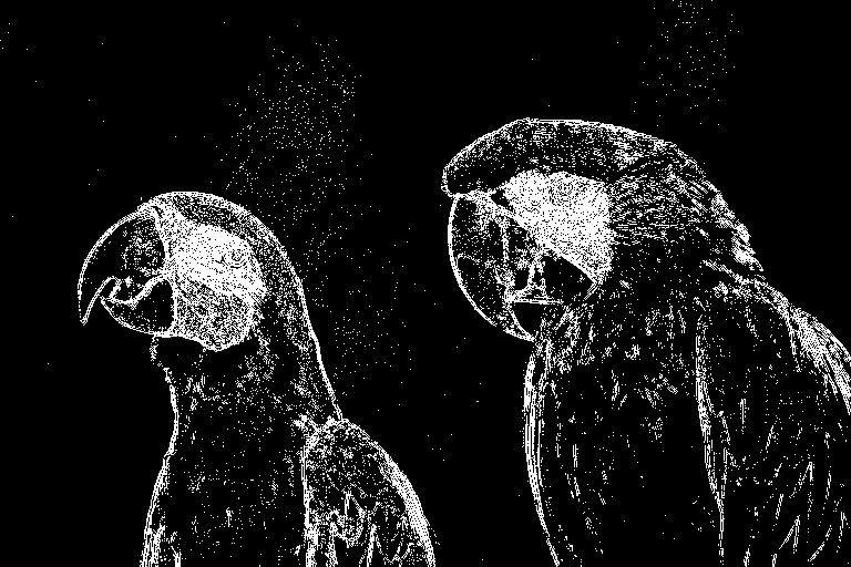
(c) threshold (10%)

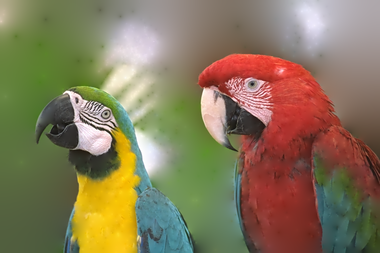
(d) reconstruction

Figure 2: The mask has been chosen such that 10% of the pixels with the largest modulus of the Laplacian are contained.

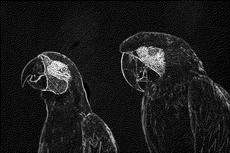
(a) dithering (10%)

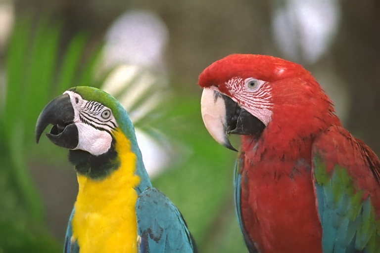
(b) reconstruction

Figure 3: The mask has been chosen such that the modulus of the Laplacian has been scaled to $10\%$ and dithering has been applied.

In the following, we will refer to the first method as edge-based compression and the second one as dithering-based compression. Dithering improves the display of the background in the reconstructed image as can be seen in figure 3. The edge-based compression is superior for cartoon-like images, vector graphics, pictograms, and letters, where the edges are the most important image feature. The dithering might be superior for natural images, as shown above.

2.3 Further compression

If one saves all important edges in the way proposed in Mainbergeretal11 , one stores more pixels as with the dithering approach. But this is mitigated by the fact that a subsampling of the edge-information is possible. Exactly by the algorithm proposed in Mainbergeretal11 , the two-dimensional signal is transformed to a one-dimensional one. Afterwards, since the one-dimensional signal shows more continuity, only every $d$-th value is stored. The masks generated by the edge-based approach are better suited for subsampling than the ones generated by dithering. A presmoothing to the one-dimensional signals might be applied in order to improve the subsampling even more.

The subsampled data is further compressed by uniform quantisation and then by applying an entropy coder. Since we mostly use the programming language Python in our numerical experiments, we applied the function savez_compressed of Python’s NumPy library as the entropy coder.

3 Discretisation

For decoding the compressed pictures, the $N_{x}\times N_{y}$ pixels of the original picture are interpreted as a finite-difference approximation to the heat equation. The mask ${\bf c}$ turns into a binary mask, where $1$ indicates that the pixel has been stored. Every such pixel is treated as a discretised Dirichlet boundary condition with the pixel value as the boundary value. Any boundary pixel, which is not a stored pixel, is treated as a homogeneous Neumann boundary. The Laplacian is discretised by the standard stencil

$$\Delta^{{\bf h}}\mathrel{\hat{=}}\begin{bmatrix}0&\frac{1}{h_{x}^{2}}&0\\ \frac{1}{h_{y}^{2}}&-\left(\frac{2}{h_{x}^{2}}+\frac{2}{h_{y}^{2}}\right)&\frac{1}{h_{y}^{2}}\\ 0&\frac{1}{h_{x}^{2}}&0\end{bmatrix}$$ (4)

with grid constants $h_{x},h_{y}$ in $x,y-$direction, respectively. The stencil is applied at any pixel which has not been stored. As usual in image processing, we will assume that the grid constants are one in both directions on the finest grid, which corresponds to the original picture. We illustrate the discretisation by the small example in figure 4. The discretised heat equation reads

$${\bf y}^{\prime}=A{\bf y},\qquad{\bf y}(0)={\bf b},$$ (5)

where $A$ and ${\bf b}$ are as follows.

$$A=\begin{bmatrix}-2&1&0&1&0&0\\ 1&-3&1&0&1&0\\ 0&0&0&0&0&0\\ 1&0&0&-2&1&0\\ 0&0&0&0&0&0\\ 0&0&1&0&1&-2\end{bmatrix}\qquad{\bf b}=\begin{bmatrix}0\\ 0\\ f_{3}^{h}\\ 0\\ f_{5}^{h}\\ 0\\ \end{bmatrix}.$$

The matrix $R$,

$$R=\begin{bmatrix}1&0&0&0&0&0\\ 0&1&0&0&0&0\\ 0&0&0&1&0&0\\ 0&0&0&0&0&1\end{bmatrix}$$

selects, by multiplication from the left-hand side, the rows of the matrix $A$ that correspond to pixels where the Laplacian stencil is applied. $R^{T}$ blows a vector that corresponds to the inner pixels up to the full size of our picture while setting the boundary pixels to zero. The projector $P=R^{T}R$ projects to the orthogonal complement of the space spanned by ${\bf b}$. As a consequence $PA=A$.

$$A_{\mbox{\scriptsize sym}}=RAR^{T}=\begin{bmatrix}-2&1&1&0\\ 1&-3&0&0\\ 1&0&-2&0\\ 0&0&0&-2\end{bmatrix},\qquad{\bf b}_{\mbox{\scriptsize sym}}=RA{\bf b}\,.$$

With the help of the matrices $R$ and $R^{T}$, respectively, a symmetric matrix $A_{\mbox{\scriptsize sym}}$ can be extracted from the matrix $A$ as well as a reduced vector ${\bf b}_{\mbox{\scriptsize sym}}$ that allow for an alternative representation of the solution of system (5) given in lemma 1.

Figure 4: Example of image with dimension $3\times 2$ and its row-major numbering

Lemma 1

The exact solution of equation (5) can be written as

$${\bf y}(t)=e^{tA}{\bf b}={\bf b}+R^{T}\left(t\varphi_{1}(tA_{\mbox{\scriptsize sym}}){\bf b}_{\mbox{\scriptsize sym}}\right)\,,$$ (6)

where $\varphi_{1}(z)=(e^{z}-1)/z$.

Proof

It is well known that the matrix exponential solves the ordinary differential equation (5). Hence, from here, we obtain

$${\bf y}(t) =e^{tA}{\bf b}={\bf b}+t\varphi_{1}(tA)A{\bf b}={\bf b}+t\varphi_{1}(tPA)PA{\bf b}$$

$$={\bf b}+R^{T}\left(t\varphi_{1}(tA_{\mbox{\scriptsize sym}}){\bf b}_{\mbox{\scriptsize sym}}\right)\,,$$

by $PA=A$ and the fact that

$$\varphi_{1}(R^{T}RA)R^{T}=R^{T}\varphi_{1}(RAR^{T})$$

according to corollary 1.34 on page $21$ in highambook .

In the alternative representation (6) of the solution, one can see that the stored pixels in ${\bf b}$ are never altered due to the properties of $R^{T}$, which is also true for the exact solution of (5), of course. Analogously to the proof of theorem 1 in Mainbergeretal11 , it follows by the Gershgorin disk theorem that $A_{\mbox{\scriptsize sym}}$ has only negative eigenvalues and hence is invertible. (Strictly speaking, $A_{\mbox{\scriptsize sym}}$ has only negative eigenvalues as soon as at least one boundary pixel exists in the interior of the rectangular domain of the picture.) From the stencil, one can easily read off that the matrix $A_{\mbox{\scriptsize sym}}$ is symmetric. Based on these facts, the following theorem shows that $(\gamma I-A)$ is invertible for all $\gamma>0$, which is crucial for our decoding method.

Lemma 2

For $\gamma>0$, we have

$$(\gamma I-A)^{-1}=\tfrac{1}{\gamma}I+\tfrac{1}{\gamma}R^{T}(\gamma I-A_{\mbox{\scriptsize sym}})^{-1}RA\,.$$

Proof

We compute

$$(\gamma I -A)\left(\tfrac{1}{\gamma}I+\tfrac{1}{\gamma}R^{T}(\gamma I-A_{\mbox{\scriptsize sym}})^{-1}RA\right)$$

$$=\tfrac{1}{\gamma}(\gamma I-A)-\tfrac{1}{\gamma}(\gamma I-A)R^{T}(\gamma I-A_{\mbox{\scriptsize sym}})^{-1}RA$$

$$=I-\tfrac{1}{\gamma}A-\tfrac{1}{\gamma}P(\gamma I-A)R^{T}(\gamma I-A_{\mbox{\scriptsize sym}})^{-1}RA$$

$$=I-\tfrac{1}{\gamma}A-\tfrac{1}{\gamma}R^{T}(\gamma I-A_{\mbox{\scriptsize sym}})(\gamma I-A_{\mbox{\scriptsize sym}})^{-1}RA$$

$$=I-\tfrac{1}{\gamma}A-\tfrac{1}{\gamma}PA=I\,.$$

4 Decoding by the extended Krylov subspace method

Extended Krylov subspaces for invertible matrices use the matrix as well as its inverse (e.g. Druskin_Knizhnerman98 ; GG13 ; KnizhSimoncini09 ). Let $C$ be an invertible matrix and ${\bf b}$ a vector of a suitable dimension. Then the extended Krylov subspace $\mathcal{E}_{p}^{q}(C,{\bf b})$ is defined as

$$\mathcal{E}_{p}^{q}(C,{\bf b})=\operatorname{span}\left\{{\bf b},C^{-1}{\bf b},\ldots,C^{-q}{\bf b},C{\bf b},\ldots,C^{p-1}{\bf b}\right\}\,.$$

Due to lemma 2, $\gamma I-A$ is invertible and hence we can set $C=(\gamma I-A)^{-1}$. We will use extended Krylov subspaces where $q$ is always one of the following form

$$\mathcal{E}_{m} ((\gamma I-A)^{-1},{\bf b})=\mathcal{E}_{m-1}^{1}((\gamma I-A)^{-1},{\bf b})$$

$$=\operatorname{span}\{{\bf b},A{\bf b},(\gamma I-A)^{-1}{\bf b},\cdots,(\gamma I-A)^{-m+2}{\bf b}\}\,.$$

Note, that we have used that $\operatorname{span}\{{\bf b},(\gamma I-A){\bf b}\}=\operatorname{span}\{{\bf b},A{\bf b}\}$, here. We start by computing the orthonormal basis $V_{m}\in\mathbb{R}^{n\times m}$ of the extended Krylov subspace by algorithm 1. Then, we compute the compression $S_{m}=V_{m}^{T}AV_{m}\in\mathbb{R}^{m\times m}$ of the large matrix $A$, and finally the Krylov approximation ${\bf f}_{m}$ as given in (3). In order to understand the properties of the Krylov algorithm, we study the algorithm via the symmetric matrix $A_{\mbox{\scriptsize sym}}$, the initial vector ${\bf b}_{\mbox{\scriptsize sym}}$, and the alternative solution representation (6).

Algorithm 1 Arnoldi-like algorithm

  Set ${\bf v}_{1}={\bf b}/\|{\bf b}\|$

  for m=1,2,3,… do

     if $m=1$ then

        $\tilde{{\bf v}}=A{\bf v}_{1}$

     else if $m=2$ then

        $\tilde{{\bf v}}=(\gamma I-A)^{-1}{\bf v}_{1}$

     else

        $\tilde{{\bf v}}=(\gamma I-A)^{-1}{\bf v}_{m}$

     end if

     for $j=1,\ldots,m$ do

        $\tilde{{\bf v}}=\tilde{{\bf v}}-(\tilde{{\bf v}},{\bf v}_{j}){\bf v}_{j}$

     end for

     ${\bf v}_{m+1}=\tilde{{\bf v}}/\|\tilde{{\bf v}}\|$

  end for

Algorithm 2 Symmetric Arnoldi

  Set ${\bf w}_{1}={\bf b}_{\mbox{\scriptsize sym}}/\|{\bf b}_{\mbox{\scriptsize sym}}\|$

  for m=1,2,3,… do

     $\tilde{{\bf w}}=(\gamma I-A_{\mbox{\scriptsize sym}})^{-1}{\bf w}_{m}$

     if $m=1$ then

        $\tilde{{\bf w}}=\tilde{{\bf w}}-(\tilde{{\bf w}},{\bf w}_{1}){\bf w}_{1}$

     else

        for $j=m-1,m$ do

           $\tilde{{\bf w}}=\tilde{{\bf w}}-(\tilde{{\bf w}},{\bf w}_{j}){\bf w}_{j}$

        end for

     end if

     ${\bf w}_{m+1}=\tilde{{\bf w}}/\|\tilde{{\bf w}}\|$

  end for

The computation of the basis $V_{m}$ by algorithm 1 can be compared with the symmetric Arnoldi method for a related Krylov subspace as outlined in lemma 3.

Lemma 3

Let $W_{m-1}=[{\bf w}_{1},\cdots,{\bf w}_{m-1}]$ be the Arnoldi basis for the Krylov subspace $\mathcal{K}_{m-1}((\gamma I-A_{\mbox{\scriptsize sym}})^{-1},{\bf b}_{\mbox{\scriptsize sym}})$ according to algorithm 2. Then, the orthonormal basis for the extended Krylov subspace

$$\mathcal{E}_{m} ((\gamma I-A)^{-1},{\bf b})$$

$$=\operatorname{span}\{{\bf b},A{\bf b},(\gamma I-A)^{-1}{\bf b},\cdots,(\gamma I-A)^{-m+2}{\bf b}\}$$

according to algorithm 1 reads

$$V_{m}=\left[{\bf v}_{1},\ldots,{\bf v}_{m}\right]=\left[{\bf v}_{1},R^{T}W_{m-1}\right]\,,\qquad{\bf v}_{1}=\frac{1}{\|{\bf b}\|}{\bf b}\,.$$

Proof

The idea of the following proof is to compare the Arnoldi-like algorithm 1 with the Arnoldi algorithm (cf. algorithm 6.1 in Saaditer ) for the standard Krylov space $\mathcal{K}_{m-1}((\gamma I-A_{\mbox{\scriptsize sym}})^{-1},{\bf b}_{\mbox{\scriptsize sym}})$, whose definition can be found in section 6.2 of Saaditer . The Arnoldi algorithm is the same as algorithm 2 with the difference that the for-loop $j$ runs from $j=0,\ldots,m$. The Arnoldi-like algorithm leads to the following. Let ${\bf v}_{1}=\frac{1}{\|{\bf b}\|}{\bf b}$, which is the obvious start. Then

$$A{\bf v}_{1} =\frac{1}{\|{\bf b}\|}A{\bf b}=\frac{1}{\|{\bf b}\|}R^{T}{\bf b}_{\mbox{\scriptsize sym}},$$

$$h_{1,1} ={\bf v}_{1}^{T}A{\bf v}_{1}=\frac{1}{\|{\bf b}\|^{2}}{\bf b}^{T}A{\bf b}=\frac{1}{\|{\bf b}\|^{2}}{\bf b}^{T}PA{\bf b}=0,$$

$$\tilde{{\bf v}}_{2} =A{\bf v}_{1}-h_{1,1}{\bf v}_{1}=\frac{1}{\|{\bf b}\|}R^{T}{\bf b}_{\mbox{\scriptsize sym}},$$

$${\bf v}_{2} =\frac{1}{\|\tilde{{\bf v}}_{2}\|}\tilde{{\bf v}}_{2}=R^{T}\frac{1}{\|{\bf b}_{\mbox{\scriptsize sym}}\|}{\bf b}_{\mbox{\scriptsize sym}}=R^{T}{\bf w}_{1}\,.$$

Our statement is proved for $m=2$. For $m=3$, the calculation reads

$$\tilde{{\bf v}}_{3} =(\gamma I-A)^{-1}{\bf v}_{1}-\left({\bf v}_{2}^{T}(\gamma I-A)^{-1}{\bf v}_{1}\right){\bf v}_{2}$$

$$\qquad-\left({\bf v}_{1}^{T}(\gamma I-A)^{-1}{\bf v}_{1}\right){\bf v}_{1}$$

$$=\left(\tfrac{1}{\gamma}I+\tfrac{1}{\gamma}R^{T}(\gamma I-A_{\mbox{\scriptsize sym}})^{-1}RA\right){\bf v}_{1}$$

$$\qquad-\left({\bf v}_{2}^{T}\left(\tfrac{1}{\gamma}I+\tfrac{1}{\gamma}R^{T}(\gamma I-A_{\mbox{\scriptsize sym}})^{-1}RA\right){\bf v}_{1}\right){\bf v}_{2}$$

$$\qquad-\left({\bf v}_{1}^{T}\left(\tfrac{1}{\gamma}I+\tfrac{1}{\gamma}R^{T}(\gamma I-A_{\mbox{\scriptsize sym}})^{-1}RA\right){\bf v}_{1}\right){\bf v}_{1}$$

$$=\tfrac{1}{\gamma}R^{T}(\gamma I-A_{\mbox{\scriptsize sym}})^{-1}RA{\bf v}_{1}$$

$$\qquad-\tfrac{1}{\gamma}\left({\bf v}_{2}^{T}R^{T}(\gamma I-A_{\mbox{\scriptsize sym}})^{-1}RA{\bf v}_{1}\right){\bf v}_{2}$$

$$\qquad-\tfrac{1}{\gamma}\underbrace{\left({\bf v}_{1}^{T}R^{T}(\gamma I-A_{\mbox{\scriptsize sym}})^{-1}RA{\bf v}_{1}\right)}_{=0}{\bf v}_{1}$$

$$=\tfrac{\|{\bf b}_{\mbox{\scriptsize sym}}\|}{\gamma\|{\bf b}\|}R^{T}\Big{(}(\gamma I-A_{\mbox{\scriptsize sym}})^{-1}{\bf w}_{1}$$

$$\qquad-\left({\bf w}_{2}^{T}(\gamma I-A_{\mbox{\scriptsize sym}})^{-1}{\bf w}_{1}\right){\bf w}_{1}\Big{)}$$

$$=\frac{\|{\bf b}_{\mbox{\scriptsize sym}}\|}{\gamma\|{\bf b}\|}R^{T}\tilde{{\bf w}}_{2}\,.$$

Hence,

$${\bf v}_{3}=\frac{1}{\|\tilde{{\bf v}}_{3}\|}\tilde{{\bf v}}_{3}=R^{T}\frac{\tilde{{\bf w}}_{2}}{\|\tilde{{\bf w}}_{2}\|}=R^{T}{\bf w}_{2}\,.$$

From here, induction will complete the proof for $k\geq 3$

$$\tilde{{\bf v}}_{k+1} =(\gamma I-A)^{-1}{\bf v}_{k}-\Big{(}\sum_{j=2}^{k}\big{(}{\bf v}_{j}^{T}(\gamma I-A)^{-1}{\bf v}_{k}\big{)}{\bf v}_{j}\,\Big{)}$$

$$\qquad-\underbrace{\big{(}{\bf v}_{1}^{T}(\gamma I-A)^{-1}{\bf v}_{k}\big{)}}_{=0}{\bf v}_{1}$$

$$=(\gamma I-A)^{-1}R^{T}{\bf w}_{k-1}$$

$$\qquad-\sum_{j=2}^{k}\big{(}{\bf w}_{j-1}^{T}R(\gamma I-A)^{-1}R^{T}{\bf w}_{k-1}\big{)}R^{T}{\bf w}_{j-1}$$

$$=R^{T}(\gamma I-A_{\mbox{\scriptsize sym}})^{-1}{\bf w}_{k-1}$$

$$\qquad-\sum_{j=1}^{k-1}\big{(}{\bf w}_{j}^{T}(\gamma I-A_{\mbox{\scriptsize sym}})^{-1}{\bf w}_{k-1}\big{)}R^{T}{\bf w}_{j}$$

$$=R^{T}\Big{(}(\gamma I-A_{\mbox{\scriptsize sym}})^{-1}{\bf w}_{k-1}$$

$$\qquad-\sum_{j=1}^{k-1}\big{(}{\bf w}_{j}^{T}(\gamma I-A_{\mbox{\scriptsize sym}})^{-1}{\bf w}_{k-1}\big{)}{\bf w}_{j}\Big{)}$$

$$=R^{T}\tilde{{\bf w}}_{k}$$

Finally,

$${\bf v}_{k+1}=\frac{\tilde{{\bf v}}_{k+1}}{\|\tilde{{\bf v}}_{k+1}\|}=R^{T}\frac{\tilde{{\bf w}}_{k}}{\|\tilde{{\bf w}}_{k}\|}=R^{T}{\bf w}_{k}\,.$$

We have now proved our statement for the Arnoldi algorithm. Since the matrix $(\gamma I-A_{\mbox{\scriptsize sym}})^{-1}$ is symmetric, the Arnoldi algorithm automatically reduces to the symmetric Arnoldi algorithm (cf. section 6.6 in Saaditer ).

The relation between algorithm 1 and algorithm 2 stated in lemma 3 has another important obvious consequence, which is noted in corollary 1.

Corollary 1

Due to lemma 3, the for-loop $j$ in algorithm 1 only needs to run over $j=m-1,m$ for $m>3$.

That things change for $m>3$ can also be seen in the proof of lemma 3. The following lemma relates the compression $S_{m}=V_{m}^{T}AV_{m}$ of $A$ in the extended Krylov subspace to the compression $\widetilde{S}_{m-1}=W_{m-1}^{T}A_{\mbox{\scriptsize sym}}W_{m-1}$ of $A_{\mbox{\scriptsize sym}}$ in the Krylov space $\mathcal{K}_{m-1}((\gamma I-A_{\mbox{\scriptsize sym}})^{-1},{\bf b}_{\mbox{\scriptsize sym}})$.

Lemma 4

Let $\widetilde{S}_{m-1}=W_{m-1}^{T}A_{\mbox{\scriptsize sym}}W_{m-1}$. Then, for $S_{m}=V_{m}^{T}AV_{m}$, one can find

$$S_{m}=\begin{bmatrix}0&0\\ {\bf u}&\tilde{S}_{m-1}\\ \end{bmatrix},\quad{\bf u}=\frac{1}{\|{\bf b}\|}W_{m-1}^{T}{\bf b}_{\mbox{\scriptsize sym}}=\frac{\|{\bf b}_{\mbox{\scriptsize sym}}\|}{\|{\bf b}\|}{\bf e}_{1},$$

with ${\bf e}_{1}\in\mathbb{R}^{m-1}$, and therefore, $\gamma I-S_{m}$ is invertible for all $\gamma>0$.

Proof

By lemma 3, one obtains

$$S_{m} =V_{m}^{T}AV_{m}=\begin{bmatrix}\frac{1}{\|{\bf b}\|}{\bf b}&R^{T}W_{m-1}\end{bmatrix}^{T}A\begin{bmatrix}\frac{1}{\|{\bf b}\|}{\bf b}&R^{T}W_{m-1}\end{bmatrix}$$

$$=\begin{bmatrix}\frac{1}{\|{\bf b}\|}{\bf b}^{T}\\ W_{m-1}^{T}R\end{bmatrix}\begin{bmatrix}\frac{1}{\|{\bf b}\|}A{\bf b}&AR^{T}W_{m-1}\end{bmatrix}$$

$$=\begin{bmatrix}\frac{1}{\|{\bf b}\|^{2}}{\bf b}^{T}A{\bf b}&\frac{1}{\|{\bf b}\|}{\bf b}^{T}AR^{T}W_{m-1}\\ \frac{1}{\|{\bf b}\|}W_{m-1}^{T}RA{\bf b}&W_{m-1}^{T}RAR^{T}W_{m-1}\end{bmatrix}\,.$$

Since $A{\bf v}$ has zeros where ${\bf b}$ has entries and vice versa, ${\bf b}^{T}A{\bf b}=0$ and $\frac{1}{\|{\bf b}\|}{\bf b}^{T}AR^{T}W_{m-1}={\bf 0}$ is a zero vector of length $m-1$. Furthermore,

$${\bf u} =\frac{1}{\|{\bf b}\|}W_{m-1}^{T}RA{\bf b}=\frac{1}{\|{\bf b}\|}W_{m-1}^{T}{\bf b}_{\mbox{\scriptsize sym}}$$

$$=\frac{\|{\bf b}_{\mbox{\scriptsize sym}}\|}{\|{\bf b}\|}W_{m-1}^{T}{\bf w}_{1}=\frac{\|{\bf b}_{\mbox{\scriptsize sym}}\|}{\|{\bf b}\|}{\bf e}_{1}$$

and

$$\tilde{S}_{m-1}=W_{m-1}^{T}RAR^{T}W_{m-1}=W_{m-1}^{T}A_{\mbox{\scriptsize sym}}W_{m-1}\,.$$

Hence

$$\gamma I-S_{m}=\begin{bmatrix}\gamma&0\\ -{\bf u}&\gamma I-\tilde{S}_{m-1}\end{bmatrix}$$

is invertible, since $\gamma>0$ and $\tilde{S}_{m-1}$ is a symmetric, negative-definite matrix, by lemma 5, and $\gamma I-\tilde{S}_{m-1}$ therefore is a symmetric positive-definite matrix.

Lemma 5

$\tilde{S}_{m-1}$ is a symmetric and negative-definite matrix.

Proof

The symmetry follows directly from the symmetry of $A_{\mbox{\scriptsize sym}}$:

$$\tilde{S}_{m-1}^{T} =\left(W_{m-1}^{T}A_{\mbox{\scriptsize sym}}W_{m-1}\right)^{T}=W_{m-1}^{T}A_{\mbox{\scriptsize sym}}^{T}W_{m-1}$$

$$=W_{m-1}^{T}A_{\mbox{\scriptsize sym}}W_{m-1}=\tilde{S}_{m-1}\,.$$

Since $A_{\mbox{\scriptsize sym}}$ is symmetric and has only negative eigenvalues, the field-of-values of $A_{\mbox{\scriptsize sym}}$ is given as

$$W(A_{\mbox{\scriptsize sym}})=[\lambda_{\mbox{\scriptsize min}},\lambda_{\mbox{\scriptsize max}}]\subset(-\infty,0),$$

where

$$\lambda_{\mbox{\scriptsize min}}=\min_{\lambda\in\sigma(A_{\mbox{\scriptsize sym}})}\lambda,\qquad\lambda_{\mbox{\scriptsize max}}=\max_{\lambda\in\sigma(A_{\mbox{\scriptsize sym}})}\lambda\,,$$

and $\sigma(A_{\mbox{\scriptsize sym}})$ is the set of eigenvalues. Hence, for the field-of-values of $\tilde{S}_{m-1}$,

$$W(\tilde{S}_{m-1}) =\left\{\frac{{\bf y}^{H}\tilde{S}_{m-1}{\bf y}}{{\bf y}^{H}{\bf y}}~{}\big{|}~{}0\neq{\bf y}\in\mathbb{C}^{n-1}\right\}$$

$$\subset W(A_{\mbox{\scriptsize sym}})=[\lambda_{\mbox{\scriptsize min}},\lambda_{\mbox{\scriptsize max}}]\,,$$

since

$$\frac{{\bf y}^{H}W_{m-1}^{H}A_{\mbox{\scriptsize sym}}W_{m-1}{\bf y}}{{\bf y}^{H}{\bf y}} =\frac{{\bf y}^{H}W_{m-1}^{H}A_{\mbox{\scriptsize sym}}W_{m-1}{\bf y}}{{\bf y}^{H}W_{m-1}^{H}W_{m-1}{\bf y}}$$

$$=\frac{{\bf x}^{H}A_{\mbox{\scriptsize sym}}{\bf x}}{{\bf x}^{H}{\bf x}}\,,\qquad{\bf x}=W_{m-1}{\bf y}\,.$$

Hence, since $\sigma(\tilde{S}_{m-1})\subset W(\tilde{S}_{m-1})$, all eigenvalues of $\tilde{S}_{m-1}$ are negative and

$$\frac{{\bf y}^{H}\tilde{S}_{m-1}{\bf y}}{\|{\bf y}\|^{2}}<0\,\qquad\mbox{for all}\quad{\bf y}\neq{\bf 0}\,,$$

and therefore

$${\bf y}^{H}\tilde{S}_{m-1}{\bf y}<0,\qquad\mbox{for all}\quad{\bf y}\neq{\bf 0}\,,$$

which means that $\tilde{S}_{m-1}$ is negative definite.

The following theorem states that the boundary pixels are correctly set in the first Krylov step and not altered afterwards due to the properties of the matrix $R^{T}$. An alternative representation of the Krylov approximation is given with the help of the $\varphi_{1}$-function analogous to lemma 1.

Theorem 4.1

The Krylov approximation to the matrix exponential times vector, $e^{tA}{\bf b}$, in the extended Krylov subspace $\mathcal{E}_{m}((\gamma I-A)^{-1},{\bf b})$ reads

$$\|{\bf b}\|V_{m}e^{tS_{m}}{\bf e}_{1}={\bf b}+R^{T}\left(\|{\bf b}_{\mbox{\scriptsize sym}}\|W_{m-1}t\varphi_{1}(t\tilde{S}_{m-1}){\bf e}_{1}\right)\,.$$

Proof

With the help of lemma 4, one obtains

$$e^{tS_{m}} =\sum_{k=0}^{\infty}\frac{t^{k}}{k!}S_{m}^{k}=\sum_{k=0}^{\infty}\frac{t^{k}}{k!}\begin{pmatrix}0&0\\ {\bf u}&\tilde{S}_{m-1}\end{pmatrix}^{k}$$

$$=I+\sum_{k=1}^{\infty}\frac{t^{k}}{k!}\begin{pmatrix}0&0\\ \tilde{S}_{m-1}^{k-1}{\bf u}&\tilde{S}_{m-1}^{k}\end{pmatrix}\,,$$

and hence

$$e^{tS_{m}}{\bf e}_{1} ={\bf e}_{1}+\sum_{k=1}^{\infty}\frac{t^{k}}{k!}\begin{pmatrix}0&0\\ \tilde{S}_{m-1}^{k-1}{\bf u}&\tilde{S}_{m-1}^{k}\end{pmatrix}{\bf e}_{1}$$

$$={\bf e}_{1}+\begin{pmatrix}0\\ \sum_{k=1}^{\infty}\frac{t^{k}}{k!}\tilde{S}_{m-1}^{k-1}{\bf u}\end{pmatrix}$$

$$=\begin{pmatrix}1\\ t\varphi_{1}(t\tilde{S}_{m-1}){\bf u}\end{pmatrix}=\begin{pmatrix}1\\ \frac{\|{\bf b}_{\mbox{\scriptsize sym}}\|}{\|{\bf b}\|}t\varphi_{1}(t\tilde{S}_{m-1}){\bf e}_{1}\end{pmatrix}$$

Finally, one obtains

$$\|{\bf b}\| V_{m}e^{tS_{m}}{\bf e}_{1}$$

$$=\|{\bf b}\|\begin{bmatrix}{\bf v}_{1}&R^{T}W_{m-1}\end{bmatrix}\begin{bmatrix}1\\ \frac{\|{\bf b}_{\mbox{\scriptsize sym}}\|}{\|{\bf b}\|}t\varphi_{1}(t\tilde{S}_{m-1}){\bf e}_{1}\end{bmatrix}$$

$$=\|{\bf b}\|{\bf v}_{1}+\|{\bf b}\|R^{T}W_{m-1}\left(\frac{\|{\bf b}_{\mbox{\scriptsize sym}}\|}{\|{\bf b}\|}t\varphi_{1}(t\tilde{S}_{m-1}){\bf e}_{1}\right)$$

$$={\bf b}+R^{T}\left(\|{\bf b}_{\mbox{\scriptsize sym}}\|W_{m-1}t\varphi_{1}(t\tilde{S}_{m-1}){\bf e}_{1}\right).$$

The comparison of the exact solution with the Krylov approximation via the alternative representation by the $\varphi_{1}$-function leads to the error bound in theorem 4.2. The $\varphi_{1}$-function can by approximated uniformly for matrices/operators with field-of-values in the left half-plane, which could be proved in ratkryphi11 . Here we obtain even better bounds due to the symmetry of the matrix at which the function is evaluated.

Theorem 4.2

The error of the rational Krylov approximation ${\bf f}_{m}=\|{\bf b}\|V_{m}e^{tS_{m}}{\bf e}_{1}$ in the extended Krylov subspace $\mathcal{E}_{m-1}((\gamma I-tA)^{-1},{\bf b})$ with $\gamma>0$ to the solution of (1) reads, for $m\geq 2$ and $t>0$,

$$\|e^{tA}{\bf b}-{\bf f}_{m}\|\leq 2tE_{m}(\gamma)\|{\bf b}_{\mbox{\scriptsize sym}}\|,$$

with

$$E_{m}(\gamma)=\min_{r\in\mathcal{R}_{m-1}}\|\varphi_{1}-r\|_{(-\infty,0]}\,,$$

where $\|\cdot\|_{(-\infty,0]}$ designates the supremum norm on $(-\infty,0]$ and the space

$$\mathcal{R}_{m-1}=\left\{\frac{p_{m-2}}{(\gamma-\cdot)^{m-2}}~{}|~{}p_{m-2}\in\mathcal{P}_{m-2}\right\}$$

is the space of rational functions of the indicated form and dimension $m-1$. Here, $\mathcal{P}_{m-2}$ is the space of polynomials with degree less than or equal to $m-2$.

Proof

With lemma 1 and theorem 4.1, one obtains

$$e^{tA}{\bf b}-{\bf f}_{m}$$

$$=tR^{T}(\varphi_{1}(tA_{\mbox{\scriptsize sym}}){\bf b}_{\mbox{\scriptsize sym}}-\|{\bf b}_{\mbox{\scriptsize sym}}\|W_{m-1}\varphi_{1}(t\tilde{S}_{m-1}){\bf e}_{1})\,.$$

Hence, by the exactness property in the Krylov space $\mathcal{K}_{m-1}((\gamma I-A_{\mbox{\scriptsize sym}})^{-1},{\bf b}_{\mbox{\scriptsize sym}})$, namely

$$\tilde{r}(A_{\mbox{\scriptsize sym}}){\bf b}_{\mbox{\scriptsize sym}}=\|{\bf b}_{\mbox{\scriptsize sym}}\|W_{m-1}\tilde{r}(\tilde{S}_{m-1}){\bf e}_{1}\,,$$

for all $\tilde{r}\in\mathcal{R}_{m-1}$, one obtains (by using $\tilde{r}(\cdot)=r(t\cdot)$, $t>0$, as rational function)

$$\|e^{tA}{\bf b} -{\bf f}_{m}\|$$

$$\leq t\|(\varphi_{1}(tA_{\mbox{\scriptsize sym}})-r(tA_{\mbox{\scriptsize sym}})){\bf b}_{\mbox{\scriptsize sym}}\|$$

$$\qquad+t\|{\bf b}_{\mbox{\scriptsize sym}}\|\|(r(t\tilde{S}_{m-1})-\varphi_{1}(t\tilde{S}_{m-1})){\bf e}_{1}\|$$

$$\leq 2t\|{\bf b}_{\mbox{\scriptsize sym}}\|\cdot\min_{r\in\mathcal{R}_{m-1}}\max_{z\in(-\infty,0]}|\varphi_{1}(z)-r(z)|\,.$$

Note that $E_{m}(\gamma)$ does neither depend on the chosen $t>0$ nor on the size of the matrix $A$. With exactly the same ideas as in marlis_jasper , table 1 of optimal values of $\gamma$ with respect to the minimisation of the error can be numerically computed with the help of a simple transform and the Remez algorithm. Note that there is a subtle issue about scaling. One has to use the Krylov subspace as given in the theorem. Alternatively, one might use the space $\mathcal{E}_{m}((\tilde{\gamma}I-A)^{-1},{\bf b})$ with $\tilde{\gamma}=\gamma_{\mbox{\scriptsize opt}}/t$ for the simple reason that $\mathcal{E}_{m}((\gamma I-tA)^{-1},{\bf b})=\mathcal{E}_{m}((\frac{\gamma}{t}I-A)^{-1},{\bf b})$. We refer the reader to marlis_jasper for details.

Table 1: Numerical approximation to the optimal value of $\gamma$, $\gamma_{\mbox{\scriptsize opt}}$, and the error $E_{m}^{m}(\gamma_{\mbox{\scriptsize opt}})$ for the optimal choice of $\gamma$, dimension $m$ of the extended Krylov subspace, and $\#lss$ linear system solves by the multigrid method.

.

$\#lss$	$m$	$E_{m}(\gamma_{\mbox{\scriptsize opt}})$	$\gamma_{\mbox{\scriptsize opt}}$
$1$	$3$	$2.6\cdot 10^{-2}$	$1.5$
$2$	$4$	$6.6\cdot 10^{-3}$	$3.5$
$3$	$5$	$2.2\cdot 10^{-3}$	$5.5$
$4$	$6$	$6.9\cdot 10^{-4}$	$3.5$
$5$	$7$	$2.0\cdot 10^{-4}$	$5$
$6$	$8$	$8.9\cdot 10^{-5}$	$7$
$7$	$9$	$2.8\cdot 10^{-5}$	$8.5$
$8$	$10$	$1.0\cdot 10^{-5}$	$6.5$
$9$	$11$	$3.8\cdot 10^{-6}$	$8.5$
$10$	$12$	$1.1\cdot 10^{-6}$	$10$
$11$	$13$	$5.3\cdot 10^{-7}$	$8.5$
$12$	$14$	$1.8\cdot 10^{-7}$	$10$
$13$	$15$	$5.7\cdot 10^{-8}$	$11.5$
$14$	$16$	$2.5\cdot 10^{-8}$	$10$
$15$	$17$	$8.6\cdot 10^{-9}$	$11.5$
$16$	$18$	$3.1\cdot 10^{-9}$	$13$
$17$	$19$	$1.3\cdot 10^{-9}$	$11.5$
$18$	$20$	$4.8\cdot 10^{-10}$	$13$
$19$	$21$	$1.9\cdot 10^{-10}$	$14.5$
$20$	$22$	$8.3\cdot 10^{-11}$	$16$

We illustrate the bound and the necessity of the scaling numerically. We use an all-white square grey-scale picture of size $1024\times 1024$. The Canny-like edge detector then produces the mask with all boundary pixels set to one and all interior points set to zero. That is, the compressed picture has a white boundary and all pixels in the interior are black. For this simple example, the solution of the inpainting by the heat equation can be computed at any time $t>0$ by fast transforms. In figure 5, we show the error bound of theorem 4.1 with the optimal choices of $\gamma$ according to table 1 as a black solid line and the error of the approximation with respect to the Krylov subspace $\mathcal{E}_{m}((\tilde{\gamma}I-A)^{-1},{\bf b})$ with $\tilde{\gamma}=\gamma_{\mbox{\scriptsize opt}}/t$ as in the theorem as green circle-marked line for $t=25$, $t=10^{3}$, $t=10^{5}$, and $t=10^{7}$, respectively. The red diamond-marked line corresponds to the extended Krylov subspace $\mathcal{E}_{m}((I-A)^{-1},{\bf b})$. That is, $\gamma$ is set to one and not scaled. For $t=25$, the approximation for small dimensions of the space with $\gamma$ fixed to one is clearly worse than the error bound in contrast to the properly scaled Krylov subspace. For $t=10^{3}$, $t=10^{5}$, and $t=10^{7}$, the approximation of the space with $\gamma$ fixed to one does not improve for larger dimensions of the Krylov subspace, either. For $t=10^{7}$ the approximation in the extended Krylov subspace with optimal $\gamma$ approximates the steady state, and here the worst-case error bound of theorem 4.1 is clearly too pessimistic. The Krylov subspace method reveals another of its strengths, the fact that these approximations are nearly optimal and can therefore be significantly better than worst-case error bounds.

Figure 5: Error bound of theorem 4.1 (black) solid line for the optimal choice of $\gamma$, error of the extended Krylov subspace approximation to the compressed all-white picture for the optimal $\gamma$ (green) circle-marked line, and error of the extended Krylov subspace with $\gamma$ fixed to one (red) diamond-marked line for $t=25$ on the top left-hand side, $t=10^{3}$ on the top right-hand side, $t=10^{5}$ on the bottom left-hand side, $t=10^{7}$ on the bottom right-hand side.

Since the eye can not distinguish very small deviations, the error bound in theorem 4.1 and our experiment suggest that an extended Krylov subspace of a small dimension is sufficient for image processing purposes. This will be confirmed in section 6 by numerical experiments with real pictures.

5 Implementation details

For the efficient computation of ${\bf v}^{{\bf h}}=(\gamma I-A^{{\bf h}})^{-1}{\bf b}^{{\bf h}}$, we use the multigrid method applied to the system

$$B^{{\bf h}}{\bf v}^{{\bf h}}={\bf b}^{{\bf h}},\qquad B^{{\bf h}}=(\gamma I-A^{{\bf h}})\,.$$

The superscript ${\bf h}$ indicates that the matrices and vectors belong to the finest grid which corresponds to the original image. In order to efficiently implement the multigrid method, we operate on the discrete images following mainly the ideas in Bruhnetal05 and Mainbergeretal11 . For the application of the multigrid method, we look at a fine grid $\Omega^{\bf h}$ with $N^{\bf h}=N_{x}^{\bf h}\times H_{y}^{\bf h}$ pixels, where $H_{x}^{\bf h}$ and $H_{y}^{\bf h}$ correspond to the number of pixels in $x$- and $y$-direction, respectively. The grid spacing is denoted by ${\bf h}=(h_{x},h_{y})^{T}$. On the finest grid $(h_{x},h_{h})^{T}=(1,1)^{T}$, which is a popular choice in image processing. For the next coarser grid, one would like to double the grid spacing in both directions. This is only possible for powers of two. In order to include other grids, we define the coarser grid $\Omega^{\bf H}$ with the spacings ${\bf H}=(H_{x},H_{y})^{T}$, with

$$H_{x}=h_{x}\frac{N_{x}^{\bf h}}{N_{x}^{\bf H}},\qquad H_{y}=h_{y}\frac{N_{y}^{\bf h}}{N_{y}^{\bf H}}\,,$$

where $N_{x}^{\bf H}=\lceil N_{x}^{\bf h}/2\rceil$ and $N_{y}^{\bf H}=\lceil N_{y}^{\bf h}/2\rceil$ are the number of pixels in each direction in the coarse grid. For the restriction, the coarse pixel is the average of the fine pixels according to the area of the fine pixel that contributes to the coarse pixel. The prolongation reverses this process. For the restriction matrix $I_{\bf h}^{\bf H}$ and the prolongation matrix $I_{\bf H}^{\bf h}$, one has the relation

$$I_{\bf h}^{\bf H}=\alpha(I_{\bf H}^{\bf h})^{T},\qquad\alpha=\frac{N_{x}^{\bf H}N_{y}^{\bf H}}{N_{x}^{\bf h}N_{y}^{\bf h}}=\frac{h_{x}h_{y}}{H_{x}H_{y}}\,.$$

Restriction and prolongation are illustrated in figure 6.

Figure 6: Example for the restriction and prolongation

Since we have two different sorts of pixels, we also have to apply the restriction and prolongation to our binary inpainting mask ${\bf c}$. We therefore adapt the restriction of the inpainting by applying the element-wise sign function to the restricted inpainting mask

$${\bf c}^{\bf H}=\text{sgn}(I_{\bf h}^{\bf H}{\bf c}^{\bf h}).$$

This is also illustrated in figure 7.

Figure 7: Example for the restriction applied to the inpainting mask

With these two definitions, we obtain a natural definition of the coarse matrix $A^{\bf H}$. We can just use again the standard stencil for the Laplace operator with respect to the grid spacing ${\bf H}=(H_{x},H_{y})^{T}$. For the multigrid method, we also need to compute the restriction of the fine residual ${\bf r}^{\bf h}$. With the Hadamard product $\circ$, the restriction of the fine residual to the coarse residual is

$${\bf r}^{\bf H}=(\overrightarrow{{\bf 1}}-{\bf c}^{\bf H})\circ(I_{\bf h}^{\bf H}{\bf r}^{\bf h}),\qquad\overrightarrow{{\bf 1}}=(1,\cdots,1)^{T}.$$

The residual needs to be set to zero for known pixels (known according to the coarse inpainting mask ${\bf c}^{\bf H}$). This is illustrated in figure 8.

Figure 8: Computation of the coarse residual ${\bf r}^{\bf H}$. As for the fine residual, the coarse residual is set to zero for known pixels.

In order to apply nested iteration to obtain a good starting value for the multigrid cycles, we also need a restriction for the right-hand side ${\bf b}^{\bf h}$. Here we use

$${\bf b}^{\bf H}=\left(I_{\bf h}^{\bf H}({\bf c}^{\bf h}\circ{\bf b}^{\bf h})\right){\bf\oslash}\left(I_{\bf h}^{\bf H}{\bf c}^{\bf h}\right)\,,$$

where $\oslash$ is element-wise division with the exception that a division by zero leads to zero. This is illustrated in figure 9.

Figure 9: Computation of the coarse right-hand side ${\bf b}^{\bf H}$

In order to motivate this choice of the restriction for the right-hand side, we illustrate the restriction of ${\bf b}$ with the reweighting and without in figure 10. Since division by very small numbers might be instable, the values of $I_{\bf h}^{\bf H}{\bf c}^{\bf h}$ are set to zero below a certain tolerance before the operator $\oslash$ is applied. More exactly, we use

$$c_{ij}^{\bf H}=\left\{\begin{array}[]{cl}1&\mbox{if}~{}(I_{\bf h}^{\bf H}{\bf c}^{\bf h})_{ij}>\epsilon,\\ 0&\mbox{else}.\end{array}\right.$$

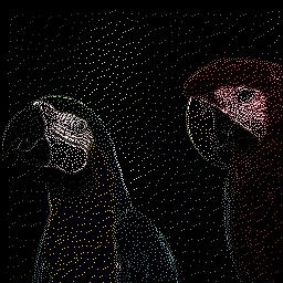
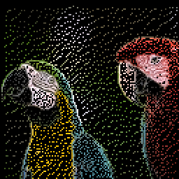
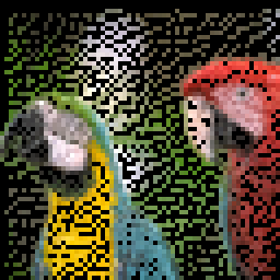
(a) ${\bf b}^{{\bf h}},I_{{\bf h}}^{{\bf H}}{\bf b}^{{\bf h}},\dots$ with normalisation

(b) ${\bf b}^{{\bf h}},I_{{\bf h}}^{{\bf H}}{\bf b}^{{\bf h}},\dots$ without normalisation

Figure 10: Restriction of the right-hand side ${\bf b}^{{\bf h}}$. The top row shows the restriction with the reweighting, the bottom row without. Without reweighting, the colours loose intensity on the coarser grids.

With these preparations, we state the full multigrid method as algorithm 5. It consists of nested iteration (cf. algorithm 4) for a good starting vector followed by several $\mu$-cycles (cf. algorithm 3). The $\mu$-cycle for $\mu=1$ is also called $V$-cycle and the $\mu$-cycle with $\mu=2$ is also called $W$-cycle.

Algorithm 3 $\mu$-cycle (${\bf v}^{\bf h}={\tt MG}({\bf v}^{\bf h},{\bf b}^{\bf h})$)

  if $\Omega^{\bf h}=$ coarsest grid then

     solve $B^{\bf h}{\bf v}^{\bf h}={\bf b}^{\bf h}$ by direct solver

  else

     relax $\nu_{1}$ times $B^{\bf h}{\bf u}^{\bf h}={\bf b}^{\bf h}$ with given starting value ${\bf v}^{\bf h}$

     ${\bf r}^{\bf H}=(\overrightarrow{{\bf 1}}-{\bf c}^{\bf H})\circ I_{\bf h}^{\bf H}({\bf b}^{\bf h}-B^{\bf h}{\bf v}^{\bf h})$

     ${\bf v}^{\bf H}=0$

     ${\bf v}^{\bf H}={\tt MG}({\bf v}^{\bf H},{\bf r}^{\bf H})$ $\mu$ times

     correct ${\bf v}^{\bf h}={\bf v}^{\bf h}+I_{\bf H}^{\bf h}{\bf v}^{\bf H}$

     relax $\nu_{2}$ times $B^{\bf h}{\bf u}^{\bf h}={\bf b}^{\bf h}$ with starting value ${\bf v}^{\bf h}$

  end if

Algorithm 4 Nested iteration (${\bf v}^{\bf h}={\tt NI}({\bf b}^{\bf h})$)

  if $\Omega^{\bf h}=$ coarsest grid then

     solve $B^{\bf h}{\bf v}^{\bf h}={\bf b}^{\bf h}$ by direct solver

  else

     ${\bf b}^{\bf H}=(I_{\bf h}^{\bf H}({\bf c}^{\bf h}\circ{\bf b}^{\bf h})\oslash(I_{\bf h}^{\bf H}{\bf c}^{\bf h})$

  end if

  ${\bf v}^{\bf H}={\tt NI}({\bf b}^{\bf H})$

  prolongate ${\bf v}^{\bf h}=I_{\bf H}^{\bf h}{\bf v}^{\bf H}$${\bf v}^{\bf h}={\tt MG}({\bf v}^{\bf h},{\bf b}^{\bf h})$ $\nu_{0}$ times

Algorithm 5 Full multigrid (${\bf v}^{\bf h}={\tt FMG}({\bf v}^{\bf h},{\bf b}^{\bf h})$)

   ${\bf v}^{\bf h}={\tt NI}({\bf b}^{\bf h})$${\bf v}^{\bf h}={\tt MG}({\bf v}^{\bf h},{\bf b}^{\bf h})$ $k$ times

6 Numerical experiments

In this section, we present some experiments with our decoding scheme. In the first subsection, we show that the new method outperforms standard time-integration methods. That the method compares to other (linear) edge-compressing schemes is shown in the second subsection. Finally, we demonstrate the use of our scheme on a real-world device.

6.1 Performance of the integrator

Basically, we have to compute the solution ${\bf y}(t)$ of the system of ordinary differential equations (1) for a large time $t$. After subdividing the interval $[0,t]$ in $n$ subintervals, the standard and most-used methods to approximate this solution are the implicit (or backward) Euler method

$${\bf y}(t)\approx\left(\gamma(\gamma I-A)^{-1}\right)^{n}{\bf b}_{0},\quad\gamma=\frac{n}{t}\,$$ (7)

and the Crank–Nicolson method

$${\bf y}(t)\approx\left((\gamma I+A)(\gamma I-A)^{-1}\right)^{n}{\bf b},\quad\gamma=\frac{2n}{t}\,.$$ (8)

The larger $n$, the more accurate is the approximation. To apply both methods, we have so solve $n$ linear systems of exactly the same type as for the Krylov method. Since this is the largest workload, we compare the methods with respect to the number of necessary solutions of linear systems of this type. For our edge-compressed all-white square test picture of section 4, the relative error in the Euclidean norm is shown in figure 11. For $t=10$, $t=10^{2}$, $t=10^{3}$, and $t=10^{4}$, the error of the methods versus the number of necessary solutions of the large linear system are shown. For larger $t$, the Crank-Nicolson method becomes worse, (which is a known behaviour due to stability considerations), while the backward Euler scheme remains unaffected. For large $t$ and an approximation error of about $10^{-3}$, the implicit Euler scheme needs to solve $1000$ linear systems of the type $(\gamma I-A){\bf x}={\bf b}$, while the Krylov method only needs $8$. This is a factor of $125$ times faster. This clearly demonstrates our main contribution that the Krylov method can solve homogeneous inpainting problems with a significantly improved speed.

Figure 11: Error of the implicit Euler scheme (red) diamond-marked line, error of the Crank-Nicolson method (orange) square-marked line, and the rational Krylov subspace method with optimal gamma (green) solid line versus number of linear system solves for $t=10$ on the top left-hand side, $t=10^{2}$ on the top right-hand side, $t=10^{3}$ on the bottom left-hand side, $t=10^{4}$ on the bottom right-hand side.

6.2 Quality of compression

In order to ensure that decoding the edge-compressed pictures by the Krylov method does not affect the quality of the recovered image, we provide experiments with pictures of the Kodak lossless true colour image suite (cf. Kodak ), whose thumbnail pictures can be seen in figure 12.

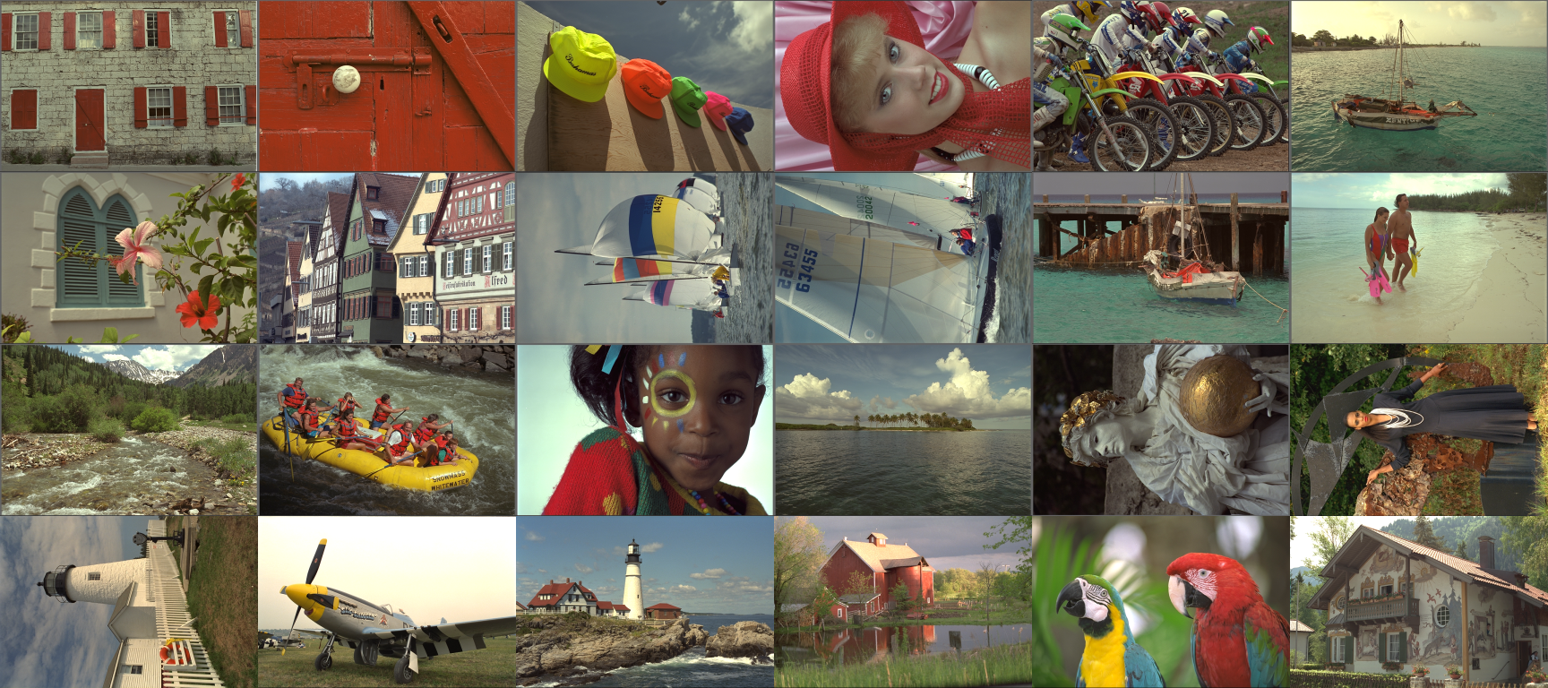
Figure 12: Kodak image suite Kodak , running from image kodim01 (top left) to image kodim24 (bottom right).

In order to measure the deviation of the decoded compressed picture from the original picture, we use the mean-square error (MSE). For two colour pictures ${\bf u},{\bf v}\in\mathbb{R}^{M,N,3}$ with three colour channels and dimension $M\times N$, the mean-square error is given as

$$\operatorname{MSE}({\bf u},{\bf v})\coloneqq\frac{1}{3MN}\sum_{k=1}^{3}\sum_{i=1}^{M}\sum_{j=1}^{N}(u_{i,j,k}-v_{i,j,k})^{2}.$$

We use $\mu=2$ in algorithm 3, which corresponds to the W-cycle, and $4$ pre- as well as post-relaxation steps. For the nested iteration in order to obtain a good starting value, we use $\nu_{0}=1$ in algorithm 4. For these pictures, we use $7$ levels in the multigrid method.

We found that for a large time $t=10^{7}$, the extended Krylov subspace with dimension $m=3$ is sufficient to approximate the steady state. This means that only one solve of a linear system with the multigrid method is necessary. For the optimal $\gamma=1.5/t$ and picture kodim07 of the test suite, the steady state and the reconstruction can be seen on the bottom of figure 13 on the left-hand and right-hand side, respectively. On the top of figure 13 on the left-hand side, the original picture is shown for comparison.

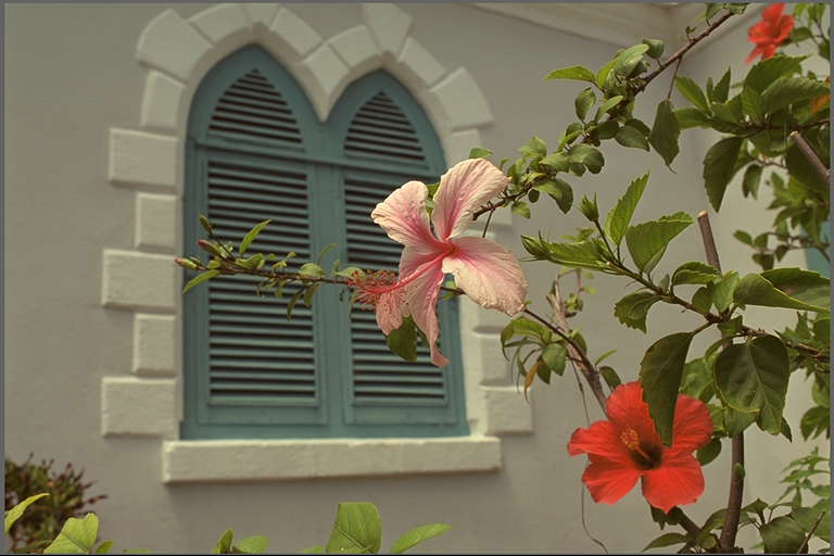
(a) original image

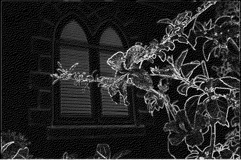
(b) inpainting mask

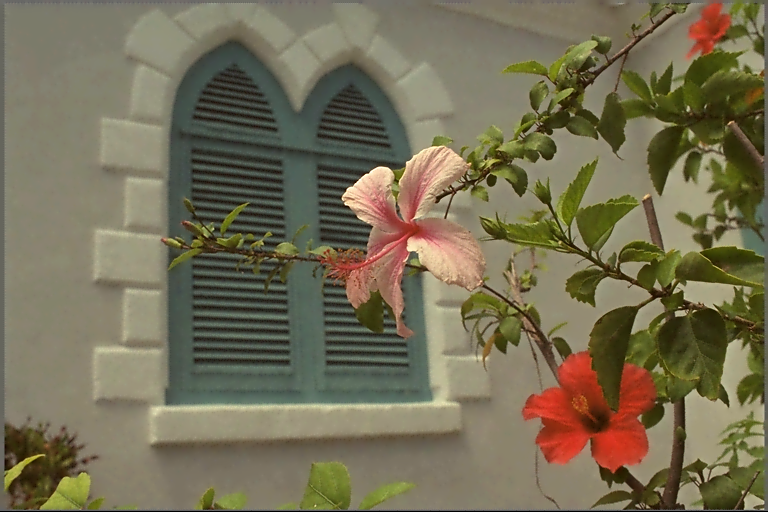
(c) steady state

(d) reconstruction, $t=10^{7}$

Figure 13: (a) shows the original image and (b) the dithering-based inpainting mask. (c) is the steady state of the heat equation and (d) shows the reconstruction by computing the solution of the heat equation up to time $t=10^{7}$.

The image has been compressed by the dithering-based method. The mask can be seen on the top of figure 13 on the right-hand side. A closer inspection reveals that the difference between the steady state and the reconstruction with a large time is several orders of magnitude smaller than the difference of both with respect to the original. The same observation turned out to be true for the whole test set and for dithering-based as well as the edge-based compression of the images. We present the results in table 2. Here, we also state the peak signal-to-noise ratio (PSNR),

$$\operatorname{PSNR}({\bf u},{\bf v})\coloneqq 10\cdot\log_{10}\left(\frac{255^{2}}{\operatorname{MSE}({\bf u},{\bf v})}\right)[$\mathrm{dB}$],$$

which is the most commonly used measure for the quality of reconstructions in lossy compression schemes. We also state the compression rate in bits per pixels (bpp) which refers to the average number of bits needed to encode each image pixel. The original pictures are RGB pictures using $8$ bits per colour channel which gives $24$ bpp in the original pictures. Better values are marked in bold. The averages (avg) over all values are shown in the last row.

Table 2: Comparison of the quality of the reconstruction for the proposed decoding scheme for dithering-based as well as edge-based compressed images of the test suite.

img	dithering-based			edge-based
	bpp	MSE	PSNR	bpp	MSE	PSNR
01	2.37	161.42	26.05	2.17	164.39	25.97
02	2.23	26.63	33.88	1.99	64.59	30.03
03	2.18	14.23	36.60	1.66	50.11	31.13
04	2.37	26.31	33.93	2.11	47.98	31.32
05	2.74	144.67	26.53	2.43	165.88	25.93
06	2.34	86.72	28.75	2.00	148.47	26.41
07	2.38	22.65	34.58	1.45	62.19	30.19
08	2.68	271.95	23.79	1.99	282.04	23.63
09	2.16	20.77	34.96	1.19	51.70	31.00
10	2.22	22.90	34.53	1.61	46.91	31.42
11	2.41	53.89	30.82	2.06	86.52	28.76
12	2.13	20.24	35.07	1.77	39.67	32.15
13	2.70	261.84	23.95	2.99	286.27	23.56
14	2.63	77.51	29.24	2.50	101.81	28.05
15	2.34	26.98	33.82	1.86	74.44	29.41
16	2.09	35.29	32.65	1.81	63.26	30.12
17	2.28	22.83	34.55	1.92	53.52	30.85
18	2.71	74.10	29.43	2.57	120.92	27.31
19	2.30	52.76	30.91	1.70	106.74	27.85
20	2.05	22.22	34.66	1.28	68.80	29.76
21	2.36	49.72	31.17	1.72	111.10	27.67
22	2.59	42.20	31.88	2.42	72.10	29.55
23	2.36	9.86	38.19	1.88	39.84	32.13
24	2.57	102.71	28.01	2.18	153.04	26.28
avg	2.38	68.77	31.58	1.97	102.60	28.77

The results in table 2 show that the decoding method is sufficiently accurate and not worse than a scheme that directly computes the steady state. The direct computation of the steady state leads to a table with only very minor variations in the numbers.

6.3 Performance on an everyday device

High compression rates are particularly important for embedded devices like smartphones, smart TV sets, and smart watches where storage is limited. Nowadays, these devices include embedded GPUs (Graphics Processing Unit) which allow to accelerate image processing tasks, considerably. The industry standard to accelerate graphics by the use of these GPUs is OpenGL ES (Open Graphics Library for Embedded Systems) managed by the non-profit Khronos group (cf. khronos ). For our experiment, we will use the version OpenGL ES 3.2, which is available on $73.50\%$ of the devices as of the 31st July 2021 (cf. OpenGLdistro ) as well as the version OpenGL ES 3.1 with the extension GL_EXT_color_buffer_float which allows to render to float textures attached to a framebuffer. Our approach, with the implementation details given in section 5, perfectly fits to the OpenGL application interface. Pictures are treated as textures that are operated on in a parallel manner by the use of vertex and fragment shaders. Turning the matrices in sparse formats would not lead to algorithms that can be easily ported to embedded GPUs. We first used a desktop computer with a NVIDIA GeForce GT 730/PCIe/SSE2. OpenGL ES 3.2 is available on this GPU. The average time of ten runs of our program to decode the $512\times 512$ RGB picture in the middle of figure 1 to the picture on the right-hand side of figure 1 was $0.116\,s$.The dimension of system (1) is $786432$ for this picture. On a notebook with the integrated graphics processor Intel(R) HD Graphics 620 (KBL GT2), the average time of ten runs was $0.049\,s$. OpenGL ES 3.2 is also available on this graphics processor. As an embedded device, we used smartphone running Android version 9 (pie) with a Qualcomm Adreno $308$ GPU with the same picture. This phone allows for version OpenGL ES 3.1 with GL_EXT_color_buffer_float extension. The C code was compiled with the native development toolkit for Android systems (cf. AndroidNDK ). The transition from the top of figure 14

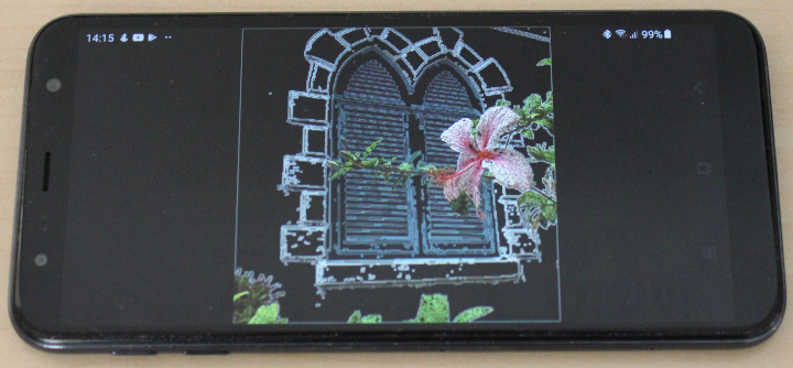
(a) compression

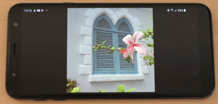
(b) reconstruction

Figure 14: Experiment on a smartphone

to the bottom of figure 14 took about $0.718\,s$ in average. With less than a second, this seems to be fast enough to decode edge-compressed pictures stored on this phone in a real-life application. On a high-end smartphone with a more powerful GPU, the decoding is expected to be faster.

7 Conclusion

We presented an efficient method to solve inpainting problems by homogeneous diffusion based on extended Krylov subspaces. The method is basically applicable to all inpainting problems of this type. We studied the problem of decoding edge-based and dithering-based compressed images, where the boundaries for the inpainting problems are especially challenging. To our best knowledge, no other method is known that can provably solve inpainting problems up to a large time $t$ with such an accuracy and efficiency.

References

• (1) Al-Mohy, A.H., Higham, N.J.: Computing the action of the matrix exponential, with an application to exponential integrators. SIAM J. Sci. Comput. 33(2), 488–511 (2011). https://doi.org/10.1137/100788860
• (2) Andersson, J.E.: Approximation of $e^{-x}$ by rational functions with concentrated negative poles. J. Approx. Theory 32(2), 85–95 (1981). https://doi.org/10.1016/0021-9045(81)90106-4
• (3) Android Developers: Android NDK (accessed 9 September 2020). https://developer.android.com/ndk
• (4) Android Developers: Distribution dashbord (accessed 9 September 2021). https://developer.android.com/about/dashboards/index.html#OpenGL
• (5) Beckermann, B., Güttel, S.: Superlinear convergence of the rational Arnoldi method for the approximation of matrix functions. Numer. Math. 121(2), 205–236 (2012). https://doi.org/10.1007/s00211-011-0434-8
• (6) Belhachmi, Z., Bucur, D., Burgeth, B., Weickert, J.: How to choose interpolation data in images. SIAM J. Appl. Math. 70(1), 333–352 (2009). https://doi.org/10.1137/080716396
• (7) Brezinski, C., Novati, P., Redivo-Zaglia, M.: A rational Arnoldi approach for ill-conditioned linear systems. J. Comput. Appl. Math. 236(8), 2063–2077 (2012). https://doi.org/10.1016/j.cam.2011.09.032
• (8) Bruhn, A., Weickert, J., Feddern, C., Kohlberger, T., Schnörr, C.: Variational optic flow computation in real-time. IEEE Transactions on Image Processing 14(5), 608–615 (2005). https://doi.org/10.1109/TIP.2005.846018
• (9) Buccini, A., Donatelli, M., Reichel, L.: Iterated Tikhonov regularization with a general penalty term. Numer. Linear Algebra Appl. 24(4), e2089, 12 (2017). https://doi.org/10.1002/nla.2089
• (10) Canny, J.: A Computational Approach of Edge Detection. IEEE Transactions on Pattern Analysis and Machine Intelligence PAMI-8(6), 679–698 (1986)
• (11) Carlsson, S.: Sketch based coding of grey level images. Signal Processing 15(1), 57–83 (1988). https://doi.org/10.1016/0165-1684(88)90028-X
• (12) Druskin, V., Knizhnerman, L.: Extended Krylov subspaces: approximation of the matrix square root and related functions. SIAM J. Matrix Anal. Appl. 19(3), 755–771 (1998). http://dx.doi.org/10.1137/S0895479895292400
• (13) Elder, J.H.: Are edges incomplete? International Journal of Computer Vision 34, 97–122 (1999). https://doi.org/10.1023/A:1008183703117
• (14) van den Eshof, J., Hochbruck, M.: Preconditioning Lanczos approximations to the matrix exponential. SIAM J. Sci. Comp. 27(4), 1438–1457 (2006). https://doi.org/10.1137/040605461
• (15) Floyd, R.W., Steinberg, L.: An adaptive algorithm for spatial grey scale. Proceedings of the Society of Information Display 17, 75–77 (1976)
• (16) Franzen, R.: Kodak Lossless True Color Image Suite. http://r0k.us/graphics/kodak. Accessed: 2020-03-22
• (17) Göckler, T., Grimm, V.: Convergence Analysis of an Extended Krylov Subspace Method for the Approximation of Operator Functions in Exponential Integrators. SIAM J. Numer. Anal. 51(4), 2189–2213 (2013). http://dx.doi.org/10.1137/12089226X
• (18) Göckler, T., Grimm, V.: Uniform approximation of $\varphi$-functions in exponential integrators by a rational Krylov subspace method with simple poles. SIAM J. Matrix Anal. Appl. 35(4), 1467–1489 (2014). http://dx.doi.org/10.1137/140964655
• (19) Grimm, V.: Resolvent Krylov subspace approximation to operator functions. BIT Numerical Mathematics 52(3), 639–659 (2012). https://doi.org/10.1007/s10543-011-0367-8
• (20) Grimm, V.: A conjugate-gradient-type rational Krylov subspace method for ill-posed problems. Inverse Problems 36(1), 015008, 19 (2020). https://doi.org/10.1088/1361-6420/ab5819
• (21) Grimm, V., Göckler, T.: Automatic smoothness detection of the resolvent Krylov subspace method for the approximation of $C_{0}$-semigroups. SIAM J. Numer. Anal. 55(3), 1483–1504 (2017). https://doi.org/10.1137/15M104880X
• (22) Higham, N.J.: Functions of matrices. Society for Industrial and Applied Mathematics (SIAM), Philadelphia, PA (2008). https://doi.org/10.1137/1.9780898717778
• (23) Hochbruck, M., Ostermann, A.: Exponential integrators. Acta Numer. 19, 209–286 (2010). https://doi.org/10.1017/S0962492910000048
• (24) Hoeltgen, L., Setzer, S., Weickert, J.: An optimal control approach to find sparse data for laplace interpolation. In: A. Heyden, F. Kahl, C. Olsson, M. Oskarsson, X.C. Tai (eds.) Energy Minimization Methods in Computer Vision and Pattern Recognition. Lecture notes in Computer Science, vol. 8081, pp. 151–164. Springer, Berlin (2013). https://doi.org/10.1007/978-3-642-40395-8_12
• (25) Hummel, R., Moniot, R.: Reconstructions from zero-crossings in scale space. IEEE Transactions on Acoustics, Speech and Signal Processing 37, 2111–2130 (1989). https://doi.org/10.1109/29.45555
• (26) The Khronos Group Inc.: Khronos Group (2021, (accessed 9 September 2020)). https://www.khronos.org/
• (27) Knizhnerman, L., Simoncini, V.: A new investigation of the extended Krylov subspace method for matrix function evaluations. Numer. Linear Algebra Appl. 17(4), 615–638 (2010). https://doi.org/10.1002/nla.652
• (28) Mainberger, M., Bruhn, A., Weickert, J., Forchhammer, S.: Edge-based compression of cartoon-like images with homogeneous diffusion. Pattern Recognition 44(9), 1859–1873 (2011). https://doi.org/10.1016/j.patcog.2010.08.004
• (29) Mainberger, M., Hoffmann, S., Weickert, J., Tang, C.H., Johannsen, D., Neumann, F., Doerr, B.: Optimising spatial and tonal data for homogeneous diffusion inpainting. In: A.M. Bruckstein, B.M. ter Haar Romney, A.M. Bronstein, M.M. Bronstein (eds.) Scale Space and Variational Methods in Computer Vision. SSVM 2011. Lecture Notes in Computer Science, vol. 6667, pp. 27–37. Springer, Berlin, Heidelberg (2012). https://doi.org/10.1007/978-3-642-24785-9_3
• (30) Marr, D.: Early processing of visual information. Philosophical Transactions of the Royal Society of London. Series B, Biological Sciences 275(942), 483–519 (1975). https://doi.org/10.1098/rstb.1976.0090
• (31) Marr, D., Hildreth, E.: Theory of edge detection. Proceedings of the Royal Society of London B 207, 187–217 (1980)
• (32) Ramlau, R., Reichel, L.: Error estimates for Arnoldi-Tikhonov regularization for ill-posed operator equations. Inverse Problems 35(5), 055002, 23 (2019). https://doi.org/10.1088/1361-6420/ab0663
• (33) Reid, M.M., Millar, R.J., Black, N.D.: Second-generation image coding: an overview. ACM Computing Surveys 29, 3–29 (1997). https://doi.org/10.1145/248621.248622
• (34) Ruhe, A.: Rational Krylov sequence methods for eigenvalue computation. Linear Algebra Appl. 58, 391–405 (1984). https://doi.org/10.1016/0024-3795(84)90221-0
• (35) Ruhe, A.: Rational Krylov: A practical algorithm for large sparse nonsymetric matrix pencils. SIAM J. Sci. Comput. 19, 1535–1551 (1998). https://doi.org/10.1137/S1064827595285597
• (36) Saad, Y.: Iterative methods for sparse linear systems, second edn. Society for Industrial and Applied Mathematics, Philadelphia, PA (2003). https://doi.org/10.1137/1.9780898718003
• (37) Schönlieb, C.B.: Partial differential equation methods for image inpainting, Cambridge Monographs on Applied and Computational Mathematics, vol. 29. Cambridge University Press, New York (2015). https://doi.org/10.1017/CBO9780511734304
• (38) Zeevi, Y., Rotem, D.: Image reconstruction from zero-crossings. IEEE Transactions on Acoustics, Speech and Signal Processing 34, 1269–1277 (1986). https://doi.org/10.1109/TASSP.1986.1164922