The Fragility of Optimized Bandit Algorithms

The Fragility of Optimized Bandit Algorithms

Lin Fan Department of Management Science and Engineering, Stanford University, Stanford, CA 94305, linfan@stanford.edu Peter W. Glynn Department of Management Science and Engineering, Stanford University, Stanford, CA 94305, glynn@stanford.edu

Much of the literature on optimal design of bandit algorithms is based on minimization of expected regret. It is well known that algorithms that are optimal over certain exponential families can achieve expected regret that grows logarithmically in the number of trials, at a rate specified by the Lai-Robbins lower bound. In this paper, we show that when one uses such optimized algorithms, the resulting regret distribution necessarily has a very heavy tail, specifically, that of a truncated Cauchy distribution. Furthermore, for $p>1$, the $p$’th moment of the regret distribution grows much faster than poly-logarithmically, in particular as a power of the total number of trials. We show that optimized UCB algorithms are also fragile in an additional sense, namely when the problem is even slightly mis-specified, the regret can grow much faster than the conventional theory suggests. Our arguments are based on standard change-of-measure ideas, and indicate that the most likely way that regret becomes larger than expected is when the optimal arm returns below-average rewards in the first few arm plays, thereby causing the algorithm to believe that the arm is sub-optimal. To alleviate the fragility issues exposed, we show that UCB algorithms can be modified so as to ensure a desired degree of robustness to mis-specification. In doing so, we also show a sharp trade-off between the amount of UCB exploration and the tail exponent of the resulting regret distribution.

Multi-armed Bandits, Regret Distribution, Limit Theorems, Mis-specification, Robustness Manuscript version – May 24, 2023

1 Introduction

The multi-armed bandit (MAB) problem is a widely studied model that is both useful in practical applications and is a valuable theoretical paradigm exhibiting the exploration-exploitation trade-off that arises in sequential decision-making under uncertainty. More specifically, the goal in a MAB problem is to maximize the expected reward derived from playing, at each time step, one of $K$ bandit arms. Each arm has its own unknown reward distribution, so that playing a particular arm both provides information about that arm’s reward distribution (exploration) and provides an associated random reward (exploitation). One measure of the quality of a MAB algorithm is the (pseudo-)regret $R(T)$, which is essentially the number of times the sub-optimal arms are played over a time horizon $T$, as compared to an oracle that acts optimally with knowledge of the means of all arm reward distributions; a precise definition will be given in Section 2.

There is an enormous literature on this problem, with much of the research having been focused on algorithms that attempt to minimize expected regret. In this regard, a fundamental result is the Lai-Robbins lower bound that establishes that the expected regret $\mathbb{E}[R(T)]$ grows logarithmically in $T$, with a multiplier that depends on the Kullback-Leibler (KL) divergences between the optimal arm and each of the sub-optimal arms; see Lai and Robbins (1985). A predominant focus in the bandit literature is on designing algorithms that attain the Lai-Robbins lower bound over particular exponential families of distributions; see Lai and Robbins (1985) and Burnetas and Katehakis (1996). We call such algorithms optimized. Among the many optimized algorithms in the literature, two prominent examples are the KL-upper confidence bound (KL-UCB) algorithm and Thompson sampling (TS); see Cappé et al. (2013) (and earlier work: Garivier and Cappé (2011), Maillard et al. (2011)) for KL-UCB, and Korda et al. (2013) for TS (originally proposed by Thompson (1933)). (Earlier optimized UCB-type algorithms can be found in, for example, Lai (1987) and Agrawal (1995).)

In this paper, we show that any such optimized algorithm necessarily has the undesirable property that the tail of $R(T)$ is very heavy. In particular, because $\mathbb{E}[R(T)]$ is $O(\log(T))$ (where $O(a_{T})$ is any sequence having the property that its absolute value is dominated by a constant multiple of $a_{T}$), Markov’s inequality implies that for $c>0$, $\mathbb{P}(R(T)>cT)=O(\log(T)/T)$ as $T\to\infty$. One of our central results is a lower bound characterization of $\mathbb{P}(R(T)>cT)$ that roughly establishes that this probability is attained, namely it is roughly of order $T^{-1}$ for optimized algorithms. More precisely, our Theorem 3.2 shows that optimized MAB algorithms automatically have the property that

$$\mathbb{P}(R(T)>x)\asymp\frac{1}{x}$$

as $T\to\infty$, uniformly in $x$ with $T^{a}\leq x\leq cT$, for any $0<a<1$ and suitable $c>0$. (We write $a_{T}\asymp b_{T}$ as $T\to\infty$ whenever $\log(a_{T})/\log(b_{T})$ converges to $1$ as $T\rightarrow\infty$.) In other words, the tail of the regret $R(T)$ looks, in logarithmic scale, like that of a truncated Cauchy distribution (truncated due to the time horizon $T$). Thus, such algorithms fail to produce logarithmic regret with large probability, and when they fail to produce such regret, the magnitude of the regret can be very large. This is one sense in which bandit algorithms optimized for expected regret can be fragile.

An additional sense in which such optimized bandit algorithms are fragile is their sensitivity to model mis-specification. By this, we mean that if an algorithm has been optimized to attain the Lai-Robbins lower bound over a particular class of bandit environments (e.g., with the arm distributions belonging to a specific exponential family), then we can see much worse regret behavior when the environment presented to the algorithm does not belong to the class. For example, we show that for the KL-UCB algorithm designed for Gaussian environments with known and equal variances but unknown means, the expected regret for Gaussian environments can grow as a power $T^{r}$ when the variance of the optimal arm’s rewards is larger than the variance built into the algorithm’s design. In fact, $r$ can be made arbitrarily close to $1$ depending on how large the optimal arm’s variance is, relative to the variance of the algorithm’s design (Corollary 4.2). In other words, even when the mis-specification remains Gaussian, the expected regret can grow at a rate close to linear in the time horizon $T$. Besides mis-specification of the bandits’ marginal reward distributions, optimized algorithms are equally susceptible to mis-specification of the serial dependence structure of rewards. For example, expected regret deteriorates similarly as reward processes (e.g., evolving as Markov chains) become more autocorrelated (Corollary 4.7, Corollary 4.8 and Example 4.9).

A final sense in which such optimized algorithms are fragile is that when one only slightly modifies the objective, the regret behavior of the algorithm can look much worse. In particular, suppose that we consider minimizing $\mathbb{E}[R(T)^{p}]$ for some $p>1$, rather than $\mathbb{E}[R(T)]$. This objective would arise naturally, for example, in the presence of risk aversion to high regret. One might reasonably expect that algorithms optimized for $\mathbb{E}[R(T)]$ would have the property that $\mathbb{E}[R(T)^{p}]$ would then grow poly-logarithmically in $T$. However, the Cauchy-type tails discussed earlier imply that $(R(T)/\log(T))^{p}$ is not a uniformly integrable sequence. We show in Corollary 4.10 that for optimized algorithms, $\mathbb{E}[R(T)^{p}]$ grows roughly at least as fast as $T^{p-1}$ as $T\to\infty$.

Our proofs rely on change-of-measure arguments that also provide insight into how algorithms optimized for expected regret can fail to identify the optimal arm, thereby generating large regret. For example, we show that conditional on large regret, the sample means of sub-optimal arms obey laws of large numbers that indicate that they continue to behave in their usual way; see Proposition 3.13. This suggests that the most likely way that large regret occurs for such optimized algorithms is when the optimal arm under-performs in the exploration phase at the start of the experiment, after which it is played infrequently, thereby generating large amounts of regret. This intuitive scenario has been heuristically considered several times in the literature (see, e.g., Audibert et al. (2009)), but this paper provides the theoretical justification for its central role in generating large regret.

To mitigate some of the fragility issues we expose, we show how to modify UCB algorithms so as to ensure a desired degree of robustness to model mis-specification. The modification is designed to lighten the regret distribution tail to a given exponent, thereby creating a prescribed margin of safety against model mis-specification. As a part of our analysis, we provide a trade-off between the logarithmic rate of exploration and the resulting heaviness of the regret tail. For example, in well-specified settings, if one increases the amount of exploration by a factor of $(1+b)$ times for any desired $b>0$, then the tail of the resulting regret distribution will have an exponent of $-(1+b)$ (or less). In particular, $\mathbb{P}(R(T)>x)\asymp x^{-(1+b)}$ as $T\to\infty$, uniformly in $x$ with $\log^{a}(T)\leq x\leq cT$, for any $a>1$ and suitable $c>0$.

The rest of the paper is structured as follows. After discussing related work in Section 1.1, we introduce the setup for the rest of the paper in Section 2. In Section 3.1, we establish our main result, Theorem 3.2, that optimized algorithms have regret distributions for which the tails are truncated Cauchy. This result requires a technical condition (Definition 3.1), which holds essentially for all continuous reward distributions. To illustrate the key ideas behind Theorem 3.2, we prove a simplified version of the result in Section 3.2. We develop in Section 3.3 tight upper bounds characterizing the regret tail for KL-UCB in settings where the regret tail is lighter than truncated Cauchy (because the condition in Definition 3.1 does not hold); see Theorem 3.14. In Section 3.4, we provide an alternative, intuitive proof of the generalized Lai-Robbins lower bound for expected regret (Theorem 3.16) by focusing on the regret tail and using our change-of-measure arguments. Our proof sheds new light on the result and further provides a sharp trade-off between lighter regret tails and larger expected regret (Proposition 3.21). In Sections 4.1 and 4.3, we show that the performance of optimized algorithms can deteriorate sharply under the slightest amount of mis-specification of the distribution or the serial dependence structure of the rewards. These insights make use of results from Section 4.2, where we establish general lower bounds for the regret tail of algorithms such as KL-UCB when the rewards come from stochastic processes (Theorem 4.5). Moreover, we show in Section 4.4 that such optimized algorithms offer no control over the $p$’th moment of regret for any $p>1$. In Section 5.1, building upon Section 3.3, we discuss how to design UCB algorithms to achieve any desired exponent of the regret tail uniformly over a general class of bandit environments. We then discuss how lighter regret tails provide protection against mis-specification of the distribution of rewards and the serial dependence structure of rewards in Sections 5.2 and 5.3, respectively. In Section 7, we examine some numerical experiments. We conclude with the proofs of Theorems 3.2 and 3.14 in Sections 6.1 and 6.2, respectively.

1.1 Related Work

In terms of related work, Audibert et al. (2009), Salomon and Audibert (2011) study concentration properties of the regret distribution. In particular, Audibert et al. (2009) develop a finite-time upper bound on the tail of the regret distribution for a particular version of UCB in bounded reward settings. Their upper bound has polynomial rates of tail decay, which are adjustable depending on algorithm settings. One of their motivations for developing regret tail bounds is to establish a trade-off between the rate of exploration and the resulting heaviness of the regret tail. However, it is lower bounds on the regret tail that are needed to conclusively establish the trade-off and confirm that the regret distribution is heavy-tailed. Our lower bounds turn out to be frequently tight.

The regret distribution tail approximations developed in the current work are complementary to the strong laws of large numbers (SLLN’s) and central limit theorems (CLT’s) developed for bandit algorithms in instance-dependent settings in Fan and Glynn (2022). For example, in the Gaussian bandit setting (with unit variances for simplicity), for both TS and UCB, the regret satisfies the SLLN:

$$\frac{R(T)}{\log(T)}\overset{\text{a.s.}}{\to}\sum_{i\neq i^{*}}\frac{2}{\Delta_{i}}$$

and the CLT:

$$\frac{R(T)-\sum_{i\neq i^{*}}\frac{2}{\Delta_{i}}\log(T)}{\sqrt{\sum_{i\neq i^{*}}\frac{8}{\Delta_{i}^{2}}\log(T)}}\Rightarrow N(0,1),$$

where $\Delta_{i}>0$ is the difference between the mean of the optimal arm $i^{*}$ and that of sub-optimal arm $i$, and $\Rightarrow$ denotes convergence in distribution. These results can viewed as describing the typical behavior and fluctuation of regret when $T$ is large. This stands in contrast to the results in the current work, which describe the tail behavior of the regret. Tails are generally affected by atypical behavior. As noted above, our arguments show that the regret tail is impacted by trajectories on which the algorithm mis-identifies the optimal arm. The mean and the variance in the CLT both scale as $\log(T)$ with the time horizon $T$. By analogy with the large deviations theory for sums of iid random variables, this suggests that large deviations of regret correspond to deviations from the expected regret that are of order $\log(T)$. We characterize the tail of the regret beyond $\log^{1+\epsilon}(T)$ for small $\epsilon>0$, and we save the analysis of deviations on the $\log(T)$ scale for future work.

Recently, Ashutosh et al. (2021) show that for an algorithm to achieve expected regret of logarithmic order across a collection of bandit instances, the distributional class of arm rewards cannot be too large. For example, if the rewards are known to be sub-Gaussian, then an upper bound restriction on the variance proxy is required. They conclude that if such a restriction is mis-specified, then the worst case expected regret could be of polynomial order. Their result provides no information about algorithm behavior for any particular bandit instance, nor does it cover narrower classes of distributions (e.g., Gaussian).

There is also a growing literature on risk-averse formulations of the MAB problem, with a non-comprehensive list being: Sani et al. (2012), Maillard (2013), Zimin et al. (2014), Szorenyi et al. (2015), Vakili and Zhao (2016), Galichet et al. (2013), Cassel et al. (2018), Tamkin et al. (2019), Zhu and Tan (2020), Prashanth et al. (2020), Baudry et al. (2021), Khajonchotpanya et al. (2021). As noted earlier, risk-averse formulations involve defining arm optimality using criteria other than the expected reward. These papers consider mean/variance criteria, value-at-risk, or conditional value-at-risk measures, and develop algorithms which achieve good (or even optimal in some cases) regret performance relative to their chosen criterion. Our results serve as motivation for these papers, and highlight the need to consider robustness in many MAB problem settings.

2 Model and Preliminaries

2.1 The Multi-armed Bandit Framework

A $K$-armed MAB evolves within a bandit environment $\nu=(Q_{1},\dots,Q_{K})$, where each $Q_{i}$ is a distribution on $\mathbb{R}$. At time $t$, the decision-maker selects an arm $A(t)\in[K]:=\{1,\dots,K\}$ to play. The conditional distribution of $A(t)$ given $A(1),Y(1),\dots,A(t-1),Y(t-1)$ is $\pi_{t}(\cdot\mid A(1),Y(1),\dots,A(t-1),Y(t-1))$, where $\pi=(\pi_{t},t\geq 1)$ is a sequence of probability kernels, which constitutes the bandit algorithm (with $\pi_{t}$ defined on $([K]\times\mathbb{R})^{t}\times 2^{[K]}$). Upon selecting the arm $A(t)$, a reward $Y(t)$ from arm $A(t)$ is received as feedback. The conditional distribution of $Y(t)$ given $A(1),Y(1),\dots,A(t-1),Y(t-1),A(t)$ is $Q_{A(t)}(\cdot)$. We write $X_{i}(t)$ to denote the reward received when arm $i$ is played for the $t$-th instance, so that $Y(t)=X_{A(t)}(N_{A(t)}(t))$, where $N_{i}(t)=\sum_{s=1}^{t}\mathbb{I}\left({A(s)=i}\right)$ denotes the number of plays of arm $i$ up to and including time $t$.

For any time $t$, the interaction between the algorithm $\pi$ and the environment $\nu$ induces a unique probability $\mathbb{P}_{\nu\pi}(\cdot)$ on $([K]\times\mathbb{R})^{\infty}$ for which

$$\mathbb{P}_{\nu\pi}(A(1)=a_{1},Y(1)\in dy_{1},\dots,A(t)=a_{t},Y(t)\in dy_{t})=\prod_{s=1}^{t}\pi_{s}(a_{s}\;|\;a_{1},y_{1},\dots,a_{s-1},y_{s-1})Q_{a_{s}}(dy_{s}).$$

For $t\geq 1$, we write $\mathbb{E}_{\nu\pi}[\cdot]$ to denote the expectation associated with $\mathbb{P}_{\nu\pi}(\cdot)$.

The quality of an algorithm $\pi$ operating in an environment $\nu=(Q_{1},\dots,Q_{K})$ is measured by the (pseudo-)regret (at time $T$):

$$R(T)=\sum_{i=1}^{K}N_{i}(T)\Delta_{i},$$

where $\Delta_{i}=\mu_{*}(\nu)-\mu(Q_{i})$ and $\mu_{*}(\nu)=\max_{Q\in\nu}\mu(Q)$. (For any distribution $Q$, we use $\mu(Q)$ to denote its mean.) An arm $i$ is called optimal if $\Delta_{i}=0$, and sub-optimal if $\Delta_{i}>0$. The goal in most settings is to find an algorithm $\pi$ which minimizes the expected regret $\mathbb{E}_{\nu\pi}[R(T)]$, i.e., plays the optimal arm(s) as often as possible in expectation.

When discussing the regret distribution tail in multi-armed settings, we will often reference (for any given environment) the $i$-th-best arm (with the $i$-th largest mean). For each $i=1,\dots,K$, we will use $r(i)\in[K]$ to denote the index/label of the $i$-th-best arm. To keep our discussions and derivations streamlined, unless specified otherwise, throughout the paper we will only consider environments where for each $i=1,\dots,K$, the $i$-th-best arm is unique.

2.2 Optimized Algorithms

In order to discuss optimized algorithms, we consider arm reward distributions from a one-dimensional exponential family, parameterized by mean, of the form:

$$P^{z}(dx)=\exp\bigl{(}\theta_{P}(z)\cdot x-\Lambda_{P}(\theta_{P}(z))\bigr{)}P(dx),\quad z\in\mathcal{I}_{P}.$$ (1)

Here, $P$ is a base distribution with cumulant generating function (CGF) $\Lambda_{P}$. We use $\mathcal{I}_{P}$ to denote the set of all possible means for distributions $P^{z}$ of the form in (1), with $\theta_{P}(z)$ being any real number in the set $\Theta_{P}=\{\theta\in\mathbb{R}:\Lambda_{P}(\theta)<\infty\}$. Moreover, for each $z\in\mathcal{I}_{P}$, we use $\theta_{P}(z)$ to denote the unique value for which $\mu(P^{z})=z$. (Also recall that $\Lambda_{P}^{\prime}(\theta_{P}(z))=z$.) Throughout the paper, we will always work with base distributions $P$ such that $\Theta_{P}$ contains a neighborhood of zero. For a base distribution $P$, we denote the mean-parameterized model in (1) via:

$$\mathcal{M}_{P}=\left\{P^{z}:z\in\mathcal{I}_{P}\right\},$$ (2)

which induces a class $\mathcal{M}_{P}^{K}$ of $K$-armed bandit environments, where each environment consists of a $K$-tuple of distributions from $\mathcal{M}_{P}$. The KL divergence between distributions in $\mathcal{M}_{P}$ with means $z_{1},z_{2}\in\mathcal{I}_{P}$ is denoted by $d_{P}(z_{1},z_{2})$, and can be expressed as:

$$d_{P}(z_{1},z_{2}) =\int\log\frac{dP^{z_{1}}}{dP^{z_{2}}}(x)\;P^{z_{1}}(dx)$$

$$=\Lambda_{P}(\theta_{P}(z_{2}))-\Lambda_{P}(\theta_{P}(z_{1}))-\Lambda_{P}^{\prime}(\theta_{P}(z_{1}))\cdot\bigl{(}\theta_{P}(z_{2})-\theta_{P}(z_{1})\bigr{)},$$ (3)

where $dP^{z_{1}}/dP^{z_{2}}$ denotes the likelihood ratio of $P^{z_{1}}$ to $P^{z_{2}}$.

From the seminal work of Lai and Robbins (1985), there is a precise characterization of the minimum possible growth rate of expected regret for an algorithm $\pi$ designed for $\mathcal{M}_{P}^{K}$, which is stated as follows. Let $\pi$ be (so-called) $\mathcal{M}_{P}$-consistent, satisfying for any $a>0$, any environment $\nu\in\mathcal{M}_{P}^{K}$, and each sub-optimal arm $i$:

$$\lim_{T\to\infty}\frac{\mathbb{E}_{\nu\pi}[N_{i}(T)]}{T^{a}}=0.$$ (4)

(The notion of consistency rules out unnatural algorithms which over-specialize and perform very well in particular environments within a class, but very poorly in others.) Then for any environment $\nu=(P^{\mu_{1}},\dots,P^{\mu_{K}})\in\mathcal{M}_{P}^{K}$ and each sub-optimal arm $i$,

$$\liminf_{T\to\infty}\frac{\mathbb{E}_{\nu\pi}[N_{i}(T)]}{\log(T)}\geq\frac{1}{d_{P}(\mu_{i},\mu_{*}(\nu))}.$$ (5)

We say that an $\mathcal{M}_{P}$-consistent algorithm $\pi$ is $\mathcal{M}_{P}$-optimized if the lower bound in (5) is achieved, i.e., the condition in Definition 2.1 holds.

Definition 2.1 (Optimized Algorithm)

An algorithm $\pi$ is $\mathcal{M}_{P}$-optimized if for any environment $\nu=(P^{\mu_{1}},\dots,P^{\mu_{K}})\in\mathcal{M}_{P}^{K}$ and each sub-optimal arm $i$,

$$\lim_{T\to\infty}\frac{\mathbb{E}_{\nu\pi}[N_{i}(T)]}{\log(T)}=\frac{1}{d_{P}(\mu_{i},\mu_{*}(\nu))}.$$

3 Characterization of the Regret Distribution Tail

3.1 Truncated Cauchy Tails

In this section, we show that for many classes of exponential family bandit environments, the tail of the regret distribution of optimized algorithms is essentially that of a truncated Cauchy distribution. Moreover, for such classes, the tail is truncated Cauchy for every environment within the class. This is established in Theorem 3.2. As we will see, this truncated Cauchy tail property always holds when the exponential family is continuous with left tails that are lighter than exponential (possessing CGF’s that are finite on the negative half of the real line). When the exponential family is discrete or has exponential left tails, the regret distribution tail is generally lighter than truncated Cauchy, but still heavy and decaying at polynomial rates.

As discussed in the Introduction, the regret tail characterization that we develop here reveals several important insights about the fragility of optimized bandit algorithms. For example, when the regret tail is truncated Cauchy, as is generally the case for continuous exponential families, the slightest degree of mis-specification of the marginal distribution (see Section 4.1) or serial dependence structure (see Section 4.3) of arm rewards can cause optimized algorithms to suffer expected regret that grows polynomially in the time horizon. Moreover, in such settings there is no control over any higher moment of the regret beyond the first moment (see Section 4.4). It is furthermore striking that every environment within such classes of bandit environments suffers from these fragility issues, not just some worst case environments within such classes.

Theorem 3.2 relies in part on the notion of discrimination equivalence, as stated in Definition 3.1 below. This property can be readily verified from (3). Following the statement of the theorem, we will provide an easier-to-verify equivalent characterization (Lemma 3.3) as well as simple sufficient conditions for this property (Propositions 3.4 and 3.5). We will then explain the choice of terminology, “discrimination equivalence”, and provide examples for intuition.

Definition 3.1 (Discrimination Equivalence)

A distribution $P$ is discrimination equivalent if for any $z_{1},z_{2}\in\mathcal{I}_{P}$ with $z_{1}>z_{2}$,

$$\inf_{z\in\mathcal{I}_{P}\,:\,z<z_{2}}\frac{d_{P}(z,z_{1})}{d_{P}(z,z_{2})}=1.$$ (6)

For an algorithm $\pi$ operating in an environment $\nu$, we say that the resulting distribution of regret $R(T)$ has a tail exponent of $-\kappa$ if $\mathbb{P}_{\nu\pi}(R(T)>x)\asymp x^{-\kappa}$ as $T\to\infty$, uniformly in $x$ with $T^{a}\leq x\leq cT$, for any $0<a<1$ and suitable $c>0$. Intuitively, the regret tail exponent is determined by the tail exponent of the distribution of $N_{r(2)}(T)$, the number of plays of the second-best arm $r(2)$. (So it suffices to consider the tail exponent of $N_{r(2)}(T)$ when discussing the regret tail exponent.) In Theorem 3.2, (7) and (8) are reflective of this intuition, since achieving logarithmic expected regret means the regret tail exponent cannot be greater than $-1$. (See Theorem 3.14 in Section 3.3, where we fully establish this intuition by specializing the analysis from general optimized algorithms to the KL-UCB algorithm.) The full proof of Theorem 3.2 is given in Section 6.1. In Section 3.2, we prove a simplified version of Theorem 3.2, along with a discussion to highlight the intuition behind this result. Through simulation studies (see Figures 1-3 in Section 7), we verify that the result provides accurate approximations over reasonably short time horizons.

Theorem 3.2

Let $\pi$ be $\mathcal{M}_{P}$-optimized. Then for any environment $\nu=(P^{\mu_{1}},\dots,P^{\mu_{K}})\in\mathcal{M}_{P}^{K}$ and the $i$-th-best arm $r(i)$,

$$\liminf_{T\to\infty}\inf_{x\in B_{\gamma}(T)}\frac{\log\mathbb{P}_{\nu\pi}(N_{r(i)}(T)>x)}{\log(x)}\geq-\sum_{j=1}^{i-1}\inf_{z\in\mathcal{I}_{P}\,:\,z<\mu_{r(i)}}\frac{d_{P}(z,\mu_{r(j)})}{d_{P}(z,\mu_{r(i)})},$$ (7)

with $B_{\gamma}(T)=[T^{\gamma},(1-\gamma)T]$ and any $\gamma\in(0,1)$.
If in addition, $P$ is discrimination equivalent, then for the second-best arm $r(2)$,

$$\lim_{T\to\infty}\frac{\log\mathbb{P}_{\nu\pi}(N_{r(2)}(T)>x)}{\log(x)}=-1$$ (8)

uniformly for $x\in[T^{\gamma},(1-\gamma)T]$ for any $\gamma\in(0,1)$ as $T\to\infty$. Moreover, for $i\geq 3$, (7) holds with the right side equal to $-(i-1)$.

In Lemma 3.3 below, we provide an equivalent characterization of discrimination equivalence. This characterization implies that each summand on the right side of (7) is equal to $-1$. (Note that for any $z,z_{1},z_{2}\in\mathcal{I}_{P}$ with $z<z_{2}<z_{1}$, we always have $d_{P}(z,z_{1})/d_{P}(z,z_{2})\geq 1$.) In light of the exact $-1$ tail exponent for the second-best arm $r(2)$ in (8), we might conjecture that the lower bounds in (7) are tight in general without discrimination equivalence. We will rigorously establish this fact for a particular choice of algorithm (KL-UCB) in Section 3.3. The proof of Lemma 3.3 is given in Appendix 8.

Lemma 3.3

$P$ is discrimination equivalent if and only if

$$\inf\Theta_{P}=-\infty,\quad\lim_{\theta\to-\infty}\theta\Lambda_{P}^{\prime}(\theta)-\Lambda_{P}(\theta)=\infty.$$ (9)

(Alternatively, $\lim_{\theta\to-\infty}\Lambda_{P}^{*}(\Lambda_{P}^{\prime}(\theta))=\infty$, where $\Lambda_{P}^{*}$ is the convex conjugate of $\Lambda_{P}$.)

In Proposition 3.4, we give a simple sufficient condition for discrimination equivalence that applies to reward distributions with support that is unbounded to the left on the real line. The requirement is that the CGF of the distribution is finite on the negative half of the real line. In Proposition 3.5, we provide simple conditions to determine whether or not discrimination equivalence holds for distributions with support that is bounded to the left on the real line. When the support is bounded to the left, discrimination equivalence holds for continuous distributions, but generally not for discrete distributions. The proofs of Propositions 3.4 and 3.5 can be found in Appendix 8.

Proposition 3.4

If the support of $P$ is unbounded to the left, and $\inf\Theta_{P}=-\infty$, then $P$ is discrimination equivalent.

Proposition 3.5

If the support of $P$ is bounded to the left with no point mass at infimum of the support, then $P$ is discrimination equivalent. But if there is a positive point mass at the infimum of the support, then $P$ is not discrimination equivalent.

It can be verified that for fixed $z_{1}>z_{2}$,

$$\inf_{z\in\mathcal{I}_{P}\,:\,z<z_{2}}\frac{d_{P}(z,z_{1})}{d_{P}(z,z_{2})}=\lim_{z\downarrow\inf\mathcal{I}_{P}}\frac{d_{P}(z,z_{1})}{d_{P}(z,z_{2})}.$$ (10)

The KL divergence $d_{P}(z,z^{\prime})$ can be thought of as the mean information for discriminating between $P^{z}$ and $P^{z^{\prime}}$, given a sample from $P^{z}$. Since $d_{P}(z,z_{1})=d_{P}(z,z_{2})$ if and only if $z_{1}=z_{2}$, the ratio $d_{P}(z,z_{1})/d_{P}(z,z_{2})$ can be thought of as a measure of the difficulty of discriminating between $P^{z}$ and $P^{z_{1}}$ relative to that between $P^{z}$ and $P^{z_{2}}$, given a sample from $P^{z}$ in both cases. The greater the relative difficulty, the closer the ratio is to $1$. In such cases, as suggested by Theorem 3.2, the regret tail will be heavier/closer to being truncated Cauchy. (In Theorem 3.14 in Section 3.3, we provide matching upper bounds for (7) for the KL-UCB algorithm, thereby providing validation for this way of thinking.) With this interpretation, we review in the following examples some of the settings covered by Propositions 3.4 and 3.5 above.

Example 3.6

Suppose in (1) that the base distribution $P$ is the Gaussian distribution with mean $0$ and variance $\sigma^{2}$. Then,

$$d_{P}(z,z^{\prime})=\frac{(z-z^{\prime})^{2}}{2\sigma^{2}}.$$

Hence, in this setting, (10) is always equal to $1$, and $P$ is discrimination equivalent.

Example 3.7

Suppose in (1) that the base distribution $P$ is the uniform distribution on $[0,1]$. Then, the CGF is:

$$\Lambda_{P}(\theta)=\log\left(\frac{e^{\theta}-1}{\theta}\right).$$

It can be verified from the identity (3) that in this setting, (10) is always equal to $1$, and so $P$ is discrimination equivalent.

Example 3.8

Suppose in (1) that the base distribution $P$ is the Bernoulli distribution with mean $1/2$. It can be verified from the identity (3) that in this setting,

$$\lim_{z\downarrow 0}\frac{d_{P}(z,z_{1})}{d_{P}(z,z_{2})}=\frac{\log(1-z_{1})}{\log(1-z_{2})}.$$

Hence, in this setting, (10) is always strictly greater than $1$ for $0<z_{2}<z_{1}<1$, and so $P$ is not discrimination equivalent.

A similar behavior arises whenever $P$ puts positive mass at the left endpoint of its support, which we denote by $L$. From the perspective of the distribution $P^{z}$ (which becomes a unit point mass at $L$ as $z\downarrow L$), the different point masses at $L$ associated with $P^{z_{1}}$ and $P^{z_{2}}$ can be discriminated at different rates. Hence, in such settings, $P$ is not discrimination equivalent.

Example 3.9

Suppose in (1) that the base distribution $P(dx)=e^{x}\cdot\mathbb{I}\left({x\leq 0}\right)dx$ for $x\in\mathbb{R}$, so $P$ is a negatively supported exponential distribution, and $\Theta_{P}=(-1,\infty)$. It can be verified from the identity (3) that

$$\lim_{z\to-\infty}\frac{d_{P}(z,z_{1})}{d_{P}(z,z_{2})}=\frac{z_{2}}{z_{1}}.$$

Hence, in this setting, (10) is always strictly greater than $1$ for $z_{2}<z_{1}<0$, and so $P$ is not discrimination equivalent. Intuitively, this behavior arises because $P^{z_{1}}$ is a scale change of $P^{z_{2}}$ (as opposed to a location change, as in the setting of Example 3.6). So the ability to discriminate from the perspective of $P^{z}$ (as $z\to-\infty$), differs in the two cases, regardless of how negative $z$ is.

As noted earlier, Theorem 3.2 establishes under $P$-discrimination equivalence that the regret tail of an $\mathcal{M}_{P}$-optimized algorithm is truncated Cauchy for every environment in $\mathcal{M}_{P}^{K}$. However, regardless of whether or not discrimination equivalence holds, there always exist some environments for which the regret tail of optimized algorithms is arbitrarily close to being truncated Cauchy (with a tail exponent arbitrarily close to $-1$). This is the content of Corollary 3.10 below, which follows immediately from (7) in Theorem 3.2 by taking the difference $\mu_{r(1)}-\mu_{r(2)}$ to be sufficiently small and using the relevant continuity property of the ratio of KL divergences on the right side of (7). This result highlights a universal fragility property of algorithms optimized for any exponential family class of environments. However, compared to the fragility implications from Theorem 3.2 which pertain to all environments within a class, Corollary 3.10 is weaker as it pertains only to some environments within a class.

Corollary 3.10

Let $\pi$ be $\mathcal{M}_{P}$-optimized. Then for any $\epsilon>0$, there exists $\delta>0$ such that for any environment $\nu=(P^{\mu_{1}},\dots,P^{\mu_{K}})\in\mathcal{M}_{P}^{K}$ with $0<\mu_{r(1)}-\mu_{r(2)}<\delta$,

$$\liminf_{T\to\infty}\inf_{x\in B_{\gamma}(T)}\frac{\log\mathbb{P}_{\nu\pi}(N_{r(2)}(T)>x)}{\log(x)}\geq-(1+\epsilon),$$

with $B_{\gamma}(T)=[T^{\gamma},(1-\gamma)T]$ and any $\gamma\in(0,1)$.

3.2 Key Ideas Behind Theorem 3.2 and Further Results

Below we provide a proof of a simplified version of Theorem 3.2, focusing on the two-armed bandit setting. As we will see, the key idea behind our proof is a change of measure argument in which the reward distribution of the optimal arm is tilted so that its mean becomes less than that of the sub-optimal arm. Then, within the new environment resulting from the change of measure, we require control over the number of plays of the new sub-optimal arm. Proposition 3.11 below provides such control through a weak law of large numbers (WLLN) for the number of sub-optimal arm plays of optimized algorithms. Proposition 3.11 follows immediately for optimized algorithms due to a “one-sided” and more general version of the result in Proposition 3.17 in Section 3.4.

Proposition 3.11

Let $\pi$ be $\mathcal{M}_{P}$-optimized. Then for any environment $\nu=(P^{\mu_{1}},\dots,P^{\mu_{K}})\in\mathcal{M}_{P}^{K}$ and each sub-optimal arm $i$,

$$\frac{N_{i}(T)}{\log(T)}\to\frac{1}{d_{P}(\mu_{i},\mu_{*}(\nu))}$$

in $\mathbb{P}_{\nu\pi}$-probability as $T\to\infty$.

We will show the following simplified version of Theorem 3.2. Let $c\in(0,1)$, and $\nu=(P^{\mu_{1}},P^{\mu_{2}})\in\mathcal{M}_{P}^{2}$ such that (without loss of generality) $\mu_{1}>\mu_{2}$, i.e., arm 1 is optimal in $\nu$. For any $\mathcal{M}_{P}$-optimized algorithm $\pi$, we will first obtain:

$$\liminf_{T\to\infty}\frac{\log\mathbb{P}_{\nu\pi}(N_{2}(T)>cT)}{\log(T)}\geq-\inf_{z\in\mathcal{I}_{P}\,:\,z<\mu_{2}}\frac{d_{P}(z,\mu_{1})}{d_{P}(z,\mu_{2})}.$$ (11)

If additionally $P$ is discrimination equivalent, then

$$\lim_{T\to\infty}\frac{\log\mathbb{P}_{\nu\pi}(N_{2}(T)>cT)}{\log(T)}=-1.$$ (12)

Proof 3.12

Proof for (11) and (12). To obtain (11), consider a new environment $\widetilde{\nu}=(P^{\widetilde{\mu}_{1}},P^{\mu_{2}})\in\mathcal{M}_{P}^{2}$ with $\widetilde{\mu}_{1}<\mu_{2}$, i.e., arm $1$ is sub-optimal in $\widetilde{\nu}$. By a change of measure from $\nu$ to $\widetilde{\nu}$,

$$\mathbb{P}_{\nu\pi}\left(N_{2}(T)>cT\right) =\mathbb{E}_{\widetilde{\nu}\pi}\Biggl{[}\mathbb{I}\left({N_{2}(T)>cT}\right)\underbrace{\prod_{t=1}^{N_{1}(T)}\frac{dP^{\mu_{1}}}{dP^{\widetilde{\mu}_{1}}}(X_{1}(t))}_{\textstyle\text{\small$:=L_{T}(\mu_{1},\widetilde{\mu}_{1})$}}\Biggr{]}.$$ (13)

Note that

$$\log L_{T}(\mu_{1},\widetilde{\mu}_{1})=N_{1}(T)\cdot\frac{1}{N_{1}(T)}\sum_{t=1}^{N_{1}(T)}\log\frac{dP^{\mu_{1}}}{dP^{\widetilde{\mu}_{1}}}(X_{1}(t)).$$

Under $\widetilde{\nu}$, by Proposition 3.11,

$$\frac{N_{1}(T)}{\log(T)}\to\frac{1}{d_{P}(\widetilde{\mu}_{1},\mu_{2})}$$ (14)

in $\mathbb{P}_{\widetilde{\nu}\pi}$-probability as $T\to\infty$. Under $\widetilde{\nu}$, by (14) and the WLLN,

$$\frac{1}{N_{1}(T)}\sum_{t=1}^{N_{1}(T)}\log\frac{dP^{\mu_{1}}}{dP^{\widetilde{\mu}_{1}}}(X_{1}(t))\to-d_{P}(\widetilde{\mu}_{1},\mu_{1})$$ (15)

in $\mathbb{P}_{\widetilde{\nu}\pi}$-probability as $T\to\infty$. The WLLN’s (14) and (15) then imply that for $\epsilon>0$,

$$\log L_{T}(\mu_{1},\widetilde{\mu}_{1})\geq-(1+\epsilon)\frac{d_{P}(\widetilde{\mu}_{1},\mu_{1})}{d_{P}(\widetilde{\mu}_{1},\mu_{2})}\log(T)$$ (16)

with $\mathbb{P}_{\widetilde{\nu}\pi}$-probability converging to 1 as $T\to\infty$. Since (under $\widetilde{\nu}$) $\mathbb{P}_{\widetilde{\nu}\pi}(N_{2}(T)>cT)\to 1$, using (13) and (16), we obtain:

$$\liminf_{T\to\infty}\frac{\log\mathbb{P}_{\nu\pi}(N_{2}(T)>cT)}{\log(T)}\geq-\frac{d_{P}(\widetilde{\mu}_{1},\mu_{1})}{d_{P}(\widetilde{\mu}_{1},\mu_{2})}.$$ (17)

Note that $\widetilde{\mu}_{1}$ is a free variable that we can optimize over, subject to the constraints: $\widetilde{\mu}_{1}<\mu_{2}$ and $\widetilde{\mu}_{1}\in\mathcal{I}_{P}$. Doing so yields (11). The right side of (11) equals $-1$ if $P$ is discrimination equivalent. As noted in the Introduction, for an $\mathcal{M}_{P}$-optimized algorithm $\pi$,

$$\limsup_{T\to\infty}\frac{\log\mathbb{P}_{\nu\pi}(N_{2}(T)>cT)}{\log(T)}\leq-1.$$

So if $\pi$ is $\mathcal{M}_{P}$-optimized and $P$ is discrimination equivalent, we obtain (12).

To obtain (11), the “optimal” change of measure from $\nu$ to $\widetilde{\nu}$ in (13) essentially involves sending $\widetilde{\mu}_{1}\downarrow\inf\mathcal{I}_{P}$, which can be quite extreme. For example, under the conditions of Proposition 3.4, $\inf\mathcal{I}_{P}=-\infty$ and the optimal change of measure would involve sending the optimal arm $1$ mean $\widetilde{\mu}_{1}\to-\infty$. This suggests that the primary way that large regret arises is when the mean of the optimal arm $1$ is under-estimated to be below that of the sub-optimal arm $2$, likely due to receiving some unlucky rewards early on in the bandit experiment. Arm $1$ is then mis-labeled as sub-optimal, and the mis-labeling is not corrected for a long time, resulting in large regret.

To obtain, for example, a regret of $O(T)$ when the optimal arm $1$ is mis-labeled as sub-optimal, there effectively needs to be $O(\log(T))$ unusually low rewards from arm $1$. The probability of such a scenario is exponential in the number of arm $1$ plays. So the probability decays as an inverse power of $T$.

One might also consider a different change of measure, where the distribution of the sub-optimal arm $2$ is tilted so that its mean is above that of the optimal arm $1$. This corresponds to the scenario where the mean of arm $2$ is over-estimated to be above that of arm $1$, and so arm $2$ is mis-labeled as optimal.

To obtain, for example, a regret of $O(T)$ when the sub-optimal arm $2$ is mis-labeled as optimal, there effectively needs to be $O(T)$ unusually high rewards from arm $2$. The probability of such a scenario is exponential in the number of arm $2$ plays. So the probability decays exponentially with $T$.

To accompany Theorem 3.2, we show in Proposition 3.13 that large regret is not due to over-estimation of sub-optimal arm means, but must therefore be due to under-estimation of the optimal arm mean. The proof of Proposition 3.13 is given in Appendix 9. (Here, we use $\widehat{\mu}_{i}(t)=\frac{1}{N_{i}(t)}\sum_{s=1}^{N_{i}(t)}X_{i}(s)$ to denote the sample mean of arm $i$ rewards up to time $t$.)

Proposition 3.13

Let $\pi$ be $\mathcal{M}_{P}$-optimized. Then for any environment $\nu=(P^{\mu_{1}},\dots,P^{\mu_{K}})\in\mathcal{M}_{P}^{K}$, any sub-optimal arm $i$, and any $\epsilon>0$,

$$\lim_{T\to\infty}\mathbb{P}_{\nu\pi}\left(\left|\widehat{\mu}_{i}(T)-\mu_{i}\right|\leq\epsilon\mid N_{i}(T)>x\right)=1$$

uniformly for $x\in[\log^{1+\gamma}(T),(1-\gamma)T]$ for any $\gamma\in(0,1)$ as $T\to\infty$.

It is straightforward to obtain results such as (11) and (12) in multi-armed settings. To obtain lower bounds on the distribution tail of the number of plays $N_{r(i)}(T)$ of arm $r(i)$ (the $i$-th-best arm, for $i\geq 2$), we tilt the reward distributions of arms $r(1),\dots,r(i-1)$ so that their means become less than that of arm $r(i)$. We choose the new environment $\widetilde{\nu}$ with the new arm parameter values, so that arm $r(i)$ becomes the optimal arm. The change of measure from $\nu$ to $\widetilde{\nu}$ then results in the product of $i-1$ likelihood ratios corresponding to the arms $r(1),\dots,r(i-1)$. Subsequently, each of the tilted parameter values for arms $r(1),\dots,r(i-1)$ can be optimized separately to yield, for example, (7). We refer the reader to the full proof of Theorem 3.2 in Section 6.1.

3.3 Tail Probability Upper Bounds

In Theorem 3.2 from Section 3.1, we developed a lower bound (7) for the distribution tail of the number of plays $N_{r(i)}(T)$ of the $i$-th-best arm $r(i)$ (for $i\geq 2$) by an optimized algorithm. In the presence of discrimination equivalence, we showed in (8) that the tail exponent for $R(T)$, as determined by $N_{r(2)}(T)$, is exactly equal to $-1$. The lower bound part of this result is obtained using (7) and discrimination equivalence. The upper bound part follows directly from Markov’s inequality, as discussed in the Introduction.

However, when discrimination equivalence does not hold, the upper bound derived from Markov’s inequality does not match the lower bounds. As part of Theorem 3.14, we develop refined upper bounds for the tail of $N_{r(i)}(T)$ for all $i\geq 2$, for the KL-UCB algorithm (Algorithm 2 and Theorem 1 of Cappé et al. (2013)). These refined upper bounds exactly match the lower bounds in (7), thereby providing strong evidence that the lower bounds in (7) are tight more generally, regardless of whether or not discrimination equivalence holds. The proof of Theorem 3.14 is given in Section 6.2.

Theorem 3.14

Let $\pi$ be $\mathcal{M}_{P}$-optimized KL-UCB. Then for any environment $\nu=(P^{\mu_{1}},\dots,P^{\mu_{K}})\in\mathcal{M}_{P}^{K}$ and the $i$-th-best arm $r(i)$,

$$\lim_{T\to\infty}\frac{\log\mathbb{P}_{\nu\pi}(N_{r(i)}(T)>x)}{\log(x)}=-\sum_{j=1}^{i-1}\inf_{z\in\mathcal{I}_{P}\,:\,z<\mu_{r(i)}}\frac{d_{P}(z,\mu_{r(j)})}{d_{P}(z,\mu_{r(i)})}$$ (18)

uniformly for $x\in[\log^{1+\gamma}(T),(1-\gamma)T]$ for any $\gamma\in(0,1)$ as $T\to\infty$.

From (18), we see that the tail exponents for the distributions of $N_{r(i)}(T)$, $i\geq 3$ are always strictly less than that of $N_{r(2)}(T)$. So $N_{r(2)}(T)$ determines the exponent of the distribution tail of the regret $R(T)$; see also Remark 3.15 below. Indeed, when $P$ is discrimination equivalent, Lemma 3.3 implies that the right side of (18) is exactly $-(i-1)$ for $i\geq 3$, which can be compared to (8). Whenever $P$ is not discrimination equivalent (for example, for all discrete distributions with support bounded to the left and strictly positive mass on the infimum of the support; see Proposition 3.5), the right side of (18) is always strictly less than $-1$ for the second-best arm $r(2)$. So the regret tail is always strictly lighter than truncated Cauchy in such settings. We confirm this fact for Bernoulli environments through numerical simulations in Figure 3 in Section 7.

This indicates that an algorithm optimized for (and operating within) an environment class $\mathcal{M}_{P}^{K}$, when $P$ is a discrete distribution, is in general less fragile than when $P$ is a continuous distribution. However, recall from Corollary 3.10 that regardless of whether the reward distributions are discrete or continuous, there always exist environments in $\mathcal{M}_{P}^{K}$ for which the regret tail is arbitrarily close to being truncated Cauchy. Optimized algorithms universally suffer from this weaker sense of fragility. In fact, as we will see in Section 3.4, this is a key characteristic of optimized algorithms that, together with our change of measure argument, leads to a new proof of a generalized version of the Lai-Robbins lower bound. (See Proposition 3.17 and Theorem 3.16.)

Remark 3.15

In the setting of Theorem 3.14, the distribution tail of the regret $R(T)$, as determined by that of $N_{r(2)}(T)$, depends only on the top two arm reward distributions. (In this case, the KL divergences in (18) only involve $P^{\mu_{r(1)}}$ and $P^{\mu_{r(2)}}$.) In contrast, all sub-optimal arms contribute to the expected regret.

We also point out that (18) in Theorem 3.14 holds uniformly over a greater range $[\log^{1+\gamma}(T),(1-\gamma)T]$ than the range $[T^{\gamma},(1-\gamma)T]$ of (8) in Theorem 3.2. As discussed in the Introduction, in reference to the CLT’s for regret developed in Fan and Glynn (2022), the large deviations of regret correspond to deviations from the expected regret that are of order $\log(T)$. While we do not analyze deviations on such a scale in this paper, we do interpolate between the $\log(T)$ and poly-$T$ regions by considering the poly-$\log(T)$ region of the regret tail. Since we simply relied on logarithmic expected regret and Markov’s inequality in Theorem 3.2 to establish the upper bound part of (8), there we could not make conclusions about the poly-$\log(T)$ regions. Here in Theorem 3.14, however, we perform careful analysis to establish a more informative upper bound, which gives us insight about the poly-$\log(T)$ regions.

In Sections 4 and 5, we will frequently use the KL-UCB algorithm and general UCB algorithms as examples to illustrate fragility issues and modifications to alleviate fragility issues. In Theorem 3.14 above, we characterized the regret tail of $\mathcal{M}_{P}$-optimized KL-UCB operating within environments from $\mathcal{M}_{P}^{K}$, i.e., the environment is well-specified. Later in Proposition 4.1, we develop a result for general UCB algorithms operating in essentially arbitrary environments, including mis-specified ones.

3.4 Generalized Lower Bounds for Expected Regret

In Corollary 3.10, we saw that for any optimized algorithm, there always exist environments with very close top arm means for which the algorithm produces regret tails that are arbitrarily close to being (if not exactly) truncated Cauchy. This suggests that one cannot further reduce the expected regret of an optimized algorithm (by exploring less/exploiting more) or else the regret tails will become heavier than truncated Cauchy in such environments and violate consistency. In this section, we make this heuristic rigorous and develop an alternative proof of a generalized version of the Lai-Robbins lower bound for expected regret. This result, as stated in Theorem 3.16 below, was first developed in Proposition 1 of Burnetas and Katehakis (1996) (by extending Theorem 2 of Lai and Robbins (1985)). Our proof of Theorem 3.16, which is essentially contained in Proposition 3.17, directly mirrors the proof of our main result, Theorem 3.2 (see Section 6.1), as discussed in Remark 3.19 below. Furthermore, in Proposition 3.21, we use this approach to develop an asymptotic lower bound on expected regret, given an upper bound on the regret tail, which establishes a sharp trade-off between the two.

Building on the Lai-Robbins lower bound (where the model $\mathcal{M}_{P}$ is an exponential family as in (1)-(2)), in Theorem 3.16, the model denoted by $\mathcal{M}$ is allowed to be an arbitrary collection of distributions (possibly even finitely many) with finite means. For such an arbitrary $\mathcal{M}$, an arbitrary distribution $Q$, and $z\in\mathbb{R}$, we define:

$$D_{\text{inf}}(Q,z,\mathcal{M})=\inf\{D(Q\>\lVert\>Q^{\prime}):Q^{\prime}\in\mathcal{M},\;\mu(Q^{\prime})>z\},$$

where $D(Q\>\lVert\>Q^{\prime})$ denotes the KL divergence between the distributions $Q$ and $Q^{\prime}$, and we take the infimum of the empty set to be $+\infty$. Moreover, in Theorem 3.16, the environments in the corresponding environment class $\mathcal{M}^{K}$ are allowed to be arbitrary. The best arm(s), second-best arm(s), etc., do not need to be unique.

Theorem 3.16

Let the model $\mathcal{M}$ consist of an arbitrary collection of distributions with finite means. Let $\pi$ be $\mathcal{M}$-consistent, i.e., $\pi$ satisfies (4) for the general class $\mathcal{M}^{K}$. Then for any environment $\nu=(P_{1},\dots,P_{K})\in\mathcal{M}^{K}$ and each sub-optimal arm $i$,

$$\liminf_{T\to\infty}\frac{\mathbb{E}_{\nu\pi}[N_{i}(T)]}{\log(T)}\geq\frac{1}{D_{\textnormal{inf}}(P_{i},\mu_{*}(\nu),\mathcal{M})}.$$ (19)

Theorem 3.16 follows immediately from Proposition 3.17 below. When $\mathcal{M}$ is an exponential family model as in (1)-(2), (19) simplifies to (5). Moreover, when $\mathcal{M}$ is an exponential family, Proposition 3.17 directly implies Proposition 3.11. In the proof, for any distributions $Q$ and $Q^{\prime}$, we use $dQ/dQ^{\prime}$ to denote the Radon-Nikodym derivative of the absolutely continuous part of $Q$ with respect to $Q^{\prime}$, in accordance with the Lebesgue decomposition of $Q$ with respect to $Q^{\prime}$ (see Theorem 6.10 of Rudin (1987) for a precise statement), and we write $Q\ll Q^{\prime}$ if $Q$ is absolutely continuous with respect to $Q^{\prime}$.

Proposition 3.17

Under the assumptions of Theorem 3.16, for any environment $\nu=(P_{1},\dots,P_{K})\in\mathcal{M}^{K}$ and each sub-optimal arm $i$,

$$\lim_{T\to\infty}\mathbb{P}_{\nu\pi}\left(\frac{N_{i}(T)}{\log(T)}\geq\frac{1}{D_{\textnormal{inf}}(P_{i},\mu_{*}(\nu),\mathcal{M})}\right)=1.$$ (20)

Proof 3.18

Proof of Proposition 3.17. Suppose there is an environment $\widetilde{\nu}=(\widetilde{P}_{1},P_{2},\dots,P_{K})\in\mathcal{M}^{K}$ for which (20) is false. Without loss of generality, let arm $2$ be optimal (i.e., $\mu(P_{2})=\mu_{*}(\widetilde{\nu})$), and suppose for sub-optimal arm 1 there exists $\epsilon\in(0,1)$ and a sequence of deterministic times $T_{n}\uparrow\infty$ such that

$$\mathbb{P}_{\widetilde{\nu}\pi}\left(\frac{N_{1}(T_{n})}{\log(T_{n})}\leq\frac{1-\epsilon}{D_{\text{inf}}(\widetilde{P}_{1},\mu(P_{2}),\mathcal{M})}\right)\geq\epsilon.$$ (21)

Denote the event in (21) by $\mathcal{A}_{n}$. Consider any $P_{1}\in\mathcal{M}$ such that $\widetilde{P}_{1}\ll P_{1}$, $\mu(P_{1})>\mu(P_{2})$, and

$$\frac{D(\widetilde{P}_{1}\>\lVert\>P_{1})}{D_{\text{inf}}(\widetilde{P}_{1},\mu(P_{2}),\mathcal{M})}\leq 1+\epsilon.$$ (22)

(Such $P_{1}$ exists or else $D_{\text{inf}}(\widetilde{P}_{1},\mu(P_{2}),\mathcal{M})=\infty$ and (20) would hold trivially for $\widetilde{\nu}$.) Let $\nu=(P_{1},P_{2},\dots,P_{K})\in\mathcal{M}^{K}$ so that arm 1 is now optimal, with $P_{2},\dots,P_{K}$ the same as in $\widetilde{\nu}$. Let $\delta>0$, and define the events:

$$\mathcal{B}_{n} =\biggl{\{}\biggl{|}\frac{1}{N_{1}(T_{n})}\sum_{t=1}^{N_{1}(T_{n})}\log\frac{dP_{1}}{d\widetilde{P}_{1}}(X_{1}(t))+D(\widetilde{P}_{1}\>\lVert\>P_{1})\biggr{|}\leq\delta\biggr{\}}$$

$$\mathcal{C}_{n} =\{\exists\;i\neq 1:N_{i}(T_{n})>T_{n}/(2K)\}.$$

By a change of measure from $\nu$ to $\widetilde{\nu}$ (with an inequality due to the possibility that $P_{1}\not\ll\widetilde{P}_{1}$),

$$\mathbb{P}_{\nu\pi}(\mathcal{C}_{n}) \geq\mathbb{E}_{\widetilde{\nu}\pi}\left[\mathbb{I}\left({\mathcal{C}_{n}}\right)\prod_{t=1}^{N_{1}(T_{n})}\frac{dP_{1}}{d\widetilde{P}_{1}}(X_{1}(t))\right]$$ (23)

$$\geq\mathbb{E}_{\widetilde{\nu}\pi}\left[\mathbb{I}\left({\mathcal{A}_{n},\mathcal{B}_{n}}\right)\exp\left(\frac{1}{N_{1}(T_{n})}\sum_{t=1}^{N_{1}(T_{n})}\log\frac{dP_{1}}{d\widetilde{P}_{1}}(X_{1}(t))\cdot N_{1}(T_{n})\right)\right]$$ (24)

$$\geq\mathbb{P}_{\widetilde{\nu}\pi}(\mathcal{A}_{n},\mathcal{B}_{n})\cdot\exp\left(-\left(D(\widetilde{P}_{1}\>\lVert\>P_{1})+\delta\right)\cdot\frac{1-\epsilon}{D_{\text{inf}}(\widetilde{P}_{1},\mu(P_{2}),\mathcal{M})}\log(T_{n})\right),$$ (25)

where (24) follows from $\mathcal{C}_{n}\supset\mathcal{A}_{n}$ for large $n$, and (25) follows from lower bounds using $\mathcal{A}_{n}$ and $\mathcal{B}_{n}$. By Lemma 11.1 (in Appendix 11) and the WLLN for sample means, $\lim_{n\to\infty}\mathbb{P}_{\widetilde{\nu}\pi}(\mathcal{B}_{n})=1$. So from (21), $\liminf_{n\to\infty}\mathbb{P}_{\widetilde{\nu}\pi}(\mathcal{A}_{n},\mathcal{B}_{n})\geq\epsilon$. From (25), taking logs and dividing by $\log(T_{n})$, sending $n\to\infty$ followed by $\delta\downarrow 0$, and then applying (22), we obtain:

$$\liminf_{n\to\infty}\frac{\log\mathbb{P}_{\nu\pi}(\mathcal{C}_{n})}{\log(T_{n})}\geq\liminf_{n\to\infty}\frac{\log\mathbb{P}_{\widetilde{\nu}\pi}(\mathcal{A}_{n},\mathcal{B}_{n})}{\log(T_{n})}-(1-\epsilon)\frac{D(\widetilde{P}_{1}\>\lVert\>P_{1})}{D_{\text{inf}}(\widetilde{P}_{1},\mu(P_{2}),\mathcal{M})}\geq-(1-\epsilon^{2}).$$ (26)

Since $\epsilon\in(0,1)$, this violates the $\mathcal{M}$-consistency of $\pi$, and thus (21) cannot be true.

Remark 3.19

As mentioned at the beginning of the current section, the proof of Proposition 3.17 mirrors that of the proof of Theorem 3.2 (in Section 6.1). Specializing Proposition 3.17 so that $\mathcal{M}=\mathcal{M}_{P}$ (an exponential family model), we would have $\widetilde{\nu}=(P^{\widetilde{\mu}_{1}},P^{\mu_{2}},\dots,P^{\mu_{K}})$ and $\nu=(P^{\mu_{1}},P^{\mu_{2}},\dots,P^{\mu_{K}})$, where $\mu_{1}$ and $\mu_{2}$ are the two highest means, with $\mu_{1}>\mu_{2}>\widetilde{\mu}_{1}$. Moreover, throughout the proof, $D(\widetilde{P}_{1}\>\lVert\>P_{1})$ would be replaced by $d_{P}(\widetilde{\mu}_{1},\mu_{1})$, and $D_{\text{inf}}(\widetilde{P}_{1},\mu(P_{2}),\mathcal{M})$ by $d_{P}(\widetilde{\mu}_{1},\mu_{2})$. Then, the steps (23)-(26) mirror the steps (51)-(55) in the proof of Theorem 3.2. As mentioned previously, for such an environment $\nu$ with arbitrarily close top arm means $\mu_{1}$ and $\mu_{2}$, Theorem 3.2 and Corollary 3.10 indicate that the regret tail of an $\mathcal{M}_{P}$-optimized algorithm is arbitrarily close to being truncated Cauchy, with exponent $\geq-d_{P}(\widetilde{\mu}_{1},\mu_{1})/d_{P}(\widetilde{\mu}_{1},\mu_{2})$. So, for an $\mathcal{M}_{P}$-consistent algorithm $\pi$, one cannot further reduce the expected regret in environment $\widetilde{\nu}$ beyond that of an optimized algorithm by allowing (21) to hold, as it would cause the regret tail to be heavier than truncated Cauchy in such an environment $\nu$, as can be seen from (26).

Remark 3.20

To the best of our knowledge, there are three alternative proof techniques relevant to Theorem 3.16 that exist in the current literature: Proposition 1 of Burnetas and Katehakis (1996), Theorem 1 of Garivier et al. (2019) and Theorem 16.2 of Lattimore and Szepesvári (2020). Compared to the proof of Burnetas and Katehakis (1996), our proof focuses on the heaviness of the regret tail, with direct connections to our regret tail characterizations for optimized algorithms (see Remark 3.19 above). The differences between our proof and those of Garivier et al. (2019) and Lattimore and Szepesvári (2020) are quite pronounced. The proofs in these two works utilize general-purpose information-theoretic results, while we argue directly using change of measure and lower-bounding the resulting likelihood ratio. Additionally, Kaufmann et al. (2016) (in Theorem 21) develop a similar asymptotic lower bound for expected regret using tools tailored for best-arm identification problems. However, unlike Theorem 3.16 here and the results of Burnetas and Katehakis (1996), Garivier et al. (2019) and Lattimore and Szepesvári (2020), the result in Kaufmann et al. (2016) requires the optimal arm to be unique.

By slightly modifying the proof of Proposition 3.17, we obtain a generalization of that result and of Theorem 3.16. The generalization, as stated in Proposition 3.21 below, establishes trade-off between a lighter regret tail and a modest increase in expected regret. Here, the standard assumption of consistency is replaced by the upper bound on the regret tail in (27). (For the case $b=0$, $\mathcal{M}$-consistency implies (27).) We will refer to Proposition 3.21 in Section 5 when we consider modifications of KL-UCB to obtain lighter regret tails.

Proposition 3.21

Let the model $\mathcal{M}$ consist of an arbitrary collection of distributions with finite means, and let $b\geq 0$. For every environment $\nu=(P_{1},\dots,P_{K})\in\mathcal{M}^{K}$, suppose $\pi$ satisfies for each sub-optimal arm $i$ and any $\gamma\in(0,1)$:

$$\limsup_{T\to\infty}\frac{\log\mathbb{P}_{\nu\pi}(N_{i}(T)>\gamma T)}{\log(T)}\leq-(1+b).$$ (27)

Then for any such environment $\nu=(P_{1},\dots,P_{K})\in\mathcal{M}^{K}$ and each sub-optimal arm $i$,

$$\liminf_{T\to\infty}\frac{\mathbb{E}_{\nu\pi}[N_{i}(T)]}{\log(T)}\geq\frac{1+b}{D_{\textnormal{inf}}(P_{i},\mu_{*}(\nu),\mathcal{M})}.$$ (28)

Proof 3.22

Proof of Proposition 3.21. We use almost the same proof of Proposition 3.17 to show that for any $\nu=(P_{1},\dots,P_{K})\in\mathcal{M}^{K}$ and each sub-optimal arm $i$,

$$\lim_{T\to\infty}\mathbb{P}_{\nu\pi}\left(\frac{N_{i}(T)}{\log(T)}\geq\frac{1+b}{D_{\textnormal{inf}}(P_{i},\mu_{*}(\nu),\mathcal{M})}\right)=1.$$ (29)

The only difference is that we modify (21) to be:

$$\mathbb{P}_{\widetilde{\nu}\pi}\left(\frac{N_{1}(T_{n})}{\log(T_{n})}\leq\frac{(1-\epsilon)(1+b)}{D_{\text{inf}}(\widetilde{P}_{1},\mu(P_{2}),\mathcal{M})}\right)\geq\epsilon.$$ (30)

(In Lemma 11.1, the $\mathcal{M}$-consistency assumption can be replaced by (27) with any $b\geq 0$ to yield the same conclusion.) The modification in (30) changes (25)-(26) accordingly, and leads to violation of (27), thus establishing (29). Then, (28) follows from (29) and Markov’s inequality.

4 Illustrations of Fragility

In this section, we highlight several ways in which optimized algorithms are fragile. To do so, our main focus will be on the development of regret tail characterizations for bandit algorithms in mis-specified settings. By mis-specified, we mean that an algorithm $\pi$ is designed (possibly optimized) for some class of environments $\mathcal{M}^{K}$, but $\pi$ operates in an environment $\nu\notin\mathcal{M}^{K}$. In real world settings, there is often some degree of mis-specification. So it is important to have some understanding of how vulnerable an algorithm is to different forms of mis-specification.

In Section 4.1, we consider mis-specification of the marginal distributions of rewards in iid settings. In Section 4.2, we develop lower bounds on the regret tail for general reward processes, which are then applied to study mis-specification of the serial dependence structure of rewards in Section 4.3. Our analysis of mis-specification in these sections involves stylized departures from the model assumptions built into an algorithm’s design. For example, for an algorithm optimized for environments yielding iid Gaussian rewards with a specified variance, we consider what happens to the regret tail when the rewards are iid Gaussian, but with a variance larger than that specified in the algorithm. In another direction, we consider what happens to the regret tail of the same algorithm when the marginal distributions of the rewards are Gaussian with the correct variance, but the rewards are not independent and instead evolve as AR(1) processes. Our analysis, though stylized, reveals that optimized algorithms are highly fragile. The slightest degree of mis-specification, of which there are many forms, can result in regret tails that are heavier than truncated Cauchy, and thus preclude logarithmic expected regret.

To illustrate how the regret tail behaves under model mis-specification, we will focus primarily on the KL-UCB algorithm throughout Sections 4.1-4.3. Unless specified otherwise, our theory will be developed for $\mathcal{M}_{P}$-optimized KL-UCB for any chosen base distribution $P$, and operating in an environment $\nu\notin\mathcal{M}_{P}^{K}$. To avoid pathological/trivial situations, we will always assume that $\mathcal{I}_{P}$ is an interval (possibly infinite) that contains the range of all possible values of rewards for each arm of the true environment $\nu$. Of course, this ensures that the KL divergence function $d_{P}$ is always well-defined when sample means of arm rewards are used as the arguments. For simplicity, in Section 4, we will always assume that the true environment $\nu$ has a unique optimal arm.

In Section 4.4, we conclude our illustrations of fragility by examining the higher moments (beyond the first moment) of regret for optimized algorithms operating in well-specified environments. Under the assumptions of Theorem 3.2, we will see that optimizing for expected regret provides no control (uniform integrability) over any higher power of regret. Higher moments grow as powers of the time horizon $T$ instead of as poly-$\log(T)$.

4.1 Mis-specified Reward Distribution

In this section, we examine the regret tail behavior of optimized algorithms under mis-specification of marginal reward distributions. We begin with Proposition 4.1, which is a characterization of the regret tail of (possibly) mis-specified KL-UCB operating in an environment $\nu=(Q_{1},\dots,Q_{K})$, where arm $i$ yields independent rewards from some distribution $Q_{i}$. We can compare the right side of (31) in Proposition 4.1 to the right side of (18) in Theorem 3.14. In well-specified settings, Theorem 3.14 and Proposition 4.1 are the same result. In mis-specified settings, which is covered by Proposition 4.1, the KL divergences $d_{Q_{r(j)}}$ in the numerator do not match the KL divergence $d_{P}$ in the denominator.

The proof of Proposition 4.1 is given in Appendix 12. The proof uses a LLN (Proposition 4.4) for the regret of (possibly) mis-specified KL-UCB, and a general tail probability lower bound (Theorem 4.5), which are deferred to Section 4.2. These supporting results are developed for more general (possibly non-iid) reward processes. They are useful for establishing the results in Section 4.3, but they are stronger than needed in the current section.

Proposition 4.1

Let $\pi$ be $\mathcal{M}_{P}$-optimized KL-UCB. Let the environment $\nu=(Q_{1},\dots,Q_{K})$, where arm $i$ yields independent rewards from some distribution $Q_{i}$ such that its CGF $\Lambda_{Q_{i}}(\theta)<\infty$ for $\theta$ in a neighborhood of zero. Then for the $i$-th-best arm $r(i)$,

$$\lim_{T\to\infty}\frac{\log\mathbb{P}_{\nu\pi}(N_{r(i)}(T)>x)}{\log(x)}=-\sum_{j=1}^{i-1}\inf_{z\in\mathcal{I}_{Q_{r(j)}}\,:\,z<\mu(Q_{r(i)})}\frac{d_{Q_{r(j)}}(z,\mu(Q_{r(j)}))}{d_{P}(z,\mu(Q_{r(i)}))}$$ (31)

uniformly for $x\in[\log^{1+\gamma}(T),(1-\gamma)T]$ for any $\gamma\in(0,1)$ as $T\to\infty$.

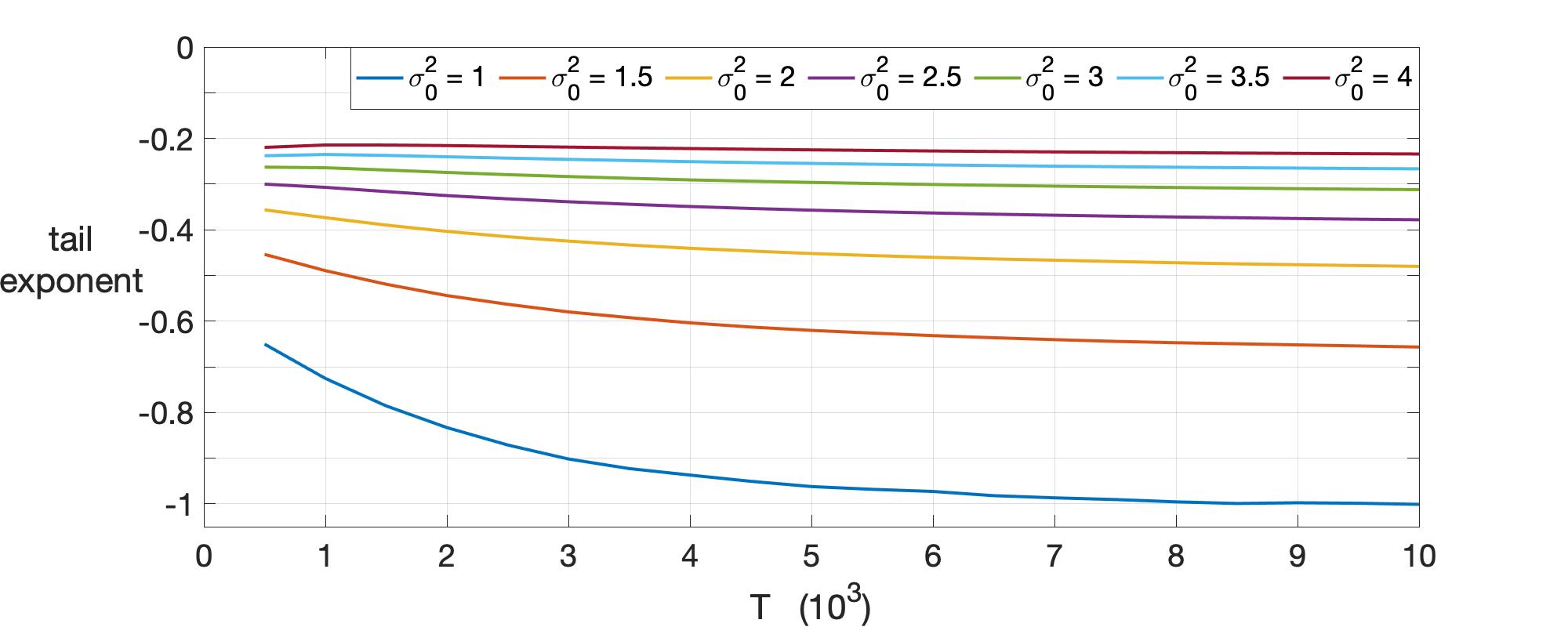
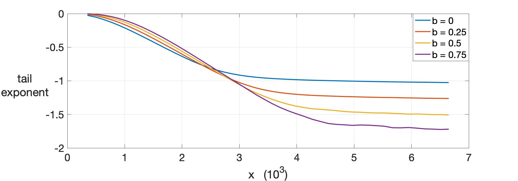
In Corollary 4.2 below, we show that for Gaussian KL-UCB operating in environments with iid Gaussian rewards, if the actual variance is just slightly greater than the variance specified in the algorithm design, then the expected regret will grow at a rate that is a power of $T$. The proof details simplify significantly in this Gaussian setting, and for future reference, we provide a stand-alone proof of Corollary 4.2 in Appendix 12. See Figure 1 in Section 7 for numerical simulations illustrating (32).

Corollary 4.2

Let $\pi$ be KL-UCB optimized for iid Gaussian rewards with variance $\sigma^{2}>0$. Then for any two-armed environment $\nu$ yielding iid Gaussian rewards with actual variance $\sigma_{0}^{2}>0$,

$$\lim_{T\to\infty}\frac{\log\mathbb{P}_{\nu\pi}(N_{r(2)}(T)>x)}{\log(x)}=-\frac{\sigma^{2}}{\sigma_{0}^{2}}$$ (32)

uniformly for $x\in[\log^{1+\gamma}(T),(1-\gamma)T]$ for any $\gamma\in(0,1)$ as $T\to\infty$. So if $\sigma_{0}^{2}>\sigma^{2}$, then for any $a\in(\sigma^{2}/\sigma_{0}^{2},1]$,

$$\liminf_{T\to\infty}\frac{\mathbb{E}_{\nu\pi}[N_{r(2)}(T)]}{T^{1-a}}\geq 1.$$

Corollary 4.2 also holds with $\pi$ as TS designed for iid Gaussian rewards with variance $\sigma^{2}>0$ (and with Gaussian priors on the arm means). In particular, we can obtain this result by using the SLLN’s developed in Fan and Glynn (2022).

4.2 Tail Probability Lower Bounds for General Reward Processes

In this section, we develop supporting results, which are needed in Section 4.3 to establish regret tail characterizations in settings where the dependence structures of rewards are mis-specified. These supporting results can also be used to derive the results in Section 4.1 in settings where the marginal reward distributions are mis-specified. Proposition 4.4 is a SLLN for the regret of KL-UCB operating in an environment with general (possibly non-iid) reward processes that satisfy Assumptions 4.2-4.2 below. KL-UCB is an example of an algorithm that is so-called $\mathcal{M}_{P}$-pathwise convergent, a notion that we introduce in Definition 4.3 below. In Theorem 4.5, we apply our change-of-measure argument to establish lower bounds for the regret tail of such algorithms when operating in an environment with reward processes satisfying Assumptions 4.2-4.2.

We first state a few definitions and assumptions for the reward processes $X_{i}(t)$, $i\in[K]$, $t\geq 1$ that we will work with. For each arm $i$ and sample size $n\geq 1$, define the re-scaled CGF of the sample mean of arm rewards:

$$\mkern 1.5mu\overline{\mkern-1.5mu\Lambda\mkern-1.5mu}\mkern 1.5mu_{i}^{n}(\theta)=\frac{1}{n}\log\;\mathbb{E}\left[\exp\left(\theta\cdot\sum_{t=1}^{n}X_{i}(t)\right)\right].$$

We will assume the following for each arm $i$. The limit $\mkern 1.5mu\overline{\mkern-1.5mu\Lambda\mkern-1.5mu}\mkern 1.5mu_{i}(\theta)=\lim_{n\to\infty}\mkern 1.5mu\overline{\mkern-1.5mu\Lambda\mkern-1.5mu}\mkern 1.5mu_{i}^{n}(\theta)$ exists (possibly infinite) for each $\theta\in\mathbb{R}$, and $0\in\mkern 1.5mu\overline{\mkern-1.5mu\Theta\mkern-1.5mu}\mkern 1.5mu_{i}:=\textnormal{interior}\{\theta\in\mathbb{R}:\mkern 1.5mu\overline{\mkern-1.5mu\Lambda\mkern-1.5mu}\mkern 1.5mu_{i}(\theta)<\infty\}$. $\mkern 1.5mu\overline{\mkern-1.5mu\Lambda\mkern-1.5mu}\mkern 1.5mu_{i}(\cdot)$ is differentiable throughout $\mkern 1.5mu\overline{\mkern-1.5mu\Theta\mkern-1.5mu}\mkern 1.5mu_{i}$, and either $\mkern 1.5mu\overline{\mkern-1.5mu\Theta\mkern-1.5mu}\mkern 1.5mu_{i}=\mathbb{R}$ or $\lim_{m\to\infty}\left|\mkern 1.5mu\overline{\mkern-1.5mu\Lambda\mkern-1.5mu}\mkern 1.5mu_{i}^{\prime}(\theta^{m})\right|=\infty$ for any sequence $\theta^{m}\in\mkern 1.5mu\overline{\mkern-1.5mu\Theta\mkern-1.5mu}\mkern 1.5mu_{i}$ converging to a boundary point of $\mkern 1.5mu\overline{\mkern-1.5mu\Theta\mkern-1.5mu}\mkern 1.5mu_{i}$. These are the conditions ensuring that the Gärtner-Ellis Theorem holds for the sample means of arm rewards (see, for example, Theorem 2.3.6 of Dembo and Zeitouni (1998)). In the context of Assumption 4.2, we refer to the limit $\mkern 1.5mu\overline{\mkern-1.5mu\Lambda\mkern-1.5mu}\mkern 1.5mu_{i}$ as the limiting CGF for arm $i$. In the context of Assumption 4.2, $\mkern 1.5mu\overline{\mkern-1.5mu\Lambda\mkern-1.5mu}\mkern 1.5mu_{i}^{\prime}(0)$, the derivative of limiting CGF evaluated at zero, is the long-run mean reward for arm $i$. Indeed, by the Gärtner-Ellis Theorem and the Borel-Cantelli Lemma,

$$\frac{1}{n}\sum_{t=1}^{n}X_{i}(t)\to\mkern 1.5mu\overline{\mkern-1.5mu\Lambda\mkern-1.5mu}\mkern 1.5mu_{i}^{\prime}(0)$$ (33)

almost surely as $n\to\infty$ for each arm $i$. The optimal arm $r(1)$ is such that $\mkern 1.5mu\overline{\mkern-1.5mu\Lambda\mkern-1.5mu}\mkern 1.5mu_{r(1)}^{\prime}(0)=\max_{i\in[K]}\mkern 1.5mu\overline{\mkern-1.5mu\Lambda\mkern-1.5mu}\mkern 1.5mu_{i}^{\prime}(0)$.

In the current section and in Section 4.3, we also assume for simplicity that the reward process for each arm only evolves forward in time when the arm is played. This ensures that the serial dependence structures of the reward processes are not interrupted in a complicated way by an algorithm’s adaptive sampling schedule, and allows us to determine the limit in Assumption 4.2 for various processes of interest such as Markov chains. Regardless of the specifics of the serial dependence structure of rewards for each arm, we will always assume that there is no dependence between rewards of different arms.

Before stating Proposition 4.4 and Theorem 4.5, we introduce the following notion, which can be compared to the notion of an $\mathcal{M}_{P}$-optimized algorithm in Definition 2.1.

Definition 4.3 (Pathwise Convergent Algorithm)

An algorithm $\pi$ is $\mathcal{M}_{P}$-pathwise convergent if for any environment $\nu$ yielding arm reward sequences $X_{i}(t)$, $i\in[K]$, $t\geq 1$,

$$\left\{\omega:\lim_{n\to\infty}\frac{1}{n}\sum_{t=1}^{n}X_{i}(t)=c_{i},\;i\in[K]\right\}\subset\left\{\omega:\lim_{T\to\infty}\frac{N_{i}(T)}{\log(T)}=\frac{1}{d_{P}(c_{i},\max_{j}c_{j})},\;\forall\;i\neq\mathop{\mathrm{missing}}{argmax}_{j}c_{j}\right\}.$$ (34)

We conjecture that, in general, $\mathcal{M}_{P}$-optimized algorithms are also $\mathcal{M}_{P}$-pathwise convergent. This is directly supported by Proposition 4.4 below, as well as by the SLLN developed for Gaussian TS in Fan and Glynn (2022). It is also suggested by the analysis for developing SLLN’s for non-optimized forced sampling-based algorithms and other UCB algorithms in Cowan and Katehakis (2019). The proof of Proposition 4.4 is based on the arguments in Cowan and Katehakis (2019), and can be found in Appendix 13.

Proposition 4.4

$\mathcal{M}_{P}$-optimized KL-UCB is $\mathcal{M}_{P}$-pathwise convergent.

We now introduce Theorem 4.5, whose proof can be found in Appendix 13. For arm $i$, we use $\mkern 1.5mu\overline{\mkern-1.5mu\Lambda\mkern-1.5mu}\mkern 1.5mu_{i}^{*}$ to denote the convex conjugate of the limiting CGF $\mkern 1.5mu\overline{\mkern-1.5mu\Lambda\mkern-1.5mu}\mkern 1.5mu_{i}$, and we define $\overline{\mathcal{I}}_{i}=\textnormal{interior}\{z\in\mathbb{R}:\mkern 1.5mu\overline{\mkern-1.5mu\Lambda\mkern-1.5mu}\mkern 1.5mu_{i}^{*}(z)<\infty\}$. As mentioned previously, to avoid pathological/trivial situations, we will always assume for each arm $i$ that $\overline{\mathcal{I}}_{i}\subset\mathcal{I}_{P}$ for the chosen base distribution $P$. (We also recall that the convex conjugate of the limiting CGF is the rate function in the Gärtner-Ellis Theorem.)

Theorem 4.5

Let $\pi$ be $\mathcal{M}_{P}$-pathwise convergent. Let the $K$-armed environment $\nu$ yield rewards for each arm that evolve according to any process satisfying Assumptions 4.2-4.2. Then for the $i$-th-best arm $r(i)$,

$$\liminf_{T\to\infty}\inf_{x\in B_{\gamma}(T)}\frac{\log\mathbb{P}_{\nu\pi}(N_{r(i)}(T)>x)}{\log(x)}\geq-\sum_{j=1}^{i-1}\inf_{z\in\overline{\mathcal{I}}_{r(j)}\,:\,z<\mkern 1.5mu\overline{\mkern-1.5mu\Lambda\mkern-1.5mu}\mkern 1.5mu_{r(i)}^{\prime}(0)}\frac{\mkern 1.5mu\overline{\mkern-1.5mu\Lambda\mkern-1.5mu}\mkern 1.5mu^{*}_{r(j)}(z)}{d_{P}(z,\mkern 1.5mu\overline{\mkern-1.5mu\Lambda\mkern-1.5mu}\mkern 1.5mu_{r(i)}^{\prime}(0))},$$ (35)

with $B_{\gamma}(T)=[\log^{1+\gamma}(T),(1-\gamma)T]$ and any $\gamma\in(0,1)$.

Remark 4.6

Whenever we can establish a WLLN for the $N_{i}(T)$ (e.g., as in Proposition 3.11), then our change-of-measure approach can be used to obtain lower bounds on the tail probabilities of the $N_{i}(T)$ (as in Theorems 3.2 and 4.5). The almost sure convergence of the $N_{i}(T)$, as provided by Assumptions 4.2-4.2 (leading to (33)) together with pathwise convergence (in Definition 4.3), is sufficient but not necessary.

4.3 Mis-specified Reward Dependence Structure

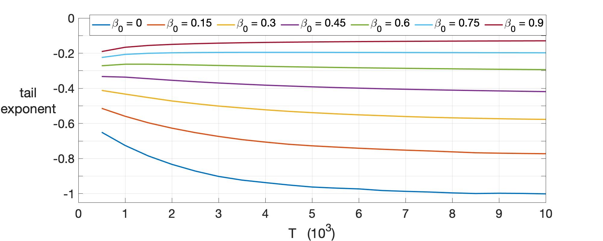
Even if the marginal distributions of the arm rewards are correctly specified, optimized algorithms such as KL-UCB (designed for iid rewards) can still be susceptible to mis-specification of the serial dependence structure. In Corollary 4.7, we provide a lower bound characterization of the regret tail for Gaussian KL-UCB applied to bandits with rewards evolving as Gaussian AR(1) processes. Specifically, for each arm $i$, we assume the rewards evolve as an AR(1) process:

$$X_{i}(t)=\alpha_{i}+\beta_{i}X_{i}(t-1)+W_{i}(t),$$ (36)

where the $\beta_{i}\in(0,1)$ and the $W_{i}(t)$ are iid $N(0,\sigma_{i}^{2})$. The equilibrium distribution for arm $i$ is then $N(\alpha_{i}/(1-\beta_{i}),\sigma_{i}^{2}/(1-\beta_{i}^{2}))$. For simplicity, we assume that the AR(1) reward process for each arm is initialized in equilibrium. So the marginal mean (also the long-run mean as in (33)) for arm $i$ is $\mkern 1.5mu\overline{\mkern-1.5mu\Lambda\mkern-1.5mu}\mkern 1.5mu_{i}^{\prime}(0)=\alpha_{i}/(1-\beta_{i})$. The proof of Corollary 4.7 follows from a straightforward verification of Assumptions 4.2-4.2, which is omitted, and then a direct application of Theorem 4.5.

Corollary 4.7

Let $\pi$ be KL-UCB optimized for iid Gaussian rewards with variance $\sigma^{2}>0$. Then for any two-armed environment $\nu$ yielding rewards that evolve as AR(1) processes (as in (36)),

$$\liminf_{T\to\infty}\inf_{x\in B_{\gamma}(T)}\frac{\log\mathbb{P}_{\nu\pi}(N_{r(2)}(T)>x)}{\log(x)}\geq-\frac{\sigma^{2}}{\sigma_{r(1)}^{2}}(1-\beta_{r(1)})^{2},$$

with $B_{\gamma}(T)=[\log^{1+\gamma}(T),(1-\gamma)T]$ and any $\gamma\in(0,1)$.

To see the effect of mis-specifying the dependence structure, suppose $\sigma_{1}^{2}=\sigma_{2}^{2}=\sigma_{0}^{2}$ and $\beta_{1}=\beta_{2}=\beta_{0}$, for some $\sigma_{0}^{2}>0$ and $\beta_{0}\in(0,1)$, so that the equilibrium distributions for the rewards of both arms are Gaussian with variance $\sigma_{0}^{2}/(1-\beta_{0}^{2})$. Then, even if we specify the same variance $\sigma^{2}=\sigma_{0}^{2}/(1-\beta_{0}^{2})$ in Gaussian KL-UCB, so that the marginal distribution of rewards is correctly specified, we still end up with a tail exponent that is strictly greater than $-1$. This is due to the mis-specification of the serial dependence structure. Specifically, using Corollary 4.7,

$$\liminf_{T\to\infty}\frac{\log\mathbb{P}_{\nu\pi}(N_{r(2)}(T)>T/2)}{\log(T)}\geq-\frac{1-\beta_{0}}{1+\beta_{0}},$$ (37)

and so for any $a\in((1-\beta_{0})/(1+\beta_{0}),1]$,

$$\liminf_{T\to\infty}\frac{\mathbb{E}_{\nu\pi}[N_{r(2)}(T)]}{T^{1-a}}\geq 1.$$

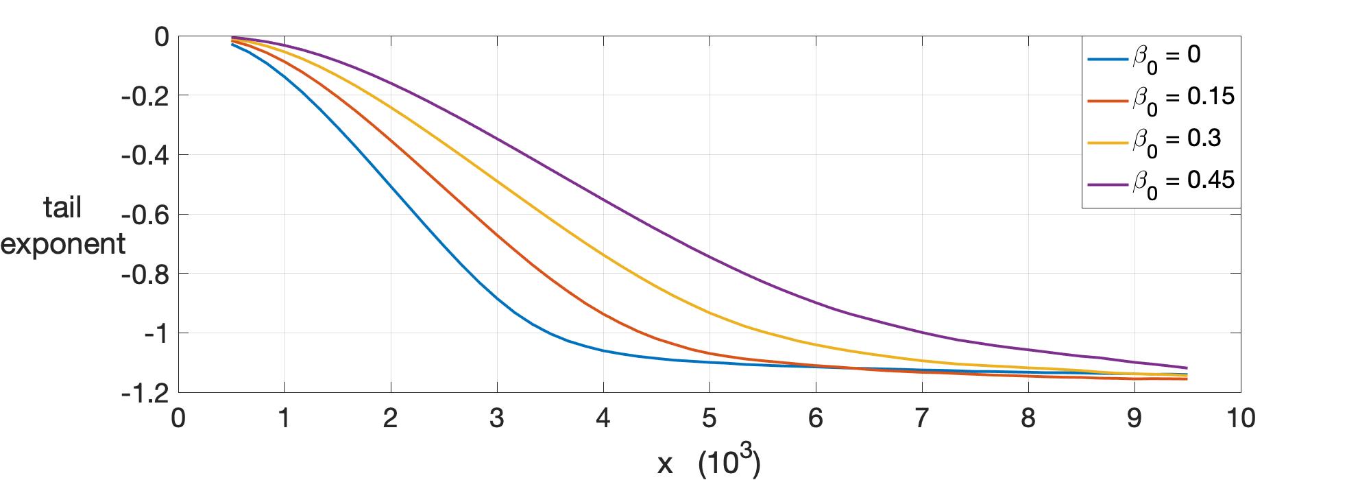
We verify (37) through numerical simulations in Figure 2 in Section 7. The simulations suggest that the lower bound in (37) is tight.

In Corollary 4.8 below, we develop a characterization of the regret tail of KL-UCB operating in an environment $\nu$ with rewards evolving as finite state Markov chains. For each arm $i$, we assume that the rewards evolve as an irreducible Markov chain on a common, finite state space $S\subset\mathbb{R}$, with transition matrix $H_{i}$. For any $\theta\in\mathbb{R}$ and transition matrix $H$, we use $\phi_{H}(\theta)$ to denote the logarithm of the Perron-Frobenius eigenvalue of the corresponding tilted transition matrix:

$$\bigl{(}\exp(\theta\cdot y)H(x,y),\;x,y\in S\bigr{)}.$$ (38)

So in the context of Assumptions 4.2-4.2, $\mkern 1.5mu\overline{\mkern-1.5mu\Lambda\mkern-1.5mu}\mkern 1.5mu_{i}(\theta)=\phi_{H_{i}}(\theta)$ for each arm $i$. (Note that the convex conjugate $\mkern 1.5mu\overline{\mkern-1.5mu\Lambda\mkern-1.5mu}\mkern 1.5mu_{i}^{*}$ of $\mkern 1.5mu\overline{\mkern-1.5mu\Lambda\mkern-1.5mu}\mkern 1.5mu_{i}$ plays the same role in Corollary 4.8 as it does in Theorem 4.5.) For simplicity, we assume that the Markov chain reward process for each arm is initialized in equilibrium. So the marginal mean (also the long-run mean as in (33)) for arm $i$ is $\mkern 1.5mu\overline{\mkern-1.5mu\Lambda\mkern-1.5mu}\mkern 1.5mu_{i}^{\prime}(0)=\phi_{H_{i}}^{\prime}(0)$. Lastly, we wish to ensure that any equilibrium mean between $s_{\text{min}}:=\min S$ and $s_{\text{max}}:=\max S$ can be realized through tilting the transition matrices as in (38). This provides technical convenience, and allows us to use Chernoff-type bounds for Markov chains from the existing literature to derive upper bounds on the regret tail. So we introduce the following notion. We say that a transition matrix $H$ on $S$ satisfies the Doeblin Condition if we have $H(x,s_{\text{min}})>0$ for each $x\neq s_{\text{min}}$, and $H(x,s_{\text{max}})>0$ for each $x\neq s_{\text{max}}$.

The lower bound part of Corollary 4.8 follows from a straightforward verification of Assumptions 4.2-4.2, which is omitted, and then a direct application of Theorem 4.5. To establish the upper bound part, we can again use the proof of Theorem 3.14 (in Section 6.2) and substitute in, where appropriate (in (63) and (68)), a Chernoff-type bound for additive functionals of finite-state Markov chains. One version of such a result that is convenient for our purposes is established in Theorem 1 of Moulos and Anantharam (2019). (Earlier and more general results can be found in Miller (1961) and Kontoyiannis and Meyn (2003), respectively.)

Corollary 4.8

Let $\pi$ be $\mathcal{M}_{P}$-optimized KL-UCB. Let the $K$-armed environment $\nu$ yield rewards for each arm that evolve according to an irreducible Markov chain with a finite state space (with $\mkern 1.5mu\overline{\mkern-1.5mu\Lambda\mkern-1.5mu}\mkern 1.5mu_{i}$ as defined above for each arm $i$), and suppose that the transition matrix for each arm satisfies the Doeblin Condition. Then for the $i$-th-best arm $r(i)$,

$$\lim_{T\to\infty}\frac{\log\mathbb{P}_{\nu\pi}(N_{r(i)}(T)>x)}{\log(x)}=-\sum_{j=1}^{i-1}\inf_{z\in\overline{\mathcal{I}}_{r(j)}\,:\,z<\mkern 1.5mu\overline{\mkern-1.5mu\Lambda\mkern-1.5mu}\mkern 1.5mu_{r(i)}^{\prime}(0)}\frac{\mkern 1.5mu\overline{\mkern-1.5mu\Lambda\mkern-1.5mu}\mkern 1.5mu_{r(j)}^{*}(z)}{d_{P}(z,\mkern 1.5mu\overline{\mkern-1.5mu\Lambda\mkern-1.5mu}\mkern 1.5mu_{r(i)}^{\prime}(0))}$$ (39)

uniformly for $x\in[\log^{1+\gamma}(T),(1-\gamma)T]$ for any $\gamma\in(0,1)$ as $T\to\infty$.

Example 4.9

For the state space $S=\{0,1\}$ (binary rewards), we can examine some numerical values for the right side of (39). Here, we take $d_{P}(z,z^{\prime})$ to be the KL divergence between Bernoulli distributions with means $z$ and $z^{\prime}$. We assume the arm rewards evolve as Markov chains on $S$. So the marginal distributions of the arm rewards are well-specified. Suppose the best arm $r(1)$ evolves according to a transition matrix of the form:

$$H_{r(1)}=\begin{bmatrix}1-q\;\;\;\;\;&q\\ 1-w(q)\;\;\;\;\;&w(q)\end{bmatrix}.$$ (40)

For any $q\leq 0.8$, we set $w(q)\geq 0.8$ such that the chain evolving on $S$ according to $H_{r(1)}$ has equilibrium mean equal to $0.8$. Suppose also that the gap between the equilibrium means of the top two arms, $r(1)$ and $r(2)$, is $\Delta>0$. In Table 1 below, we provide numerical values for the right side of (39) for the case $i=2$ and for different values of $q$ and $\Delta$. As $q$ becomes smaller relative to $0.8$, the autocorrelation in the rewards for arm $r(1)$ becomes more positive, and the resulting regret distribution tail becomes heavier. As the gap $\Delta$ shrinks, the resulting regret tail also becomes heavier. We can see from Table 1 that it is fairly easy (for reasonable values of $q$ and $\Delta$) to obtain regret tails that are heavier than truncated Cauchy (the right side of (39) is greater than $-1$).

		$\Delta$
$q$	$w(q)\quad$	0.12	0.11	0.10	0.09	0.08	0.07	0.06	0.05	0.04
$0.8$	$0.8\quad$	-1.41	-1.37	-1.34	-1.30	-1.26	-1.23	-1.19	-1.16	-1.13
$0.7$	$0.825\quad$	-1.06	-1.03	-1.00	-0.97	-0.95	-0.92	-0.89	-0.87	-0.84
$0.6$	$0.85\quad$	-0.80	-0.78	-0.76	-0.74	-0.72	-0.70	-0.68	-0.66	-0.64
$0.5$	$0.875\quad$	-0.61	-0.59	-0.58	-0.56	-0.54	-0.53	-0.51	-0.50	-0.49

Table 1: For arm rewards evolving as Markov chains on the state space $S=\{0,1\}$, and with $d_{P}$ being the Bernoulli KL divergence, we provide numerical values for the right side of (39). Here, $i=2$, and we consider different values of $q$ (as used in the best arm’s transition matrix $H_{r(1)}$ in (40)) and $\Delta$ (the gap between the equilibrium means of the two best arms, $r(1)$ and $r(2)$).

4.4 Higher Moments

In this section, we point out that the $1+\delta$ moment of regret for any $\delta>0$ must grow roughly as $T^{\delta}$. Contrary to what one might conjecture in light of the WLLN that we saw in Proposition 3.11, the $1+\delta$ moment of regret is not poly-logarithmic. In Corollary 4.10 below, which is a direct consequence of Theorem 3.2, we show that expected regret minimization does not provide any help in controlling higher moments of regret. It forces the tail of the regret distribution to be as heavy as possible while ensuring the expected regret scales as $\log(T)$ (as we saw in Theorem 3.2 and Corollary 3.10). Consequently, there is no control over the distribution tails of $1+\delta$ powers of regret, and thus no uniform integrability of $1+\delta$ powers of regret (normalized by $\log^{1+\delta}(T)$).

Corollary 4.10

Let $\pi$ be $\mathcal{M}_{P}$-optimized. Suppose also that $P$ is discrimination equivalent. Then for any environment $\nu\in\mathcal{M}_{P}^{K}$, and any $\delta>0$ and $\delta^{\prime}\in(0,\delta)$,

$$\liminf_{T\to\infty}\frac{\mathbb{E}_{\nu\pi}[N_{r(2)}(T)^{1+\delta}]}{T^{\delta^{\prime}}}\geq 1.$$

5 Improvement of the Regret Distribution Tail

In Sections 3 and 4, we have seen how optimized algorithms prioritize expected regret minimization at the cost of rendering the tail of the regret distribution susceptible to even small degrees of model mis-specification. In Section 5, we discuss a general approach to make the regret tail lighter (with a more negative tail exponent), which as we show, leads to a degree of robustness to model mis-specification. Specifically, in Section 5.1, we describe a simple way to construct a UCB algorithm so that the regret tail exponent is $-(1+b)$ (or less) for any desired $b>0$, for an exponential family class of environments. We then show how this also makes the regret tail suitably lighter uniformly over a general class of environments. In Section 5.2, we show that the modification provides protection against mis-specification of the arm reward distributions in iid settings. In Section 5.3, we show that such modification also provides protection against Markovian departures from independence of the arm rewards. Our analysis further establishes an explicit trade-off between the amount of UCB exploration (and expected regret) and the resulting heaviness of the regret tail (see Remarks 5.5 and 5.6).

5.1 A Simple Approach to Obtain Lighter Regret Tails

In this section, and in Sections 5.2 and 5.3, we focus on Algorithm 1, which is a simple modification of the KL-UCB algorithm (Algorithm 2 of Cappé et al. (2013)). Like KL-UCB, Algorithm 1 is defined for any exponential family $\mathcal{M}_{P}$, as in (1)-(2). However, the difference is that Algorithm 1 involves re-scaling the KL divergence $d_{P}$ by $1/(1+b)$, for a desired $b>0$. This has the effect of inducing additional exploration, and is equivalent to increasing the “radius” of the upper confidence bound by a factor of $1+b$; see also Remark 5.5 towards the end of this section.

Algorithm 1 : $b$-robustified KL-UCB (based on Algorithm 2 of Cappé et al. (2013))

input: $b\geq 0$, $d_{P}:\mathcal{I}_{P}\times\mathcal{I}_{P}\to[0,\infty)$

initialize: Play each arm $1,\dots,K$ once

for $t\geq K$ do

     Play the arm (with ties broken arbitrarily):

$$A(t+1)=\mathop{\mathrm{missing}}{argmax}_{i\in[K]}\;\sup\left\{z\in\mathcal{I}_{P}:\frac{d_{P}(\widehat{\mu}_{i}(t),z)}{1+b}\leq\frac{\log(1+t\log^{2}(t))}{N_{i}(t)}\right\}$$

end for

Using Algorithm 1, we can ensure that the regret tail exponent is $-(1+b)$ (or less) for all environments in $\mathcal{M}_{P}^{K}$. This follows from a direct adaptation of Proposition 4.1. Specifically, with $\pi$ as Algorithm 1, we have for any environment $\nu=(P^{\mu_{1}},\dots,P^{\mu_{K}})\in\mathcal{M}_{P}^{K}$ and the $i$-th-best arm $r(i)$,

$$\lim_{T\to\infty}\frac{\log\mathbb{P}_{\nu\pi}(N_{r(i)}(T)>x)}{\log(x)} =-(1+b)\sum_{j=1}^{i-1}\inf_{z\in\mathcal{I}_{P}\,:\,z<\mu_{r(i)}}\frac{d_{P}(z,\mu_{r(j)})}{d_{P}(z,\mu_{r(i)})}$$ (41)

$$\leq-(1+b)(i-1)$$

uniformly for $x\in[\log^{1+\gamma}(T),(1-\gamma)T]$ for any $\gamma\in(0,1)$ as $T\to\infty$. The numerators in the infima of (41) can be compared to those of (31) in Proposition 4.1. In Figure 4 in Section 7, we provide numerical simulations that illustrate the result (41) when $\mathcal{M}_{P}$ is a Gaussian family.

Furthermore, using Algorithm 1, we can ensure that the regret tail exponent is $-(1+b)$ (or less) for all environments in a class $\mathcal{M}_{P,0}^{K}$ that is larger than $\mathcal{M}_{P}^{K}$. This is established in Corollary 5.3 below. Here, $\mathcal{M}_{P,0}$ is a general family of distributions, whose CGF’s are dominated by those of $\mathcal{M}_{P}$:

$$\mathcal{M}_{P,0}=\left\{Q:\mu(Q)\in\mathcal{I}_{P},\;\Lambda_{Q}(\theta)\leq\Lambda_{P^{\mu(Q)}}(\theta)\;\;\forall\;\theta\in\mathbb{R}\right\}.$$ (42)

(Recall that $\Lambda_{P^{\mu(Q)}}$ is the CGF of $P^{\mu(Q)}$, the distribution resulting from tilting $P$ to have mean $\mu(Q)$, as in (1).) We have the following examples of $\mathcal{M}_{P}$ and $\mathcal{M}_{P,0}$.

Example 5.1

Let $\mathcal{M}_{P}$ be the Gaussian family with variance $\sigma^{2}$. Then $\mathcal{M}_{P,0}$ is the family of all sub-Gaussian distributions with variance proxy $\sigma^{2}$. (We say $Z$ is sub-Gaussian with variance proxy $\sigma^{2}$ if $\mathbb{E}[e^{\theta(Z-\mathbb{E}[Z])}]\leq e^{\sigma^{2}\theta^{2}/2}$ for all $\theta\in\mathbb{R}$.)

Example 5.2

Let $\mathcal{M}_{P}$ be the Bernoulli family. Then $\mathcal{M}_{P,0}$ is the family of all distributions supported on a subset of $[0,1]$.

Corollary 5.3 follows from a direct adaptation of the proof of Proposition 4.1, similar to the justification for (41). This is because the distributions in $\mathcal{M}_{P,0}$ obey the same Chernoff bounds as those in $\mathcal{M}_{P}$, per the definition in (42).

Corollary 5.3

Let $\pi$ be Algorithm 1, with divergence $d_{P}$ and $b\geq 0$. Then for any environment $\nu=(Q_{1},\dots,Q_{K})\in\mathcal{M}_{P,0}^{K}$ and the $i$-th-best arm $r(i)$,

$$\lim_{T\to\infty}\frac{\log\mathbb{P}_{\nu\pi}(N_{r(i)}(T)>x)}{\log(x)} =-(1+b)\sum_{j=1}^{i-1}\inf_{z\in\mathcal{I}_{Q_{r(j)}}\,:\,z<\mu(Q_{r(i)})}\frac{d_{Q_{r(j)}}(z,\mu(Q_{r(j)}))}{d_{P}(z,\mu(Q_{r(i)}))}$$ (43)

$$\leq-(1+b)(i-1)$$

uniformly for $x\in[\log^{1+\gamma}(T),(1-\gamma)T]$ for any $\gamma\in(0,1)$ as $T\to\infty$.

Remark 5.4

The $-(1+b)(i-1)$ upper bound on (43) is due to the fact that the ratios in the infima of (43) are at least $1$. This is because for any $Q\in\mathcal{M}_{P,0}$,

$$d_{Q}(z,\mu(Q)) =\sup_{\theta\in\mathbb{R}}\{\theta z-\Lambda_{Q}(\theta)\}$$

$$\geq\sup_{\theta\in\mathbb{R}}\{\theta z-\Lambda_{P^{\mu(Q)}}(\theta)\}=d_{P}(z,\mu(Q)),$$

where the inequality follows from the definition of $\mathcal{M}_{P,0}$ in (42).

Remark 5.5

From (41) and (43), we see there is an explicit trade-off between the amount of exploration and the resulting heaviness of the regret distribution tail. Specifically, using the re-scaled divergence function $d_{P}/(1+b)$ instead of $d_{P}$ in Algorithm 1 is equivalent to increasing the amount of UCB exploration by $1+b$ times, which for a fixed instance of bandit environment $\nu$, yields a regret tail exponent of $-C(\nu)\cdot(1+b)$, where $C(\nu)\geq 1$ is a constant depending on $\nu$. While studying a related problem, Audibert et al. (2009) developed finite-time upper bounds on the tail of the regret distribution for the UCB1 algorithm (due to Auer et al. (2002)) in the bounded rewards setting, which are suggestive of the exploration-regret tail trade-off that we provide in (41) and (43). However, they do not develop matching lower bounds for the regret tail. Such lower bounds are a fundamental ingredient in establishing the nature of the trade-off.

Remark 5.6

As expected from Proposition 3.21, aiming for a lighter regret tail does come at the cost of greater expected regret. However, the expected regret increase is modest, being only a multiple of $\log(T)$. And one benefit is greater robustness to model mis-specification, as we will see in the next two sections. (As a follow-up to Corollary 5.3, we have a precise characterization of the expected regret growth of Algorithm 1 in (48) of Corollary 5.9 in the next section.)

5.2 Robustness to Mis-specified Reward Distribution

For an $\mathcal{M}_{P}$-optimized algorithm, if the true reward distributions do not belong in $\mathcal{M}_{P}$, then the regret tails can be heavier than truncated Cauchy, resulting in expected regret that grows as a power of the time horizon $T$. As we saw in Section 4.1 via Proposition 4.1 and Corollary 4.2, one example of this is when the variance in the design of KL-UCB for Gaussian bandits is just slightly under-specified relative to the true variance. To alleviate such issues, we can use Algorithm 1. We will see in Corollary 5.9 below that this provides protection against distributional mis-specification of the arm rewards. In particular, we can maintain logarithmic expected regret for environments from an enlarged class $\mathcal{M}_{P,b}^{K}$, which is defined in (44) below and depends on the chosen value of $b>0$ in Algorithm 1.

The enlarged family of distributions is:

$$\mathcal{M}_{P,b}=\left\{Q\,:\,\mu(Q)\in\mathcal{I}_{P},\;\Lambda_{Q}(\theta)\leq\Psi_{P,b}(\mu(Q),\theta)\;\;\forall\;\theta\in\mathbb{R}\right\},$$ (44)

where for any distribution $Q$ and $z\in\mathcal{I}_{Q}$, we define:

$$\Psi_{Q,b}(z,\theta)=\frac{\Lambda_{Q^{z}}((1+b)\theta)}{1+b},\quad\theta\in\mathbb{R}.$$ (45)

Setting $b=0$ recovers $\mathcal{M}_{P,0}$ as in (42). Using Jensen’s inequality and the definition in (45), it is straightforward to see that $\mathcal{M}_{P}\subsetneqq\mathcal{M}_{P,b}$ for $b>0$. Moreover, with $\mathcal{M}_{P,0}$ from (42) and any $b^{\prime}>b>0$, we have $\mathcal{M}_{P,0}\subsetneqq\mathcal{M}_{P,b}\subsetneqq\mathcal{M}_{P,b^{\prime}}$. An example of $\mathcal{M}_{P}$ and $\mathcal{M}_{P,b}$ is the following.

Example 5.7

Let $\mathcal{M}_{P}$ be the Gaussian family with variance $\sigma^{2}$. Then $\mathcal{M}_{P,b}$ is the family of all sub-Gaussian distributions with variance proxy $\sigma^{2}(1+b)$. (Also, $\mathcal{M}_{P,0}$ is the family of all sub-Gaussian distributions with variance proxy $\sigma^{2}$, as we saw in Example 5.1.)

Remark 5.8

Algorithm 1 uses the divergence $d_{P}$ re-scaled by $1/(1+b)$. This is directly related to the re-scaled CGF’s in (45), namely $y\mapsto d_{P}(y,z)/(1+b)$ is the convex conjugate of $\theta\mapsto\Psi_{P,b}(z,\theta)$, as seen via:

$$\frac{d_{P}(y,z)}{1+b} =\frac{1}{1+b}\cdot\sup_{\theta\in\mathbb{R}}\left\{\theta y-\Lambda_{P^{z}}(\theta)\right\}=\sup_{\theta\in\mathbb{R}}\{\theta y-\Psi_{P,b}(z,\theta)\}.$$ (46)

In Corollary 5.9, (47) can be obtained by using a straightforward adaptation of the proof of Theorem 10.6 in book by Lattimore and Szepesvári (2020). The proof there is developed for KL-UCB in the iid Bernoulli rewards setting. However, the proof can be directly extended to cover KL-UCB for any exponential family by using a Chernoff bound based on the KL divergence for that family. Moreover, the proof can be directly adapted to our setting in Corollary 5.9 using $d_{P}/(1+b)$ as the divergence in the Chernoff bound. Due to (44)-(46), the distributions in $\mathcal{M}_{P,b}$ obey a Chernoff bound that involves the re-scaled divergence $d_{P}/(1+b)$. Then, (48) follows from Corollary 5.3 and Proposition 3.21.

Corollary 5.9

Let $\pi$ be Algorithm 1, with divergence $d_{P}$ and $b\geq 0$. Then for any environment $\nu=(Q_{1},\dots,Q_{K})\in\mathcal{M}_{P,b}^{K}$ and each sub-optimal arm $i$,

$$\limsup_{T\to\infty}\frac{\mathbb{E}_{\nu\pi}\left[N_{i}(T)\right]}{\log(T)}\leq\frac{1+b}{d(\mu(Q_{i}),\mu_{*}(\nu))}.$$ (47)

Moreover, for any environment $\nu=(Q_{1},\dots,Q_{K})\in\mathcal{M}_{P,0}^{K}$ and each sub-optimal arm $i$,

$$\lim_{T\to\infty}\frac{\mathbb{E}_{\nu\pi}\left[N_{i}(T)\right]}{\log(T)}=\frac{1+b}{d(\mu(Q_{i}),\mu_{*}(\nu))}.$$ (48)

5.3 Robustness to Mis-specified Reward Dependence Structure

In this section, we consider arm rewards taking values in a finite set $S\subset\mathbb{R}$. Let $P$ be a distribution on $S$. Even if the marginal distributions of arm rewards belong in the exponential family $\mathcal{M}_{P}$, the serial dependence structure of rewards could be mis-specified, which can result in regret tails that are heavier than truncated Cauchy, and expected regret that grows as a power of the time horizon $T$. We saw an example of this in Section 4.3 via Corollary 4.8, particularly via Example 4.9. To alleviate such issues, we use Algorithm 1. We will see in Corollary 5.10 below that this provides protection against Markovian departures from independence of the arm rewards. In particular, we can maintain logarithmic expected regret when the arm rewards evolve as Markov chains with transition matrices from a set $\widetilde{\mathcal{M}}_{P,b}$, which is defined in (49) below and depends on the chosen value of $b\geq 0$ in Algorithm 1.

Let $\mathcal{S}_{\left|S\right|}$ denote the set of $\left|S\right|\times\left|S\right|$ irreducible stochastic matrices satisfying the Doeblin Condition (as discussed in Section 4.3 in the context of Corollary 4.8). We define

$$\widetilde{\mathcal{M}}_{P,b}=\left\{H\in\mathcal{S}_{\left|S\right|}\,:\,\phi_{H}(\theta)\leq\Psi_{P,b}(\phi_{H}^{\prime}(0),\theta)\;\;\forall\;\theta\in\mathbb{R}\right\},$$ (49)

and we recall that $\phi_{H}(\theta)$ is the logarithm of the Perron-Frobenius eigenvalue of the tilted version (as in (38)) of transition matrix $H$, and $\phi_{H}^{\prime}(0)$ is the equilibrium mean of a chain with transition matrix $H$. Of course, the exponential family $\mathcal{M}_{P}$ is equivalent to a strict subset of the collection of transition matrices with identical rows in $\widetilde{\mathcal{M}}_{P,b}$, for any $b>0$. Also, for any $b^{\prime}>b>0$, $\widetilde{\mathcal{M}}_{P,b}\subsetneqq\widetilde{\mathcal{M}}_{P,b^{\prime}}$. In Example 5.11, which is given after Corollary 5.10, we examine the degree to which $\widetilde{\mathcal{M}}_{P,b}$ is “larger” than $\mathcal{M}_{P}$ when $S=\{0,1\}$ and $\mathcal{M}_{P}$ is the Bernoulli family.

We have Corollary 5.10 below, which (like Corollary 5.9) can also be obtained by using a straightforward adaptation of the proof of Theorem 10.6 in Lattimore and Szepesvári (2020) (using $d_{P}/(1+b)$ as the divergence). Theorem 1 of Moulos and Anantharam (2019) provides a Chernoff bound for additive functionals of finite state space Markov chains that is convenient for this purpose. (As mentioned previously, earlier and more general results can be found in Miller (1961) and Kontoyiannis and Meyn (2003), respectively.) Due to (49) and (45)-(46), Markov chains with transition matrices in $\widetilde{\mathcal{M}}_{P,b}$ obey this Chernoff bound, which involves the re-scaled divergence $d_{P}/(1+b)$.

Corollary 5.10

Let $\pi$ be Algorithm 1, with divergence $d_{P}$ and $b\geq 0$. For the $K$-armed environment $\nu$, suppose arm $i$ yields rewards that evolve according to a Markov chain with transition matrix $H_{i}\in\widetilde{\mathcal{M}}_{P,b}$. Then for any sub-optimal arm $i$,

$$\limsup_{T\to\infty}\frac{\mathbb{E}_{\nu\pi}\left[N_{i}(T)\right]}{\log(T)}\leq\frac{1+b}{d_{P}(\phi_{H_{i}}^{\prime}(0),\phi_{H_{r(1)}}^{\prime}(0))}.$$

Example 5.11

Let the state space $S=\{0,1\}$, and let $\mathcal{M}_{P}$ be the Bernoulli family of distributions. Consider transition matrices on $S$ of the form:

$$H=\begin{bmatrix}1-q\;\;\;\;\;&q\\ 1-q^{\prime}\;\;\;\;\;&q^{\prime}\end{bmatrix}.$$ (50)

The more positive the difference $q^{\prime}-q$, the more positive the autocorrelation between the rewards. In Table 2 below, for different values of $b>0$, we examine how positive the difference $q^{\prime}-q$ can be in order for $H$ to still belong in $\widetilde{\mathcal{M}}_{P,b}$, and thus for Corollary 5.10 to be applicable. As the targeted regret tail exponent $-(1+b)$ is made more negative, the algorithm can withstand more positive autocorrelation between the rewards and still maintain logarithmic expected regret.

$-(1+b)\qquad$	-2	-3	-4	-5	-6	-7	-8	-9	-10	-11
$\text{max allowed }q^{\prime}-q\qquad$	0.18	0.36	0.49	0.59	0.65	0.70	0.74	0.77	0.80	0.82

Table 2: For particular $-(1+b)$ values (upper bound on the regret tail exponent), and for the restriction $q,q^{\prime}\in[0.05,0.95]$, we give the maximum allowed difference $q^{\prime}-q$ that ensures the transition matrix $H$ in (50) belongs in $\widetilde{\mathcal{M}}_{P,b}$, as defined in (49) (and (45)).

Remark 5.12

For general reward processes satisfying Assumptions 4.2-4.2, e.g., general Markov processes, there are no finite-sample concentration bounds. So there does not seem to be a universal way to obtain an upper bound on the regret tail to complement the lower bound in Theorem 4.5 (unlike in Proposition 4.1 and Corollary 4.8). For such reward processes, there also does not seem to be a universal way to obtain upper bounds on expected regret such as in Corollary 5.10, and thus there are no provable robustness benefits for our procedure to lighten the regret tail. Nevertheless, our simulations in Figure 5 in Section 7 suggest that we can still ensure the regret tail is lighter to a desired level using our procedure. (The lower bound in Theorem 4.5 seems to be tight in greater generality than what we are able to provably show.)

6 Proofs of Theorems 3.2 and 3.14

6.1 Proof of Theorem 3.2

Without loss of generality, suppose that $\mu_{1}>\mu_{2}>\dots>\mu_{K}$ (i.e., $r(i)=i$ for all $i\in[K]$) in the environment $\nu=(P^{\mu_{1}},P^{\mu_{2}},\dots,P^{\mu_{K}})$. We first show (7) and (8) for second-best arm $i=2$. Consider the alternative environment $\widetilde{\nu}=(P^{\widetilde{\mu}_{1}},P^{\mu_{2}},\dots,P^{\mu_{K}})$, where $\widetilde{\mu}_{1}<\mu_{2}$, and $\mu_{2},\dots,\mu_{K}$ are the same mean values from the original environment $\nu$. (Arm 2 is the best arm in $\widetilde{\nu}$.) Later in the proof, we will consider different values for $\widetilde{\mu}_{1}$, subject to $\widetilde{\mu}_{1}<\mu_{2}$ and $\widetilde{\mu}_{1}\in\mathcal{I}_{P}$. Let $\delta>0$, and define the events:

$$\mathcal{A}_{T}=\left\{\left|\frac{N_{1}(T)}{\log(T)}-\frac{1}{d_{P}(\widetilde{\mu}_{1},\mu_{2})}\right|\leq\delta\right\}\cap\left\{\left|\frac{N_{j}(T)}{\log(T)}-\frac{1}{d_{P}(\mu_{j},\mu_{2})}\right|\leq\delta,\;\forall\;j\geq 3\right\}$$

$$\mathcal{B}_{T}=\left\{\left|\frac{1}{N_{1}(T)}\sum_{t=1}^{N_{1}(T)}\log\frac{dP^{\mu_{1}}}{dP^{\widetilde{\mu}_{1}}}(X_{1}(t))+d_{P}(\widetilde{\mu}_{1},\mu_{1})\right|\leq\delta\right\}.$$

By a change of measure from $\nu$ to $\widetilde{\nu}$,

$$\mathbb{P}_{\nu\pi}(N_{2}(T)>(1-\gamma)T) =\mathbb{E}_{\widetilde{\nu}\pi}\left[\mathbb{I}\left({N_{2}(T)>(1-\gamma)T}\right)\prod_{t=1}^{N_{1}(T)}\frac{dP^{\mu_{1}}}{dP^{\widetilde{\mu}_{1}}}(X_{1}(t))\right]$$ (51)

$$\geq\mathbb{E}_{\widetilde{\nu}\pi}\left[\mathbb{I}\left({\mathcal{A}_{T},\mathcal{B}_{T}}\right)\exp\left(\frac{1}{N_{1}(T)}\sum_{t=1}^{N_{1}(T)}\log\frac{dP^{\mu_{1}}}{dP^{\widetilde{\mu}_{1}}}(X_{1}(t))\cdot N_{1}(T)\right)\right]$$ (52)

$$\geq\mathbb{P}_{\widetilde{\nu}\pi}(\mathcal{A}_{T},\mathcal{B}_{T})\cdot\exp\left(-\left(d_{P}(\widetilde{\mu}_{1},\mu_{1})+\delta\right)\left(\frac{1}{d_{P}(\widetilde{\mu}_{1},\mu_{2})}+\delta\right)\log(T)\right).$$ (53)

where (52) follows from $\{N_{2}(T)>(1-\gamma)T\}\supset\mathcal{A}_{T}$ for sufficiently large $T$, and (53) follows from lower bounds using $\mathcal{A}_{T}$ and $\mathcal{B}_{T}$. From (53), taking logs and dividing by $\log(T)$,

$$\frac{\log\mathbb{P}_{\nu\pi}(N_{2}(T)>(1-\gamma)T)}{\log(T)}\geq\frac{\log\mathbb{P}_{\widetilde{\nu}\pi}(\mathcal{A}_{T},\mathcal{B}_{T})}{\log(T)}-\left(d_{P}(\widetilde{\mu}_{1},\mu_{1})+\delta\right)\left(\frac{1}{d_{P}(\widetilde{\mu}_{1},\mu_{2})}+\delta\right).$$ (54)

Using Proposition 3.11 together with the WLLN for sample means, we have $\lim_{T\to\infty}\mathbb{P}_{\widetilde{\nu}\pi}(\mathcal{A}_{T},\mathcal{B}_{T})=1$. So the first term on the right side of (54) is negligible as $T\to\infty$, and upon sending $\delta\downarrow 0$ and optimizing with respect to $\widetilde{\mu}_{1}$, we have

$$\liminf_{T\to\infty}\frac{\log\mathbb{P}_{\nu\pi}(N_{2}(T)>(1-\gamma)T)}{\log(T)} \geq-\inf_{\widetilde{\mu}_{1}\in\mathcal{I}_{P}\,:\,\widetilde{\mu}_{1}<\mu_{2}}\frac{d_{P}(\widetilde{\mu}_{1},\mu_{1})}{d_{P}(\widetilde{\mu}_{1},\mu_{2})}.$$ (55)

The conclusion (7) holds with the infimum over $B_{\gamma}(T)=[T^{\gamma},(1-\gamma)T]$ due to $x\mapsto\log\mathbb{P}_{\nu\pi}(N_{2}(T)>x)/\log(x)$ being monotone decreasing for $x\in B_{\gamma}(T)$, with $T$ fixed.

We now establish (8). Because $P$ is discrimination equivalent, the right side of (55) is equal to $-1$. Because $\pi$ is $\mathcal{M}_{P}$-optimized, using Markov’s inequality, the case $x=(1-\gamma)T$ in (8) is established, i.e.,

$$\lim_{T\to\infty}\frac{\log\mathbb{P}_{\nu\pi}(N_{2}(T)>(1-\gamma)T)}{\log((1-\gamma)T)}=-1.$$ (56)

To obtain the uniform result for $x\in[T^{\gamma},(1-\gamma)T]$, note that for $T>T^{\gamma}/(1-\gamma)$,

$$\mathbb{P}_{\nu\pi}(N_{2}(T)>T^{\gamma})\geq\mathbb{P}_{\nu\pi}(N_{2}(\lceil T^{\gamma}/(1-\gamma)\rceil)>T^{\gamma}).$$ (57)

Using (56), but with $\lceil T^{\gamma}/(1-\gamma)\rceil$ in the place of $T$, together with Markov’s inequality (with $\pi$ being $\mathcal{M}_{P}$-optimized),

$$\lim_{T\to\infty}\frac{\log\mathbb{P}_{\nu\pi}(N_{2}(\lceil T^{\gamma}/(1-\gamma)\rceil)>T^{\gamma})}{\log(T^{\gamma})}=-1.$$

Thus, using (57) and Markov’s inequality (with $\pi$ being $\mathcal{M}_{P}$-optimized), the case $x=T^{\gamma}$ in (8) is established, i.e.,

$$\lim_{T\to\infty}\frac{\log\mathbb{P}_{\nu\pi}(N_{2}(T)>T^{\gamma})}{\log(T^{\gamma})}=-1.$$ (58)

Since, for each $T$, $x\mapsto\log\mathbb{P}_{\nu\pi}(N_{2}(T)>x)/\log(x)$ is a monotone decreasing function for $x>1$, the desired uniform convergence in (8) for $x\in[T^{\gamma},(1-\gamma)T]$ follows from the matching limits at the endpoints $x=(1-\gamma)T$ and $x=T^{\gamma}$, as established in (56) and (58), respectively.

We now show (7) for sub-optimal arm $i\geq 3$. Consider the alternative environment $\widetilde{\nu}=(P^{\widetilde{\mu}_{1}},\dots,P^{\widetilde{\mu}_{i-1}},P^{\mu_{i}},\dots,P^{\mu_{K}})$, where $\widetilde{\mu}_{j}<\mu_{i}$ for all $j\leq i-1$, and $\mu_{i},\dots,\mu_{K}$ are the same mean values from the original environment $\nu$. (Arm $i$ is now the best arm in $\widetilde{\nu}$.) The events $\mathcal{A}_{T}$ and $\mathcal{B}_{T}$ become:

$$\mathcal{A}_{T} =\left\{\left|\frac{N_{j}(T)}{\log(T)}-\frac{1}{d_{P}(\widetilde{\mu}_{j},\mu_{i})}\right|\leq\delta,\;\forall\;j\leq i-1\right\}\cap\left\{\left|\frac{N_{j}(T)}{\log(T)}-\frac{1}{d_{P}(\mu_{j},\mu_{i})}\right|\leq\delta,\;\forall\;j\geq i+1\right\}$$

$$\mathcal{B}_{T} =\left\{\left|\frac{1}{N_{j}(T)}\sum_{t=1}^{N_{j}(T)}\log\frac{dP^{\mu_{j}}}{dP^{\widetilde{\mu}_{j}}}(X_{j}(t))+d_{P}(\widetilde{\mu}_{j},\mu_{j})\right|\leq\delta,\;\forall\;j\leq i-1\right\}.$$

To obtain (7) for sub-optimal arm $i\geq 3$, we can then run through arguments analogous to those in (51)-(55). Here, the change of measure from $\nu$ to $\widetilde{\nu}$ involves the product of $i-1$ likelihood ratios corresponding to the arms $1,\dots,i-1$. Each of the parameter values $\widetilde{\mu}_{1},\dots,\widetilde{\mu}_{i-1}$ can be optimized separately (subject to $\widetilde{\mu}_{j}<\mu_{i}$ and $\widetilde{\mu}_{j}\in\mathcal{I}_{P}$ for all $j\leq i-1$) to yield the desired conclusion.

6.2 Proof of Theorem 3.14

Without loss of generality, suppose that $\mu_{1}>\mu_{2}>\dots>\mu_{K}$ (i.e., $r(i)=i$ for all $i\in[K]$). Define for arm $i$ the KL-UCB index at time $t$, given that arm $i$ has been played $n$ times:

$$\widetilde{U}_{i}(n,t)=\sup\left\{z\in\mathcal{I}_{P}:d_{P}(\widehat{\mu}_{i}(\tau_{i}(n)),z)\leq\frac{f(t)}{n}\right\},$$

where $\tau_{i}(n)$ denotes the time of the $n$-th play of arm $i$, and as defined previously, $\widehat{\mu}_{i}(t)=\frac{1}{N_{i}(t)}\sum_{s=1}^{N_{i}(t)}X_{i}(s)$. Here, we use the choice $f(t)=\log(t)$, where (as in Algorithm 2 of Cappé et al. (2013)) the “exploration function” $f(t)$ is a design choice. Section 7 of Cappé et al. (2013) recommends using this particular choice of $f(t)$. Moreover, our proof below can easily accommodate other choices such as $f(t)=\log(t)+3\log\log(t)$ (used in Theorem 1 of Cappé et al. (2013)), or $f(t)=\log(1+t\log^{2}(t))$ (used in Theorem 10.6 of Lattimore and Szepesvári (2020)). Using any one of these variations of $f(t)$ does not affect the conclusion of our Theorem 3.14.

We first show (18) for the sub-optimal arm $i=2$. Let $x_{T}=\left\lfloor\log^{1+\gamma}(T)\right\rfloor$ with fixed $\gamma\in(0,1)$. Also, let $\delta\in(0,\mu_{1}-\mu_{2})$. We have the following bounds:

$$\mathbb{P}_{\nu\pi}\left(N_{2}(T)>x_{T}\right) \leq\mathbb{P}_{\nu\pi}\Bigl{(}\exists\;t\in(\tau_{2}(x_{T}),T]\;\;\;\text{s.t.}\;\;\;\widetilde{U}_{1}(N_{1}(t-1),t-1)\leq\widetilde{U}_{2}(N_{2}(t-1),t-1)\Bigr{)}$$ (59)

$$\leq\mathbb{P}_{\nu\pi}\Bigl{(}\exists\;t\in(x_{T},T]\;\;\;\text{s.t.}\;\;\;\widetilde{U}_{1}(N_{1}(t-1),x_{T})\leq\widetilde{U}_{2}(x_{T},T)\Bigr{)}$$

$$\leq\mathbb{P}_{\nu\pi}\Bigl{(}\exists\;t\in(x_{T},T]\;\;\;\text{s.t.}\;\;\;\widetilde{U}_{1}(N_{1}(t-1),x_{T})\leq\mu_{2}+\delta\Bigr{)}$$ (60)

$$\quad+\mathbb{P}_{\nu\pi}\Bigl{(}\widetilde{U}_{2}(x_{T},T)>\mu_{2}+\delta\Bigr{)}.$$ (61)

Note that (59) holds because $N_{2}(T)>x_{T}$ is the event of interest, and so after the $x_{T}$-th play of arm $2$ at time $\tau_{2}(x_{T})$, there must be at least one more time period in which arm $2$ is played.

For the term in (60), we have

$$(\ref{term6}) \leq\sum_{m=1}^{\infty}\mathbb{P}_{\nu\pi}\Bigl{(}\widetilde{U}_{1}(m,x_{T})\leq\mu_{2}+\delta\Bigr{)}$$ (62)

$$=\sum_{m=1}^{\infty}\mathbb{P}_{\nu\pi}\left(d_{P}(\widehat{\mu}_{1}(\tau_{1}(m)),\mu_{2}+\delta)\geq\frac{\log(x_{T})}{m},\;\;\;\widehat{\mu}_{1}(\tau_{1}(m))\leq\mu_{2}+\delta\right)$$

$$=\sum_{m=1}^{\infty}\mathbb{P}_{\nu\pi}\left(\frac{1}{m}\sum_{l=1}^{m}X_{1}(l)\leq y_{m}^{*}\right)$$

$$\leq\sum_{m=1}^{\infty}\exp\left(-m\cdot d_{P}(y_{m}^{*},\mu_{1})\right),$$ (63)

where for each $m$, $y_{m}^{*}$ is the unique solution to $d_{P}(y_{m}^{*},\mu_{2}+\delta)=\log(x_{T})/m$ and $y_{m}^{*}<\mu_{2}+\delta$, and we have used a large deviations upper bound in (63). We define

$$s_{T}=\frac{2\log(x_{T})}{d_{P}(\mu_{2}+\delta,\mu_{1})}\cdot\inf_{z<\mu_{2}+\delta}\frac{d_{P}(z,\mu_{1})}{d_{P}(z,\mu_{2}+\delta)},$$

and so for $m\geq s_{T}$,

$$\frac{d_{P}(\mu_{2}+\delta,\mu_{1})}{2}\geq\frac{\log(x_{T})}{m}\cdot\inf_{z<\mu_{2}+\delta}\frac{d_{P}(z,\mu_{1})}{d_{P}(z,\mu_{2}+\delta)}.$$

Since $y_{m}^{*}<\mu_{2}+\delta$, we have $d_{P}(y_{m}^{*},\mu_{1})\geq d_{P}(\mu_{2}+\delta,\mu_{1})$, and so for $m\geq s_{T}$,

$$d_{P}(y_{m}^{*},\mu_{1})\geq\frac{\log(x_{T})}{m}\cdot\inf_{z<\mu_{2}+\delta}\frac{d_{P}(z,\mu_{1})}{d_{P}(z,\mu_{2}+\delta)}+\frac{d_{P}(\mu_{2}+\delta,\mu_{1})}{2}.$$ (64)

Splitting the sum in (63) into two pieces at $\lfloor s_{T}\rfloor$, we have

$$(\ref{term3}) =\sum_{m=1}^{\left\lfloor s_{T}\right\rfloor}\exp\left(-m\cdot d_{P}(y_{m}^{*},\mu_{2}+\delta)\cdot\frac{d_{P}(y_{m}^{*},\mu_{1})}{d_{P}(y_{m}^{*},\mu_{2}+\delta)}\right)$$

$$\quad+\sum_{m=\left\lfloor s_{T}\right\rfloor+1}^{\infty}\exp\left(-m\cdot d_{P}(y_{m}^{*},\mu_{1})\right)$$

$$\leq\sum_{m=1}^{\left\lfloor s_{T}\right\rfloor}\exp\left(-m\cdot\frac{\log(x_{T})}{m}\cdot\inf_{z<\mu_{2}+\delta}\frac{d_{P}(z,\mu_{1})}{d_{P}(z,\mu_{2}+\delta)}\right)$$ (65)

$$\quad+\sum_{m=\left\lfloor s_{T}\right\rfloor+1}^{\infty}\exp\left(-m\cdot\left(\frac{\log(x_{T})}{m}\cdot\inf_{z<\mu_{2}+\delta}\frac{d_{P}(z,\mu_{1})}{d_{P}(z,\mu_{2}+\delta)}+\frac{d_{P}(\mu_{2}+\delta,\mu_{1})}{2}\right)\right)$$ (66)

$$=x_{T}^{-\underset{z<\mu_{2}+\delta}{\inf}\frac{d_{P}(z,\mu_{1})}{d_{P}(z,\mu_{2}+\delta)}}\cdot\left(\left\lfloor s_{T}\right\rfloor+\sum_{m=\left\lfloor s_{T}\right\rfloor+1}^{\infty}\exp\left(-m\cdot\frac{d_{P}(\mu_{2}+\delta,\mu_{1})}{2}\right)\right).$$ (67)

In (65), we use the fact that $d_{P}(y_{m}^{*},\mu_{2}+\delta)=\log(x_{T})/m$. In (66), we use (64) (for $m\geq s_{T}$).

For the term in (61), since $\lim_{T\to\infty}f(T)/x_{T}=0$, we have for sufficiently large $T$,

$$\left|\widetilde{U}_{2}(x_{T},T)-\widehat{\mu}_{2}(\tau_{2}(x_{T}))\right|<\frac{\delta}{2}.$$

So for sufficiently large $T$,

$$(\ref{term7}) \leq\mathbb{P}_{\nu\pi}\left(\frac{1}{x_{T}}\sum_{l=1}^{x_{T}}X_{2}(l)>\mu_{2}+\frac{\delta}{2}\right)$$

$$\leq\exp\Bigl{(}-x_{T}\cdot\Lambda_{P^{\mu_{2}}}^{*}(\mu_{2}+\delta/2)\Bigr{)},$$ (68)

where $\Lambda_{P^{\mu_{2}}}^{*}$ is the large deviations rate function for $P^{\mu_{2}}$.

Using (60) and (67) together with (61) and (68), we have

$$\limsup_{T\to\infty}\frac{\log\mathbb{P}_{\nu\pi}\left(N_{2}(T)>x_{T}\right)}{\log(x_{T})}\leq-\inf_{z<\mu_{2}+\delta}\frac{d_{P}(z,\mu_{1})}{d_{P}(z,\mu_{2}+\delta)}.$$ (69)

From the argument included separately in Appendix 10,

$$\lim_{\delta\downarrow 0}\inf_{z<\mu_{2}+\delta}\frac{d_{P}(z,\mu_{1})}{d_{P}(z,\mu_{2}+\delta)}=\inf_{z<\mu_{2}}\frac{d_{P}(z,\mu_{1})}{d_{P}(z,\mu_{2})}.$$ (70)

Recall we also have the lower bound:

$$\liminf_{T\to\infty}\frac{\log\mathbb{P}_{\nu\pi}\left(N_{2}(T)>(1-\gamma)T\right)}{\log((1-\gamma)T)}\geq-\inf_{z<\mu_{2}}\frac{d_{P}(z,\mu_{1})}{d_{P}(z,\mu_{2})},$$ (71)

as established in the proof of Theorem 3.2. For the case $i=2$, the convergence:

$$\lim_{T\to\infty}\frac{\log\mathbb{P}_{\nu\pi}\left(N_{i}(T)>x\right)}{\log(x)}=-\sum_{j=1}^{i-1}\inf_{z<\mu_{i}}\frac{d_{P}(z,\mu_{j})}{d_{P}(z,\mu_{i})}$$ (72)

at the endpoints $x=x_{T}$ and $x=(1-\gamma)T$ follows from the upper bound in (69)-(70), the lower bound in (71), together with the monotonicity of the function $x\mapsto\log\mathbb{P}_{\nu\pi}\left(N_{2}(T)>x\right)/\log(x)$ (for any fixed $T$). The uniform convergence in (72) for $x\in[x_{T},(1-\gamma)T]$ follows from the same monotonicity property.

We now show (18) for sub-optimal arm $i\geq 3$. Let $\delta\in(0,\mu_{i-1}-\mu_{i})$. In place of (60) and (61), we now have

$$\mathbb{P}_{\nu\pi}\left(N_{i}(T)>x_{T}\right) \leq\mathbb{P}_{\nu\pi}\Bigl{(}\exists\;t\in(x_{T},T]\;\;\;\text{s.t.}\;\;\;\max_{j\;:\;j\leq i-1}\widetilde{U}_{j}(N_{j}(t),x_{T})\leq\mu_{i}+\delta\Bigr{)}$$ (73)

$$\quad+\mathbb{P}_{\nu\pi}\Bigl{(}\widetilde{U}_{i}(x_{T},T)>\mu_{i}+\delta\Bigr{)}.$$ (74)

We can bound (73) via:

$$(\ref{term6_otherarms}) \leq\mathbb{P}_{\nu\pi}\Bigl{(}\forall\;j\leq i-1,\;\;\;\exists\;m_{j}\in\mathbb{Z}_{+}\;\;\;\text{s.t.}\;\;\;\widetilde{U}_{j}(m_{j},x_{T})\leq\mu_{i}+\delta\Bigr{)}$$

$$\leq\prod_{j=1}^{i-1}\sum_{m=1}^{\infty}\mathbb{P}_{\nu\pi}\Bigl{(}\widetilde{U}_{j}(m,x_{T})\leq\mu_{i}+\delta\Bigr{)},$$ (75)

where (75) follows from the independence of the rewards from different arms. We can then upper bound each term in the product of (75) in the same way as (62). We can upper bound (74) in the same way as (61), and thus show that it is negligible as $T\to\infty$. Following the rest of the argument above (which was for the case $i=2$), we eventually obtain (due to the product structure in (75)):

$$\limsup_{T\to\infty}\frac{\log\mathbb{P}_{\nu\pi}\left(N_{i}(T)>x_{T}\right)}{\log(x_{T})}\leq-\sum_{j=1}^{i-1}\inf_{z<\mu_{i}}\frac{d_{P}(z,\mu_{j})}{d_{P}(z,\mu_{i})}.$$ (76)

For sub-optimal arm $i\geq 3$, we also have the lower bound:

$$\liminf_{T\to\infty}\frac{\log\mathbb{P}_{\nu\pi}\left(N_{i}(T)>(1-\gamma)T\right)}{\log((1-\gamma)T)}\geq-\sum_{j=1}^{i-1}\inf_{z<\mu_{i}}\frac{d_{P}(z,\mu_{j})}{d_{P}(z,\mu_{i})},$$ (77)

as established in the proof of Theorem 3.2. For sub-optimal arm $i\geq 3$, the convergence in (72) at the endpoints $x=x_{T}$ and $x=(1-\gamma)T$ follows from the upper bound in (76), the lower bound in (77), together with the monotonicity of the function $x\mapsto\log\mathbb{P}_{\nu\pi}\left(N_{i}(T)>x\right)/\log(x)$ (for any fixed $T$). The uniform convergence in (72) for $x\in[x_{T},(1-\gamma)T]$ follows from the same monotonicity property.

7 Numerical Experiments

In this section, we use numerical experiments to verify that our asymptotic approximations for the regret distribution tail hold over finite time horizons.

In Figure 1, we examine the validity of Theorem 3.2 and Corollary 4.2. For all curves but the dark blue one, the variance of the Gaussian KL-UCB algorithm is set smaller than that of the actual Gaussian reward distributions. In Figure 2, we examine the validity of Corollary 4.7. For all curves but the dark blue one, the Gaussian KL-UCB algorithm does not take into account the AR(1) serial dependence structure of the rewards, even though the algorithm is perfectly matched to the marginal distributions of the rewards. In both Figures 1 and 2, the regret tail probabilities in mis-specified cases correspond to regret distribution tails that are heavier than truncated Cauchy.

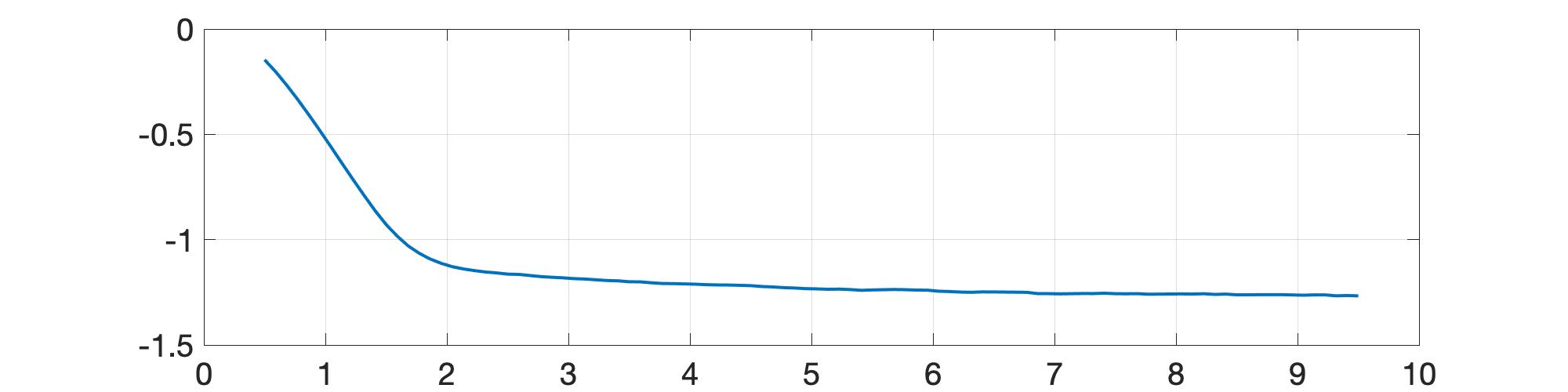
In Figure 3, we verify that when the arms are iid Bernoulli, KL-UCB produces regret distribution tails which are strictly lighter than truncated Cauchy, as predicted by Theorem 3.14.

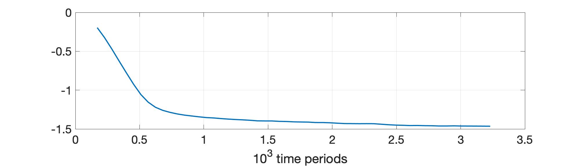
In Figure 4, we demonstrate the trade-off between the amount of UCB exploration (in Algorithm 1) and the resulting exponent of the regret distribution tail, as established in (41) and described in Remark 5.5.

In Figure 5, we demonstrate that the poor regret tail properties resulting from mis-specification of the serial dependence structure of the rewards can be overcome by aiming for a lighter regret tail using Algorithm 1. Here, we use the same AR(1) setup that is illustrated in Figure 2. As discussed in the first paragraph of Remark 5.12, here we do not have upper bounds on regret tail probabilities (only lower bounds in (37)), and thus there are no provable robustness guarantees. However, we show empirically in Figure 5 that aiming for a lighter regret tail still provides robustness to mis-specification in this setting. The $\frac{1+\beta_{0}}{1-\beta_{0}}$ factor in Figure 5 is taken from the lower bound in (37), which we essentially confirm to be tight here.

Figure 1: Plot of $\log\mathbb{P}_{\nu\pi}(N_{2}(T)\geq 0.8T)/\log(T)$ vs $T$. Environment $\nu=(N(0.1,\sigma_{0}^{2}),N(0,\sigma_{0}^{2}))$. Algorithm $\pi$ is KL-UCB for iid unit-variance Gaussian rewards. The curves correspond to the cases $\sigma_{0}^{2}=1,1.5,\dots,4$, as indicated by the legend. The curves asymptote to $-1/\sigma_{0}^{2}$ in each case, which agrees with Corollary 4.2 and (32).

Figure 2: Plot of $\log\mathbb{P}_{\nu\pi}(N_{2}(T)\geq 0.8T)/\log(T)$ vs $T$. Environment $\nu$ consists of two Gaussian AR(1) processes with common AR coefficient $\beta_{0}$, and equilibrium distributions $(N(0.1,1),N(0,1))$. Algorithm $\pi$ is KL-UCB for iid unit-variance Gaussian rewards. The curves correspond to the cases $\beta_{0}=0,0.15,\dots,0.9$, as indicated by the legend. The curves approximately asymptote to $-(1-\beta_{0})/(1+\beta_{0})$, which agrees with the lower bound in Corollary 4.7 and (37).

Figure 3: Plot of $\log\mathbb{P}_{\nu\pi}(N_{2}(T)>x)/\log(x)$ vs $x$ for $x\in[0.05T,0.95T]$ (with time horizon $T$ fixed). Environment $\nu=(\text{Ber}(q),\text{Ber}(0.4))$. Algorithm $\pi$ is KL-UCB for iid Bernoulli rewards. Top: $q=0.475$, $T=10^{4}$; Middle: $q=0.5$, $T=5\times 10^{3}$; Bottom: $q=0.525$, $T=3.4\times 10^{3}$. Each curve asymptotes to $\lim_{z\downarrow 0}d_{P}(z,q)/d_{P}(z,0.4)$ (with values $-1.26$ (top), $-1.36$ (middle), $-1.46$ (bottom)), as specified by Theorem 3.14 and (10).

Figure 4: Plot of $\log\mathbb{P}_{\nu\pi}(N_{2}(T)>x)/\log(x)$ vs $x$ for $x\in[0.05T,0.95T]$, with fixed time horizon $T=7\times 10^{3}$. Environment $\nu=(N(0.1,1),N(0,1))$. $\pi$ is Algorithm 1 with KL divergence $d_{P}$ between unit-variance Gaussian distributions, and we aim for a regret tail exponent of $-(1+b)$. The curves correspond to the cases $b=0,0.25,0.5,0.75$, as indicated by the legend. As predicted by (41), the curves asymptote to $-1$, $-1.25$, $-1.5$, $-1.75$.

Figure 5: Plot of $\log\mathbb{P}_{\nu\pi}(N_{2}(T)>x)/\log(x)$ vs $x$ for $x\in[0.05T,0.95T]$, with fixed time horizon $T=10^{4}$. Environment $\nu$ consists of two Gaussian AR(1) processes with common AR coefficient $\beta_{0}$, and equilibrium distributions $(N(0.1,1),N(0,1))$. $\pi$ is Algorithm 1 with KL divergence $d_{P}$ between unit-variance Gaussian distributions, and $1+b=1.1\cdot\frac{1+\beta_{0}}{1-\beta_{0}}$ (to aim for a regret tail exponent of $\approx-1.1$ in each case of $\beta_{0}$). The curves correspond to the cases $\beta_{0}=0,0.15,0.3,0.45$, as indicated by the legend. All curves asymptote to (slightly less than) $-1.1$, as desired.

8 Proofs for Section 3.1

For the proofs in Appendix 8, we will work with the natural parameterization of the exponential family in (1):

$$P_{\theta}(dx)=\exp\left(\theta\cdot x-\Lambda_{P}(\theta)\right)P(dx),\quad\theta\in\Theta_{P}.$$ (78)

Then the KL divergence between distributions $P_{\theta_{1}}$ and $P_{\theta_{2}}$ has the expression:

$$D(P_{\theta_{1}}\>\lVert\>P_{\theta_{2}})=\Lambda_{P}(\theta_{2})-\Lambda_{P}(\theta_{1})-\Lambda_{P}^{\prime}(\theta_{1})\cdot(\theta_{2}-\theta_{1}).$$ (79)

Proof 8.1

Proof of Lemma 3.3. First of all, the definition of discrimination equivalence as expressed in (6) for the exponential family with base distribution $P$ parameterized by mean (as in (1)) is equivalent to the following statement for the same exponential family with natural parameterization (as in (78)). For any $\theta_{1},\theta_{2}\in\Theta_{P}$ with $\theta_{1}>\theta_{2}$,

$$\inf_{\theta\in\Theta_{P}\,:\,\theta<\theta_{2}}\frac{D(P_{\theta}\>\lVert\>P_{\theta_{1}})}{D(P_{\theta}\>\lVert\>P_{\theta_{2}})}=1.$$ (80)

We first show the forward direction, that (80) implies (9). Suppose $\inf\Theta_{P}>-\infty$. Note that (80) implies that for any fixed $\theta_{0}>\inf\Theta_{P}$,

$$\lim_{\theta\downarrow\inf\Theta_{P}}D(P_{\theta}\>\lVert\>P_{\theta_{0}})=\lim_{\theta\downarrow\inf\Theta_{P}}\Lambda_{P}(\theta_{0})-\Lambda_{P}(\theta)-\Lambda_{P}^{\prime}(\theta)\cdot(\theta_{0}-\theta)=\infty.$$

Then taking $\theta_{0}$ arbitrarily close to $\inf\Theta_{P}$, we must have

$$\lim_{\theta\downarrow\inf\Theta_{P}}\Lambda_{P}(\theta)+\epsilon\Lambda_{P}^{\prime}(\theta)=-\infty$$ (81)

for any $\epsilon>0$. Because $\inf\Theta_{P}>-\infty$, (81) implies that

$$\lim_{\theta\downarrow\inf\Theta_{P}}\Lambda_{P}^{\prime}(\theta)=-\infty,$$ (82)

since $\Lambda_{P}$ is strictly convex and $\Lambda_{P}^{\prime}$ is strictly increasing on $\Theta_{P}$. Since

$$\lim_{\theta\downarrow\inf\Theta_{P}}\Lambda_{P}(\theta)>-\infty,$$

(81)-(82) imply that

$$\lim_{\theta\downarrow\inf\Theta_{P}}\left|\frac{\Lambda_{P}(\theta)}{\Lambda_{P}^{\prime}(\theta)}\right|=0.$$

So for any $\theta_{1},\theta_{2}$ fixed with $\theta_{1}>\theta_{2}>\inf\Theta_{P}$, we have

$$\lim_{\theta\downarrow\inf\Theta_{P}}\frac{D(P_{\theta}\>\lVert\>P_{\theta_{1}})}{D(P_{\theta}\>\lVert\>P_{\theta_{2}})}=\lim_{\theta\downarrow\inf\Theta_{P}}\frac{\Lambda_{P}^{\prime}(\theta)\cdot(\theta_{1}-\theta)}{\Lambda_{P}^{\prime}(\theta)\cdot(\theta_{2}-\theta)}=\frac{\theta_{1}-\inf\Theta_{P}}{\theta_{2}-\inf\Theta_{P}}>1,$$

which contradicts (80) if $\inf\Theta_{P}>-\infty$. Hence, it must be that $\inf\Theta_{P}=-\infty$.

Now suppose that

$$\lim_{\theta\to-\infty}\theta\Lambda_{P}^{\prime}(\theta)-\Lambda_{P}(\theta)<\infty.$$ (83)

Again, consider two the possible cases:

1. $\lim_{\theta\to-\infty}\Lambda_{P}^{\prime}(\theta)=-\infty$

2. $\lim_{\theta\to-\infty}\Lambda_{P}^{\prime}(\theta)>-\infty$.

In the first case, (80) cannot hold because (83) implies (for $\theta_{1}>\theta_{2}$):

$$\lim_{\theta\to-\infty}\frac{D(P_{\theta}\>\lVert\>P_{\theta_{1}})}{D(P_{\theta}\>\lVert\>P_{\theta_{2}})}=\lim_{\theta\to-\infty}\frac{\Lambda_{P}^{\prime}(\theta)\theta_{1}}{\Lambda_{P}^{\prime}(\theta)\theta_{2}}=\frac{\theta_{1}}{\theta_{2}}\neq 1.$$

In the second case, (80) cannot hold because (83) then implies that $\lim_{\theta\to-\infty}D(P_{\theta}\>\lVert\>P_{\theta_{0}})<\infty$ for any $\theta_{0}\in\Theta_{P}$. So it must be that

$$\lim_{\theta\to-\infty}\theta\Lambda_{P}^{\prime}(\theta)-\Lambda_{P}(\theta)=\infty.$$

Thus, the forward direction is established.

We now show the reverse direction, that (9) implies (80). For any $\theta_{1},\theta_{2}\in\Theta_{P}$ fixed with $\theta_{1}>\theta_{2}$,

$$\inf_{\theta\in\Theta_{P}\,:\,\theta<\theta_{2}}\frac{D(P_{\theta}\>\lVert\>P_{\theta_{1}})}{D(P_{\theta}\>\lVert\>P_{\theta_{2}})}\geq 1.$$

There are two possible cases:

1. $\lim_{\theta\to-\infty}\Lambda_{P}^{\prime}(\theta)=-\infty$

2. $\lim_{\theta\to-\infty}\Lambda_{P}^{\prime}(\theta)>-\infty$.

In the first case, note that for any fixed non-zero $\theta_{0}$, we have

$$\lim_{\theta\to-\infty}\frac{\theta_{0}\Lambda_{P}^{\prime}(\theta)}{\theta\Lambda_{P}^{\prime}(\theta)-\Lambda_{P}(\theta)}=\lim_{\theta\to-\infty}\frac{\theta_{0}}{\theta}=0.$$

And if $\theta_{0}=0$, then of course the same limit result holds. So (9) implies that

$$\lim_{\theta\to-\infty}\frac{D(P_{\theta}\>\lVert\>P_{\theta_{1}})}{D(P_{\theta}\>\lVert\>P_{\theta_{2}})}=\lim_{\theta\to-\infty}\frac{\theta\Lambda_{P}^{\prime}(\theta)-\Lambda_{P}(\theta)}{\theta\Lambda_{P}^{\prime}(\theta)-\Lambda_{P}(\theta)}=1.$$ (84)

In the second case, (9) directly implies (84). Thus, the reverse direction is established.

Proof 8.2

Proof of Proposition 3.4. Since $\inf\Theta_{P}=-\infty$ and the support of the distributions is unbounded to the left (i.e., there is always positive probability mass to the left of any point on the real line), as we send $\theta$ to $-\infty$, the mean $\mu(P_{\theta})=\Lambda_{P}^{\prime}(\theta)$ must also go to $-\infty$. By the definition of the convex conjugate $\Lambda_{P}^{*}$, we have for any $\theta\in\Theta_{P}$,

$$\Lambda_{P}^{*}(z)\geq\theta\cdot z-\Lambda_{P}(\theta),$$

which implies for $\theta<0$ that

$$\lim_{z\to-\infty}\Lambda_{P}^{*}(z)=\infty.$$

Also note that for any $\theta\in\Theta_{P}$,

$$\Lambda_{P}^{*}(\Lambda_{P}^{\prime}(\theta))=\theta\cdot\Lambda_{P}^{\prime}(\theta)-\Lambda_{P}(\theta).$$

So using $\lim_{\theta\to-\infty}\Lambda_{P}^{\prime}(\theta)=-\infty$ yields the desired result.

Proof 8.3

Proof of Proposition 3.5. Let $X$ be a random variable with distribution $P$. We first address the case where the distributions assign no mass to the (finite) infimum of their support, which we denote by $L$. For some $l>L$ with $l-L$ small (which will be made precise later), we have by the definition of convex conjugation:

$$\Lambda_{P}^{*}(l) =\sup_{\theta\in\Theta_{P}}\bigl{(}\theta\cdot l-\log\mathbb{E}[\exp(\theta X)]\bigr{)}$$

$$=-\log\left(\inf_{\theta\in\Theta_{P}}\mathbb{E}[\exp(\theta(X-l))]\right).$$ (85)

Let us decompose via:

$$\mathbb{E}[\exp(\theta(X-l))]=\mathbb{E}[\exp(\theta(X-l));X\geq l]+\mathbb{E}[\exp(\theta(X-l));X<l].$$ (86)

For $\theta<0$, the first term on the right side of (86) can be bounded via:

$$0\leq\mathbb{E}[\exp(\theta(X-l));X\geq l]\leq\exp(\left|\theta(l-L)\right|)\cdot\mathbb{E}[\exp(\theta(X-L))],$$ (87)

while the second term can be bounded via:

$$0\leq\mathbb{E}[\exp(\theta(X-l));X<l]\leq\exp(\left|\theta(l-L)\right|)\cdot\mathbb{P}(X<l).$$ (88)

Now for any $\epsilon>0$, set $\theta=-1/\epsilon$ and $l-L=\epsilon$, so that $\exp(\left|\theta(l-L)\right|)=\exp(1)$ in (87)-(88). Since $X\geq L$ with probability one and $X$ always has continuous CDF in a neighborhood of $L$, by the bounded convergence theorem, $\lim_{\theta\to-\infty}\mathbb{E}[\exp(\theta(X-L))]=0$. Moreover, $\lim_{l\downarrow L}\mathbb{P}(X<l)=0$. So the upper bounds in (87)-(88) can be made arbitrarily small by taking (the just defined) $\epsilon>0$ to be sufficiently small. Therefore, we have shown that

$$\lim_{l\downarrow L}\inf_{\theta\in\Theta_{P}}\mathbb{E}[\exp(\theta(X-l))]=0,$$

which, by (85), translates into

$$\lim_{l\downarrow L}\Lambda_{P}^{*}(l)=\infty.$$

Since

$$\lim_{\theta\to-\infty}\Lambda_{P}^{\prime}(\theta)=L,$$

we have

$$\lim_{\theta\to-\infty}\Lambda_{P}^{*}(\Lambda_{P}^{\prime}(\theta))=\infty,$$ (89)

which is the equivalent representation for (9).

In the case where there is strictly positive mass on $L$, note that if we take $l>L$ with $l$ sufficiently close to $L$, then the infimum in $\inf_{\theta\in\Theta_{P}}\mathbb{E}[\exp(\theta(X-l))]$ from (85) is achieved with $\theta<0$. (This is completely trivial if $\mathbb{P}(X=L)=\mathbb{P}(X<l)$ for $l>L$ with $l$ sufficiently close to $L$.) So it suffices to simply consider $\theta<0$. Then for $l>L$ with $l$ sufficiently close to $L$, we have the lower bounds:

$$\inf_{\theta\in\Theta_{P}}\mathbb{E}[\exp(\theta(X-l))] \geq\inf_{\theta<0}\mathbb{E}[\exp(\theta(X-l));X=L]$$

$$=\inf_{\theta<0}\exp(\theta(L-l))\cdot\mathbb{P}(X=L)$$

$$=\mathbb{P}(X=L).$$

Therefore, we have shown that

$$\liminf_{l\downarrow L}\inf_{\theta\in\Theta_{P}}\mathbb{E}[\exp(\theta(X-l))]\geq\mathbb{P}(X=L),$$

which, by (85), translates into

$$\limsup_{l\downarrow L}\Lambda_{P}^{*}(l)\leq-\log\mathbb{P}(X=L)<\infty,$$

since $\mathbb{P}(X=L)>0$ by assumption. So although

$$\lim_{\theta\to-\infty}\Lambda_{P}^{\prime}(\theta)=L,$$

unlike in the case of continuous distributions, where we ended up with (89), here we have

$$\limsup_{\theta\to-\infty}\Lambda_{P}^{*}(\Lambda_{P}^{\prime}(\theta))<\infty.$$

9 Proofs for Section 3.2

Proof 9.1

Proof of Proposition 3.13.

Let $i$ be any sub-optimal arm. From the lower bounds in (55) in the proof of Theorem 3.2, there exists $a>0$ such that for all $x\in[\log^{1+\gamma}(T),(1-\gamma)T]$ and $T$ sufficiently large,

$$T^{-a} \leq\mathbb{P}_{\nu\pi}(N_{i}(T)>(1-\gamma)T)$$

$$\leq\mathbb{P}_{\nu\pi}(N_{i}(T)>x).$$

Thus,

$$0 \leq\mathbb{P}_{\nu\pi}\left(\left|\widehat{\mu}_{i}(T)-\mu_{i}\right|>\epsilon\mid N_{i}(T)>x\right)$$

$$\leq\frac{\mathbb{P}_{\nu\pi}\left(\left|\widehat{\mu}_{i}(T)-\mu_{i}\right|>\epsilon,\;N_{i}(T)>\log^{1+\gamma}(T)\right)}{\mathbb{P}_{\nu\pi}\left(N_{i}(T)>(1-\gamma)T\right)}$$

$$\leq T^{a}\cdot 2\exp\left(-\log^{1+\gamma}(T)\cdot(\Lambda^{*}_{P^{\mu_{i}}}(\mu_{i}+\epsilon)\wedge\Lambda^{*}_{P^{\mu_{i}}}(\mu_{i}-\epsilon))\right),$$

where to obtain the last inequality, we use Cramér’s Theorem (see, for example, Theorem 2.2.3 on page 27 of Dembo and Zeitouni (1998)) to upper bound the numerator. So $\mathbb{P}_{\nu\pi}\left(\left|\widehat{\mu}_{i}(T)-\mu_{i}\right|>\epsilon\mid N_{i}(T)>x\right)\to 0$ uniformly for $x\in[\log^{1+\gamma}(T),(1-\gamma)T]$ as $T\to\infty$, which yields the desired result.

10 Proofs for Section 3.3

Proof 10.1

Verification of (70) in Proof of Theorem 3.14. With the natural parameterization of an exponential family $P_{\theta}$, $\theta\in\Theta_{P}$, as in (78), with KL divergence as in (79), we have:

$$\frac{d}{d\theta}D(P_{\theta}\>\lVert\>P_{\theta_{0}})=-\Lambda_{P}^{\prime\prime}(\theta)(\theta_{0}-\theta).$$

Denote $\theta_{1}:=\theta_{P}(\mu_{1})$ and $\theta_{2}:=\theta_{P}(\mu_{2})$ (with $\theta_{P}(\cdot)$ as defined in the parameterization by mean in (1)), so that $\theta_{2}<\theta_{1}$. Let $\epsilon>0$ such that $\theta_{2}+\epsilon<\theta_{1}$. Then,

$$\frac{d}{d\theta}\frac{D(P_{\theta}\>\lVert\>P_{\theta_{1}})}{D(P_{\theta}\>\lVert\>P_{\theta_{2}+\epsilon})}=\frac{\Lambda_{P}^{\prime\prime}(\theta)}{D(P_{\theta}\>\lVert\>P_{\theta_{2}+\epsilon})^{2}}\left(\underbrace{D(P_{\theta}\>\lVert\>P_{\theta_{1}})(\theta_{2}+\epsilon-\theta)-D(P_{\theta}\>\lVert\>P_{\theta_{2}+\epsilon})(\theta_{1}-\theta)}_{:=\xi(\theta)}\right).$$

Note that $\xi(\theta_{2}+\epsilon)=0$ and $\xi^{\prime}(\theta)=D(P_{\theta}\>\lVert\>P_{\theta_{2}+\epsilon})-D(P_{\theta}\>\lVert\>P_{\theta_{1}})$ for $\theta<\theta_{2}+\epsilon$. So $\xi^{\prime}(\theta)<0$, and thus $\xi(\theta)>0$ for $\theta<\theta_{2}+\epsilon$. From this, together with the fact that $\Lambda_{P}^{\prime\prime}(\theta)\geq 0$ for all $\theta$, we conclude that $\theta\mapsto D(P_{\theta}\>\lVert\>P_{\theta_{1}})/D(P_{\theta}\>\lVert\>P_{\theta_{2}+\epsilon})$ is monotone increasing for $\theta<\theta_{2}+\epsilon$.

Let $\delta>0$ such that $\mu_{2}+\delta<\mu_{1}$. Since $z\mapsto\theta_{P}(z)$ is monotone increasing, $z\mapsto d_{P}(z,\mu_{1})/d_{P}(z,\mu_{2}+\delta)$ must also be monotone increasing for $z<\mu_{2}+\delta$. So for any $\delta>0$,

$$\inf_{z<\mu_{2}+\delta}\frac{d_{P}(z,\mu_{1})}{d_{P}(z,\mu_{2}+\delta)}=\inf_{z<\mu_{2}}\frac{d_{P}(z,\mu_{1})}{d_{P}(z,\mu_{2}+\delta)}.$$

Since for $z<\mu_{2}$, $\delta\mapsto d_{P}(z,\mu_{1})/d_{P}(z,\mu_{2}+\delta)$ is monotone decreasing, it must also be that $\delta\mapsto\inf_{z<\mu_{2}}d_{P}(z,\mu_{1})/d_{P}(z,\mu_{2}+\delta)$ is monotone decreasing. Therefore,

$$\lim_{\delta\downarrow 0}\inf_{z<\mu_{2}}\frac{d_{P}(z,\mu_{1})}{d_{P}(z,\mu_{2}+\delta)}=\sup_{\delta>0}\inf_{z<\mu_{2}}\frac{d_{P}(z,\mu_{1})}{d_{P}(z,\mu_{2}+\delta)}.$$

Finally, since both $z\mapsto d_{P}(z,\mu_{1})/d_{P}(z,\mu_{2}+\delta)$ and $\delta\mapsto d_{P}(z,\mu_{1})/d_{P}(z,\mu_{2}+\delta)$ are monotone, and thus are both quasi-convex and quasi-concave, Sion’s Minimax Theorem yields:

$$\sup_{\delta>0}\inf_{z<\mu_{2}}\frac{d_{P}(z,\mu_{1})}{d_{P}(z,\mu_{2}+\delta)}=\inf_{z<\mu_{2}}\sup_{\delta>0}\frac{d_{P}(z,\mu_{1})}{d_{P}(z,\mu_{2}+\delta)}=\inf_{z<\mu_{2}}\frac{d_{P}(z,\mu_{1})}{d_{P}(z,\mu_{2})}.$$

11 Proofs for Section 3.4

The proof of Lemma 11.1 is a simplification of the proof of Proposition 3.17.

Lemma 11.1

Under the assumptions of Theorem 3.16, for any environment $\nu=(P_{1},\dots,P_{K})\in\mathcal{M}^{K}$ and each sub-optimal arm $i$, we have $N_{i}(T)\to\infty$ in $\mathbb{P}_{\nu\pi}$-probability as $T\to\infty$.

Proof 11.2

Proof of Lemma 11.1. Suppose the conclusion is false for some environment $\widetilde{\nu}=(\widetilde{P}_{1},P_{2},\dots,P_{K})\in\mathcal{M}^{K}$. Without loss of generality, suppose arm 1 is sub-optimal in $\widetilde{\nu}$ and there exists $m>0$, $\epsilon>0$ and a deterministic sequence of times $T_{n}\uparrow\infty$ such that

$$\mathbb{P}_{\widetilde{\nu}\pi}\left(N_{1}(T_{n})\leq m\right)\geq\epsilon.$$ (90)

Denote the event in (90) by $\mathcal{A}_{n}^{\prime}$. Consider another environment $\nu=(P_{1},P_{2},\dots,P_{K})\in\mathcal{M}^{K}$ where arm 1 is optimal (with all other arms being the same as in $\widetilde{\nu}$). Pick $L>0$ large enough so that

$$\mathbb{P}_{\widetilde{\nu}\pi}\left(\forall\;l=1,\dots,m:\frac{1}{l}\sum_{t=1}^{l}\log\frac{dP_{1}}{d\widetilde{P}_{1}}(X_{1}(t))\geq-D(\widetilde{P}_{1}\>\lVert\>P_{1})-L\right)\geq 1-\epsilon/2.$$ (91)

Define

$$\mathcal{B}_{n}^{\prime} =\biggl{\{}\frac{1}{N_{1}(T_{n})}\sum_{t=1}^{N_{1}(T_{n})}\log\frac{dP_{1}}{d\widetilde{P}_{1}}(X_{1}(t))\geq-D(\widetilde{P}_{1}\>\lVert\>P_{1})-L\biggr{\}}.$$

Following the same steps from (23)-(25) but with $\mathcal{A}_{n}^{\prime}$, $\mathcal{B}_{n}^{\prime}$ in the place of $\mathcal{A}_{n}$, $\mathcal{B}_{n}$, respectively,

$$\mathbb{P}_{\nu\pi}(\exists\;i\neq 1:N_{i}(T_{n})>T_{n}/(2K))\geq\mathbb{P}_{\widetilde{\nu}\pi}(\mathcal{A}_{n}^{\prime},\mathcal{B}_{n}^{\prime})\cdot\exp\left(-\left(D(\widetilde{P}_{1}\>\lVert\>P_{1})+L\right)m\right).$$

From (90) and (91), we have $\mathbb{P}_{\widetilde{\nu}\pi}(\mathcal{A}_{n}^{\prime},\mathcal{B}_{n}^{\prime})\geq\epsilon/2$ for all $n$. This violates the $\mathcal{M}$-consistency of $\pi$, and thus (90) cannot be true.

12 Proofs for Section 4.1

Proof 12.1

Proof of Proposition 4.1.

The proof of the lower bound part of (31) follows from Theorem 4.5 (which uses Proposition 4.4). To establish the upper bound part of (31), we can use the same proof of Theorem 3.14; see Section 6.2. Without loss of generality, suppose that $\mu(Q_{1})>\mu(Q_{2})>\dots>\mu(Q_{K})$ (i.e., $r(i)=i$ for all $i\in[K]$). So the only thing that needs to be checked is the analog of (70):

$$\lim_{\delta\downarrow 0}\inf_{z<\mu(Q_{2})+\delta}\frac{d_{Q_{1}}(z,\mu(Q_{1}))}{d_{P}(z,\mu(Q_{2})+\delta)}=\inf_{z<\mu(Q_{2})}\frac{d_{Q_{1}}(z,\mu(Q_{1}))}{d_{P}(z,\mu(Q_{2}))}.$$ (92)

(Below, we check (92) for $Q_{1}$ and $Q_{2}$. The same arguments apply for the other combinations of $Q_{i}$, $i\geq 3$ and $Q_{j}$, $j\leq i-1$.) First, there exists a fixed $\eta>0$ (depending on $Q_{1}$ and $Q_{2}$) such that for all $\delta>0$ sufficiently small, we have both:

$$\inf_{z<\mu(Q_{2})}\frac{d_{Q_{1}}(z,\mu(Q_{1}))}{d_{P}(z,\mu(Q_{2}))} =\inf_{z<\mu(Q_{2})-\eta}\frac{d_{Q_{1}}(z,\mu(Q_{1}))}{d_{P}(z,\mu(Q_{2}))},$$ (93)

$$\inf_{z<\mu(Q_{2})+\delta}\frac{d_{Q_{1}}(z,\mu(Q_{1}))}{d_{P}(z,\mu(Q_{2})+\delta)} =\inf_{z<\mu(Q_{2})-\eta}\frac{d_{Q_{1}}(z,\mu(Q_{1}))}{d_{P}(z,\mu(Q_{2})+\delta)}.$$ (94)

Note that

$$z\mapsto\frac{d_{P}(z,\mu(Q_{2}))}{d_{P}(z,\mu(Q_{2})+\delta)}$$

is monotone decreasing for $z<\mu(P_{2})$, which we deduce from the verification of (70) in proof of Theorem 3.14 in Appendix 10. Also, we have:

$$\lim_{\delta\downarrow 0}\sup_{z<\mu(Q_{2})-\eta}\frac{d_{P}(z,\mu(Q_{2}))}{d_{P}(z,\mu(P_{2})+\delta)} =\sup_{\delta>0}\sup_{z<\mu(Q_{2})-\eta}\frac{d_{P}(z,\mu(Q_{2}))}{d_{P}(z,\mu(Q_{2})+\delta)}=1,$$

$$\lim_{\delta\downarrow 0}\frac{d_{P}(\mu(Q_{2})-\eta,\mu(Q_{2}))}{d_{P}(\mu(Q_{2})-\eta,\mu(Q_{2})+\delta)} =1.$$

Therefore, we have uniform convergence for $z<\mu(P_{2})-\eta$:

$$\lim_{\delta\downarrow 0}\sup_{z<\mu(Q_{2})-\eta}\left|\frac{d_{P}(z,\mu(Q_{2}))}{d_{P}(z,\mu(Q_{2})+\delta)}-1\right|=0.$$ (95)

For any $\epsilon\in(0,1)$, using (95), we have for sufficiently small $\delta>0$:

$$(1-\epsilon)\inf_{z<\mu(Q_{2})-\eta}\frac{d_{Q_{1}}(z,\mu(Q_{1}))}{d_{P}(z,\mu(Q_{2}))} \leq\inf_{z<\mu(Q_{2})-\eta}\frac{d_{Q_{1}}(z,\mu(Q_{1}))}{d_{P}(z,\mu(Q_{2})+\delta)}\cdot\frac{d_{P}(z,\mu(Q_{2}))}{d_{P}(z,\mu(Q_{2}))}$$

$$\leq(1+\epsilon)\inf_{z<\mu(Q_{2})-\eta}\frac{d_{Q_{1}}(z,\mu(Q_{1}))}{d_{P}(z,\mu(Q_{2}))}.$$

Sending $\delta\downarrow 0$, followed by $\epsilon\downarrow 0$, and then using (93)-(94), we obtain (92).

Proof 12.2

Proof of Corollary 4.2.

Let $\nu$ consist of two Gaussian reward distributions with variance $\sigma_{0}^{2}$, and $\mu_{1}$ and $\mu_{2}$ as the means for arms 1 and 2, respectively. Without loss of generality, suppose that $\mu_{1}>\mu_{2}$ (i.e., $r(i)=i$ for $i=1,2$). The proof of the lower bound part of (31) follows from Theorem 4.5 (which uses Proposition 4.4). The upper bound part:

$$\limsup_{T\to\infty}\frac{\log\mathbb{P}_{\nu\pi}(N_{2}(T)>\log^{1+\gamma}(T))}{\log(\log^{1+\gamma}(T))}\leq-\frac{\sigma^{2}}{\sigma_{0}^{2}},$$ (96)

actually follows from the proof of the upper bound part of Theorem 3.14. In the Gaussian setting, the proof is substantially simpler, and so for future reference, we provide it below. The uniformity over $x$ follows by the monotonicity of $x\mapsto\log\mathbb{P}_{\nu\pi}(N_{2}(T)>x)/\log(x)$ for fixed $T$ and $x>1$.

Proof 12.3

Verification of (96) in Proof of Corollary 4.2. Let $x_{T}=\left\lfloor\log^{1+\gamma}(T)\right\rfloor$ with fixed $\gamma\in(0,1)$. Let $\Delta=\mu_{1}-\mu_{2}>0$. As in the proof of Theorem 3.14, we have:

$$\mathbb{P}_{\nu\pi}\left(N_{2}(T)>x_{T}\right)$$

$$\leq\mathbb{P}_{\nu\pi}\left(\exists\;t\in(\tau_{2}(x_{T}),T]\;\;\;\text{s.t.}\;\;\;\widehat{\mu}_{1}(t-1)+\sqrt{\frac{2\sigma^{2}\log(t-1)}{N_{1}(t-1)}}\leq\widehat{\mu}_{2}(t-1)+\sqrt{\frac{2\sigma^{2}\log(t-1)}{N_{2}(t-1)}}\right)$$

$$\leq\mathbb{P}_{\nu\pi}\left(\exists\;t\in(x_{T},T]\;\;\;\text{s.t.}\;\;\;\widehat{\mu}_{1}(t-1)+\sqrt{\frac{2\sigma^{2}\log(x_{T})}{N_{1}(t-1)}}\leq\widehat{\mu}_{2}(\tau_{2}(x_{T}))+\sqrt{\frac{2\sigma^{2}\log(T)}{x_{T}}}\right)$$

$$\leq\mathbb{P}_{\nu\pi}\left(\exists\;t\in(x_{T},T]\;\;\;\text{s.t.}\;\;\;\widehat{\mu}_{1}(t-1)+\sqrt{\frac{2\sigma^{2}\log(x_{T})}{N_{1}(t-1)}}\leq\mu_{2}+\frac{\Delta}{2}\right)$$ (97)

$$\quad+\mathbb{P}_{\nu\pi}\left(\widehat{\mu}_{2}(\tau_{2}(x_{T}))+\sqrt{\frac{2\sigma^{2}\log(T)}{x_{T}}}>\mu_{2}+\frac{\Delta}{2}\right).$$ (98)

For the term in (97), we have

$$(\ref{term1}) =\mathbb{P}_{\nu\pi}\left(\exists\;t\in(x_{T},T]\;\;\;\text{s.t.}\;\;\;\widehat{\mu}_{1}(t-1)+\sqrt{\frac{2\sigma^{2}\log(x_{T})}{N_{1}(t-1)}}\leq\mu_{1}-\frac{\Delta}{2}\right)$$

$$\leq\sum_{m=1}^{\infty}\mathbb{P}_{\nu\pi}\left(\frac{1}{m}\sum_{l=1}^{m}X_{1}(l)\leq\mu_{1}-\sqrt{\frac{2\sigma^{2}\log(x_{T})}{m}}-\frac{\Delta}{2}\right)$$ (99)

$$\leq\sum_{m=1}^{\infty}\exp\left(-\frac{m}{2\sigma_{0}^{2}}\left(\sqrt{\frac{2\sigma^{2}\log(x_{T})}{m}}+\frac{\Delta}{2}\right)^{2}\right)$$ (100)

$$=x_{T}^{-\sigma^{2}/\sigma_{0}^{2}}\cdot\sum_{m=1}^{\infty}\exp\left(-\frac{\sqrt{m\sigma^{2}\log(x_{T})}\Delta}{\sqrt{2}\sigma_{0}^{2}}-\frac{m\Delta^{2}}{8\sigma_{0}^{2}}\right)$$

$$\leq x_{T}^{-\sigma^{2}/\sigma_{0}^{2}}\cdot\sum_{m=1}^{\infty}\exp\left(-\frac{\sqrt{m}\sigma\Delta}{\sqrt{2}\sigma_{0}^{2}}-\frac{m\Delta^{2}}{8\sigma_{0}^{2}}\right)\qquad\quad(\text{for }T\geq 16),$$ (101)

where to obtain (99), we have used a union bound over all possible values of $N_{1}(t)$, $t\geq 1$, and to obtain (100), we have used a large deviations upper bound.

For the term in (98), we have for sufficiently large $T$,

$$\sqrt{\frac{2\sigma^{2}\log(T)}{x_{T}}}<\frac{\Delta}{4}.$$

So for sufficiently large $T$,

$$(\ref{term2}) \leq\mathbb{P}_{\nu\pi}\left(\frac{1}{x_{T}}\sum_{t=1}^{x_{T}}X_{2}(t)>\mu_{2}+\frac{\Delta}{4}\right)$$

$$\leq\exp\left(-x_{T}\cdot\frac{\Delta^{2}}{32\sigma_{0}^{2}}\right),$$ (102)

where to obtain (102), we have used a large deviations upper bound.

Putting together (97), (101) and (98), (102), we have established the desired result:

$$\limsup_{T\to\infty}\frac{\log\mathbb{P}_{\nu\pi}\left(N_{2}(T)>x_{T}\right)}{\log(x_{T})}\leq-\frac{\sigma^{2}}{\sigma_{0}^{2}}.$$

13 Proofs for Section 4.2

Proof 13.1

Proof of Proposition 4.4.

This proof is an extension and simplification of Propositions 7-8 of Cowan and Katehakis (2019).

We restrict our attention to sample paths $\omega$ belonging to

$$\left\{\omega:\lim_{n\to\infty}\frac{1}{n}\sum_{t=1}^{n}X_{i}(t)=\mu_{i},\;i\in[K]\right\}.$$ (103)

Without loss of generality, suppose that arm $1$ is the unique optimal arm, i.e., $\mu_{1}>\max_{i\geq 2}\mu_{i}$. Here, we define the KL-UCB index for arm $i$ at time $t+1$ via:

$$U_{i}(t)=\sup\left\{z\in\mathcal{I}_{P}:d_{P}(\widehat{\mu}_{i}(t),z)\leq\frac{\log(t)}{N_{i}(t)}\right\},$$ (104)

where, as defined previously, $\widehat{\mu}_{i}(t)=\frac{1}{N_{i}(t)}\sum_{s=1}^{N_{i}(t)}X_{i}(s)$.

We begin with the upper bound part of the proof. Consider sub-optimal arm $i\geq 2$, and let $\delta\in(0,(\mu_{1}-\mu_{i})/2)$. We have

$$N_{i}(T) =1+\sum_{t=K}^{T-1}\mathbb{I}\left({A(t+1)=i,\;U_{i}(t)\geq\mu_{1}-\delta,\;\widehat{\mu}_{i}(t)\leq\mu_{i}+\delta}\right)$$ (105)

$$\quad\;\;\;+\sum_{t=K}^{T-1}\mathbb{I}\left({A(t+1)=i,\;U_{i}(t)\geq\mu_{1}-\delta,\;\widehat{\mu}_{i}(t)>\mu_{i}+\delta}\right)$$ (106)

$$\quad\;\;\;+\sum_{t=K}^{T-1}\mathbb{I}\left({A(t+1)=i,\;U_{i}(t)<\mu_{1}-\delta}\right),$$ (107)

where $A(t)$ is the arm sampled by the algorithm at time $t$.

The first sum is upper bounded via:

$$(\ref{sum1}) \leq\sum_{t=K}^{T-1}\mathbb{I}\left({A(t+1)=i,\;d_{P}(\mu_{i}+\delta,\mu_{1}-\delta)\leq\frac{\log(t)}{N_{i}(t)}}\right)$$ (108)

$$\leq\sum_{t=K}^{T-1}\mathbb{I}\left({A(t+1)=i,\;N_{i}(t)\leq\frac{\log(T)}{d_{P}(\mu_{i}+\delta,\mu_{1}-\delta)}}\right)$$

$$\leq\frac{\log(T)}{d_{P}(\mu_{i}+\delta,\mu_{1}-\delta)}+1.$$ (109)

The bound in (108) holds due to the events $U_{i}(t)\geq\mu_{1}-\delta$ and $\widehat{\mu}_{i}(t)\leq\mu_{i}+\delta$ and the definition of the index in (104).

The second sum is upper bounded via:

$$(\ref{sum2})\leq\sum_{t=K}^{\infty}\mathbb{I}\left({A(t+1)=i,\;\widehat{\mu}_{i}(t)>\mu_{i}+\delta}\right).$$ (110)

On sample paths in (103), the indicators on the right side of (110) can equal $1$ for at most finitely many $t$. (For each $1$ in the sum, arm $i$ is played an additional time and an additional sample incorporated into $\widehat{\mu}_{i}(t)$.)

The third sum is upper bounded via:

$$(\ref{sum3}) \leq\sum_{t=K}^{\infty}\mathbb{I}\left({A(t+1)=i,\;U_{1}(t)\leq U_{i}(t)<\mu_{1}-\delta}\right)$$

$$\leq\sum_{t=K}^{\infty}\mathbb{I}\left({U_{1}(t)<\mu_{1}-\delta}\right).$$ (111)

On sample paths in (103), the indicators on the right side of (111) can equal $1$ for at most finitely many $t$. (As $t\to\infty$, either $N_{1}(t)$ increases to infinity or remains finite. In the first case, $\widehat{\mu}_{1}(t)\to\mu_{1}$, and so for $t$ sufficiently large, $U_{1}(t)\geq\widehat{\mu}_{1}(t)>\mu_{1}-\delta/2$. In the second case, $\log(t)$ in (104) increases without bound, and so $U_{1}(t)$ also increases without bound, with $U_{1}(t)>\mu_{1}$ for all $t$ sufficiently large.)

Putting together (109)-(111), and sending $T\to\infty$ followed by $\delta\downarrow 0$, we have for each sub-optimal arm $i\geq 2$,

$$\limsup_{T\to\infty}\frac{N_{i}(T)}{\log(T)}\leq\frac{1}{d_{P}(\mu_{i},\mu_{1})}.$$ (112)

Therefore, for the optimal arm $1$,

$$\lim_{T\to\infty}\frac{N_{1}(T)}{T}=1,$$ (113)

which, by the form of the index in (104), then implies:

$$\lim_{t\to\infty}U_{1}(t)=\mu_{1}.$$ (114)

Then, (113) and (114) imply that for each sub-optimal arm $i\geq 2$,

$$\lim_{T\to\infty}N_{i}(T)=\infty.$$ (115)

(If (115) is not true for some sub-optimal arm $j$, then since the term $\log(t)$ grows without bound in the index (104), we would eventually have $U_{j}(t)>\mu_{1}+\epsilon>U_{1}(t)$ for some $\epsilon>0$ and all $t$ sufficiently large, thereby contradicting (113).)

We now develop the lower bound parts of the proof. As defined previously, for any positive integer $m$, we use $\tau_{1}(m)$ to denote the time of the $m$-th play of arm $1$. So for each sub-optimal arm $i\geq 2$,

$$U_{1}(\tau_{1}(m)-1)>U_{i}(\tau_{1}(m)-1).$$ (116)

Let $\delta>0$. We have for $m$ sufficiently large,

$$\max_{t\in[\tau_{1}(m),\tau_{1}(m+1)]}\frac{\log(t)}{N_{i}(t)} \leq\frac{\log(\tau_{1}(m+1))}{N_{i}(\tau_{1}(m)-1)}$$

$$=\frac{\log(\tau_{1}(m+1))}{\log(\tau_{1}(m)-1)}\frac{\log(\tau_{1}(m)-1)}{N_{i}(\tau_{1}(m)-1)}$$

$$\leq(1+\delta)\frac{\log(\tau_{1}(m)-1)}{N_{i}(\tau_{1}(m)-1)}$$ (117)

$$\leq(1+\delta)d_{P}(\mu_{i}-\delta,U_{i}(\tau_{1}(m)-1))$$ (118)

$$\leq(1+\delta)d_{P}(\mu_{i}-\delta,U_{1}(\tau_{1}(m)-1))$$ (119)

$$\leq(1+\delta)d_{P}(\mu_{i}-\delta,\mu_{1}+\delta).$$ (120)

Note that (117) is due to (113), (118) is due to $\lim_{t\to\infty}\widehat{\mu}_{i}(t)=\mu_{i}$ for each sub-optimal arm $i\geq 2$ and the form of the index in (104), (119) is due to (116), and (120) is due to (114). From (120), we see that

$$\liminf_{T\to\infty}\frac{N_{i}(T)}{\log(T)}\geq\frac{1}{d_{P}(\mu_{i},\mu_{1})},$$

which together with (112), completes the proof.

Proof 13.2

Proof of Theorem 4.5.

Without loss of generality, suppose that the long-run average rewards (in the sense of (33)) for arms $1,2,\dots,K$ within the environment $\nu$ satisfy $\mkern 1.5mu\overline{\mkern-1.5mu\Lambda\mkern-1.5mu}\mkern 1.5mu_{1}^{\prime}(0)>\mkern 1.5mu\overline{\mkern-1.5mu\Lambda\mkern-1.5mu}\mkern 1.5mu_{2}^{\prime}(0)>\dots>\mkern 1.5mu\overline{\mkern-1.5mu\Lambda\mkern-1.5mu}\mkern 1.5mu_{K}^{\prime}(0)$ (i.e., $r(i)=i$ for all $i\in[K]$). Consider any sub-optimal arm $i\geq 2$. Let $\widetilde{\nu}$ be an alternative environment where the reward distribution structure remains the same for arms $i,i+1,\dots,K$. However, for arm $j\leq i-1$ in the environment $\widetilde{\nu}$, let the distribution of $\sum_{t=1}^{n}X_{j}(t)$ for each $n\geq 1$ be

$$Q_{j}^{n}(dx;\theta_{j})=\exp\left(\theta_{j}\cdot x-n\mkern 1.5mu\overline{\mkern-1.5mu\Lambda\mkern-1.5mu}\mkern 1.5mu_{j}^{n}(\theta_{j})\right)Q_{j}^{n}(dx),$$

where $Q_{j}^{n}(dx)$ is the original distribution for $\sum_{t=1}^{n}X_{j}(t)$ in the environment $\nu$. Moreover, let $\theta_{j}\in\mkern 1.5mu\overline{\mkern-1.5mu\Theta\mkern-1.5mu}\mkern 1.5mu_{j}$ such that $\mkern 1.5mu\overline{\mkern-1.5mu\Lambda\mkern-1.5mu}\mkern 1.5mu_{j}^{\prime}(\theta_{j})<\mkern 1.5mu\overline{\mkern-1.5mu\Lambda\mkern-1.5mu}\mkern 1.5mu_{i}^{\prime}(0)$ (note that $\theta_{j}<0$). (If this is not possible, then the infimum on the right side of (35) is empty, and the lower bound is $-\infty$.) So in the environment $\widetilde{\nu}$, arm $i$ yields the highest long-run average rewards compared to all other arms.

Let $\delta>0$, and define the events:

$$\mathcal{A}_{T}=\left\{\left|\frac{N_{j}(T)}{\log(T)}-\frac{1}{d_{P}(\mkern 1.5mu\overline{\mkern-1.5mu\Lambda\mkern-1.5mu}\mkern 1.5mu_{j}^{\prime}(\theta_{j}),\mkern 1.5mu\overline{\mkern-1.5mu\Lambda\mkern-1.5mu}\mkern 1.5mu_{i}^{\prime}(0))}\right|\leq\delta,\;\forall\;j\leq i-1\right\}$$

$$\qquad\;\;\cap\left\{\left|\frac{N_{j}(T)}{\log(T)}-\frac{1}{d_{P}(\mkern 1.5mu\overline{\mkern-1.5mu\Lambda\mkern-1.5mu}\mkern 1.5mu_{j}^{\prime}(0),\mkern 1.5mu\overline{\mkern-1.5mu\Lambda\mkern-1.5mu}\mkern 1.5mu_{i}^{\prime}(0))}\right|\leq\delta,\;\forall\;j\geq i+1\right\}$$

$$\mathcal{B}_{T}=\left\{\left|\widehat{\mu}_{j}(T)-\mkern 1.5mu\overline{\mkern-1.5mu\Lambda\mkern-1.5mu}\mkern 1.5mu_{j}^{\prime}(\theta_{j}))\right|\leq\delta,\;\forall\;j\leq i-1\right\}.$$

Following steps analogous to (51)-(53) in the proof of Theorem 3.2,

$$\mathbb{P}_{\nu\pi}(N_{i}(T)>(1-\gamma)T)$$

$$=\mathbb{E}_{\widetilde{\nu}\pi}\left[\mathbb{I}\left({N_{i}(T)>(1-\gamma)T}\right)\exp\left(\sum_{j=1}^{i-1}\left(-\theta_{j}\cdot\sum_{t=1}^{N_{j}(T)}X_{j}(t)+N_{j}(T)\cdot\mkern 1.5mu\overline{\mkern-1.5mu\Lambda\mkern-1.5mu}\mkern 1.5mu_{j}^{N_{j}(T)}(\theta_{j})\right)\right)\right]$$ (121)

$$\geq\mathbb{E}_{\widetilde{\nu}\pi}\left[\mathbb{I}\left({\mathcal{A}_{T},\mathcal{B}_{T}}\right)\exp\left(\sum_{j=1}^{i-1}\Bigl{(}-\theta_{j}\cdot\widehat{\mu}_{j}(T)+\mkern 1.5mu\overline{\mkern-1.5mu\Lambda\mkern-1.5mu}\mkern 1.5mu_{j}^{N_{j}(T)}(\theta_{j})\Bigr{)}N_{j}(T)\right)\right]$$ (122)

$$\geq\mathbb{E}_{\widetilde{\nu}\pi}\left[\mathbb{I}\left({\mathcal{A}_{T},\mathcal{B}_{T}}\right)\exp\left(\sum_{j=1}^{i-1}\Bigl{(}-\theta_{j}\cdot\left(\mkern 1.5mu\overline{\mkern-1.5mu\Lambda\mkern-1.5mu}\mkern 1.5mu_{j}^{\prime}(\theta_{j})-\delta\right)+\mkern 1.5mu\overline{\mkern-1.5mu\Lambda\mkern-1.5mu}\mkern 1.5mu_{j}(\theta_{j})-\delta\Bigr{)}N_{j}(T)\right)\right]$$ (123)

$$=\mathbb{E}_{\widetilde{\nu}\pi}\left[\mathbb{I}\left({\mathcal{A}_{T},\mathcal{B}_{T}}\right)\exp\left(-\sum_{j=1}^{i-1}\Bigl{(}\mkern 1.5mu\overline{\mkern-1.5mu\Lambda\mkern-1.5mu}\mkern 1.5mu_{j}^{*}(\mkern 1.5mu\overline{\mkern-1.5mu\Lambda\mkern-1.5mu}\mkern 1.5mu_{j}^{\prime}(\theta_{j}))+\delta(1-\theta_{j})\Bigr{)}N_{j}(T)\right)\right]$$ (124)

$$\geq\mathbb{P}_{\widetilde{\nu}\pi}(\mathcal{A}_{T},\mathcal{B}_{T})\cdot\exp\left(-\sum_{j=1}^{i-1}\Bigl{(}\mkern 1.5mu\overline{\mkern-1.5mu\Lambda\mkern-1.5mu}\mkern 1.5mu_{j}^{*}(\mkern 1.5mu\overline{\mkern-1.5mu\Lambda\mkern-1.5mu}\mkern 1.5mu_{j}^{\prime}(\theta_{j}))+\delta(1-\theta_{j})\Bigr{)}\left(\frac{1}{d_{P}(\mkern 1.5mu\overline{\mkern-1.5mu\Lambda\mkern-1.5mu}\mkern 1.5mu_{j}^{\prime}(\theta_{j}),\mkern 1.5mu\overline{\mkern-1.5mu\Lambda\mkern-1.5mu}\mkern 1.5mu_{i}^{\prime}(0))}+\delta\right)\log(T)\right).$$ (125)

In (121), we have performed a change-of-measure from environment $\nu$ to $\widetilde{\nu}$. In (122), we use the fact that $\{N_{i}(T)>(1-\gamma)T\}\supset\mathcal{A}_{T}$ for sufficiently large $T$. We have used the event $\mathcal{B}_{T}$ in (123), and the relevant identity for the convex conjugates $\mkern 1.5mu\overline{\mkern-1.5mu\Lambda\mkern-1.5mu}\mkern 1.5mu_{j}^{*}$ in (124). We have used the event $\mathcal{A}_{T}$ in (125). We also note that $\lim_{T\to\infty}\mathbb{P}_{\widetilde{\nu}\pi}(\mathcal{A}_{T},\mathcal{B}_{T})=1$. In environment $\widetilde{\nu}$, $\lim_{T\to\infty}\mathbb{P}_{\widetilde{\nu}\pi}(\mathcal{A}_{T})=1$ is due to the $\mathcal{M}_{P}$-pathwise convergence property of the algorithm $\pi$, as in (34). And $\lim_{T\to\infty}\mathbb{P}_{\widetilde{\nu}\pi}(\mathcal{B}_{T})=1$ is due to the same result for $\mathcal{A}_{T}$, together with the sample mean WLLN that comes from Assumptions 4.2-4.2 (using the upper bound part of the Gärtner-Ellis Theorem; for details, see Lemma 3.2.5 of Bucklew (2004)). From (125), taking logs and dividing by $\log(T)$, and sending $T\to\infty$ followed by $\delta\downarrow 0$, we obtain:

$$\liminf_{T\to\infty}\frac{\log\mathbb{P}_{\nu\pi}(N_{i}(T)>(1-\gamma)T)}{\log(T)}\geq-\sum_{j=1}^{i-1}\frac{\mkern 1.5mu\overline{\mkern-1.5mu\Lambda\mkern-1.5mu}\mkern 1.5mu_{j}^{*}(\mkern 1.5mu\overline{\mkern-1.5mu\Lambda\mkern-1.5mu}\mkern 1.5mu_{j}^{\prime}(\theta_{j}))}{d_{P}(\mkern 1.5mu\overline{\mkern-1.5mu\Lambda\mkern-1.5mu}\mkern 1.5mu_{j}^{\prime}(\theta_{j}),\mkern 1.5mu\overline{\mkern-1.5mu\Lambda\mkern-1.5mu}\mkern 1.5mu_{i}^{\prime}(0))}.$$

This holds for any $\theta_{j}\in\mkern 1.5mu\overline{\mkern-1.5mu\Theta\mkern-1.5mu}\mkern 1.5mu_{j}$, $j\leq i-1$ such that $\mkern 1.5mu\overline{\mkern-1.5mu\Lambda\mkern-1.5mu}\mkern 1.5mu_{j}^{\prime}(\theta_{j})<\mkern 1.5mu\overline{\mkern-1.5mu\Lambda\mkern-1.5mu}\mkern 1.5mu_{i}^{\prime}(0)$. Under Assumptions 4.2-4.2, each $\mkern 1.5mu\overline{\mkern-1.5mu\Lambda\mkern-1.5mu}\mkern 1.5mu_{j}^{\prime}$ is an invertible mapping between $\mkern 1.5mu\overline{\mkern-1.5mu\Theta\mkern-1.5mu}\mkern 1.5mu_{j}$ and $\overline{\mathcal{I}}_{j}$ (see Theorem 26.5 of Rockafellar (1970)). Thus,

$$\liminf_{T\to\infty}\frac{\log\mathbb{P}_{\nu\pi}(N_{i}(T)>(1-\gamma)T)}{\log(T)}\geq-\sum_{j=1}^{i-1}\inf_{z\in\overline{\mathcal{I}}_{j}\,:\,z<\mkern 1.5mu\overline{\mkern-1.5mu\Lambda\mkern-1.5mu}\mkern 1.5mu_{i}^{\prime}(0)}\frac{\mkern 1.5mu\overline{\mkern-1.5mu\Lambda\mkern-1.5mu}\mkern 1.5mu_{j}^{*}(z)}{d_{P}(z,\mkern 1.5mu\overline{\mkern-1.5mu\Lambda\mkern-1.5mu}\mkern 1.5mu_{i}^{\prime}(0))}.$$

The conclusion (35) holds with the infimum over $B_{\gamma}(T)=[\log^{1+\gamma}(T),(1-\gamma)T]$ due to $x\mapsto\log\mathbb{P}_{\nu\pi}(N_{i}(T)>x)/\log(x)$ being monotone decreasing for $x\in B_{\gamma}(T)$, with $T$ fixed.

References

- Agrawal (1995) Agrawal R (1995) Sample mean based index policies with regret for the multi-armed bandit problem. Advances in Applied Probability 27(4):1054–1078.
- Ashutosh et al. (2021) Ashutosh K, Nair J, Kagrecha A, Jagannathan K (2021) Bandit algorithms: letting go of logarithmic regret for statistical robustness. International Conference on Artificial Intelligence and Statistics .
- Audibert et al. (2009) Audibert J, Munos R, Szepesvári C (2009) Exploration–exploitation tradeoff using variance estimates in multi-armed bandits. Theoretical Computer Science 410(19):1876–1902.
- Auer et al. (2002) Auer P, Cesa-Bianchi N, Fischer P (2002) Finite-time analysis of the multiarmed bandit problem. Machine Learning 47:235–256.
- Baudry et al. (2021) Baudry D, Gautron R, Kaufmann E, Maillard O (2021) Optimal Thompson sampling strategies for support-aware CVaR bandits. International Conference on Machine Learning .
- Bucklew (2004) Bucklew J (2004) Introduction to Rare Event Simulation (Springer).
- Burnetas and Katehakis (1996) Burnetas A, Katehakis M (1996) Optimal adaptive policies for sequential allocation problems. Advances in Applied Mathematics 17(2):122–142.
- Cappé et al. (2013) Cappé O, Garivier A, Maillard O, Munos R, Stoltz G (2013) Kullback-Leibler upper confidence bounds for optimal sequential allocation. The Annals of Statistics 41(3):1516–1541.
- Cassel et al. (2018) Cassel A, Mannor S, Zeevi A (2018) A general approach to multi-armed bandits under risk criteria. Conference on Learning Theory .
- Cowan and Katehakis (2019) Cowan W, Katehakis M (2019) Exploration–exploitation policies with almost sure, arbitrarily slow growing asymptotic regret. Probability in the Engineering and Informational Sciences 34(3):406–428.
- Dembo and Zeitouni (1998) Dembo A, Zeitouni O (1998) Large Deviations Techniques and Applications (Springer-Verlag).
- Fan and Glynn (2022) Fan L, Glynn P (2022) The typical behavior of bandit algorithms. Working Paper .
- Galichet et al. (2013) Galichet N, Sebag M, Teytaud O (2013) Exploration vs exploitation vs safety: risk-aware multi-armed bandits. Asian Conference on Machine Learning 245–260.
- Garivier and Cappé (2011) Garivier A, Cappé O (2011) The KL-UCB algorithm for bounded stochastic bandits and beyond. Conference on Learning Theory 359–376.
- Garivier et al. (2019) Garivier A, Menard P, Stoltz G (2019) Explore first, exploit next: the true shape of regret in bandit problems. Mathematics of Operations Research 44(2):377–399.
- Kaufmann et al. (2016) Kaufmann E, Cappé O, Garivier A (2016) On the complexity of best-arm identification in multi-armed bandit models. Journal of Machine Learning Research 17(1):1–42.
- Khajonchotpanya et al. (2021) Khajonchotpanya N, Xue Y, Rujeerapaiboon N (2021) A revised approach for risk-averse multi-armed bandits under CVaR criterion. Operations Research Letters 49(4):465–472.
- Kontoyiannis and Meyn (2003) Kontoyiannis I, Meyn S (2003) Spectral theory and limit theorems for geometrically ergodic Markov processes. The Annals of Applied Probability 13(1):304–362.
- Korda et al. (2013) Korda N, Kaufmann E, Munos R (2013) Thompson sampling for 1-dimensional exponential family bandits. NeurIPS 26.
- Lai (1987) Lai T (1987) Adaptive treatment allocation and the multi-armed bandit problem. The Annals of Statistics 15(3):1091–1114.
- Lai and Robbins (1985) Lai T, Robbins H (1985) Asymptotically efficient adaptive allocation rules. Advances in Applied Mathematics 6(1):4–22.
- Lattimore and Szepesvári (2020) Lattimore T, Szepesvári C (2020) Bandit Algorithms (Cambridge University Press).
- Maillard (2013) Maillard O (2013) Robust risk-averse stochastic multi-armed bandits. International Conference on Algorithmic Learning Theory 218–233.
- Maillard et al. (2011) Maillard O, Munos R, Stoltz G (2011) A finite-time analysis of multi-armed bandits problems with Kullback-Leibler divergences. Conference on Learning Theory 497–514.
- Miller (1961) Miller H (1961) A Convexity Property in the Theory of Random Variables Defined on a Finite Markov Chain. The Annals of Mathematical Statistics 32(4):1260–1270.
- Moulos and Anantharam (2019) Moulos V, Anantharam V (2019) Optimal Chernoff and Hoeffding bounds for finite state Markov chains. arXiv:1907.04467 .
- Prashanth et al. (2020) Prashanth L, Jagannathan K, Kolla R (2020) Concentration bounds for CVaR estimation: the cases of light-tailed and heavy-tailed distributions. International Conference on Machine Learning .
- Rockafellar (1970) Rockafellar R (1970) Convex Analysis (Princeton University Press).
- Rudin (1987) Rudin W (1987) Real and Complex Analysis (McGraw-Hill).
- Salomon and Audibert (2011) Salomon A, Audibert J (2011) Deviations of stochastic bandit regret. International Conference on Algorithmic Learning Theory 159–173.
- Sani et al. (2012) Sani A, Lazaric A, Munos R (2012) Risk-aversion in multi-armed bandits. Advances in Neural Information Processing Systems .
- Szorenyi et al. (2015) Szorenyi B, Busa-Fekete R, Weng P, Hullermeier E (2015) Qualitative multi-armed bandits: a quantile-based approach. International Conference on Machine Learning .
- Tamkin et al. (2019) Tamkin A, Keramati R, Dann C, Brunskill E (2019) Distributionally-aware exploration for CVaR bandits. Advances in Neural Information Processing Systems .
- Thompson (1933) Thompson W (1933) On the likelihood that one unknown probability exceeds another in view of the evidence of two samples. Biometrika 25(3):285–294.
- Vakili and Zhao (2016) Vakili S, Zhao Q (2016) Risk-averse multi-armed bandit problems under mean-variance measure. IEEE Journal of Selected Topics in Signal Processing 10(6):1093–1111.
- Zhu and Tan (2020) Zhu Q, Tan V (2020) Thompson sampling for mean-variance bandits. International Conference on Machine Learning .
- Zimin et al. (2014) Zimin A, Ibsen-Jensen R, Chatterjee K (2014) Generalized risk-aversion in stochastic multi-armed bandits. arXiv:1405.0833 .