Metastability of Ising and Potts Models without External Fields in Large Volumes at Low Temperatures

Abstract.

In this article, we investigate the energy landscape and metastable behavior of the Ising and Potts models on two-dimensional square or hexagonal lattices in the low temperature regime, especially in the absence of an external magnetic field. The energy landscape of these models without an external field is known to have a huge and complex saddle structure between ground states. In the small volume regime where the lattice is finite and fixed, the aforementioned complicated saddle structure has been successfully analyzed in [20] for two or three dimensional square lattices when the inverse temperature tends to infinity. In this article, we consider the large volume regime where the size of the lattice grows to infinity. We first establish an asymptotically sharp threshold such that the ground states are metastable if and only if the inverse temperature is larger than the threshold in a suitable sense. Then, we carry out a detailed analysis of the energy landscape and rigorously establish the Eyring–Kramers formula when the inverse temperature is sufficiently larger than the previously mentioned sharp threshold. The proof relies on detailed characterization of dead-ends appearing in the vicinity of optimal transitions between ground states and on combinatorial estimation of the number of configurations lying on a certain energy level.

1. Introduction

Metastability is a ubiquitous phenomenon that occurs when a stochastic system has multiple locally stable sets. It occurs in a wide class of models in statistical mechanics such as interacting particle systems [5, 10], spin systems [6, 14, 24], small random perturbations of dynamical systems [15], and models in numerical simulations such as the kinetic Monte Carlo [17] and stochastic gradient descent method [16]. We refer to the bibliography of the listed references for more comprehensive literature. We also refer to monographs such as [11, 26] and references therein.

Ising and Potts model

In this article, we are interested in the Ising/Potts model defined on either a square or hexagonal lattice $\Lambda_{L}$ with side length $L\in\mathbb{N}$ under the periodic boundary condition. For $q\geq 2$, denote by $\{1,\,2,\,\dots,\,q\}$ the set of spins so that we can get a spin configuration by distributing spins at the vertices of lattice $\Lambda_{L}$. Then, the Ising/Potts model refers to the Gibbs measure on the space of spin configurations associated with a certain form of Hamiltonian function (cf. (2.3)) at inverse temperature $\beta$. In particular, the models with $q=2$ and $q\geq 3$ are called the Ising and Potts models, respectively. Henceforth, we assume that there is no external field acting on our Ising/Potts model.

Ground states and metastability

For $a\in\{1,\,\dots,\,q\}$, we denote by $\mathbf{a}$ the monochromatic spin configuration consisting only of spin $a$. Then, we can readily verify that the set of ground states associated with the Ising/Potts Hamiltonian is $\mathcal{S}=\{\mathbf{1},\,\dots,\,\mathbf{q}\}$ and hence the Gibbs measure is concentrated on the set $\mathcal{S}$ as the inverse temperature $\beta$ tends to infinity (i.e., as the temperature goes to $0$). Thus, we can expect that the associated heat-bath Glauber dynamics exhibits metastability when $\beta$ is sufficiently large, in the sense that the single-flip Glauber dynamics starting at a ground state $\mathbf{a}\in\mathcal{S}$ spends a very long time in a neighborhood of $\mathbf{a}$ before making a transition to another ground state. Such a metastable transition is one of the primary concerns of the study of metastability and we are specifically interested in the accurate quantification of the mean of the metastable transition time. Such a precise estimate of the mean transition time is called the Eyring–Kramers formula and establishing it requires deep understanding of the energy landscape, e.g., detailed saddle structure between ground states, associated with the Hamiltonian. The major difficulty confronted in the current article lies on the fact that the saddle structure includes a huge plateau with a large amount of dead-ends.

We remark that other important problems in the analysis of metastability include characterizing the typical transition paths and estimating the spectral gap or mixing time. We shall not pursue these questions in the current article and leave as future research program.

Metastability in small volumes at low temperatures

The energy landscape of the Ising/Potts model on two-dimensional square lattices in the small volume regime, i.e, when the side length $L$ of the lattice is large but fixed, was first analyzed in [22], where the energy barrier between ground states was exactly computed under periodic and open boundary conditions. Based on this result, the large deviation-type analysis of metastability in the low temperature regime, i.e., $\beta\rightarrow\infty$ regime, has been carried out via a robust pathwise approach-type method developed in [23]. This analysis has been extended in [7] where the authors provide more refined characterization of the optimal transition paths between ground states.

Finally, in the paper [20] by the authors of the present work, a complete characterization of the entire saddle structure has been carried out on fixed two or three dimensional square lattices with periodic or open boundary conditions. This level of detailed understanding of the energy landscape enables us to deduce the Eyring–Kramers formula in the very low temperature regime. By adopting the methodology developed in that article, metastability of the Blume–Capel model with zero external field and zero chemical potential has also been analyzed in [19].

Main results

In this article, we consider the Ising/Potts model in the large volume regime, i.e., the case when the side length $L$ grows to infinity. We analyze, at a highly accurate level, the energy landscape of the Ising/Potts model on the two-dimensional square or hexagonal lattice of side length $L$ with periodic boundary conditions.

Note that the Gibbs measure is concentrated on the set $\mathcal{S}$ of ground states if $L$ is fixed and $\beta$ is sufficiently large, since the entropy effect can be neglected in this regime and the energy is the only dominating factor. However, if we assume that $L$ and $\beta$ are both sufficiently large, we must consider the entropy effect and the competition between energy and entropy should be carefully quantified to determine whether the Gibbs measure is still concentrated on $\mathcal{S}$. This precise quantification of the entropy-energy competition is done in Theorem 3.2 where we establish a zero-one law-type result. More precisely, we demonstrate that there exists a constant $\gamma_{0}$ such that

$$\begin{cases}\text{if }\beta\geq\gamma\log L\text{ for }\gamma>\gamma_{0}\text{ then the Gibbs measure is concentrated on }\mathcal{S}\text{ and}\\ \text{if }\beta\leq\gamma\log L\text{ for }\gamma<\gamma_{0}\text{ then the Gibbs measure is concentrated on }\mathcal{S}^{c}\end{cases}$$

as $L\rightarrow\infty$, where $\gamma$ denotes a constant independent of $L$. Therefore, we find an interesting phase transition at the critical inverse temperature $\beta_{0}(L)=\gamma_{0}\log L$.

In view of the previous result, the sharp estimation of the mean of transition time between ground states provides the Eyring–Kramers formula only when we asymptotically have $\beta\geq\gamma\log L$ for some $\gamma>\gamma_{0}$. Indeed, we carry out the analysis of the energy landscape and establish the Eyring–Kramers formula under $\beta\geq\gamma\log L$, $\gamma>\gamma_{1}$ for some constant $\gamma_{1}$ which is larger than $\gamma_{0}$ due to technical reasons.

Challenges in the proof

For both square and hexagonal lattices with side length $L$ under periodic boundary conditions, it can be shown (cf. [22] for the square lattice and Theorem 3.1 of the present work for the hexagonal lattice) that the energy barrier between ground states is $2L+2$. In the small volume regime considered in [7, 20, 22], we can neglect all the configurations of energy larger than $2L+2$ since the number of such configurations is determined solely by $L$ (and hence fixed) and therefore, as $\beta\rightarrow\infty$, these configurations have exponentially negligible mass with respect to the Gibbs measure, compared to the configurations with energy less than or equal to $2L+2$ along which typical metastable transitions take place. However, for the models in the large volume regime, we are no longer able to neglect these configurations, as the number of such configurations also grows to infinity and hence the entropy plays a role. This is the first primary difficulty in the study of models in large volume when compared to the previous works; indeed, a subtle combinatorial estimation on the number of configurations on each energy level is required to overcome this difficulty.

We remark that the saddle structure for the Ising/Potts model without external field forms a huge and complex plateau. The saddle plateau consists of canonical configurations providing the main road in the course of metastable transition, and a large amount of dead-ends attached there. The analysis of canonical configurations is rather straightforward, but we need to fully understand the complex structure of the dead-ends in order to obtain quantitative results such as the Eyring–Kramers formula. In the two-dimensional square lattice, it is observed in [20] that the dead-ends are attached only at the edge part of the saddle plateau thanks to its special local geometry, and this feature allows us to avoid serious difficulties arising from the analysis of dead-ends. However, for other forms of general lattices, this miracle does not occur and the dead-ends are attached along the whole saddle plateau, so that they form a highly complicated maze structure.

We believe that our methodology for proving the Eyring–Kramers formula is robust against this dead-end structure, and to highlight this robustness we focus our proof on the hexagonal lattice, in which the dead-ends structure is indeed complex and emerges in the entire part of the saddle plateau. The dead-end analysis of the hexagonal lattice relies on the characterization of all the relevant configurations with energy around $2L+2$ (cf. Section 6) and a significant effort of the current article is devoted to completely understand this dead-end structure of the hexagonal lattice.

Remarks on the Ising/Potts model with non-zero external field

We conclude the introduction with some remarks on the Ising/Potts model with non-zero external field at very low temperatures. The metastability of this model has been thoroughly investigated during the last few decades, and it is interesting that the results are completely different from the zero external field models considered in [7, 20, 22] and the current article.

For the non-zero external field Ising model in small volume, the saddle structure of the metastable transition is characterized by appearance of the specific form of a critical droplet, and hence has a very sharp saddle structure, in contrast to the fact that the zero external field model has a huge saddle plateau. Such a characterization has been carried out in [24, 25] for the two-dimensional square lattice, in [6] for the three-dimensional square lattice, and in [1] for the two-dimensional hexagonal lattice. In the last work, it was also been observed that the local geometry of the hexagonal lattice induces additional difficulty in the analysis of dead-ends in the vicinity of the critical droplet. These results also imply the Eyring–Kramers formula via potential-theoretic arguments developed in [14]. The same result has been obtained recently in [8, 9] for the Potts model when the external field acts only on a single spin. An interesting open question is to analyze the energy landscape and verify the Eyring–Kramers formula when the external field acts on all $q$ spins. The main difficulty of the Potts model compared to the Ising model is the lack of monotonicity, which was crucially used in [24, 25] to analyze the typical transition path via a grand coupling.

For the model in large volume, it is verified in [12] that the formation of a critical droplet is still crucial in the transition in the Ising case. In that article, three regimes of metastable transitions were studied: formation of a critical droplet, formation of a supercritical droplet, and evolution of the droplet to a larger size. Typical trajectories for the metastable transition and the saddle structure have not been fully characterized yet, and it even remains unknown whether the saddle configuration contains either one or multiple critical droplets. Hence, the Eyring–Kramers formula remains an open question for this model.

2. Model

Before stating the main result of the current article, we rigorously introduce the model in the current section.

2.1. Spin systems

Lattices

In this article, we consider spin systems on large, finite two-dimensional lattices.

Fix a large positive integer $L\in\mathbb{N}$ and denote by $\Lambda_{L}^{\textup{sq}}$ and $\Lambda_{L}^{\textup{hex}}$ the square and hexagonal lattices (cf. Figure 2.1) of size $L$ with periodic boundary conditions. There is no ambiguity in the definition of $\Lambda_{L}^{\textup{sq}}$, but further explanation of $\Lambda_{L}^{\textup{hex}}$ is required. To define $\Lambda_{L}^{\textup{hex}}$, we first select $2L^{2}$ vertices from infinite hexagonal lattice as in Figure 2.1-(left). Then, we identify the points at the boundary naturally as illustrated in the figure. This setting will become intuitively clear when we introduce the dual lattice in the sequel.

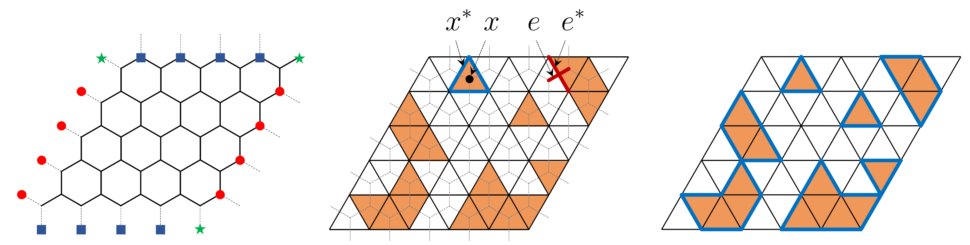
Figure 2.1. (Left) A hexagonal lattice $\Lambda=\Lambda_{5}^{\textup{hex}}$ with $2\times 5^{2}=50$ vertices which are the end points of bold edges. Under the periodic boundary condition, each vertex at the boundary highlighted by red circle (resp. blue square) is identified with another one with red circle (resp. blue square) at the same horizontal level (resp. same diagonal line with slope $\pi/3$). (Middle) The dual lattice $\Lambda^{*}$ of the hexagonal lattice which is a triangular lattice. The vertex $x$ of $\Lambda$ is identified with the triangular face $x^{*}$ (the one highlighted by blue bold boundary) in $\Lambda^{*}$. The edge $e$ of $\Lambda$ is identified with its dual edge $e^{*}$ of $\Lambda^{*}$. In this and the right figure, if the spin at a certain vertex is $1$ (resp. $2$), we paint the corresponding triangular face by white (resp. orange). Namely, in this figure we consider the Ising case $q=2$ and we have $\sigma(x)=2$. (Right) Edges in $\mathfrak{A}^{*}(\sigma)$ are denoted by blue bold edges, and hence $\mathfrak{A}^{*}(\sigma)$ is a collection of edges at the boundaries of the monochromatic clusters. Since the Hamiltonian of $\sigma$ can be computed as $|\mathfrak{A}^{*}(\sigma)|$, as we observed in (2.6), $H(\sigma)$ is just the sum of perimeters of the orange (or white, equivalently) clusters.

Spin configuration

We henceforth let $\Lambda=\Lambda_{L}^{\textup{sq}}$ or $\Lambda_{L}^{\textup{hex}}$. For an integer $q\geq 2$, define the set of spins as

$$\Omega=\Omega_{q}=\{1,\,2,\,\dots,\,q\}$$ (2.1)

and we assign a spin from $\Omega$ at each site (vertex) $x$ of $\Lambda$. The resulting object belonging to the space $\Omega^{\Lambda}$ is called a (spin) configuration. We write

$$\mathcal{X}=\mathcal{X}_{L}=\Omega^{\Lambda}$$ (2.2)

the space of spin configurations. We use the notation $\sigma=(\sigma(x))_{x\in\Lambda}$ to denote a spin configuration, i.e., an element of $\mathcal{X}$, where $\sigma(x)$ represents the spin at site $x\in\Lambda$.

Visualization via dual lattice

To visualize spin configurations, it is convenient to consider the dual lattice $\Lambda^{*}$ of $\Lambda$. If $\Lambda=\Lambda_{L}^{\textup{sq}}$, the dual lattice $\Lambda^{*}$ is again a periodic square lattice of side length $L$. On the other hand, if $\Lambda=\Lambda_{L}^{\textup{hex}}$, the dual lattice $\Lambda^{*}$ is a rhombus-shaped periodic triangular lattice with side length $L$ as in Figure 2.1-(middle). Note that the periodic boundary condition of the triangular lattice inherited from that of the hexagonal lattice simply identifies four boundaries of the rhombus in a routine way (as in $\mathbb{Z}_{L}^{2}$).

Since we can identify a site of $\Lambda$ with a face of $\Lambda^{*}$ containing it, we can regard the spins assigned at the sites of $\Lambda$ as those assigned to the faces of $\Lambda^{*}$. Thus, by assigning different colors to each set of spins, we can readily visualize the spin configurations on the dual lattice. For instance, in Figure 2.1-(middle, right), the triangles with white and orange colors correspond to the vertices of spins $1$ and $2$, respectively. This visualization is conceptually more convenient in analyzing the energy of spin configurations, as we explain in the next subsection.

2.2. Ising and Potts models

The Ising and Potts models are defined through a suitable probability distribution on the space $\mathcal{X}$ of spin configurations (cf. (2.2)). To define this, let us first define the Ising/Potts Hamiltonian $H:\mathcal{X}\rightarrow\mathbb{R}$ by

$$H(\sigma)=\sum_{x\sim y}\mathbf{1}\{\sigma(x)\neq\sigma(y)\}\;\;\;\;;\;\sigma\in\mathcal{X}\;,$$ (2.3)

where $x\sim y$ if and only if $x$ and $y$ are connected by an edge of the lattice $\Lambda$. We emphasize here that this definition of $H$ indicates that there is no external field acting on the Hamiltonian. Denote by $\mu_{\beta}(\cdot)$ the Gibbs measure on $\mathcal{X}$ associated with the Hamiltonian $H(\cdot)$ at the inverse temperature $\beta>0$, i.e.,

$$\mu_{\beta}(\sigma)=\frac{1}{Z_{\beta}}e^{-\beta H(\sigma)}\text{ for }\sigma\in\mathcal{X}\;,\;\;\;\text{where}\;\;\;\;Z_{\beta}=\sum_{\zeta\in\mathcal{X}}e^{-\beta H(\zeta)}\;.$$ (2.4)

The random spin configuration associated with the probability measure $\mu_{\beta}(\cdot)$ is called the Ising model if $q=2$ and the Potts model if $q\geq 3$.

Computing the Hamiltonian via dual lattice representation

We can identify an edge $e$ in $\Lambda$ with the unique edge $e^{*}$ in the dual lattice $\Lambda^{*}$ intersecting with $e$ (cf. Figure 2.1-(middle)), and we can identify each vertex $x$ in $\Lambda$ with the unique face $x^{*}$ in the dual lattice $\Lambda^{*}$ containing $x$. As we have mentioned in Section 2.1, we regard each spin in $\Omega=\{1,\,2,\,\dots,\,q\}$ as a color, so that each face $x^{*}$ in the dual lattice is painted by the color corresponding to the spin at $x$. Thus, we can identify $\sigma\in\mathcal{X}$ with a $q$-coloring on the faces of the dual lattice $\Lambda^{*}$. In this coloring representation of $\sigma$, each maximal monochromatic connected component is called a (monochromatic) cluster of $\sigma$.

We now explain a convenient formulation to understand the Hamiltonian of a spin configuration $\sigma\in\mathcal{X}$ with the setting explained above. We refer to Figure 2.1-(right) for an illustration. Define $\mathfrak{A}(\sigma)$ as the collection of edges $e=\{x,\,y\}$ in $\Lambda$ such that $\sigma(x)\neq\sigma(y)$. Then, define

$$\mathfrak{A}^{*}(\sigma)=\{e^{*}:e\in\mathfrak{A}(\sigma)\}\;,$$ (2.5)

so that by the definition of the Hamiltonian, we have

$$H(\sigma)=|\mathfrak{A}(\sigma)|=|\mathfrak{A}^{*}(\sigma)|\;.$$ (2.6)

The crucial observation is that the dual edge $e^{*}$ belongs to $\mathfrak{A}^{*}(\sigma)$ if and only if $e^{*}$ belongs to the boundary of a cluster of $\sigma$. Hence, as in Figure Figure 2.1-(right), we can readily compute the energy $H(\sigma)$ as

$$H(\sigma)=\frac{1}{2}\sum_{A^{*}:\text{ cluster of }\sigma}(\textup{perimeter of }A^{*})\;,$$ (2.7)

where the factor $\frac{1}{2}$ appears since each dual edge $e^{*}\in\mathfrak{A}^{*}(\sigma)$ belongs to the perimeter of exactly two clusters.

2.3. Heat-bath Glauber dynamics

We next introduce a heat-bath Glauber dynamics associated with the Gibbs measure $\mu_{\beta}(\cdot)$. We consider herein the continuous-time Metropolis–Hastings dynamics $\{\sigma_{\beta}(t)\}_{t\geq 0}$ on $\mathcal{X}$, whose jump rate from $\sigma\in\mathcal{X}$ to $\zeta\in\mathcal{X}$ is given by

$$c_{\beta}(\sigma,\,\zeta)=\begin{cases}e^{-\beta\max\{H(\zeta)-H(\sigma),\,0\}}&\text{if }\zeta=\sigma^{x,\,a}\neq\sigma\text{ for some }x\in\Lambda\text{ and }a\in\Omega\;,\\ 0&\text{otherwise},\end{cases}$$ (2.8)

where $\sigma^{x,\,a}\in\mathcal{X}$ denotes the configuration obtained from $\sigma$ by flipping the spin at site $x$ to $a$. This dynamics is standard in the study of metastability of the Ising/Potts model on lattices; see, e.g., [11, 24, 25] and references therein. For $\sigma,\,\zeta\in\mathcal{X}$, we write

$$\sigma\sim\zeta\;\;\;\;\text{if and only if}\;\;\;\;c_{\beta}(\sigma,\,\zeta)>0\;.$$ (2.9)

Note that the jump of dynamics $\sigma_{\beta}(\cdot)$ is available only through a single-spin flip. We will write $\mathbb{P}_{\sigma}^{\beta}$ the law of the Markov process $\sigma_{\beta}(\cdot)$ starting at $\sigma\in\mathcal{X}$, and write $\mathbb{E}_{\sigma}^{\beta}$ the corresponding expectation.

From the definitions of $\mu_{\beta}(\cdot)$ and $c_{\beta}(\cdot,\,\cdot)$, we can directly check the following so-called detailed balance condition:

$$\mu_{\beta}(\sigma)c_{\beta}(\sigma,\,\zeta)=\mu_{\beta}(\zeta)c_{\beta}(\zeta,\,\sigma)=\begin{cases}\min\{\mu_{\beta}(\sigma),\,\mu_{\beta}(\zeta)\}&\text{if }\sigma\sim\zeta\;,\\ 0&\text{otherwise.}\end{cases}$$ (2.10)

Hence, the Markov process $\sigma_{\beta}(\cdot)$ is reversible with respect to its invariant measure $\mu_{\beta}(\cdot)$.

3. Main Result

In this section, we explain the main results obtained in this article for the Ising/Potts model explained in the previous section. We assume hereafter that $L\geq 8$ to avoid unnecessary technical difficulties.

3.1. Hamiltonian and energy barrier

We first explain some results regarding the Hamiltonian $H(\cdot)$ of the Ising/Potts model.

Ground states

For each $a\in\Omega$, we denote by $\mathbf{a}\in\mathcal{X}$ the configuration of which all the spins are $a$, i.e., $\mathbf{a}(x)=a$ for all $x\in\Lambda$. Write

$$\mathcal{S}=\{\mathbf{1},\,\mathbf{2},\,\dots,\,\mathbf{q}\}\;\;\;\text{and}\;\;\;\mathcal{S}(A)=\{\mathbf{a}\in\mathcal{S}:a\in A\}$$

for each $A\subseteq\Omega$. Then, it is immediate from the definition that the Hamiltonian achieves its minimum $0$ exactly at the configurations belonging to $\mathcal{S}$, and therefore the set $\mathcal{S}$ denotes the collection of all ground states of the Ising/Potts model without external field.

Energy barrier

We first concern on the measurement of the energy barrier between the ground states. The energy barrier is a fundamental quantity in the investigation of the saddle structure between ground states. To define this, let a sequence of configurations $(\omega_{n})_{n=0}^{N}$ in $\mathcal{X}$ be a path of length $N$ if (cf. (2.9)),

$$\omega_{n}\sim\omega_{n+1}\;\;\;\;\text{for all }n\in\llbracket 0,\,N-1\rrbracket\;.$$ (3.1)

The path $(\omega_{n})_{n=0}^{N}$ is said to connect $\sigma$ and $\zeta$ if $\omega_{0}=\sigma$ and $\omega_{N}=\zeta$ or vice versa. The communication height between two configurations $\sigma,\,\zeta\in\mathcal{X}$ is defined as

$$\Phi(\sigma,\,\zeta)=\min_{(\omega_{n})_{n=0}^{N}\text{ connects }\sigma\text{ and }\zeta}\,\max_{n\in\llbracket 0,\,N\rrbracket}H(\omega_{n})\;.$$

Then, the energy barrier between ground states is defined as, for $\mathbf{a},\,\mathbf{b}\in\mathcal{S}$,

$$\Gamma=\Gamma_{\Lambda}=\Phi(\mathbf{a},\,\mathbf{b})\;,$$ (3.2)

where the value of $\Gamma$ is independent of the selection of $\mathbf{a},\,\mathbf{b}$ by the symmetry of the model.

Theorem 3.1.

For both $\Lambda=\Lambda_{L}^{\textup{sq}}$ and $\Lambda_{L}^{\textup{hex}}$, we have $\Gamma=2L+2$. Moreover, there is no valley of depth larger than $\Gamma$ in the sense that

$$\min_{\mathbf{s}\in\mathcal{S}}\Phi(\sigma,\,\mathbf{s})-H(\sigma)<\Gamma\;\;\;\;\text{for all }\sigma\in\mathcal{X}\setminus\mathcal{S}\;.$$

This theorem has been proven for square lattice in [22], and we prove this theorem for the hexagonal lattice in Section 6.

3.2. Concentration of Gibbs measure

We next investigate the Gibbs measure $\mu_{\beta}(\cdot)$. We can readily observe from definition that if $L$ is fixed and $\beta\rightarrow\infty$, the Gibbs measure $\mu_{\beta}(\cdot)$ is concentrated on the ground set $\mathcal{S}$. However, if we consider the large volume regime for which both $L$ and $\beta$ tends to $\infty$ together, the non-ground states can have non-negligible masses because of the entropy effect, that is, there are sufficiently many configurations with high energy that can dominate the mass of the ground states. By a careful combinatorial analysis carried out in Section 4, we can accurately quantify this competition between energy and entropy; consequently, we establish the zero-one law type result by finding a sharp threshold determining whether the Gibbs measure $\mu_{\beta}$ is concentrated on $\mathcal{S}$. Before explaining this result, we explicitly declare the regime that we consider.

Assumption.

The inverse temperature $\beta=\beta_{L}$ depends on $L$ and we consider the large-volume, low-temperature regime, in the sense that $\beta_{L}\rightarrow\infty$ as $L\rightarrow\infty$.

For sequences $(a_{L})_{L=1}^{\infty}$ and $(b_{L})_{L=1}^{\infty}$, we write $a_{L}\ll b_{L}$ if $\lim_{L\rightarrow\infty}a_{L}/b_{L}=0$ and write $a_{L}=o_{L}(1)$ if $\lim_{L\rightarrow\infty}a_{L}=0$. The following theorem will be proven in Section 4.

Theorem 3.2.

Let us define a constant $\gamma_{0}$ by

$$\gamma_{0}=\begin{cases}1/2&\text{for the square lattice},\\ 2/3&\text{for the hexagonal lattice}.\end{cases}$$ (3.3)

Then, the following estimates hold.

1. Suppose that $L^{\gamma_{0}}\ll e^{\beta}$. Then, we have (cf. (2.4)) $Z_{\beta}=q+o_{L}(1)$ and

   $$\mu_{\beta}(\mathcal{S})=1-o_{L}(1)\;.$$

2. On the other hand, suppose that $e^{\beta}\ll L^{\gamma_{0}}$. Then, we have

   $$\mu_{\beta}(\mathcal{S})=o_{L}(1)\;.$$

Henceforth, the constant $\gamma_{0}$ always refers to the one defined in (3.3). This theorem implies that a drastic change in the valley structure of the Gibbs measure $\mu_{\beta}$ occurs at $\beta/\log L=\gamma_{0}$. Namely, if $\beta/\log L\geq\gamma$ for some $\gamma>\gamma_{0}$, the ground states themselves form metastable sets, while if $\beta/\log L\leq\gamma$ for $\gamma<\gamma_{0}$, ground states are no longer metastable.

The second regime can be investigated further. Define, for each $i\geq 0$,

$$\mathcal{X}_{i}=\mathcal{X}_{i,\,L}=\{\sigma\in\mathcal{X}:H(\sigma)=i\}\;,$$ (3.4)

so that $\mathcal{X}_{0}=\mathcal{S}$ denotes the set of ground states. For any interval $I\subseteq\mathbb{R}$, we write

$$\mathcal{X}_{I}=\bigcup_{i\in I\cap\mathbb{Z}}\mathcal{X}_{i}\;.$$

Then, we have the following refinement of case (2) of Theorem 3.2 which will be proven in Section 4 as well.

Theorem 3.3.

Suppose that $e^{\beta}\ll L^{\gamma_{0}}$ and fix a constant $\alpha\in(0,\,1)$. Then, the following statements hold.

1. Suppose that $L^{\gamma_{0}(1-\alpha)}\ll e^{\beta}$. Then, for every $c>0$, we have

   $$\mu_{\beta}\big{(}\,\mathcal{X}_{[0,\,cL^{2\alpha}]}\,\big{)}=1-o_{L}(1)\;.$$

2. Suppose that $L^{\gamma_{0}(1-\alpha)}\gg e^{\beta}$. Then, for every $c>0$, we have

   $$\mu_{\beta}\big{(}\,\mathcal{X}_{[0,\,cL^{2\alpha}]}\,\big{)}=o_{L}(1)\;.$$

We can infer from Theorem 3.1 that the energetic valley $\mathcal{V}_{\mathbf{a}}$ containing each $\mathbf{a}\in\mathcal{S}$ should be the connected component of

$$\{\sigma\in\mathcal{X}:H(\sigma)<2L+2\}$$

containing $\mathbf{a}$, where the connectedness of a set $\mathcal{A}\subseteq\mathcal{X}$ here refers to the path-connectedness (cf. (3.1)). Since Theorem 3.3 implies that

$$\mu_{\beta}\big{(}\,\mathcal{X}_{[0,\,2L+1]}\,\big{)}=\begin{cases}1-o_{L}(1)&\text{if }L^{\gamma_{0}/2}\ll e^{\beta}\;,\\ o_{L}(1)&\text{if }L^{\gamma_{0}/2}\gg e^{\beta}\;,\end{cases}$$

we can conclude that the energetic valleys $\mathcal{V}_{\mathbf{a}}$ are indeed metastable valleys if $\beta/\log L\geq\gamma$ for some $\gamma>\frac{\gamma_{0}}{2}$. In contrast, if $\beta/\log L\leq\gamma$ for some $\gamma<\frac{\gamma_{0}}{2}$, the Gibbs measure is concentrated on the complement of these energetic valleys. Hence, in the latter regime (as long as $\beta$ is bigger than the critical temperature $\beta_{c}(q)=\log(1+\sqrt{q})$ of the Ising/Potts model [2]), we deduce that the metastable set must lie upon the configurations with higher energy; this is the onset in which the entropy starts to play a significant role.

3.3. Eyring–Kramers formula

We next concern on the dynamical metastable behavior exhibited by the Metropolis dynamics $\sigma_{\beta}(\cdot)$ defined in Section 2.3. If the invariant measure $\mu_{\beta}(\cdot)$ is concentrated on the set $\mathcal{S}$, we can expect that the process $\sigma_{\beta}(\cdot)$ starting at some $\mathbf{a}\in\mathcal{S}$ spends a sufficiently long time around $\mathbf{a}$ before making a transition to another ground state. This type of behavior is the signature of metastability of the process $\sigma_{\beta}(\cdot)$, and we are interested in its quantification. To explain this in more detail, we first define the hitting time of the set $\mathcal{A}\subseteq\mathcal{X}$ as

$$\tau_{\mathcal{A}}=\inf\{t\geq 0:\sigma_{\beta}(t)\in\mathcal{A}\}\;,$$

and simply write $\tau_{\{\sigma\}}=\tau_{\sigma}$. Then, we are primarily interested in the mean transition time of the form $\mathbb{E}_{\mathbf{a}}^{\beta}[\tau_{\mathcal{S}\setminus\{\mathbf{a}\}}]$ or $\mathbb{E}_{\mathbf{a}}^{\beta}[\tau_{\mathbf{b}}]$ denoting the expectation of the metastable transition from a ground state to another one, where $\mathbb{E}_{\mathbf{a}}^{\beta}$ is defined right after (2.9). These quantities are significant in the study of the metastable behavior because they are key notions explaining the amount of time required to observe a metastable transition and are closely related to the mixing time or spectral gap of the dynamics. The precise estimation of the mean transition time is called the Eyring–Kramers formula. The next main result of the current article is the following Eyring–Kramers formula for the Metropolis dynamics. Define a constant $\kappa_{0}$ by

$$\kappa_{0}=\begin{cases}1/8&\text{for the square lattice},\\ 1/12&\text{for the hexagonal lattice}.\end{cases}$$ (3.5)

Theorem 3.4 (Eyring–Kramers formula).

Suppose that $\beta=\beta_{L}$ satisfies $L^{3}\ll e^{\beta}$ for the square lattice and $L^{10}\ll e^{\beta}$ for the hexagonal lattice. Then, for all $\mathbf{a},\,\mathbf{b}\in\mathcal{S}$, we have

$$\mathbb{E}_{\mathbf{a}}^{\beta}\big{[}\,\tau_{\mathcal{S}\setminus\{\mathbf{a}\}}\,\big{]}=\frac{\kappa_{0}+o_{L}(1)}{q-1}e^{\Gamma\beta}\;\;\;\;\text{and}\;\;\;\;\mathbb{E}_{\mathbf{a}}^{\beta}\big{[}\,\tau_{\mathbf{b}}\,\big{]}=(\kappa_{0}+o_{L}(1))e^{\Gamma\beta}\;,$$ (3.6)

where $\Gamma=2L+2$ is the energy barrier obtained in Theorem 3.1.

The proof of this theorem is given in Sections 8 through 10 based on the comprehensive analysis of the saddle structure carried out in Sections 6 and 7.

Remark 3.5.

We conjecture that this result holds for all $\beta=\beta_{L}$ satisfying $L^{\gamma_{0}/2}\ll e^{\beta}$, under which the invariant measure is concentrated on the energetic valleys around ground states. The sub-optimality of the lower bound (of constant order) on $\beta$ owes to several technical issues arising in the proof (cf. Sections 9 and 10), and we guess that additional innovative ideas are required to get the optimal bound.

Remark 3.6.

The condition on $\beta$ is relatively tight ($L^{3}\ll e^{\beta}$) for the square lattice, whereas the condition for the hexagonal lattice is slightly loose ($L^{10}\ll e^{\beta}$). This is because the dead-end analysis is much more complicated for the hexagonal lattice owing to its complicated local geometry. It will be highlighted in Sections 6.2 and 6.3.

Remark 3.7.

One can also obtain the Markov chain convergence of the so-called trace process (cf. [3]) of the accelerated process $\{\sigma_{\beta}(e^{\Gamma\beta}t)\}_{t\geq 0}$ on the set $\mathcal{S}$ to the Markov process on $\mathcal{S}$ with uniform rate $r(\mathbf{a},\,\mathbf{b})=\frac{1}{\kappa_{0}}$ for all $\mathbf{a},\,\mathbf{b}\in\mathcal{S}$. Such a Markov chain model reduction of the metastable behavior is an alternative method of investigating the metastability (cf. [3, 4, 21]). The proof of this result using Theorem 8.1 is identical to that of [20, Theorem 2.11] and is not repeated here.

3.4. Outlook of remainder of article

In the remainder of the article, we explain the proof of the theorems explained above in detail only for the hexagonal lattice, since the proof for the square lattice is similar to that for the hexagonal lattice and in fact much simpler; the geometry of the hexagonal lattice is far more complex and needs careful consideration with additional complicated arguments. Moreover, the analysis of square lattice can be helped a lot by the computations carried out in [20] which considered the small-volume regime ($L$ is fixed and $\beta$ tends to infinity).

The remainder of the article is organized as follows. In Section 4, we analyze the Gibbs measure $\mu_{\beta}(\cdot)$ to prove Theorems 3.2 and 3.3. In Section 5, we provide some preliminary observations to investigate the energy landscape in a more detailed manner. We then analyze the energy landscape of the Hamiltonian in detail in Sections 6 and 7. As a by-product of our deep analysis, Theorem 3.1 will be proven at the end of Section 6. Then, we finally prove the Eyring-Kramers formula, i.e., Theorem 3.4 in remaining sections.

4. Sharp Threshold for Gibbs Measure

In this section, we prove Theorems 3.2 and 3.3. We remark that we will now implicitly assume that the underlying lattice is the hexagonal one, unless otherwise specified. We shall briefly discuss the square lattice in Section 4.5.

4.1. Lemma on graph decomposition

We begin with a lemma on graph decomposition which is crucially used in estimating the number of configurations having a specific energy.

Notation 4.1.

For a graph $G=(V,\,E)$ and a set $E_{0}\subseteq E$ of edges, we denote by $G[E_{0}]=(V[E_{0}],\,E_{0})$ the subgraph induced by the edge set $E_{0}$ where the vertex set $V[E_{0}]$ is the collection of end points of the edges in $E_{0}$. The edge set $E_{0}\subseteq E$ is said to be connected if the induced graph $G[E_{0}]$ is a connected graph.

Lemma 4.2.

$G=(V,\,E)$ be a graph such that every connected component has at least three edges. Then, we can decompose

$$E=E_{1}\cup\cdots\cup E_{n}$$

such that $E_{i}$ is connected and $|E_{i}|\in\{3,\,4,\,5,\,6\}$ for all $i=1,\,\dots,\,n$.

Proof.

It suffices to prove the lemma for a connected graph $G$ with at least three edges, since we can apply this result to each connected component to complete the proof for general case. Hence, we from now on assume that $G$ is a connected graph with at least three edges. Then, the proof is proceeded by induction on the cardinality $|E|$.

First, there is nothing to prove if $|E|\leq 6$ since we can take $n=1$ and $E_{1}=E$. Next, let us fix $k\geq 7$ and assume that the lemma holds if $3\leq|E|\leq k-1$. Let $G=(V,\,E)$ be a connected graph with $|E|=k$. We will find $E^{\prime}\subseteq E$ such that

$$|E^{\prime}|,\,|E\setminus E^{\prime}|\geq 3\text{ and both }E^{\prime}\text{ and }E\setminus E^{\prime}\text{ are connected}.$$ (4.1)

Once finding such an $E^{\prime}$, it suffices to apply the induction hypothesis to the sets $E^{\prime}$ and $E\setminus E^{\prime}$ to complete the proof.

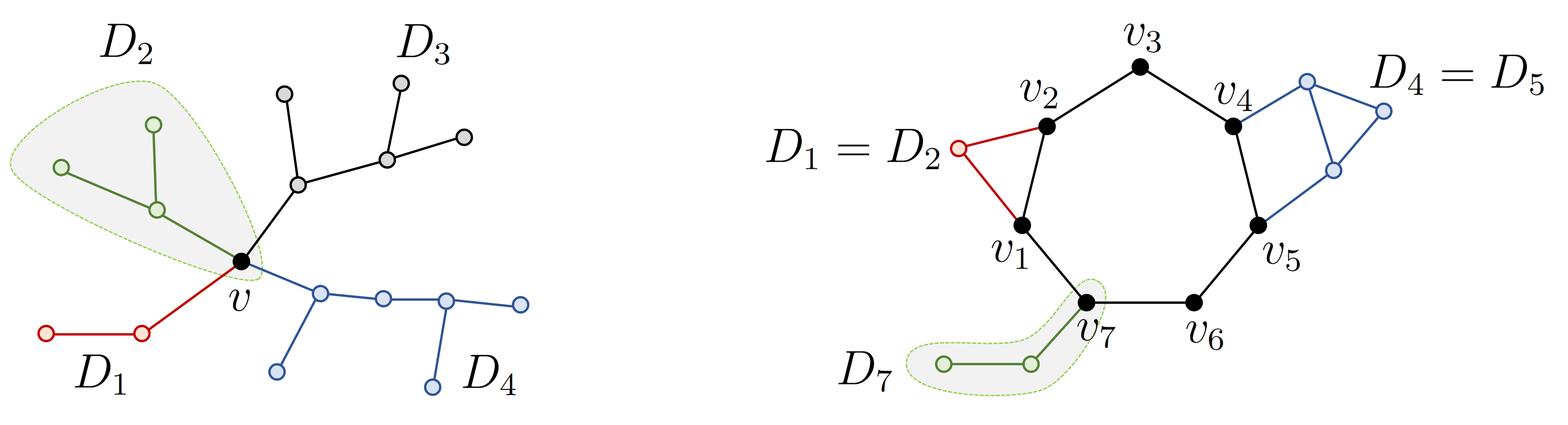
Figure 4.1. The left and right figures illustrate (Case 1) and (Case 2) in the proof of Lemma 4.2, respectively. Note that we have $D_{3}=D_{6}=\emptyset$ at the right figure.

(Case 1: $G$ does not have a cycle, i.e., $G$ is a tree) If every vertex of $G$ has degree at most $2$, then $G$ is a line graph, and thus we can easily divide $E$ into two connected subsets $E^{\prime}$ and $E\setminus E^{\prime}$ satisfying (4.1).

Next, we suppose that a vertex $v\in V$ has degree at least $3$. Since $G$ is a tree, we can decompose $E$ into connected $D_{1},\,D_{2},\,\dots,\,D_{m}$ with $m=\deg(v)\geq 3$, such that the edges in $D_{i}$ and $D_{j}$ ($i\neq j)$ possibly intersect only at $v$ (cf. Figure 4.1-(left)). We impose the condition $|D_{1}|\leq\cdots\leq|D_{m}|$ for convenience.

If $|D_{k}|\geq 3$ for $k=1$ or $2$, it suffices to take $E^{\prime}=D_{k}$. If $|D_{1}|,\,|D_{2}|\leq 2$ but $|D_{1}|+|D_{2}|\geq 3$, we take $E^{\prime}=D_{1}\cup D_{2}$. Finally, if $|D_{1}|=|D_{2}|=1$, we take

$$E^{\prime}=\begin{cases}D_{1}\cup D_{2}\cup\{\text{the edge in }D_{3}\text{ having }v\text{ as an end point}\}&\text{if }m=3\;,\\ D_{1}\cup D_{2}\cup D_{3}&\text{if }m\geq 4\;.\end{cases}$$

(Case 2: $G$ has a cycle) Suppose that $(v_{1},\,v_{2},\,\dots,\,v_{n})$ is a cycle in $G$ in the sense that $\{v_{i},\,v_{i+1}\}\in E$ for all $i\in\llbracket 1,\,n\rrbracket$ with the convention $v_{n+1}=v_{1}$. We denote by $E_{0}$ the edges belonging to this cycle, i.e.,

$$E_{0}=\big{\{}\,\{v_{i},\,v_{i+1}\}:i\in\llbracket 1,\,n\rrbracket\,\big{\}}\;.$$

If $E=E_{0}$, i.e., $G$ is a ring graph, we can easily divide $E$ into two connected subsets $E^{\prime}$ and $E\setminus E^{\prime}$ satisfying (4.1) and hence suppose that $E\setminus E_{0}\neq\emptyset$. For each $i\in\llbracket 1,\,n\rrbracket$, we denote by $D_{i}$ the connected component of $E\setminus E_{0}$ containing the vertex $v_{i}$ so that we have as in Figure 4.1-(right) so that

$$E=E_{0}\cup\Big{(}\,\bigcup_{i=1}^{n}D_{i}\,\Big{)}\;.$$

Note that we may have $D_{i}=D_{j}$ for some $i\neq j$. Since we assumed $E\setminus E_{0}\neq\emptyset$, we can assume without loss of generality that $D_{1}\neq\emptyset$. If $|D_{1}|\geq 3$, we take $E^{\prime}=D_{1}$. Otherwise, we take $E^{\prime}=D_{1}\cup\{\{v_{1},\,v_{2}\},\,\{v_{1},\,v_{n}\}\}$.

This completes the proof of (4.1) and we are done. ∎

Remark 4.3.

We remark that the set $\{3,\,4,\,5,\,6\}$ appeared in the previous lemma cannot be replaced with $\{3,\,4,\,5\}$. For example, in (Case 1) of the proof (cf. Figure 4.1-(left)), the graph with $m=3$ and $|E_{1}|=|E_{2}|=|E_{3}|=2$ provides such a counterexample.

4.2. Counting of configurations with fixed energy

The crucial lemma in the analysis of the Gibbs measure is the following upper and lower bounds for the number of configurations belonging to the set $\mathcal{X}_{i}$, which denotes the collection of configurations with energy $i$ (cf. (3.4)).

Lemma 4.4.

There exists $\theta>1$ such that the following estimates hold.

1. (Upper bound) For all $i\in\mathbb{N}$, we have

   $$|\mathcal{X}_{i}|\leq q^{i+1}\times\sum_{\begin{subarray}{c}n_{3},\,n_{4},\,n_{5},\,n_{6}\geq 0:\\ 3n_{3}+4n_{4}+5n_{5}+6n_{6}=i\end{subarray}}{\theta L^{2}\choose n_{3}}{\theta L^{2}\choose n_{4}}{\theta L^{2}\choose n_{5}}{\theta L^{2}\choose n_{6}}\;.$$

2. (Lower bound) For all $1\leq j<\lfloor\frac{L^{2}}{2}\rfloor$, we have

   $$|\mathcal{X}_{3j}|\geq 4^{j}{\lfloor\frac{L^{2}}{2}\rfloor\choose j}\;.$$

Proof.

(1) As the assertion is obvious for $i=0$ where $|\mathcal{X}_{0}|=q$, we assume $i\neq 0$ so that $i\geq 3$ (since $\mathcal{X}_{1}$ and $\mathcal{X}_{2}$ are empty). Denote by $E(\Lambda^{*})$ the collection of edges of the dual lattice $\Lambda^{*}$ and let $\mathcal{E}_{i}$ be the collection of $E_{0}\subseteq E(\Lambda^{*})$ such that $|E_{0}|=i$. Then, by the arguments given in Section 2.2, we can regard $\mathfrak{A}^{*}(\cdot)$ defined in (2.5) as a map from $\mathcal{X}_{i}$ to $\mathcal{E}_{i}$.

For $\sigma\in\mathcal{X}$, it is immediate that the graph $G[\mathfrak{A}^{*}(\sigma)]$ (cf. Notation 4.1) has no vertex of degree $1$, since if there exists such a vertex, then there is no possible coloring on the six faces of $\Lambda^{*}$ surrounding the vertex which realizes $\mathfrak{A}^{*}(\sigma)$. Therefore, each vertex of $G[\mathfrak{A}^{*}(\sigma)]$ has degree at least two. This implies that each connected component of $G[\mathfrak{A}^{*}(\sigma)]$ has a cycle and hence has at least three edges. Thus, by Lemma 4.2, we can decompose an element of $\mathfrak{A}^{*}(\mathcal{X}_{i})$ by connected components of sizes $3$, $4$, $5$, or $6$. Note that there exists a fixed integer $\theta>1$ such that there are at most $\theta L^{2}$ connected subgraphs of $\Lambda^{*}$ with at most $6$ edges (for all $L$). Combining the observations above concludes that

$$|\mathfrak{A}^{*}(\mathcal{X}_{i})|\leq\sum_{\begin{subarray}{c}n_{3},\,n_{4},\,n_{5},\,n_{6}\geq 0:\\ 3n_{3}+4n_{4}+5n_{5}+6n_{6}=i\end{subarray}}{\theta L^{2}\choose n_{3}}{\theta L^{2}\choose n_{4}}{\theta L^{2}\choose n_{5}}{\theta L^{2}\choose n_{6}}\;.$$ (4.2)

Next, we will show that

$$|(\mathfrak{A}^{*})^{-1}(\eta)|\leq q^{i+1}\;\;\;\;\text{for all }\eta\in\mathfrak{A}^{*}(\mathcal{X}_{i})\;.$$ (4.3)

Indeed, since $\eta\in\mathfrak{A}^{*}(\mathcal{X}_{i})$ has $i$ edges, it divides (the faces of) $\Lambda^{*}$ into at most $i+1$ connected components, where each component must be a monochromatic cluster in each $\sigma\in(\mathfrak{A}^{*})^{-1}(\eta)$. Therefore, there are at most $q^{i+1}$ (indeed, $q\times(q-1)^{i}$) ways to paint these monochromatic clusters and we get (4.3). Part (1) follows directly from (4.2) and (4.3).

(2) If we take an independent set $A$ of size $j$ from $\Lambda$ (i.e., we take $j$ mutually disconnected triangle faces in $\Lambda^{*}$), and assign spins $1$ and $2$ on $A$ and $\Lambda\setminus A$, respectively, then the energy of the corresponding configuration is $3j$ by (2.7). If we select such $j$ vertices one by one, then each selection of a vertex reduces at most four possibilities of the next choice (namely, the selected one and the three adjacent vertices). Since the selection does not depend on the order, there are at least

$$\frac{2L^{2}(2L^{2}-4)\cdots(2L^{2}-4j+4)}{j!}\geq 4^{j}{\lfloor\frac{L^{2}}{2}\rfloor\choose j}$$

ways of selecting such an independent set of size $j$. This concludes the proof of part (2). ∎

4.3. Lemma on concentration

In this subsection, we establish a counting lemma which is useful in the proof of Theorems 3.2 and 3.3. Remark that we regard $\beta=\beta_{L}$ to be dependent of $L$.

Lemma 4.5.

Suppose that $e^{\beta}\ll L^{2/3}$ and moreover two sequences $(g_{1}(L))_{L\in\mathbb{N}}$ and $(g_{2}(L))_{L\in\mathbb{N}}$ satisfy

$$1\ll g_{1}(L)\ll L^{2}e^{-3\beta}\ll g_{2}(L)\;.$$

Then, we have

$$\mu_{\beta}\big{(}\,\mathcal{X}_{[g_{1}(L),\,g_{2}(L)]}\,\big{)}=1-o_{L}(1)\;.$$

Proof.

It is enough to show that

$$\mu_{\beta}\Big{(}\,\bigcup_{i<g_{1}(L)}\mathcal{X}_{i}\,\Big{)}=o_{L}(1)\;\;\;\;\text{and}\;\;\;\;\mu_{\beta}\Big{(}\,\bigcup_{i>g_{2}(L)}\mathcal{X}_{i}\,\Big{)}=o_{L}(1)\;.$$ (4.4)

To prove the first one, it suffices to prove that

$$\sum_{i<g_{1}(L)}|\mathcal{X}_{i}|e^{-\beta i}\ll\sum_{i\geq g_{1}(L)}|\mathcal{X}_{i}|e^{-\beta i}\;.$$ (4.5)

By part (1) of Lemma 4.4, we have

$$\sum_{i<g_{1}(L)}|\mathcal{X}_{i}|e^{-\beta i}\leq q\times\sum_{\begin{subarray}{c}n_{3},\,n_{4},\,n_{5},\,n_{6}\geq 0:\\ 3n_{3}+4n_{4}+5n_{5}+6n_{6}<g_{1}(L)\end{subarray}}{\theta L^{2}\choose n_{3}}{\theta L^{2}\choose n_{4}}{\theta L^{2}\choose n_{5}}{\theta L^{2}\choose n_{6}}(qe^{-\beta})^{3n_{3}+4n_{4}+5n_{5}+6n_{6}}\;.$$

Let $L$ be large enough so that $qe^{-\beta}<1$. Then, the summation at the right-hand side is bounded from above by

$$\sum_{\begin{subarray}{c}n_{3},\,n_{4},\,n_{5},\,n_{6}\geq 0:\\ 3n_{3}+3n_{4}+3n_{5}+3n_{6}<g_{1}(L)\end{subarray}}{\theta L^{2}\choose n_{3}}{\theta L^{2}\choose n_{4}}{\theta L^{2}\choose n_{5}}{\theta L^{2}\choose n_{6}}(qe^{-\beta})^{3n_{3}+3n_{4}+3n_{5}+3n_{6}}$$

$$=\sum_{i<\frac{g_{1}(L)}{3}}\sum_{\begin{subarray}{c}n_{3},\,n_{4},\,n_{5},\,n_{6}\geq 0:\\ n_{3}+n_{4}+n_{5}+n_{6}=i\end{subarray}}{\theta L^{2}\choose n_{3}}{\theta L^{2}\choose n_{4}}{\theta L^{2}\choose n_{5}}{\theta L^{2}\choose n_{6}}(qe^{-\beta})^{3i}=\sum_{i<\frac{g_{1}(L)}{3}}{4\theta L^{2}\choose i}(qe^{-\beta})^{3i}\;,$$ (4.6)

where at the last equality we used a combinatorial identity of the form

$$\sum_{x+y+z+w=k}{a\choose x}{b\choose y}{c\choose z}{d\choose w}={a+b+c+d\choose k}\;.$$ (4.7)

We can further bound the last summation in (4.6) from above by

$$\sum_{i<\frac{g_{1}(L)}{3}}\frac{(4\theta L^{2})^{i}}{i!}(qe^{-\beta})^{3i}\leq\frac{g_{1}(L)+3}{3}\cdot\frac{(4\theta L^{2})^{\frac{g_{1}(L)}{3}}\cdot(qe^{-\beta})^{g_{1}(L)}}{\lfloor\frac{g_{1}(L)}{3}\rfloor!}\leq g_{1}(L)\cdot\Big{(}\frac{CL^{2}e^{-3\beta}}{g_{1}(L)}\Big{)}^{\frac{g_{1}(L)}{3}}$$

using $g_{1}(L)\ll L^{2}e^{-3\beta}$ and an elementary bound $n!\geq n^{n}/e^{n}$. Summing up, we get

$$\sum_{i<g_{1}(L)}|\mathcal{X}_{i}|e^{-\beta i}\leq qg_{1}(L)\cdot\Big{(}\frac{CL^{2}e^{-3\beta}}{g_{1}(L)}\Big{)}^{\frac{g_{1}(L)}{3}}\;.$$ (4.8)

Next, let $\widetilde{g}_{1}(L)=\lfloor g_{1}(L)^{2/3}(L^{2}e^{-3\beta})^{1/3}\rfloor$ so that we have $g_{1}(L)\ll\widetilde{g}_{1}(L)\ll L^{2}e^{-3\beta}$. Then, by part (2) of Lemma 4.4, we have

$$\sum_{i\geq g_{1}(L)}|\mathcal{X}_{i}|e^{-\beta i}\geq|\mathcal{X}_{3\widetilde{g}_{1}(L)}|e^{-3\beta\widetilde{g}_{1}(L)}\geq 4^{\widetilde{g}_{1}(L)}{\lfloor\frac{L^{2}}{2}\rfloor\choose\widetilde{g}_{1}(L)}\times e^{-3\beta\widetilde{g}_{1}(L)}\;.$$

By Stirling’s formula and $\widetilde{g}_{1}(L)\ll L^{2}e^{-3\beta}\ll L^{2}$, this is bounded from below by, for all large enough $L$,

$$\frac{1}{2}(4e)^{\widetilde{g}_{1}(L)}\frac{(\frac{L^{2}}{3})^{\widetilde{g}_{1}(L)}}{\widetilde{g}_{1}(L)^{\widetilde{g}_{1}(L)}\sqrt{2\pi\widetilde{g}_{1}(L)}}\cdot e^{-3\beta\widetilde{g}_{1}(L)}\geq\Big{(}\frac{L^{2}e^{-3\beta}}{\widetilde{g}_{1}(L)}\Big{)}^{\widetilde{g}_{1}(L)}\gg\Big{(}\frac{L^{2}e^{-3\beta}}{\widetilde{g}_{1}(L)}\Big{)}^{g_{1}(L)}\;.$$ (4.9)

Therefore by (4.8) and (4.9), we can reduce the proof of (4.5) into

$$\frac{L^{2}e^{-3\beta}}{\widetilde{g}_{1}(L)}\gg\Big{(}\frac{L^{2}e^{-3\beta}}{g_{1}(L)}\Big{)}^{1/3}\;.$$

This follows from the definition of $\widetilde{g}_{1}(L)$ and the fact that $g_{1}(L)\ll L^{2}e^{-3\beta}$. This proves the first statement in (4.4).

Next, to prove the second estimate of (4.4), it suffices to prove

$$\sum_{i>g_{2}(L)}|\mathcal{X}_{i}|e^{-\beta i}\ll 1$$

since the partition function $Z_{\beta}$ has a trivial lower bound $Z_{\beta}\geq q$ (by only considering the ground states). By a similar computation leading to (4.8), we get

$$\sum_{i>g_{2}(L)}|\mathcal{X}_{i}|e^{-\beta i}\leq q\sum_{i>\frac{g_{2}(L)}{6}}\frac{(4\theta L^{2})^{i}}{i!}(qe^{-\beta})^{3i}\;.$$ (4.10)

Here, Taylor’s theorem on the function $x\mapsto e^{x}$ implies that for $x>0$ and $M\in\mathbb{N}$,

$$\sum_{i>M}\frac{x^{i}}{i!}\leq\max_{t\in[0,\,x]}|e^{t}|\times\frac{x^{M+1}}{(M+1)!}=\frac{e^{x}x^{M+1}}{(M+1)!}\;.$$ (4.11)

Therefore, the right-hand side of (4.10) is bounded from above by

$$e^{CL^{2}e^{-3\beta}}\times\frac{(CL^{2}e^{-3\beta})^{\frac{g_{2}(L)}{6}}}{(\frac{g_{2}(L)}{6})^{\frac{g_{2}(L)}{6}}} \leq\Big{[}\,6C(e^{6C})^{\frac{L^{2}e^{-3\beta}}{g_{2}(L)}}\times\frac{L^{2}e^{-3\beta}}{g_{2}(L)}\,\Big{]}^{\frac{g_{2}(L)}{6}}\;.$$

As $L^{2}e^{-3\beta}\ll g_{2}(L)$, this expression vanishes as $L\rightarrow\infty$. This concludes the proof. ∎

4.4. Proof of Theorems 3.2 and 3.3

Now, we are ready to prove Theorems 3.2 and 3.3. Remark that the constant $\gamma_{0}$ is $\frac{2}{3}$ since we consider the hexagonal lattice.

Proof of Theorem 3.2.

(1) It suffices to prove that, for some constant $C>0$,

$$\sum_{\sigma\in\mathcal{X}\setminus\mathcal{S}}e^{-\beta H(\sigma)}=\sum_{i=3}^{3L^{2}}|\mathcal{X}_{i}|e^{-\beta i}\ll 1\;,$$ (4.12)

where the identity follows from the observation that the minimum non-zero value of the Hamiltonian is $3$ and the maximum is $3L^{2}$. By part (1) of Lemma 4.4, we have (for $qe^{-\beta}<1$)

$$\sum_{i=3}^{3L^{2}}|\mathcal{X}_{i}|e^{-\beta i} \leq q\times\sum_{i=3}^{3L^{2}}\sum_{\begin{subarray}{c}n_{3},\,n_{4},\,n_{5},\,n_{6}\geq 0:\\ 3n_{3}+4n_{4}+5n_{5}+6n_{6}=i\end{subarray}}{\theta L^{2}\choose n_{3}}{\theta L^{2}\choose n_{4}}{\theta L^{2}\choose n_{5}}{\theta L^{2}\choose n_{6}}(qe^{-\beta})^{3n_{3}+4n_{4}+5n_{5}+6n_{6}}$$

$$\leq q\times\sum_{\begin{subarray}{c}n_{3},\,n_{4},\,n_{5},\,n_{6}\geq 0:\\ n_{3}+n_{4}+n_{5}+n_{6}\geq 1\end{subarray}}{\theta L^{2}\choose n_{3}}{\theta L^{2}\choose n_{4}}{\theta L^{2}\choose n_{5}}{\theta L^{2}\choose n_{6}}(qe^{-\beta})^{3n_{3}+3n_{4}+3n_{5}+3n_{6}}\;.$$

Summing up and applying (4.7), we get

$$\sum_{\sigma\in\mathcal{X}\setminus\mathcal{S}}e^{-\beta H(\sigma)}\leq q\sum_{i=1}^{\infty}{4\theta L^{2}\choose i}(qe^{-\beta})^{3i}\leq q\sum_{i=1}^{\infty}\frac{(4\theta q^{3}L^{2}e^{-3\beta})^{i}}{i!}\;.$$

Again applying Taylor’s theorem on the function $x\mapsto e^{x}$ (cf. (4.11)) for $x=4\theta q^{3}L^{2}e^{-3\beta}$, the last summation is bounded by

$$e^{4\theta q^{3}L^{2}e^{-3\beta}}\times(4\theta q^{3}L^{2}e^{-3\beta})\;.$$

This completes the proof of (4.12) since we have $L^{2}e^{-3\beta}\ll 1$ by assumption.

(2) We have $e^{\beta}\ll L^{2/3}$ and therefore as in Lemma 4.5 we can take two sequences $(g_{1}(L))_{L\in\mathbb{N}}$ and $(g_{2}(L))_{L\in\mathbb{N}}$ satisfying

$$1\ll g_{1}(L)\ll L^{2}e^{-3\beta}\ll g_{2}(L)\;.$$

Then, by Lemma 4.5, the measure $\mu_{\beta}$ is concentrated on $\mathcal{X}_{[g_{1}(L),\,g_{2}(L)]}$ and therefore $\mu_{\beta}(\mathcal{S})=o_{L}(1)$. ∎

Proof of Theorem 3.3.

(1) Since $L^{\frac{2}{3}(1-\alpha)}\ll e^{\beta}$, we have $L^{2}e^{-3\beta}\ll cL^{2\alpha}$ for any $c>0$. Thus, we can complete the proof by recalling Lemma 4.5 with any $g_{1}(L)$ such that $1\ll g_{1}(L)\ll L^{2}e^{-3\beta}$ (which is possible since we assumed that $e^{\beta}\ll L^{\gamma_{0}}$) and $g_{2}(L)=cL^{2\alpha}$.

(2) We can take $g_{1}(L)=cL^{2\alpha}$ (and any $g_{2}(L)$ such that $L^{2}e^{-3\beta}\ll g_{2}(L)$) to get $\mu_{\beta}(\mathcal{X}_{[cL^{2\alpha},\,g_{2}(L)]})=1-o_{L}(1)$. This completes the proof. ∎

4.5. Remarks on square lattice case

For the square lattice case, a slightly different version of Lemma 4.2 is required. More precisely, we need a version which is obtained from Lemma 4.2 by replacing the set $\{3,\,4,\,5,\,6\}$ with $\{4,\,5,\,\dots,\,9\}$. This modification comes from the fact that the minimal cycle in the dual graph $\Lambda^{*}$ has three edges in the hexagonal lattice but has four edges in the square lattice case (cf. proof of Lemma 4.4). The proof of this lemma is similar to that of Lemma 4.2 and we will not repeat the proof. As a consequence of this modification, the upper and lower bounds appeared in Lemma 4.4 should be replaced with

$$|\mathcal{X}_{i}|\leq q^{i+1}\times\sum_{\begin{subarray}{c}n_{4},\,n_{5},\,\dots,\,n_{9}\geq 0:\\ 4n_{4}+5n_{5}+\cdots+9n_{9}=i\end{subarray}}{\theta L^{2}\choose n_{4}}{\theta L^{2}\choose n_{5}}\cdots{\theta L^{2}\choose n_{9}}$$

and $|\mathcal{X}_{4j}|\geq 5^{j}{\lfloor\frac{L^{2}}{5}\rfloor\choose j}$ for $1\leq j<\lfloor\frac{L^{2}}{5}\rfloor$, respectively. The constant $\gamma_{0}$ for the square lattice is different to that for the hexagonal one because of this modification.

5. Preliminaries for Energy Landscape

In this section, we introduce several preliminary notation and results which are useful in the subsequent analysis of the energy landscape.

5.1. Strip, bridge and cross.

In this subsection, we provide some crucial notation regarding the structure of the dual lattice $\Lambda^{*}$. We refer to Figure 5.1 for illustrations of the notation defined below and we consistently refer to this figure.

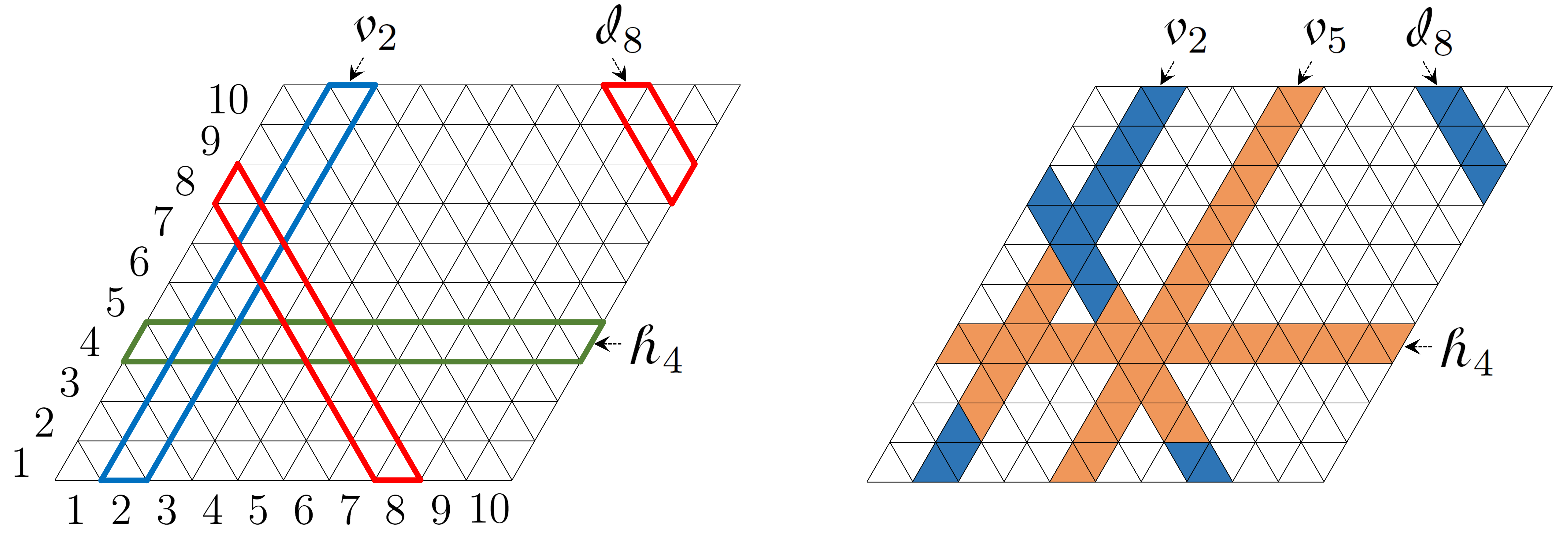
Figure 5.1. (Left) Strips $\scal{h}_{4}$, $\scal{v}_{2}$, and $\scal{d}_{8}$. (Right) Here and in the following figures, white, orange, and blue colors represent spins $a,\,b,\,c$, respectively. Strips $\scal{h}_{4}$ and $\scal{v}_{5}$ are $b$-bridges and thus they form a $b$-cross. Strips $\scal{v}_{2}$ and $\scal{d}_{8}$ are $\{b,\,c\}$-semibridges.

Definition 5.1 (Strip, bridge, cross and semibridge).

We define the crucial concepts here.

1. We denote by a strip the $2L$ consecutive triangles in $\Lambda^{*}$ as illustrated in Figure 5.1-(left). We may regard each strip as a discrete torus $\mathbb{T}_{2L}$ via the obvious manner.

2. There are three possible directions for strips. We call these three directions as horizontal, vertical, and diagonal, and these are highlighted by black, blue, and red lines in Figure 5.1-(left), respectively. For each $\ell\in\mathbb{T}_{L}=\{1,\,2,\,\dots,\,L\}$, the $\ell$-th strip of horizontal, vertical, and diagonal directions are denoted by $\scal{h}_{\ell}$, $\scal{v}_{\ell}$, and $\scal{d}_{\ell}$, respectively, as in Figure 5.1-(left).

3. A strip $\scal{s}$ is called a bridge of $\sigma\in\mathcal{X}$ if all the spins of $\sigma$ in $\scal{s}$ are the same. If this spin is $a$, we call $\scal{s}$ an $a$-bridge of $\sigma$. Furthermore, we can specify the direction of a bridge by calling it a horizontal, vertical, or diagonal bridge of $\sigma$. Finally, the union of two bridges of different directions (of spin $a$) is called a cross (an $a$-cross). We refer to Figure 5.1-(right).

4. A strip $\scal{s}$ is called a semibridge of $\sigma\in\mathcal{X}$, if the strip $\scal{s}$ in $\sigma$ consists of exactly two spins, and moreover the sites in $\scal{s}$ with either of these spins are consecutive. If a semibridge consists of two spins $a$ and $b$, we say that it is an $\{a,\,b\}$-semibridge. We refer to Figure 5.1-(right).

5.2. Low-dimensional decomposition of energy

For each strip $\scal{s}$, the energy of a configuration $\sigma$ on the strip $\scal{s}$ is defined as

$$\Delta H_{\scal{s}}(\sigma)=\sum_{x,\,y\in\scal{s}:\,x\sim y}\mathbf{1}\{\sigma(x)\neq\sigma(y)\}$$

so that by the definition of the Hamiltonian $H$, we have the following decomposition

$$H(\sigma)=\frac{1}{2}\sum_{\ell\in\mathbb{T}_{L}}\big{[}\,\Delta H_{\scal{h}_{\ell}}(\sigma)+\Delta H_{\scal{v}_{\ell}}(\sigma)+\Delta H_{\scal{d}_{\ell}}(\sigma)\,\big{]}\;,$$ (5.1)

where the term $1/2$ appears since each edge is counted twice. The following simple fact is worth mentioning explicitly.

Lemma 5.2.

Suppose that a strip $\scal{s}$ is not a bridge of $\sigma$. Then, we have

$$\Delta H_{\scal{s}}(\sigma)\geq 2\;,$$

and furthermore $\Delta H_{\scal{s}}(\sigma)=2$ if and only if $\scal{s}$ is a semibridge of $\sigma$.

Proof.

The proof is straightforward by identifying a strip $\scal{s}$ with $\mathbb{T}_{2L}$ as in Definition 5.1-(1). ∎

The next lemma provides an elementary lower bound on the number of bridges based on the energy of configurations. Let us denote by $B_{a}(\sigma)$ the number of $a$-bridges in $\sigma\in\mathcal{X}$.

Lemma 5.3.

For $\sigma\in\mathcal{X}$, there are at least $3L-H(\sigma)$ bridges. Moreover, if $\sigma$ has exactly $3L-H(\sigma)$ bridges then all strips are either bridges or semibridges.

Proof.

By (5.1) and Lemma 5.2, we have

$$H(\sigma)\geq\frac{1}{2}\times 2\times\Big{[}\,3L-\sum_{a\in\Omega}B_{a}(\sigma)\,\Big{]}=3L-\sum_{a\in\Omega}B_{a}(\sigma)\;.$$ (5.2)

This proves that there are at least $3L-H(\sigma)$ bridges. Moreover, by Lemma 5.2, a strip which is not a bridge should be a semibridge in order to have the equality in the bound (5.2). This completes the proof. ∎

5.3. Neighborhoods

Recall the notion of paths from (3.1). We say that a path $(\omega_{n})_{n=0}^{N}$ is in $\mathcal{A}\subseteq\mathcal{X}$ if $\omega_{n}\in\mathcal{A}$ for all $n\in\llbracket 0,\,N\rrbracket$. For $t\in\mathbb{R}$, we say that a path $(\omega_{n})_{n=0}^{N}$ is a $t$-path if $H(\omega_{n})\leq t$ for all $n\in\llbracket 0,\,N\rrbracket$.

Definition 5.4.

We define two types of neighborhoods.

1. For $\sigma\in\mathcal{X}$, the neighborhoods $\mathcal{N}(\sigma)$ and $\widehat{\mathcal{N}}(\sigma)$ are defined as

   $$\mathcal{N}(\sigma) =\{\zeta\in\mathcal{X}:\exists\text{a }(2L+1)\text{-path connecting }\sigma\text{ and }\zeta\}\;,$$

   $$\widehat{\mathcal{N}}(\sigma) =\{\zeta\in\mathcal{X}:\exists\text{a }(2L+2)\text{-path connecting }\sigma\text{ and }\zeta\}\;.$$

   Then for $\mathcal{A}\subseteq\mathcal{X}$, we define

   $$\mathcal{N}(\mathcal{A})=\bigcup_{\sigma\in\mathcal{A}}\mathcal{N}(\sigma)\;\;\;\;\text{and}\;\;\;\;\widehat{\mathcal{N}}(\mathcal{A})=\bigcup_{\sigma\in\mathcal{A}}\mathcal{\widehat{N}}(\sigma)\;.$$

   We sometimes refer these as $\mathcal{N}$- and $\widehat{\mathcal{N}}$-neighborhoods, respectively.

2. Let $\mathcal{B}\subseteq\mathcal{X}$. For $\sigma\in\mathcal{X}\setminus\mathcal{B}$, we define

   $$\widehat{\mathcal{N}}(\sigma;\,\mathcal{B})=\{\zeta\in\mathcal{X}:\exists\text{a }(2L+2)\text{-path in }\mathcal{X}\setminus\mathcal{B}\text{ connecting }\sigma\text{ and }\zeta\}\;.$$

   Then for $\mathcal{A}\subseteq\mathcal{X}$ disjoint with $\mathcal{B}$, we define

   $$\widehat{\mathcal{N}}(\mathcal{A};\,\mathcal{B})=\bigcup_{\sigma\in\mathcal{A}}\widehat{\mathcal{N}}(\sigma;\,\mathcal{B})\;.$$

We remark that the numbers $2L+1$ and $2L+2$ appear in the definition since it will be shown that $2L+2$ is the energy barrier $\Gamma$.

6. Energy Barrier

This section provides the first level of investigation of the energy landscape which suffices to prove Theorem 3.1, that is, the energy barrier between ground states is $2L+2$. A deeper analysis of the energy landscape required to prove the Eyring–Kramers formula will be carried out in Section 7.

We collect here notation heavily used in the remainder of the article.

Notation 6.1.

Here, the alphabets $\scal{h},\,\scal{v},\,\scal{d}$ stand for horizontal, vertical, and diagonal, respectively.

1. We say that $(A,\,B)$ is a proper partition (of $\Omega$) if $A,\,B\neq\emptyset$, $A\cup B=\Omega$, and $A\cap B=\emptyset$.

2. Let $L\geq 2$ and denote by $\mathfrak{S}_{L}$ the collection of connected subsets of $\mathbb{T}_{L}$. For example, we have $\emptyset,\,\{2\},\,\{2,\,3,\,4,\,5\},\,\{6,\,1,\,2\}\in\mathfrak{S}_{6}$ (since $6$ and $1$ are neighboring in $\mathbb{T}_{6}$).

   1. For $P,\,P^{\prime}\in\mathfrak{S}_{L}$, we write $P\prec P^{\prime}$ if $P\subseteq P^{\prime}$ and $|P^{\prime}|=|P|+1$.

   2. For each $P\in\mathfrak{S}_{L}$, we write

      $$\scal{h}(P)=\bigcup_{\ell\in P}\scal{h}_{\ell}\;,\;\;\;\;\scal{v}(P)=\bigcup_{\ell\in P}\scal{v}_{\ell}\;,\;\;\;\;\text{and}\;\;\;\;\scal{d}(P)=\bigcup_{\ell\in P}\scal{d}_{\ell}\;.$$

3. We regard the dual lattice $\Lambda^{*}$ as the collection of triangles (corresponding to the sites, or vertices of $\Lambda$) and hence we say that $U$ is a subset of $\Lambda^{*}$ (i.e., $U\subseteq\Lambda^{*}$) if $U$ is a collection of triangles in $\Lambda^{*}$. For example, a strip is a subset of $\Lambda^{*}$ consisting of $2L$ triangles.

4. For each $U\subseteq\Lambda^{*}$ and $a,\,b\in\Omega$, we write $\xi_{U}^{a,\,b}\in\mathcal{X}$ the configuration whose spins are $b$ on the sites corresponding to the triangles in $U$ and $a$ on the remainder.

6.1. Canonical configurations

In this subsection, we define the canonical configurations between ground states. These canonical configurations provide the backbone of the saddle structure. We shall see in the sequel that the saddle structure is completed by attaching dead-end structures or bypasses at this backbone. We define canonical configurations in several steps. The first step is devoted to define the regular configurations which are indeed special forms of canonical configurations.

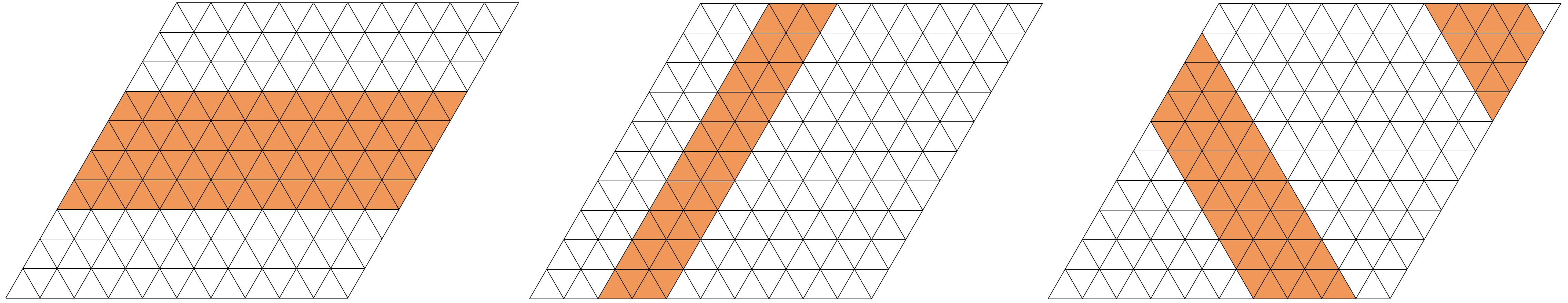
Figure 6.1. Example of regular configurations: $\xi_{\scal{h}(\llbracket 4,\,7\rrbracket)}^{a,\,b}$ (left), $\xi_{\scal{v}(\llbracket 3,\,4\rrbracket)}^{a,\,b}$ (middle), and $\xi_{\scal{d}(\llbracket 7,\,9\rrbracket)}^{a,\,b}$ (right).

Definition 6.2 (Regular configurations).

Fix $a,\,b\in\Omega$. We recall Notation 6.1.

• A configuration of the form $\xi_{\scal{h}(P)}^{a,\,b}$, $\xi_{\scal{v}(P)}^{a,\,b}$, or $\xi_{\scal{d}(P)}^{a,\,b}$ for some $P\in\mathfrak{S}_{L}$ is called a horizontal, vertical, or diagonal regular configuration between $\mathbf{a}$ and $\mathbf{b}$, respectively. We refer to Figure 6.1 for illustrations.

• For $n\in\llbracket 0,\,L\rrbracket$, we define

  $$\mathcal{R}_{n}^{a,\,b}=\bigcup_{P\in\mathfrak{S}_{L}:\,|P|=n}\big{\{}\,\xi_{\scal{h}(P)}^{a,\,b},\,\xi_{\scal{v}(P)}^{a,\,b},\,\xi_{\scal{d}(P)}^{a,\,b}\,\big{\}}\;\;\;\;\text{and}\;\;\;\;\mathcal{R}^{a,\,b}=\bigcup_{n=0}^{L}\mathcal{R}_{n}^{a,\,b}\;.$$

  Then for a proper partition $(A,\,B)$, we write

  $$\mathcal{R}_{n}^{A,\,B}=\bigcup_{a\in A}\bigcup_{b\in B}\mathcal{R}_{n}^{a,\,b}\;\;\;\;\text{and}\;\;\;\;\mathcal{R}^{A,\,B}=\bigcup_{a\in A}\bigcup_{b\in B}\mathcal{R}^{a,\,b}\;.$$

Canonical configurations are now defined as the ones obtained by adding suitable protuberances at a monochromatic cluster of a regular configuration. To carry this out rigorously, we first define canonical sets.

Definition 6.3 (One-dimensional canonical sets).

We say that $U\subseteq\scal{s}$ for some strip $\scal{s}$ is an one-dimensional canonical set if $U\neq\emptyset,\,\scal{s}$ and either $U$ is connected (we remark again that two triangles sharing only a vertex are not connected) as in the two left figures below, or $|U|$ is even and $U$ can be decomposed into two disjoint, connected components $U_{1}$ and $U_{2}$ such that $|U_{2}|=1$ and that $U_{1}$ and $U_{2}$ share a vertex in $\Lambda^{*}$ as in the rightmost figure below.

We now define the general canonical sets.

Figure 6.2. Canonical sets and configurations. For the first three figures, the sets of orange triangles are canonical sets between $\scal{h}(P)$ and $\scal{h}(P^{\prime})$ where $P=\llbracket 1,\,4\rrbracket$ and $P^{\prime}=\llbracket 1,\,5\rrbracket$. If we assign spins $a$ and $b$ at white and orange triangles, respectively, then the configurations corresponding to the first, second, and third figures belong to $\mathcal{C}_{\scal{h}(P,\,P^{\prime}),\,\scal{o}}^{a,\,b}$, $\mathcal{C}_{\scal{h}(P,\,P^{\prime}),\,\scal{e}}^{a,\,b}$, and $\mathcal{C}_{\scal{h}(P,\,P^{\prime}),\,\scal{e}}^{a,\,b}$, respectively. Note that the set of orange triangles at the rightmost figure is not a canonical set since the condition (6.1) is violated.

Definition 6.4 (Canonical sets).

Fix $a,\,b\in\Omega$, $\scal{s}\in\{\scal{h},\,\scal{v},\,\scal{d}\}$, and $P,\,P^{\prime}\in\mathfrak{S}_{L}$ such that $P\prec P^{\prime}$. Let $P^{\prime}\setminus P=\{\ell\}$. We now define the canonical sets between $\scal{s}(P)$ and $\scal{s}(P^{\prime})$. We refer to Figure 6.2.

1. A set $\mathfrak{p}\subseteq\scal{s}_{\ell}$ is called a protuberance attached to $\scal{s}(P)$ if $\mathfrak{p}$ is an one-dimensional canonical set and moreover, for $|P|\in\llbracket 1,\,L-2\rrbracket$, it holds that

   $$\big{|}\,\{x\in\mathfrak{p}:x\text{ shares a side with some }y\in\scal{s}(P)\}\,\big{|}\geq\frac{|\mathfrak{p}|}{2}\;.$$ (6.1)

2. The set $\scal{s}(P)\cup\mathfrak{p}$, where $\mathfrak{p}$ is a protuberance attached to $\scal{s}(P)$, is called a canonical set between $\scal{s}(P)$ and $\scal{s}(P^{\prime})$.

We are now finally able to define the canonical configurations. In the following definition, the alphabets $\scal{o}$ and $\scal{e}$ in the subscripts stand for odd and even, respectively.

Definition 6.5 (Canonical configurations).

We define the canonical configurations (we refer to Figure 6.2 for an illustrations).

1. Fix $a,\,b\in\Omega$, $\scal{s}\in\{\scal{h},\,\scal{v},\,\scal{d}\}$ and $P,\,P^{\prime}\in\mathfrak{S}_{L}$ with $P\prec P^{\prime}$. We say that a configuration $\sigma\in\mathcal{X}$ is a canonical configuration between two regular configurations $\xi_{\scal{s}(P)}^{a,\,b}$ and $\xi_{\scal{s}(P^{\prime})}^{a,\,b}$ if

   $$\sigma=\xi_{A}^{a,\,b}\text{ for some canonical set }A\text{ between }\scal{s}(P)\text{ and }\scal{s}(P^{\prime})\;.$$

   We denote by $\widetilde{\mathcal{C}}_{\scal{s}(P,\,P^{\prime})}^{a,\,b}$ the collection of canonical configurations between $\xi_{\scal{s}(P)}^{a,\,b}$ and $\xi_{\scal{s}(P^{\prime})}^{a,\,b}$.

   1. For each $\sigma=\xi_{A}^{a,\,b}\in\widetilde{\mathcal{C}}_{\scal{s}(P,\,P^{\prime})}^{a,\,b}$, we can decompose $A$ into $\scal{s}(P)$ and the protuberance attached to it (cf. Definition 6.4). We denote this protuberance by $\mathfrak{p}^{a,\,b}(\sigma)$.

   2. We write

      $$\mathcal{C}_{\scal{s}(P,\,P^{\prime})}^{a,\,b} =\widetilde{\mathcal{C}}_{\scal{s}(P,\,P^{\prime})}^{a,\,b}\cup\big{\{}\,\xi_{\scal{s}(P)}^{a,\,b},\,\xi_{\scal{s}(P^{\prime})}^{a,\,b}\,\big{\}}\;,$$

      $$\mathcal{C}_{\scal{s}(P,\,P^{\prime}),\,\scal{o}}^{a,\,b} =\big{\{}\,\sigma\in\widetilde{\mathcal{C}}_{\scal{s}(P,\,P^{\prime})}^{a,\,b}:|\mathfrak{p}^{a,\,b}(\sigma)|\text{ is odd}\,\big{\}}\;,$$

      $$\mathcal{C}_{\scal{s}(P,\,P^{\prime}),\,\scal{e}}^{a,\,b} =\big{\{}\,\sigma\in\widetilde{\mathcal{C}}_{\scal{s}(P,\,P^{\prime})}^{a,\,b}:|\mathfrak{p}^{a,\,b}(\sigma)|\text{ is even}\,\big{\}}\;.$$

2. For $n\in\llbracket 0,\,L-1\rrbracket$ and $a,\,b\in\Omega$, we define

   $$\mathcal{C}_{n}^{a,\,b}=\bigcup_{\scal{s}\in\{\scal{h},\,\scal{v},\,\scal{d}\}}\bigcup_{P\prec P^{\prime}:\,|P|=n}\mathcal{C}_{\scal{s}(P,\,P^{\prime})}^{a,\,b}\;,$$

   and define $\mathcal{C}_{n,\,\scal{o}}^{a,\,b}$ and $\mathcal{C}_{n,\,\scal{e}}^{a,\,b}$ in the same manner. The configurations belonging to $\mathcal{C}_{n}^{a,\,b}$ for some $n\in\llbracket 0,\,L-1\rrbracket$ are called canonical configurations between $\mathbf{a}$ and $\mathbf{b}$.

3. For each proper partition $(A,\,B)$ (cf. Notation 6.1), we write

   $$\mathcal{C}_{n,\,\scal{o}}^{A,\,B}=\bigcup_{a\in A}\bigcup_{b\in B}\mathcal{C}_{n,\,\scal{o}}^{a,\,b}\;\;\;\;\text{and}\;\;\;\;\mathcal{C}_{n,\,\scal{e}}^{A,\,B}=\bigcup_{a\in A}\bigcup_{b\in B}\mathcal{C}_{n,\,\scal{e}}^{a,\,b}\;.$$

Remark 6.6 (Energy of canonical configurations).

The following properties of regular and canonical configurations are straightforward from the definitions. In particular, the discussion on Section 2.2 or (5.1) can be used, and we omit the detail of the proof. Let $a,\,b\in\Omega$.

1. For $n\in\llbracket 1,\,L-2\rrbracket$, we can decompose

   $$\mathcal{C}_{n}^{a,\,b}=\mathcal{R}_{n}^{a,\,b}\cup\mathcal{R}_{n+1}^{a,\,b}\cup\mathcal{C}_{n,\,\scal{o}}^{a,\,b}\cup\mathcal{C}_{n,\,\scal{e}}^{a,\,b}$$

   and we have

   $$H(\sigma)=\begin{cases}2L&\text{if }\sigma\in\mathcal{R}_{n}^{a,\,b}\cup\mathcal{R}_{n+1}^{a,\,b}\;,\\ 2L+1&\text{if }\sigma\in\mathcal{C}_{n,\,\scal{o}}^{a,\,b}\;,\\ 2L+2&\text{if }\sigma\in\mathcal{C}_{n,\,\scal{e}}^{a,\,b}\;.\end{cases}$$

2. If $\sigma\in\mathcal{C}_{n}^{a,\,b}$ for $n=0$ or $L-1$, we have $H(\sigma)\leq 2L+1$.

In conclusion, we have $H(\sigma)\leq 2L+2$ for all canonical configurations $\sigma$.

Remark 6.7 (Canonical paths).

Fix $a,\,b\in\Omega$, $\scal{s}\in\{\scal{h},\,\scal{v},\,\scal{d}\}$, and $P,\,P^{\prime}\in\mathfrak{S}_{L}$ with $P\prec P^{\prime}$. Then, it is clear by definition that there are natural paths in $\mathcal{C}_{\scal{s}(P,\,P^{\prime})}^{a,\,b}$ from $\xi_{\scal{s}(P)}^{a,\,b}$ to $\xi_{\scal{s}(P^{\prime})}^{a,\,b}$ as in the following figure.

Figure 6.3. Canonical path from $\xi_{\scal{h}(\llbracket 4,\,7\rrbracket)}^{a,\,b}$ to $\xi_{\scal{h}(\llbracket 4,\,8\rrbracket)}^{a,\,b}$.

These paths are called canonical paths between $\xi_{\scal{s}(P)}^{a,\,b}$ and $\xi_{\scal{s}(P^{\prime})}^{a,\,b}$. By attaching the canonical paths consecutively, one can obtain a path between $\mathbf{a}$ and $\mathbf{b}$. This path is called a canonical path between $\mathbf{a}$ and $\mathbf{b}$. Note that there are numerous possible canonical paths between $\mathbf{a}$ and $\mathbf{b}$, and that each canonical path is a $(2L+2)$-path (cf. Section 5.3) by Remark 6.6 above.

6.2. Configurations with low energy

Since the energy barrier between ground states is $2L+2$ (as will be proved in this section), the saddle structure between ground states is essentially the $\widehat{\mathcal{N}}$-neighborhood (cf. Definition 5.4) of canonical configurations. Therefore, to understand the saddle structure, it is crucial to characterize the configurations with energy exactly $2L+2$. This characterization is relatively simple for the square lattice (cf. [20, Proposition 6.8 and Lemma 7.2]), as dead-ends are attached only at the very end of the canonical paths. However, this characterization is highly non-trivial for the hexagonal lattice, as we shall see that a complicated dead-end structure is attached at each regular configuration. This and the next subsections are devoted to study this structure.

A configuration $\sigma$ is called cross-free if it does not have a cross (cf. Definition 5.1-(3)). The purpose of the current subsection is to characterize all the cross-free configurations $\sigma$ such that $H(\sigma)\leq 2L+2$. We first prove that a cross-free configuration $\sigma$ has energy at least $2L$, and moreover the energy is exactly $2L$ if and only if $\sigma$ is a regular configuration (cf. Definition 6.2).

Proposition 6.8.

Suppose that a cross-free configuration $\sigma\in\mathcal{X}$ satisfies $H(\sigma)\leq 2L$. Then, $\sigma$ is a regular configuration, i.e., $\sigma\in\mathcal{R}_{n}^{a,\,b}$ for some $a,\,b\in\Omega$ and $n\in\llbracket 1,\,L-1\rrbracket$. In particular, we have $H(\sigma)=2L$.

Proof.

We fix a cross-free configuration $\sigma\in\mathcal{X}$ with $H(\sigma)\leq 2L$. By Lemma 5.3, $\sigma$ has at least $L$ bridges. Since these bridges must be of the same direction, there are exactly $L$ bridges of the same direction (say, horizontal), and by the second assertion of Lemma 5.3, all the vertical and diagonal strips must be semibridges of the same form. We can conclude that $\sigma$ is a regular configuration by combining the observations above. ∎

It now remains to characterize cross-free configurations with energy $2L+1$ or $2L+2$. The following lemma is useful for those characterizations.

Lemma 6.9.

Suppose that a cross-free configuration $\sigma\in\mathcal{X}$ satisfies $H(\sigma)\leq 2L+2$, has $k\in\{L-2,\,L-1\}$ horizontal bridges, and has at least one vertical or diagonal semibridge. Then, the following statements hold for the configuration $\sigma$.

1. There exist two spins $a,\,b\in\Omega$ such that all horizontal bridges are either $a$- or $b$-bridges.

2. Following (1), define two sets $P_{a}$ and $P_{b}$ by

   $$P_{c}=\{\ell\in\mathbb{T}_{L}:\scal{h}_{\ell}\text{ is a }c\text{-bridge}\}\;\;\;\;;\;c\in\{a,\,b\}\;.$$ (6.2)

   Suppose that $P_{a},\,P_{b}\neq\emptyset$. Then, we have $P_{a},\,P_{b}\in\mathfrak{S}_{L}$ and moreover

   1. if $k=L-2$, then all non-bridge strips are $\{a,\,b\}$-semibridges and $H(\sigma)=2L+2$,

   2. if $k=L-1$ and $H(\sigma)\leq 2L+1$, then all non-bridge strips are $\{a,\,b\}$-semibridges.

Remark 6.10.

The conclusion $P_{a},\,P_{b}\in\mathfrak{S}_{L}$ holds even when either $P_{a}$ or $P_{b}$ is empty, but its proof will be given later in Lemma 6.15.

Proof of Lemma 6.9.

(1) The conclusion is immediate since if the vertical or diagonal semibridge of $\sigma$ (which exists because of the assumption of the lemma) is an $\{a,\,b\}$-semibridge for some $a,\,b\in\Omega$, then each horizontal bridge must be either $a$- or $b$-bridge.

(2) Suppose first that no $a$-bridge is adjacent to a $b$-bridge. Then as $P_{a},\,P_{b}\neq\emptyset$ and $k\leq L-1$, we may take one connected subset $C_{a}$ of $P_{a}$ so that $|C_{a}|\leq L-2$. Then, the two strips adjacent to $C_{a}$ must not be $b$-bridges, so that they are not bridges. Then since $k\geq L-2$, we conclude that $C_{a}=P_{a}$ and all the strips which are not adjacent to $C_{a}$ are $b$-bridges. This implies that $P_{a},\,P_{b}\in\mathfrak{S}_{L}$.

Next, suppose that some $a$-bridge is adjacent to a $b$-bridge. Without loss of generality, we assume that $1\in P_{a}$ and $L\in P_{b}$. Let $m=\max\{i\in\llbracket 1,\,L-1\rrbracket:i\in P_{a}\}$ and we claim that $P_{a}=\llbracket 1,\,m\rrbracket$. There is nothing to prove if $m=1$ or $2$, since the claim holds immediately. Suppose $m\geq 3$ and there exists $i\in\llbracket 2,\,m-1\rrbracket$ such that $i\notin P_{a}$. Then, there exists a triangle in the $i$-th horizontal strip at which the spin is not $a$. The vertical and diagonal strips containing this triangle have energy at least $4$, because $1\in P_{a}$, $m\in P_{a}$, and $L\in P_{b}$. All the vertical and diagonal strips other than these two have energy at least $2$ (since the configuration $\sigma$ is cross-free). Since at least one of the horizontal strip must be a non-bridge and has energy at least $2$, we can conclude from (5.1) that

$$H(\sigma)\geq\frac{1}{2}\big{[}\,2+[4+2(L-1)]+[4+2(L-1)]\,\big{]}=2L+3\;.$$

This yield a contradiction and thus we can conclude that $P_{a}=\llbracket 1,\,m\rrbracket\in\mathfrak{S}_{L}$. The proof of $P_{b}\in\mathfrak{S}_{L}$ is the same.

(2-a) For this case, we first note that there are $L-2$ bridges. If $H(\sigma)\leq 2L+1$, by Lemma 5.3, there are at least $3L-H(\sigma)\geq L-1$ bridges and we get a contradiction. Hence, we have $H(\sigma)=2L+2$ and there are $3L-H(\sigma)$ bridges; hence, by the second assertion of Lemma 5.3 all the non-bridge strips are semibridges. It is clear that indeed, they must be $\{a,\,b\}$-semibridges.

(2-b) The proof for this part is almost identical to (2-a) and we omit the detail. ∎

We next characterize all the cross-free configurations with energy $2L+1$. Indeed, they must be canonical configurations.

Proposition 6.11.

Suppose that a cross-free configuration $\sigma\in\mathcal{X}$ satisfies $H(\sigma)=2L+1$. Then, $\sigma\in\mathcal{C}_{n,\,\scal{o}}^{a,\,b}$ for some $a,\,b\in\Omega$ and $n\in\llbracket 0,\,L-1\rrbracket$. Moreover, if $n=0$ (resp. $n=L-1$), then $|\mathfrak{p}^{a,\,b}(\sigma)|=2L-1$ (resp. $|\mathfrak{p}^{a,\,b}(\sigma)|=1$).

Proof.

By Lemma 5.3, the configuration $\sigma$ has at least $L-1$ bridges. Since $\sigma$ is cross-free, these bridges are of the same direction, say horizontal. If there are $L$ horizontal bridges, then all the vertical and diagonal strips are of the same form and thus the energy of $\sigma$ should be a multiple of $L$ in view of (5.1). It contradicts $H(\sigma)=2L+1$, and hence there are exactly $L-1=3L-H(\sigma)$ bridges. By the second assertion of Lemma 5.3, all the non-bridge strips are semibridges. Now, by Lemma 6.9, there exist $a,\,b\in\Omega$ such that all the horizontal bridges are either $a$- or $b$-bridges. Define $P_{a}$ and $P_{b}$ as in Lemma 6.9 and write $\{\ell\}=\mathbb{T}_{L}\setminus(P_{a}\cup P_{b})$.

Suppose first that either $P_{a}$ or $P_{b}$ is empty, say $P_{b}=\emptyset$ and $P_{a}=\mathbb{T}_{L}\setminus\{\ell\}$. Then as all strips are either bridges or semibridges, we conclude that $\scal{h}_{\ell}$ is an $\{a,\,c\}$-semibridge for some $c\neq a$. As $\sigma$ is cross-free, we must have $|\mathfrak{p}^{a,\,c}(\sigma)|=2L-1$. The other case $P_{a}=\emptyset$ can be handled identically.

Next, suppose that $P_{a},\,P_{b}\neq\emptyset$ so that we can apply case (2-b) of Lemma 6.9, which implies that $\scal{h}_{\ell}$ is an $\{a,\,b\}$-semibridge. As illustrated in the figure below, since all the vertical and diagonal strips are semibridge, we can deduce that the set of triangles in $\scal{h}_{\ell}$ with spin $b$ should be an odd protuberance (cf. Definition 6.5) between $\xi_{\scal{h}(P)}^{a,\,b}$ and $\xi_{\scal{h}(P^{\prime})}^{a,\,b}$. Note that for the other cases vertical strip with black bold boundary is not a semibridge.

Therefore, we can conclude that $\sigma\in\mathcal{C}_{n,\,\scal{o}}^{a,\,b}$ for some $n\in\llbracket 1,\,L-2\rrbracket$. ∎

Now, it remains to characterize the cross-free configurations with energy $2L+2$. To this end, we introduce six different types of cross-free configurations with energy $2L+2$ in the following definition.

Definition 6.12 (Cross-free configurations with energy $2L+2$).

The following types characterize the cross-free configurations with energy $2L+2$. We refer to Figure 6.4 below for illustrations and to (5.1) for the verification of the fact that these configurations (except (MB)) have energy $2L+2$.

• One-sided Double Protuberances: two odd protuberances are attached to one side of a regular configuration.

• Two-sided Double Protuberances: two odd protuberances are attached to different sides of a regular configuration.

• Superimposed Protuberances: an odd protuberance is attached to a regular configuration, and another smaller odd protuberance is attached to the first odd protuberance.

• Even Protuberance: an even protuberance is attached to a regular configuration.

• Peculiar Protuberance: a protuberance of a third spin and of size $1$ is attached to a regular configuration.

• Monochromatic Bridges: all the bridges are parallel and of the same spin, where more refined characterization of this type will be given in Lemma 6.15.

Figure 6.4. Six types of cross-free configurations with energy $2L+2$ introduced in Definition 6.12. We refer to Figures 6.5 and 6.6 for more refined characterization of type (MB).

Now, we are finally ready to characterize cross-free configurations with energy $2L+2$.

Proposition 6.13.

Suppose that a cross-free configuration $\sigma\in\mathcal{X}$ satisfies $H(\sigma)=2L+2$. Then, $\sigma$ is of one of the six types introduced in Definition 6.12.

Proof.

By Lemma 5.3, $\sigma$ has at least $L-2$ bridges. Since $\sigma$ is cross-free, these bridges are of the same direction, say horizontal. Then, as in the proof of Proposition 6.11, we can observe that the number of horizontal bridges cannot be $L$ and thus the number of horizontal bridges should be either $L-1$ or $L-2$.

(Case 1: $\sigma$ has $L-1$ horizontal bridges) If there is no vertical or diagonal semibridge, we must have $\Delta H_{\scal{v}_{\ell}}(\sigma),\,\Delta H_{\scal{d}_{\ell}}(\sigma)\geq 3$ for all $\ell\in\mathbb{T}_{L}$ and therefore by (5.1), we get $H(\sigma)\geq 3L$ which yields a contradiction. Hence, there exists at least one vertical or diagonal semibridge and thus by Lemma 6.9, there exist $a,\,b\in\Omega$ such that all the horizontal bridges are $a$- or $b$-bridges. Let us define $P_{a}$ and $P_{b}$ as in Lemma 6.9 and let $\{\ell_{0}\}=\mathbb{T}_{L}\setminus(P_{a}\cup P_{b})$. If $P_{a}=\emptyset$ or $P_{b}=\emptyset$, then $\sigma$ is of type (MB) by definition. Now, we assume that $P_{a},\,P_{b}\neq\emptyset$.

Case 1-1: The strip $\scal{h}_{\ell_{0}}$ contains a triangle with spin which is not $a$ or $b$. If there are two or more such triangles, then there are at least three vertical or diagonal strips containing these triangles with energy at least $3$. Since all the other vertical and diagonal strips have energy at least $2$, we can conclude from (5.1) that

$$H(\sigma)\geq\frac{1}{2}\big{[}\,2+3\times 3+(2L-3)\times 2\,\big{]}>2L+2$$

which yields a contradiction. Therefore, the strip $\scal{h}_{\ell_{0}}$ contains exactly one triangle with spin which is not $a$ or $b$. The vertical and diagonal strips containing this triangle have energy at least $3$. Thus, if the strip $\scal{h}_{\ell_{0}}$ has energy at least $3$, we similarly get a contradiction since we should have

$$H(\sigma)\geq\frac{1}{2}\big{[}\,3+2\times 3+(2L-2)\times 2\,\big{]}>2L+2\;.$$

Therefore, the strip $\scal{h}_{\ell_{0}}$ has energy $2$. This implies that all the triangles in this strip other than the one with spin $c$ have the same spin, which is either $a$ or $b$. Hence, $\sigma$ is of type (PP).

Case 1-2: The strip $\scal{h}_{\ell_{0}}$ consists of spins $a$ and $b$ only. By (5.1), the energy of this strip is at most $4$, and hence is either $2$ or $4$ (since it cannot be an odd integer). If the energy of this strip is $2$, i.e., it is an $\{a,\,b\}$-semibridge by Lemma 5.2, we can check with the argument given in the proof of Proposition 6.11 based on Figure 6.4 that the only possible form of configuration $\sigma$ is of type (EP). On the other hand, if the energy of this strip is $4$, then in view of (5.1), all the vertical and diagonal bridges must have energy $2$ and thus must be semibridges. Since this strip $\scal{h}_{\ell_{0}}$ of energy $4$ is divided into four connected components where two of them are of spin $a$ and the remaining two are of spin $b$, by the same argument given in Proposition 6.11 based on Figure 6.4, we can readily check that $\sigma$ is of type (ODP).

(Case 2: $\sigma$ has $L-2$ horizontal bridges) By the second statement of Lemma 5.3, we can still apply Lemma 6.9, and we can follow the same argument with (Case 1) above to handle the case where $P_{a}$ or $P_{b}$ is empty. Hence, let us suppose that $P_{a},\,P_{b}\neq\emptyset$ and write $\mathbb{T}_{L}\setminus(P_{a}\cup P_{b})=\{\ell_{1},\,\ell_{2}\}$. By (2) of Lemma 6.9, we have $P_{a},\,P_{b}\in\mathfrak{S}_{L}$ and hence we can assume without loss of generality that $P_{a}=\llbracket 1,\,m\rrbracket$ so that

$$\{\ell_{1},\,\ell_{2}\}\in\big{\{}\,\{L,\,m+1\},\,\{m+1,\,m+2\},\,\{L-1,\,L\}\,\big{\}}\;.$$

Note from (2-a) of Lemma 6.9 that

$$\text{all the non-bridge strips of }\sigma\text{ are }\{a,\,b\}\text{-semibridges}.$$ (6.3)

If $\{\ell_{1},\,\ell_{2}\}=\{L,\,m+1\}$, by the same argument with Proposition 6.11, strips $\scal{h}_{\ell_{1}}$ and $\scal{h}_{\ell_{2}}$ should be aligned as in the middle one of Figure 6.4 in order to achieve (6.3), and we can conclude that $\sigma$ is of type (TDP). A similar argument indicates that if $\{\ell_{1},\,\ell_{2}\}=\{m+1,\,m+2\}$ or $\{L-1,\,L\}$, the configuration $\sigma$ should be of type (SP) to fulfill (6.3).

Hence, we demonstrated that for any cases, $\sigma$ is one of the six types given in Definition 6.12. ∎

Remark 6.14.

A careful reading of the proof of the previous proposition reveals that, if $\sigma$ is of type (MB) then it has either $L-1$ or $L-2$ parallel bridges.

In the next lemmas, we investigate more on the configurations of type (MB), since the definition of this type is vague and thus more detailed understanding is crucially required to analyze the energy landscape of $\mathcal{N}$-neighborhoods of the ground states. In the analyses carried out below, we will omit elementary details in the characterization of possible forms, since it always reduces to a small number of subcases that should be tediously checked case by case.

Lemma 6.15.

Suppose that $\sigma\in\mathcal{X}$ is of type (MB) with parallel bridges of spin $a\in\Omega$. Then, exactly one of $(\star)$ and $(\star\star)$ given below holds.

1. There exists a $(2L+2)$-path $(\omega_{n})_{n=0}^{N}$ from $\sigma$ to $\mathbf{a}$ so that $N\leq 4L$ and each configuration $\omega_{n}$ has at least $L-2$ $a$-bridges.

2. The configuration $\sigma$ is isolated in the sense that $\widehat{\mathcal{N}}(\sigma)=\{\sigma\}$.

Proof.

It is immediate that $(\star)$ and $(\star\star)$ cannot hold simultaneously. Hence, it suffices to prove that $\sigma$ satisfies $(\star)$ or $(\star\star)$. Without loss of generality, we assume that the parallel $a$-bridges are horizontal, and define $P_{a}$ as in (6.2) so that we have $|P_{a}|=L-1$ or $L-2$ by Remark 6.14.

(Case 1: $|P_{a}|=L-1$) Without loss of generality, write $\mathbb{T}_{L}\setminus P_{a}=\{1\}$.

If there are two adjacent triangles in $\scal{h}_{1}$ with spin $a$, we can find an $a$-cross and therefore we get a contradiction to the fact that $\sigma$ is cross-free. Hence, the strip $\scal{h}_{1}$ cannot have consecutive triangles with spin $a$. Moreover, since all the vertical and diagonal strips have energy at least $2$, by (5.1), we have $\Delta H_{\scal{h}_{1}}(\sigma)\leq 4$. From this, we can readily deduce that $\sigma$ should be of one of the four types (MB1)-(MB4) as in Figure 6.5.

Figure 6.5. Types (MB1)-(MB4): We can update the triangles according to the indicated arrow starting from the one with red bold boundary to reach $\mathbf{a}$. One can change the starting triangle to the ones with black bold boundary and then modify the order of updates.

We now demonstrate that $(\star)$ holds for all these types. For types (MB1)-(MB3), we select any triangle adjacent to a triangle with spin $a$, and for type (MB4), we select a triangle adjacent to a triangle with different spin. Then, we update the spins in $\scal{h}_{1}$ to $a$ successively from the selected triangle to obtain the configuration $\mathbf{a}$ (cf. Figure 6.5). This procedure provides a $(2L+2)$-path connecting $\sigma$ and $\mathbf{a}$ of length at most $2L$. It is immediate that all the configurations visited by this path have at least $2L-1$ $a$-bridges and hence we can verify the condition $(\star)$ for these types.

(Case 2: $|P_{a}|=L-2$) Write $\mathbb{T}_{L}\setminus P_{a}=\{\ell_{1},\,\ell_{2}\}$. By the second statement of Lemma 5.3, all the strips which are not bridges must be semibridges. Moreover, if $\scal{h}_{\ell_{i}}$ for some $i\in\{1,\,2\}$ is a $\{b,\,c\}$-semibridge for some $b,\,c\in\Omega\setminus\{a\}$, then we can find a vertical or diagonal strip which is not a semibridge (the one which contains the adjacent triangles of spins $b$ and $c$ in $\scal{h}_{\ell_{i}}$) and thus we obtain a contradiction. Therefore, there exist $b_{1}\neq a$ and $b_{2}\neq a$ so that $\scal{h}_{\ell_{i}}$ is an $\{a,\,b_{i}\}$-semibridge for each $i\in\{1,\,2\}$. We denote by $b_{i}$-protuberance in $\scal{h}_{\ell_{i}}$ the set of triangles in $\scal{h}_{\ell_{i}}$ which have spin $b_{i}$.

(Claim) Two strips $\scal{h}_{\ell_{1}}$ and $\scal{h}_{\ell_{2}}$ are adjacent.

To prove this claim, suppose the contrary that $\scal{h}_{\ell_{1}}$ and $\scal{h}_{\ell_{2}}$ are not adjacent. We denote by $m_{i}\in\llbracket 1,\,2L-1\rrbracket$ the number of spins $b_{i}$ in $\scal{h}_{\ell_{i}}$ for $i=1,\,2$. Then since each $b_{i}$-protuberance in $\scal{h}_{\ell_{i}}$ has perimeter $m_{i}+2$, we can deduce from (2.7) that $H(\sigma)=(m_{1}+2)+(m_{2}+2)$. Since we assumed that $H(\sigma)=2L+2$, we get

$$m_{1}+m_{2}=2L-2\;.$$ (6.4)

Let us first assume that $m_{2}$ is even as in the left figure below (where $\ell_{2}$ is assumed to be $5$ and spin $b_{i}$ is denoted by orange).

Since the vertical strips contained in blue region must be $\{a,\,b_{2}\}$-semibridges, set $A$ of triangles in strip $\scal{h}_{\ell_{1}}$ contained in these blue region should be of spin $a$. By the same reasoning, the set $B$ of triangles in strip $\scal{h}_{\ell_{1}}$ contained in the red region should be of spin $a$. Since $|A|=m_{2}$, $|B|=m_{2}+2$, and $|A\cap B|\leq m_{2}-3$ provided that $\scal{h}_{\ell_{1}}$ and $\scal{h}_{\ell_{2}}$ are not adjacent, we get

$$m_{1}\leq|\scal{h}_{\ell_{1}}\setminus(A\cup B)|=2L-|A|-|B|+|A\cap B|\leq 2L-m_{2}-(m_{2}+2)+(m_{2}-3)=2L-m_{2}-5\;.$$

This contradicts (6.4). We can handle the case when $m_{2}$ is odd as in the right figure above in the same manner. For this case, we have $|A|=|B|=m_{2}+1$ and $|A\cap B|\leq m_{2}-4$, and we can conclude $m_{1}\leq 2L-m_{2}-6$ to get a contradiction to (6.4). Thus, the proof is completed.

Thanks to this claim, we can now assume without loss of generality that $\ell_{1}=1$ and $\ell_{2}=2$. We then show that there are nine possible types as in the following figure.

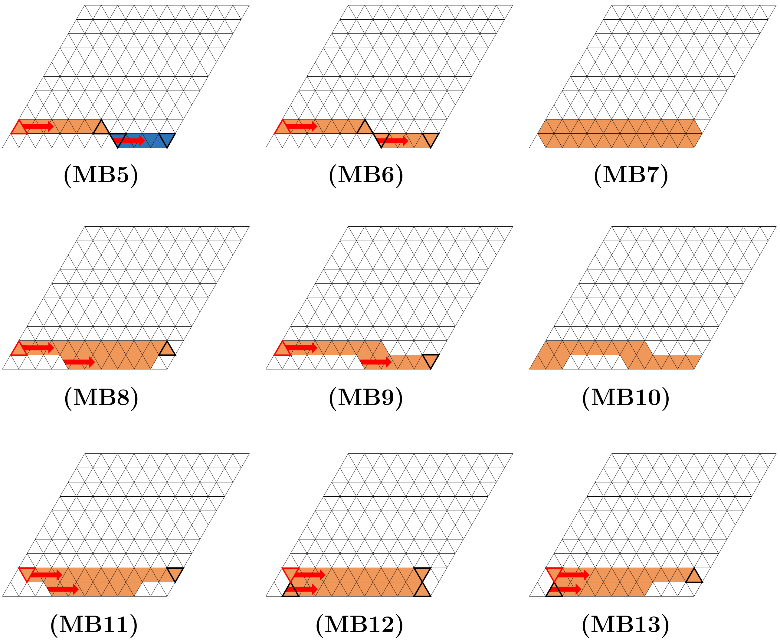
Figure 6.6. Types (MB5)-(MB13): We refer to the last part of the proof regarding the explanation of these figures.

To justify this classification, we first consider the case when $b_{1}\neq b_{2}$. Then, the $b_{1}$-protuberance in $\scal{h}_{1}$ and the $b_{2}$-protuberance in $\scal{h}_{2}$ must not be adjacent to each other, since otherwise there exists a vertical or diagonal non-semibridge strip. Since $\sigma$ is a cross-free configuration, we can readily conclude that $\sigma$ should be of type (MB5).

Next, we consider the case $b_{1}=b_{2}=b$ and we assume without loss of generality that the size of the $b$-protuberance in $\scal{h}_{2}$ is not smaller than that in $\scal{h}_{1}$. We can then divide the analysis into three subcases according to the shape of the $b$-protuberance in $\scal{h}_{2}$:

1. it has odd number of triangles and its lower side is longer than its upper side,

2. it has odd number of triangles and its upper side is longer than its lower side, or

3. it has even number of triangles.

Without loss of generality we assume that the $b$-protuberance in $\scal{h}_{2}$ is located at the leftmost part of the lattice as in Figure 6.6. For case (1), we can observe that the protuberance of $b$ in $\scal{h}_{1}$ also has odd number of triangles and its upper side should be longer than its lower side, since otherwise there will be a non-semibridge strip. According to five different types of locations of this protuberance in the strip $\scal{h}_{1}$, we get the types (MB6)-(MB10) illustrated in Figure 6.6. For case (2), we can similarly observe that the protuberance of $b$ in $\scal{h}_{1}$ also have odd number of triangles and it should be aligned as in (MB11) or (MB12). (In (MB12), $\scal{h}_{1}$ and $\scal{h}_{2}$ have the same size of $b$-protuberances.) Finally, for case (3), the $b$-protuberance in $\scal{h}_{1}$ should consist of even number of triangles and be aligned exactly as in (MB13). (In particular, it must be right-aligned.)

We have now fully characterized the configurations of type (MB), and it only remains to investigate the path-connectivity of types (MB6)-(MB13) to the configuration $\mathbf{a}$. We consider three cases separately.

• (MB10): Any update on this type of configuration increases the energy. Thus, those of this type satisfy $(\star\star)$.

• (MB7): We first flip a spin $a$ in $\scal{h}_{2}$ to spin $b$, so that we obtain a canonical configuration in $\mathcal{C}_{1}^{a,\,b}$ with protuberance size $2L-1$ (cf. Definition 6.5). Then, we can follow a canonical path (cf. Remark 6.7) from there to reach the configuration $\mathbf{a}$. The path associated with these updates is a $(2L+2)$-path of length $4L$. Moreover, $a$-bridges in $\scal{h}(\llbracket 3,\,L\rrbracket)$ are conserved along the path, and we can conclude that the configurations of this type satisfy $(\star)$.

• (MB5), (MB6), (MB8), (MB9), (MB11)-(MB13): We update spins $b$ to $a$ in the order indicated in Figure 6.6 to obtain the configuration $\mathbf{a}$. More precisely, for types (MB5), (MB6), (MB8), and (MB9), we update the triangles according to the indicated arrow starting from the one with red bold boundary to reach $\mathbf{a}$. For types (MB11)-(MB13), we first update the triangle with red bold boundary, then update one of the triangles with black bold boundary, and then update the remaining spins $b$ to $a$ according to the arrow to reach $\mathbf{a}$. In all the aforementioned types, one can select the starting triangle as the ones with black bold boundary. We remark that for (MB13), if there are same number of orange triangles in $\scal{h}_{1}$ and $\scal{h}_{2}$, then the black triangle at $\scal{h}_{2}$ is no longer available as a starting triangle. For (MB8), the red or black triangle might not be available as a starting triangle if the $b$-protuberance in $\scal{h}_{1}$ is aligned to the right or the left. Then, as in the previous case, we can readily observe that the path associated with these updates satisfies all the requirements in $(\star)$, and thus the configurations of these types satisfy $(\star)$.

This completes the proof. ∎

We can deduce the following lemma from a careful inspection of the proof of the previous lemma.

Lemma 6.16.

Let $\sigma\in\mathcal{X}$ be a configuration of type (MB) except (MB7) with parallel bridges of spin $a\in\Omega$, and let $\zeta\in\mathcal{X}$ be a configuration satisfying $\sigma\sim\zeta$ such that either $H(\zeta)\leq 2L+1$ or $\zeta$ has a cross. Then, there exists a $(2L+1)$-path of length less than $4L$ connecting $\zeta$ and $\mathbf{a}$. In particular, $\zeta\in\mathcal{N}(\mathbf{a})$.

Proof.

We can notice from Figures 6.5 and 6.6 that such a $\zeta$ exists only when $\sigma$ is of type (MB1)-(MB3), (MB5), (MB6), (MB8), (MB9), or (MB11)-(MB13), and moreover $\zeta$ is obtained from $\sigma$ by one of the following ways:

1. Updating the spin at a triangle highlighted by (either black or red) bold boundary in Figures 6.5 and 6.6 into $a$.

2. For type (MB3), $\zeta$ can be obtained by flipping spin $a$ at the strip $\scal{h}_{1}$ to $b$. For this case, $\zeta$ is a canonical configuration with $2L-1$ triangles of $b$ at a strip.

3. For type (MB8) such that the strip $\scal{h}_{1}$ contains only one triangle with spin $b$, the configuration $\zeta$ can additionally obtained by flipping that spin $b$ to spin $a$. We note that $\zeta$ is of the same type as in case (2) above.

For case (1), if $\zeta$ is obtained from $\sigma$ by flipping the spin at a triangle with red boundary, then we can continue to update according to the order indicated in the figure to reach $\mathbf{a}$. Then, the path corresponding to the sequence of updates provides a $(2L+1)$-path of length less than $4L$ connecting $\zeta$ and $\mathbf{a}$. The case when $\zeta$ is obtained from $\sigma$ by flipping a spin at a triangle with black boundary can be handled in a similar way. For cases (2) and (3), since $\zeta$ is a canonical configuration, it is connected to $\mathbf{a}$ via a canonical path (cf. Remark 6.7) which is a $(2L+1)$-path of length $2L-1$. ∎

Remark 6.17.

If we consider the Ising case, then the type (PP) is unavailable and also the analysis of type (MB) becomes much simpler.

As a byproduct of the characterization carried out in the current section, we derive a rough bound on the number of cross-free configurations which will be required in later computations. For a sequence $(a_{L})_{L=1}^{\infty}$, we write $a_{L}=O(f(L))$ if there exists a constant $C>0$ such that $|a_{L}|\leq Cf(L)$ for all $L$.

Lemma 6.18.

The number of cross-free configuration with energy less than or equal to $2L+2$ is $O(L^{6})$.

Proof.

Since we get a full characterization of cross-free configurations in Propositions 6.8, 6.11, and 6.13, the conclusion of the lemma follows directly from elementary counting. ∎

6.3. Dead-ends

In this subsection, we summarize the geometry of the energy landscape near the canonical configurations. As a consequence, we are able to get the full characterization of dead-ends (cf. Definition 6.22) the process encounters in the course of transitions between ground states.

We first introduce some notation.

• For a configuration $\sigma\in\mathcal{X}$ and $c\in\Omega$, we say that a subset $C$ of $\Lambda^{*}$ is a $c$-cluster if it is a monochromatic cluster consisting of spin $c$.

• The boundary of a set $A\subseteq\Lambda^{*}$ refers to the collection of triangles in $\Lambda^{*}\setminus A$ adjacent to triangles in $A$. An example is given by the following figure; if $A$ is the collection of orange triangles, the blue triangles are the boundary of $A$.

  

• For a configuration $\sigma\in\mathcal{X}$, we say that a triangle $x\in\Lambda^{*}$ is a boundary triangle of $\sigma$ if $x$ belongs to a boundary of a certain cluster of $\sigma$. Since a non-boundary triangle $x$ of $\sigma$ has the same spin with its three adjacent triangles, we can observe that

  $$\text{flipping the spin at a non-boundary triangle }x\text{ of }\sigma\text{ increases the energy by }3\;,$$ (6.5)

  while flipping the spin at a boundary triangle increases the energy by at most $2$ (or decreases the energy up to $3$).

• Let $\sigma\in\mathcal{X}$ be a configuration satisfying $H(\sigma)\leq 2L+2$. If $\zeta\in\mathcal{X}$ is obtained by a flip of spin of $\sigma$ (i.e., $\sigma\sim\zeta$) and $H(\zeta)\leq 2L+2$, we write $\sigma\approx\zeta$ and the corresponding flip is called a good flip.

We now characterize all the configurations connected to a canonical configuration $\sigma$ and having energy at most $2L+2$. We decompose our investigation into three cases: $\sigma\in\mathcal{R}_{n}^{a,\,b}$ (Lemma 6.19), $\sigma\in\mathcal{C}_{n,\,\scal{o}}^{a,\,b}$ (Lemma 6.20), and $\sigma\in\mathcal{C}_{n,\,\scal{e}}^{a,\,b}$ (Lemma 6.21). To that end, we define the following collections for $a,\,b\in\Omega$.

• $\mathcal{P}_{n}^{a,\,b}$, $n\in\llbracket 2,\,L-2\rrbracket$: the collection of configurations of type (PP) which can be obtained by a good flip of a configuration in $\mathcal{R}_{n}^{a,\,b}$.

• $\mathcal{Q}_{n}^{a,\,b}$, $n\in\llbracket 1,\,L-2\rrbracket$: the collection of configurations of type (ODP), (TDP), or (SP) which can be obtained by a good flip of a configuration in $\mathcal{C}_{n,\,\scal{o}}^{a,\,b}$.

• $\widehat{\mathcal{R}}_{n}^{a,\,b}$, $n\in\llbracket 2,\,L-2\rrbracket$: the collection of configurations $\zeta$ such that

  $$\text{either }\zeta\in\mathcal{C}_{n,\,\scal{o}}^{a,\,b}\text{ with }|\mathfrak{p}^{a,\,b}(\zeta)|=1\;,\text{ or }\zeta\in\mathcal{C}_{n-1,\,\scal{o}}^{a,\,b}\text{ with }|\mathfrak{p}^{a,\,b}(\zeta)|=2L-1\;.$$

  Namely, $\widehat{\mathcal{R}}_{n}^{a,\,b}$ is the collection of canonical configurations obtained by a good flip of a regular configuration in $\mathcal{R}_{n}^{a,\,b}$.

We now start the characterization. We fix $a,\,b\in\Omega$ in the remainder of the current section.

Lemma 6.19.

Suppose that $\sigma\in\mathcal{R}_{n}^{a,\,b}$ with $n\in\llbracket 2,\,L-2\rrbracket$ and $\zeta\in\mathcal{X}$ satisfies $\sigma\approx\zeta$. Then, we have either $\zeta\in\widehat{\mathcal{R}}_{n}^{a,\,b}$ or $\zeta\in\mathcal{P}_{n}^{a,\,b}$. In particular, we have $\widehat{\mathcal{R}}_{n}^{a,\,b}=\mathcal{N}(\mathcal{R}_{n}^{a,\,b})\setminus\mathcal{R}_{n}^{a,\,b}$.

Proof.

Let us fix $\sigma\in\mathcal{R}_{n}^{a,\,b}$. Since $H(\sigma)=2L$ and $H(\zeta)\leq 2L+2$, by (6.5), the configuration $\zeta$ is obtained from $\sigma$ by flipping a boundary triangle. First, we assume that we flip a spin at a boundary triangle of the $b$-cluster of $\sigma$ (which has spin $a$) to $c$ to get $\zeta$. As one can check from the figure below, we get $\zeta\in\widehat{\mathcal{R}}_{n}^{a,\,b}$ (in particular, $\zeta\in\mathcal{C}_{n,\,\scal{o}}^{a,\,b}$ with $|\mathfrak{p}^{a,\,b}(\zeta)|=1$) or $\zeta\in\mathcal{P}_{n}^{a,\,b}$ if $c=a$ or $c\notin\{a,\,b\}$, respectively.

The case when we flip a boundary triangle of the $a$-cluster is identical to the previous case and we can conclude the proof of the first statement. For the second statement, we first observe that if $\xi\sim\zeta$ for some $\zeta\in\widehat{\mathcal{R}}_{n}^{a,\,b}$ and $H(\xi)<2L+2$, then we must have $\xi\in\mathcal{R}_{n}^{a,\,b}$. Since the configuration of type (PP) has energy $2L+2$, the second assertion of the lemma is direct from the first one. ∎

Thanks to Lemma 6.19, we will hereafter discard the notation $\widehat{\mathcal{R}}_{n}^{a,\,b}$ and use $\mathcal{N}(\mathcal{R}_{n}^{a,\,b})\setminus\mathcal{R}_{n}^{a,\,b}$ instead.

Lemma 6.20.

Suppose that $\sigma\in\mathcal{C}_{n,\,\scal{o}}^{a,\,b}$ with $n\in\llbracket 2,\,L-2\rrbracket$ and $\zeta\in\mathcal{X}$ satisfies $\sigma\approx\zeta$. Then, we have either $\zeta\in\mathcal{R}_{n}^{a,\,b}\cup\mathcal{R}_{n+1}^{a,\,b}\cup\mathcal{C}_{n,\,\scal{e}}^{a,\,b}$, $\zeta\in\mathcal{P}_{n}^{a,\,b}\cup\mathcal{P}_{n+1}^{a,\,b}$, or $\zeta\in\mathcal{Q}_{n}^{a,\,b}$. In particular, if $3\leq|\mathfrak{p}^{a,\,b}(\sigma)|\leq 2L-3$, we have either $\zeta\in\mathcal{C}_{n,\,\scal{e}}^{a,\,b}$ or $\zeta\in\mathcal{Q}_{n}^{a,\,b}$.

Proof.

We fix $\sigma\in\mathcal{C}_{n,\,\scal{o}}^{a,\,b}$ and first consider the case $|\mathfrak{p}^{a,\,b}(\sigma)|=1$. By (6.5), we can notice that we have to flip a boundary triangle of $\sigma$ to get $\zeta$. We can group the boundary triangles of $\sigma$ into seven types as in Figure 6.7-(left).

Figure 6.7. Good flip of a configuration in $\mathcal{C}_{n,\,\scal{o}}^{a,\,b}$. (Left) $|\mathfrak{p}^{a,\,b}(\sigma)|=1$ or $2L-1$. (Right) $3\leq|\mathfrak{p}^{a,\,b}(\sigma)|\leq 2L-3$.

If we flip the triangle of type $1$, we get $\zeta\in\mathcal{R}_{n}^{a,\,b}$ or $\zeta\in\mathcal{P}_{n}^{a,\,b}$. If a flip of the spin of a triangle in types $2$-$7$ is a good flip, the spin must be flipped to either $a$ or $b$. Hence, we get a configuration in $\mathcal{C}_{n,\,\scal{e}}^{a,\,b}$ (resp. in $\mathcal{Q}_{n}^{a,\,b}$) if we flip the spin at a triangle of types $2$ or $3$ (resp. types $4$-$7$). The case $|\mathfrak{p}^{a,\,b}(\sigma)|=2L-1$ can be handled in the exact same way with this case and we get either $\zeta\in\mathcal{R}_{n+1}^{a,\,b}$, $\zeta\in\mathcal{P}_{n+1}^{a,\,b}$, $\zeta\in\mathcal{C}_{n,\,\scal{e}}^{a,\,b}$, or $\zeta\in\mathcal{Q}_{n}^{a,\,b}$.

Next, we consider the case $3\leq|\mathfrak{p}^{a,\,b}(\sigma)|\leq 2L-3$. The proof is similar to the previous case. In particular, the flip of triangles of types $2$-$7$ are of the identical nature. The only difference appears in the flip of a triangle of type $1$, i.e., a triangle in the protuberance of spin $b$. For this case, we have to flip triangle denoted by bold black boundary in Figure 6.7-(right) to get a configuration belonging to $\mathcal{C}_{n,\,\scal{e}}^{a,\,b}$ or $\mathcal{Q}_{n}^{a,\,b}$. ∎

Lemma 6.21.

Suppose that $\sigma\in\mathcal{C}_{n,\,\scal{e}}^{a,\,b}$ with $n\in\llbracket 2,\,L-2\rrbracket$ and $\zeta\in\mathcal{X}$ satisfies $\sigma\approx\zeta$. Then, $\zeta\in\mathcal{C}_{n,\,\scal{o}}^{a,\,b}$.

Proof.

There are essentially two cases (depending on whether the protuberance is connected or not) to be considered as in the figure below.

Since the configuration $\sigma$ already has energy $2L+2$, the good flip must not increase the energy, and therefore should flip the spin at one of the triangles with bold black boundary in the figure above either from $a$ to $b$ or from $b$ to $a$. Since the configuration obtained from this any of such flips belongs to $\mathcal{C}_{n,\,\scal{o}}^{a,\,b}$, the proof is completed. ∎

The non-canonical configurations appeared in the preceding three lemmas are defined now as the dead-ends.

Definition 6.22 (Dead-ends).

For $a,\,b\in\Omega$, define

$$\mathcal{D}^{a,\,b}=\Big{[}\,\bigcup_{n=2}^{L-2}\mathcal{P}_{n}^{a,\,b}\,\Big{]}\cup\Big{[}\,\bigcup_{n=2}^{L-3}\mathcal{Q}_{n}^{a,\,b}\,\Big{]}\;.$$

It is clear that $\sigma\in\mathcal{D}^{a,\,b}$ implies $H(\sigma)=2L+2$. We say that a configuration $\sigma$ belonging to $\mathcal{D}^{a,\,b}$ is a dead-end between $\mathbf{a}$ and $\mathbf{b}$. For each proper partition $(A,\,B)$, we write

$$\mathcal{D}^{A,\,B}=\bigcup_{a^{\prime}\in A}\bigcup_{b^{\prime}\in B}\mathcal{D}^{a^{\prime},\,b^{\prime}}\;.$$

Next, we perform further investigations on the dead-end configurations, after which we can explain why these configurations are called dead-ends (cf. Remark 6.26).

Lemma 6.23.

Suppose that $\sigma\in\mathcal{P}_{n}^{a,\,b}$ with $n\in\llbracket 2,\,L-2\rrbracket$ and $\zeta\in\mathcal{X}$ satisfies $\sigma\approx\zeta$. Then, we have either $\zeta\in\mathcal{N}(\mathcal{R}_{n}^{a,\,b})$ (two choices) or $\zeta\in\mathcal{P}_{n}^{a,\,b}$ ($q-3$ choices).

Proof.

A good flip of a configuration $\sigma\in\mathcal{P}_{n}^{a,\,b}$ must flip the spin at the peculiar protuberance. By flipping this spin to $a$ or $b$, we get a configuration in $\mathcal{N}(\mathcal{R}_{n}^{a,\,b})$. Otherwise, we get a configuration in $\mathcal{P}_{n}^{a,\,b}$ and we are done. ∎

Lemma 6.24.

Suppose that $\sigma\in\mathcal{Q}_{n}^{a,\,b}$ with $n\in\llbracket 2,\,L-3\rrbracket$ is obtained from $\xi\in\mathcal{C}_{n,\,\scal{o}}^{a,\,b}$ by flipping a spin. Suppose that $\zeta\in\mathcal{X}$ satisfies $\sigma\approx\zeta$.

1. If $|\mathfrak{p}^{a,\,b}(\xi)|\neq 1,\,2L-1$, we have $\zeta=\xi$.

2. If $|\mathfrak{p}^{a,\,b}(\xi)|=1$ (so that $\xi\in\mathcal{N}(\mathcal{R}_{n}^{a,\,b})$), there are exactly two possible configurations for $\zeta$, which are both in $\mathcal{N}(\mathcal{R}_{n}^{a,\,b})\setminus\mathcal{R}_{n}^{a,\,b}$.

3. If $|\mathfrak{p}^{a,\,b}(\xi)|=2L-1$ (so that $\xi\in\mathcal{N}(\mathcal{R}_{n+1}^{a,\,b})$), there are exactly two possible configurations for $\zeta$, which are both in $\mathcal{N}(\mathcal{R}_{n+1}^{a,\,b})\setminus\mathcal{R}_{n+1}^{a,\,b}$.

Proof.

If $|\mathfrak{p}^{a,\,b}(\xi)|\neq 1,\,2L-1$. we can notice from the figure below that $\sigma$ is obtained from $\xi$ by flip the spin at one of the triangles with bold boundary either from $a$ to $b$ or $b$ to $a$.

Then, it is direct from that a good flip of $\sigma$ must flip back this updated spin, since otherwise the energy will be further increased to at least $2L+3$. Hence, we get $\zeta=\xi$.

Next, we consider the case $|\mathfrak{p}^{a,\,b}(\xi)|=1$. Then, as in the figure below, $\sigma$ should be obtained by adding a protuberance of spin $a$ or $b$ of size one to $\xi$, and there are four different types.

Therefore, $\sigma$ has two protuberances of size one denoted by bold boundary and a good flip must remove one of them. Thus, there are exactly two possible configurations $\zeta_{1},\,\zeta_{2}$ for $\zeta$ and it is immediate that $\zeta_{1},\,\zeta_{2}\in\mathcal{N}(\mathcal{R}_{n}^{a,\,b})\setminus\mathcal{R}_{n}^{a,\,b}$. The proof for the case $|\mathfrak{p}^{a,\,b}(\xi)|=2L-1$ is almost identical to the case $|\mathfrak{p}^{a,\,b}(\xi)|=1$ and we omit the detail. ∎

Finally, we provide a summary of the preceding results.

Proposition 6.25.

Let $\sigma\in\bigcup_{n=2}^{L-3}\mathcal{C}_{n}^{a,\,b}$ or $\sigma\in\mathcal{D}^{a,\,b}$ and suppose that $\zeta\in\mathcal{X}$ satisfies $\zeta\approx\sigma$. Then, $\zeta$ is either a canonical configuration or a dead-end in $\mathcal{D}^{a,\,b}$.

Proof.

This proposition is a direct consequence of Lemmas 6.19, 6.20, 6.21, 6.23, and 6.24. ∎

Remark 6.26.

Now, we are able to explain why the configurations in $\mathcal{D}^{a,\,b}$ is called dead-end configurations. According to the definition of $\mathcal{D}^{a,\,b}$, a dead-end $\sigma$ is adjacent to either $\mathcal{N}(\mathcal{R}_{n}^{a,\,b})$ for some $n\in\llbracket 2,\,L-2\rrbracket$ or $\xi\in\mathcal{C}_{n,\,\scal{o}}^{a,\,b}$ such that $|\mathfrak{p}^{a,\,b}(\xi)|\in\llbracket 3,\,2L-3\rrbracket$ for some $n\in\llbracket 2,\,L-3\rrbracket$. Let $\sigma\approx\zeta$. Then, for the former case, by Lemmas 6.23 and 6.24-(2)(3), $\zeta$ is either another dead-end configuration adjacent to $\mathcal{N}(\mathcal{R}_{n}^{a,\,b})$ or a configuration in $\mathcal{N}(\mathcal{R}_{n}^{a,\,b})$. Hence, these ones indeed serve as dead-ends attached to $\mathcal{N}(\mathcal{R}_{n}^{a,\,b})$ (which consists of canonical configurations only by Lemma 6.19). For the latter case, $\zeta=\xi$ by Lemma 6.24-(1) and therefore $\{\sigma\}$ is a single dead-end attached to the canonical configuration $\xi$.

6.4. Energy barrier

Now, we are ready to prove Theorem 3.1. We first establish the upper bound.

Proposition 6.27.

For any $a,\,b\in\Omega$, we have $\Phi(\mathbf{a},\,\mathbf{b})\leq 2L+2$.

Proof.

Let $P_{0}=\emptyset$ and let $P_{n}=\{1,\,\dots,\,n\}\subseteq\mathbb{T}_{L}$ for $n\in\llbracket 1,\,L\rrbracket$ so that $P_{0}\prec P_{1}\prec\cdots\prec P_{L}$. Since $\xi_{\scal{h}(P_{0})}^{a,\,b}=\mathbf{a}$ and $\xi_{\scal{h}(P_{L})}^{a,\,b}=\mathbf{b}$, it suffices to show that $\Phi(\xi_{\scal{h}(P_{n})}^{a,\,b},\,\xi_{\scal{h}(P_{n+1})}^{a,\,b})\leq 2L+2$ for all $n\in\llbracket 0,\,L-1\rrbracket$. This follows from Remark 6.7. ∎

Next, we turn to the matching lower bound which is the crucial part in the proof.

Proposition 6.28.

For any $a,\,b\in\Omega$, we have $\Phi(\mathbf{a},\,\mathbf{b})\geq 2L+2$.

Proof.

Suppose the contrary so that there exists a $(2L+1)$-path $(\omega_{n})_{n=0}^{N}$ in $\mathcal{X}$ with $\omega_{0}=\mathbf{a}$, $\omega_{N}=\mathbf{b}$. For each $n\in\llbracket 0,\,N\rrbracket$, define $u(n)$ as the number of $b$-bridges in $\omega_{n}$ so that we have $u(0)=0$ and $u(N)=3L$. Now, we define

$$n^{*}=\min\{n\in\llbracket 0,\,N\rrbracket:u(n)\geq 2\}\;,$$ (6.6)

so that we have a trivial bound $n^{*}\geq 3$. Notice that a spin flip at a certain triangle can only affect the three strips containing that triangle and hence

$$|u(n+1)-u(n)|\leq 3\;\;\;\;\text{for all}\;n\in\llbracket 0,\,L-1\rrbracket\;.$$ (6.7)

From this observation, we know that $u(n^{*})\in\llbracket 2,\,4\rrbracket$. On the other hand, by Lemma 5.3, we have at least $3L-(2L+1)=L-1$ bridges, and hence there exists a bridge with spin not $b$. This implies that $\omega_{n^{*}}$ does not have a cross. Then, we must have $u(n^{*})-u(n^{*}-1)=1$ and therefore we have $u(n^{*})=2$.

By Propositions 6.8 and 6.11, we have either $\omega_{n^{*}}\in\mathcal{R}_{2}^{a^{\prime},\,b}$ or $\omega_{n^{*}}\in\mathcal{C}_{2,\,\scal{o}}^{a^{\prime},\,b}$ for some $a^{\prime}\in\Omega\setminus\{b\}$. If $\omega_{n^{*}}\in\mathcal{R}_{2}^{a^{\prime},\,b}$, then by Lemma 6.19 and the minimality assumption of $n^{*}$, we must have $\omega_{n^{*}-1}\in\mathcal{C}_{1,\,\scal{o}}^{a^{\prime},\,b}$. Then, since $H(\omega_{n^{*}-2})\leq 2L+1$, we can deduce from Lemma 6.20 that $\omega_{n^{*}-2}\in\mathcal{R}_{2}^{a^{\prime},\,b}$ which contradicts the minimality of $n^{*}$ in (6.6). On the other hand, if $\omega_{n^{*}}\in\mathcal{C}_{2,\,\scal{o}}^{a^{\prime},\,b}$, then since $H(\omega_{n^{*}-1})\leq 2L+1$, we can infer from Lemma 6.20 that $\omega_{n^{*}-1}\in\mathcal{R}_{2}^{a^{\prime},\,b}\cup\mathcal{R}_{3}^{a^{\prime},\,b}$, and therefore we again get a contradiction to the minimality of $n^{*}$. Since we got a contradiction for both cases, the proof is completed. ∎

Now, we can conclude the proof of Theorem 3.1.

Proof of Theorem 3.1.

By Propositions 6.27 and 6.28, it suffices to prove that $\Phi(\sigma,\,\mathcal{S})-H(\sigma)<2L+2$ for all $\sigma\notin\mathcal{S}$. The proof of this bound is identical to [20, Lemma 6.11] and we refer to the detailed proof therein. ∎

7. Saddle Structure

In order to get the Eyring–Kramers-type quantitative analysis of metastability, we need more detailed understanding of the energy landscape. We perform this in the current section by completely analyzing the saddle structure between ground states. We remark that the discussion given in this section has similar flavor with that of [20, Section 7], but the detail is quite different because we are considering hexagonal lattice with a complicated dead-end structure, and also we are working on the large volume regime.

7.1. Typical configurations

Definition 7.1 (Typical configurations).

Let $(A,\,B)$ be a proper partition of $\Omega$.

1. For $a,\,b\in\Omega$, we define the collection of bulk typical configurations between $\mathbf{a}$ and $\mathbf{b}$ as

   $$\mathcal{B}^{a,\,b}=\bigcup_{n=2}^{L-3}\mathcal{C}_{n}^{a,\,b}\cup\mathcal{D}^{a,\,b}\;.$$ (7.1)

   Then, we define the collection of bulk configurations between $\mathcal{S}(A)$ and $\mathcal{S}(B)$ as

   $$\mathcal{B}^{A,\,B}=\bigcup_{a^{\prime}\in A}\bigcup_{b^{\prime}\in B}\mathcal{B}^{a^{\prime},\,b^{\prime}}\;.$$

2. For $a,\,b\in\Omega$, we write

   $$\mathcal{B}_{\Gamma}^{a,\,b} =\{\sigma\in\mathcal{B}^{a,\,b}:H(\sigma)=\Gamma\}=\bigcup_{n=2}^{L-3}\mathcal{C}_{n,\,\scal{e}}^{a,\,b}\cup\mathcal{D}^{a,\,b}\;,$$

   $$\mathcal{B}_{\Gamma}^{A,\,B} =\{\sigma\in\mathcal{B}^{A,\,B}:H(\sigma)=\Gamma\}=\bigcup_{a^{\prime}\in A}\bigcup_{b^{\prime}\in B}\mathcal{B}_{\Gamma}^{a^{\prime},\,b^{\prime}}\;.$$

   Then, we define (cf. Definition 5.4)

   $$\mathcal{E}^{A}=\widehat{\mathcal{N}}\big{(}\,\mathcal{S}(A);\,\mathcal{B}_{\Gamma}^{A,\,B}\,\big{)}\;\;\;\;\text{and}\;\;\;\;\mathcal{E}^{B}=\widehat{\mathcal{N}}\big{(}\,\mathcal{S}(B);\,\mathcal{B}_{\Gamma}^{A,\,B}\,\big{)}\;.$$ (7.2)

   The collection of edge typical configurations between $\mathcal{S}(A)$ and $\mathcal{S}(B)$ is defined as

   $$\mathcal{E}^{A,\,B}=\mathcal{E}^{A}\cup\mathcal{E}^{B}\;.$$

In the remainder of the current section, we fix a proper partition $(A,\,B)$ of $\Omega$.

Remark 7.2.

In fact, all canonical configurations are indeed typical configurations. To see this, we let $c_{1},\,c_{2}\in\Omega$ and demonstrate that $\mathcal{C}_{n}^{c_{1},\,c_{2}}\subseteq\mathcal{B}^{A,\,B}\cup\mathcal{E}^{A,\,B}$ for all $n\in\llbracket 0,\,L-1\rrbracket$. First, if $c_{1},\,c_{2}\in A$ or $c_{1},\,c_{2}\in B$, then by Remark 6.7, it is straightforward that $\mathcal{C}_{n}^{c_{1},\,c_{2}}\subseteq\mathcal{E}^{A}$ or $\mathcal{C}_{n}^{c_{1},\,c_{2}}\subseteq\mathcal{E}^{B}$, respectively. Next, we assume that $c_{1}$ and $c_{2}$ belong to different sets, say $c_{1}\in A$ and $c_{2}\in B$. We divide into two cases.

1. In the bulk part, for $n\in\llbracket 2,\,L-3\rrbracket$ we have $\mathcal{C}_{n}^{c_{1},\,c_{2}}\subseteq\mathcal{B}^{A,\,B}$ which is immediate from the definition (7.1).

2. Remarks 6.6 and 6.7 imply that all the canonical configurations in $\mathcal{C}_{0}^{c_{1},\,c_{2}}\cup\mathcal{C}_{1}^{c_{1},\,c_{2}}$ are connected by a $\Gamma$-path in $\mathcal{C}_{0}^{c_{1},\,c_{2}}\cup\mathcal{C}_{1}^{c_{1},\,c_{2}}$ to $\mathbf{c_{1}}\in\mathcal{S}(A)$. As we clearly have $(\mathcal{C}_{0}^{c_{1},\,c_{2}}\cup\mathcal{C}_{1}^{c_{1},\,c_{2}})\cap\mathcal{B}_{\Gamma}^{A,\,B}=\emptyset$, the definition of $\mathcal{E}^{A}$ implies that $\mathcal{C}_{0}^{c_{1},\,c_{2}}\cup\mathcal{C}_{1}^{c_{1},\,c_{2}}\subseteq\mathcal{E}^{A}$. Similarly, we have $\mathcal{C}_{L-2}^{c_{1},\,c_{2}}\cup\mathcal{C}_{L-1}^{c_{1},\,c_{2}}\subseteq\mathcal{E}^{B}$.

Proposition 7.3.

The following properties hold.

1. We have $\mathcal{E}^{A}\cap\mathcal{B}^{A,\,B}=\mathcal{N}(\mathcal{R}_{2}^{A,\,B})$ and $\mathcal{E}^{B}\cap\mathcal{B}^{A,\,B}=\mathcal{N}(\mathcal{R}_{L-2}^{A,\,B})$.

2. It holds that $\mathcal{E}^{A,\,B}\cup\mathcal{B}^{A,\,B}=\widehat{\mathcal{N}}(\mathcal{S})$.

This proposition explains why we defined the typical configurations as in Definition 7.1. In particular, since $\widehat{\mathcal{N}}(\mathcal{S})$ is the collection of all configurations connected to the ground states by a $\Gamma$-path, we can observe from part (2) of the previous proposition that the sets $\mathcal{E}^{A,\,B}$ and $\mathcal{B}^{A,\,B}$ are properly defined to explain the saddle structure between $\mathcal{S}(A)$ and $\mathcal{S}(B)$.

The proof of Proposition 7.3 is identical to that of [20, Proposition 7.5], since the proof therein is robust against the microscopic feature of the model. It suffices to replace [20, Lemma 7.2] for the square lattice with Lemmas 6.19, 6.20, and 6.21 for the hexagonal lattice. It should be mentioned that in [20, Proposition 7.5], it was asserted that $\mathcal{E}^{A}\cap\mathcal{B}^{A,\,B}=\mathcal{R}_{2}^{A,\,B}$ and $\mathcal{E}^{B}\cap\mathcal{B}^{A,\,B}=\mathcal{R}_{L-2}^{A,\,B}$ (instead of $\mathcal{N}(\mathcal{R}_{2}^{A,\,B})$ and $\mathcal{N}(\mathcal{R}_{L-2}^{A,\,B})$) since in that case it holds that $\mathcal{N}(\mathcal{R}_{i}^{A,\,B})=\mathcal{R}_{i}^{A,\,B}$ for all $i\in\llbracket 2,\,L-2\rrbracket$.

The following proposition is the hexagonal version of [20, Proposition 7.4] and asserts that $\mathcal{E}^{A}$ and $\mathcal{E}^{B}$ are disjoint. We provide a proof since it is technically more difficult than that of [20, Proposition 7.4]. A union of two strips of different directions is called a $b$-semicross of $\sigma\in\mathcal{X}$ if all the spins at these two strips are $b$, except for the one in the intersection which is not $b$, as in the following figure.

Proposition 7.4.

Let $(A,\,B)$ be a proper partition. Each configuration in $\mathcal{E}^{A}$ does not have a $b$-cross for all $b\in B$. In particular, it holds that $\mathcal{E}^{A}\cap\mathcal{E}^{B}=\emptyset$.

Proof.

Suppose on the contrary that $\sigma\in\mathcal{E}^{A}$ has a $b$-cross for some $b\in B$. Then since $\sigma\in\mathcal{E}^{A}$, we can find a $\Gamma$-path $(\omega_{n})_{n=0}^{N}$ in $\mathcal{X}\setminus\mathcal{B}_{\Gamma}^{A,\,B}$ with $\omega_{0}\in\mathcal{S}(A)$ and $\omega_{N}=\sigma$. For $n\in\llbracket 0,\,N\rrbracket$, define $u(n)$ as the number of $b$-bridges in $\omega_{n}$ so that

$$u(0)=0\;,\;u(N)\geq 2\;,\;\text{and }|u(n+1)-u(n)|\leq 3\text{ for all }n\in\llbracket 0,\,N-1\rrbracket\;,$$ (7.3)

as in the proof of Proposition 6.28. Define

$$n_{0}=\max\{n\geq 1:u(n-1)\leq 1\text{ and }u(n)\geq 2\}$$

so that, summing up,

$$(\omega_{n})_{n=0}^{N}\text{ is a }\Gamma\text{-path in }\mathcal{X}\setminus\mathcal{B}_{\Gamma}^{A,\,B}\;\;\;\;\text{and}\;\;\;\;u(n)\geq 2\text{ for all }n\geq n_{0}\;.$$ (7.4)

We divide the proof into two cases.

(Case 1: $u(n_{0})-u(n_{0}-1)\geq 2$) In this case, a single spin update from $\omega_{n_{0}-1}$ to $\omega_{n_{0}}$ creates at least two $b$-bridges. This is possible only when we update the triangle at the intersection of a $b$-semicross to obtain a $b$-cross. Since $u(n_{0}-1)\in\{0,\,1\}$, the configuration $\omega_{n_{0}-1}$ cannot have a $b$-cross. Moreover, the existence of a $b$-semicross implies that there is no $c$-bridge for all $c\in\Omega\setminus\{b\}$. Hence, $\omega_{n_{0}-1}$ has at most one bridge and its energy is at least $3L-1$ by Lemma 5.3. This contradicts the fact that $(\omega_{n})$ is a $\Gamma$-path.

(Case 2: $u(n_{0})-u(n_{0}-1)=1$) Here, we must have $u(n_{0}-1)=1$ and $u(n_{0})=2$. Since $\omega_{n_{0}-1}$ has exactly one $b$-bridge, it is cross-free. Moreover, since a single spin update from $\omega_{n_{0}-1}$ to $\omega_{n_{0}}$ should create the second $b$-bridge, we can apply Propositions 6.8, 6.11, and 6.13 to assert that there are only four possible forms of $\omega_{n_{0}-1}$ as in the figure below.

Note that we have to update the spin at a triangle with bold boundary to $b$ to get $\omega_{n_{0}},$and hence we have $\omega_{n_{0}}\in\mathcal{R}_{2}^{a,\,b}\cup\mathcal{C}_{2,\,\scal{o}}^{a,\,b}$. Note that $\omega_{n_{0}}$ does not have a $b$-cross so that $n_{0}<N$. Now, we consider four subcases.

• $\omega_{n_{0}}\in\mathcal{R}_{2}^{a,\,b}$: We can conclude from Lemmas 6.19, 6.20, 6.23, and 6.24-(2) along with (7.4) that $\omega_{n}\in\mathcal{N}(\mathcal{R}_{2}^{a,\,b})$ for all $n\geq n_{0}$. This contradicts the fact that $\omega_{N}$ has a $b$-cross.

• $\omega_{n_{0}}\in\mathcal{C}_{2,\,\scal{o}}^{a,\,b}$ with $|\mathfrak{p}^{a,\,b}(\omega_{n_{0}})|\in\llbracket 3,\,2L-3\rrbracket$: Since $\omega_{n_{0}}\approx\omega_{n_{0}+1}$, by Lemma 6.20, we get $\omega_{n_{0}+1}\in\mathcal{C}_{2,\,\scal{e}}^{a,\,b}\cup\mathcal{Q}_{2}^{a,\,b}\subseteq\mathcal{B}_{\Gamma}^{A,\,B}$. This contradicts (7.4).

• $\omega_{n_{0}}\in\mathcal{C}_{2,\,\scal{o}}^{a,\,b}$ with $|\mathfrak{p}^{a,\,b}(\omega_{n_{0}})|=1$: The same logic with the case $\omega_{n_{0}}\in\mathcal{R}_{2}^{a,\,b}$ leads to the same conclusion.

• $\omega_{n_{0}}\in\mathcal{C}_{2,\,\scal{o}}^{a,\,b}$ with $|\mathfrak{p}^{a,\,b}(\omega_{n_{0}})|=2L-1$: By the same logic with the case $\omega_{n_{0}}\in\mathcal{R}_{2}^{a,\,b}$, we get $\omega_{n}\in\mathcal{N}(\mathcal{R}_{3}^{a,\,b})$ for all $n\geq n_{0}$. This again contradicts the fact that $\omega_{N}$ has a $b$-cross.

Since we get a contradiction for all cases, the first assertion of the proposition is proved. For the second assertion, we first observe from the first part of the proposition that $\mathcal{E}^{A}\cap\mathcal{S}(B)=\emptyset$. Then, by the definitions of $\mathcal{E}^{A}$ and $\mathcal{E}^{B}$, it also holds that $\mathcal{E}^{A}\cap\mathcal{E}^{B}=\emptyset$. ∎

7.2. Structure of edge configurations

Fix a proper partition $(A,\,B)$ throughout this subsection. We now investigate the structure of the sets $\mathcal{E}^{A}$ and $\mathcal{E}^{B}$ more deeply as in [20, Section 7.3].

We start by decomposing $\mathcal{E}^{A}=\mathcal{I}^{A}\cup\mathcal{O}^{A}$ where

$$\mathcal{O}^{A}=\{\sigma\in\mathcal{E}^{A}:H(\sigma)=\Gamma\}\;\;\;\;\text{and}\;\;\;\;\mathcal{I}^{A}=\{\sigma\in\mathcal{E}^{A}:H(\sigma)<\Gamma\}\;.$$

Further, we take a representative set $\mathcal{I}_{\textup{rep}}^{A}\subseteq\mathcal{I}^{A}$ in such a way that each $\sigma\in\mathcal{I}^{A}$ satisfies $\sigma\in\mathcal{N}(\zeta)$ for exactly one $\zeta\in\mathcal{I}_{\textup{rep}}^{A}$. With this notation, we can further decompose the set $\mathcal{E}^{A}$ into

$$\mathcal{E}^{A}=\mathcal{O}^{A}\cup\Big{(}\,\bigcup_{\zeta\in\mathcal{I}_{\textup{rep}}^{A}}\mathcal{N}(\zeta)\,\Big{)}\;.$$

For the convenience of notation, we can assume that $\mathcal{S}(A),\,\mathcal{R}_{2}^{A,\,B}\subseteq\mathcal{I}_{\textup{rep}}^{A}$ so that configurations in $\mathcal{N}(\mathbf{a})$ with $\mathbf{a}\in\mathcal{S}(A)$ and in $\mathcal{N}(\sigma)$ with $\sigma\in\mathcal{R}_{2}^{A,\,B}$ are represented by $\mathbf{a}$ and $\sigma$, respectively.

We now assign a graph structure on $\mathcal{E}^{A}$ based on this decomposition. More precisely, we introduce a graph $\mathscr{G}^{A}=(\mathscr{V}^{A},\,E(\mathscr{V}^{A}))$ where the vertex set is defined by $\mathscr{V}^{A}=\mathcal{O}^{A}\cup\mathcal{I}_{\textup{rep}}^{A}$ and the edge set is defined by $\{\sigma,\,\sigma^{\prime}\}\in E(\mathscr{V}^{A})$ for $\sigma,\,\sigma^{\prime}\in\mathscr{V}^{A}$ if and only if

$$\begin{cases}\sigma,\,\sigma^{\prime}\in\mathcal{O}^{A}\text{ and }\sigma\sim\sigma^{\prime}\;\;\text{or}\\ \sigma\in\mathcal{O}^{A}\;,\;\sigma^{\prime}\in\mathcal{I}_{\textup{rep}}^{A}\text{ and }\sigma\sim\zeta\text{ for some }\zeta\in\mathcal{N}(\sigma^{\prime})\;.\end{cases}$$

Next, we construct a continuous-time Markov chain $\{Z^{A}(t)\}_{t\geq 0}$ on $\mathscr{V}^{A}$ with rate $r^{A}:\mathscr{V}^{A}\times\mathscr{V}^{A}\rightarrow\mathbb{R}$ defined by

$$r^{A}(\sigma,\,\sigma^{\prime})=\begin{cases}1&\text{if }\sigma,\,\sigma^{\prime}\in\mathcal{O}^{A}\;,\\ |\{\zeta\in\mathcal{N}(\sigma):\zeta\sim\sigma^{\prime}\}|&\text{if }\sigma\in\mathcal{I}_{\textup{rep}}^{A}\;,\;\sigma^{\prime}\in\mathcal{O}^{A}\;,\\ |\{\zeta\in\mathcal{N}(\sigma^{\prime}):\zeta\sim\sigma\}|&\text{if }\sigma\in\mathcal{O}^{A}\;,\;\sigma^{\prime}\in\mathcal{I}_{\textup{rep}}^{A}\;,\end{cases}$$ (7.5)

and $r^{A}(\sigma,\,\sigma^{\prime})=0$ if $\{\sigma,\,\sigma^{\prime}\}\notin E(\mathscr{V}^{A})$. Since the rate $r^{A}(\cdot,\,\cdot)$ is symmetric, the Markov chain $Z^{A}(\cdot)$ is reversible with respect to the uniform distribution on $\mathscr{V}^{A}$.

Notation 7.5.

We denote by $L^{A}(\cdot)$, $h_{\cdot,\,\cdot}^{A}(\cdot)$, $\mathrm{cap}^{A}(\cdot,\,\cdot)$, and $D^{A}(\cdot)$ the generator, equilibrium potential, capacity, and Dirichlet form, respectively, of the Markov chain $Z^{A}(\cdot)$. For those who are not familiar with these notions, we refer to Section 8.1 for the definitions.

Configurations in $\mathcal{E}^{A}$

In the following series of lemmas, we study several essential features of the configurations in $\mathcal{E}^{A}$.

Lemma 7.6.

Suppose that $\sigma\in\mathcal{E}^{A}$ has an $a$-cross for some $a\in A$. Then, we have that $h_{\mathcal{S}(A),\,\mathcal{R}_{2}^{A,B}}^{A}(\sigma)=1$ (cf. Notation 7.5).

Proof.

We fix $\sigma\in\mathcal{E}^{A}$ which has an $a$-cross for some $a\in A$. It suffices to prove that any $\Gamma$-path from $\sigma$ to $\mathcal{R}_{2}^{A,\,B}$ in $\mathcal{X}\setminus\mathcal{B}_{\Gamma}^{A,\,B}$ must visit $\mathcal{N}(\mathcal{S}(A))$. Suppose the contrary that there exists a $\Gamma$-path $(\omega_{n})_{n=0}^{N}$ in $\mathcal{X}\setminus[\mathcal{N}(\mathcal{S}(A))\cup\mathcal{B}_{\Gamma}^{A,\,B}]$ connecting $\omega_{0}\in\mathcal{R}_{2}^{A,\,B}$ and $\omega_{N}=\sigma$. Let

$$n_{1}=\min\{n\geq 1:\omega_{n}\text{ has an }a\text{-cross}\}\in\llbracket 1,\,N\rrbracket\;,$$

so that $\omega_{n_{1}-1}$ is clearly cross-free. Hence, we are able to apply Propositions 6.8, 6.11, and 6.13 to conclude that $\omega_{n_{1}-1}$ is either of type (MB) or satisfies $\omega_{n_{1}-1}\in\mathcal{C}_{0,\,\scal{o}}^{a,\,b}$ with $|\mathfrak{p}^{a,\,b}(\omega_{n_{1}-1})|=2L-1$. For the former case, $\omega_{n_{1}-1}$ is clearly not of type (MB7) since $\omega_{n_{1}}$ must have a cross, and thus by Lemma 6.16, we have $\omega_{n_{1}}\in\mathcal{N}(\mathbf{a})$ and we get a contradiction. For the latter case, since $\omega_{n_{1}}$ has an $a$-cross, the configurations $\omega_{n_{1}-1}$ and $\omega_{n_{1}}$ must be of the following form.

Thus, we update each spin $b$ in $\omega_{n_{1}}$ to spin $a$ in a consecutive manner as in the proof of Lemma 6.15 (where we start the update from a triangle highlighted by bold boundary) to get a $(\Gamma-1)$-path from $\omega_{n_{1}}$ to $\mathbf{a}$. Hence, we have $\omega_{n_{1}}\in\mathcal{N}(\mathbf{a})$ and we get a contradiction for this case as well. ∎

Lemma 7.7.

Fix $a\in A$ and suppose that $\sigma\in\mathcal{N}(\mathbf{a})$ and that there exists $\zeta\in\mathcal{O}^{A}$ such that $\sigma\sim\zeta$ and $h_{\mathcal{S}(A),\,\mathcal{R}_{2}^{A,B}}^{A}(\zeta)\neq 1$. Then, the followings hold.

1. There exists a $(\Gamma-1)$-path from $\sigma$ to $\mathbf{a}$ of length less than $4L$.

2. We have

   $$\big{|}\,\{\sigma\in\mathcal{N}(\mathbf{a}):\exists\zeta\in\mathcal{O}^{A}\text{ with }\sigma\sim\zeta\text{ and }h_{\mathcal{S}(A),\,\mathcal{R}_{2}^{A,B}}^{A}(\zeta)\neq 1\}\,\big{|}=O(L^{8})\;.$$

Proof.

(1) By Proposition 7.4 and Lemma 7.6, $\zeta$ is a cross-free configuration of energy $\Gamma$. Thus, by Proposition 6.13, $\zeta$ is of type (ODP), (TDP), (SP), (EP), (PP) or (MB). For the first five types, since $\sigma\in\mathcal{N}(\mathbf{a})$, we can readily infer that the only possible cases are $\sigma\in\mathcal{R}_{1}^{a,\,c}$ or $\sigma\in\mathcal{C}_{1,\,\scal{o}}^{a,\,c}$ with $|\mathfrak{p}^{a,\,c}(\sigma)|=1$ for some $c\in\Omega\setminus\{a\}$. Then, we clearly have a $(\Gamma-1)$-path from $\sigma$ to $\mathbf{a}$ of length $2L$ or $2L+1$ which is indeed a canonical path (cf. Remarks 6.6 and 6.7). Next we assume that $\zeta$ is of type (MB). If $\zeta$ is of type (MB7), then clearly we have $\sigma\in\mathcal{C}_{1,\,\scal{o}}^{c,\,c^{\prime}}$ for some $c,\,c^{\prime}\in\Omega$, which contradicts $\sigma\in\mathcal{N}(\mathbf{a})$ by Lemmas 6.19 and 6.20. Otherwise, the statement of part (1) is direct from Lemma 6.16.

(2) Since $\zeta$ is a cross-free configuration of energy $\Gamma$, Lemma 6.18 implies that there are $O(L^{6})$ possibilities for $\zeta$. As there are $O(L^{2})$ ways of flipping a spin, we get a (loose) bound $O(L^{8})$ for the number of possible configurations for $\sigma$. ∎

Lemma 7.8.

Let $\zeta\in\mathcal{I}_{\textup{rep}}^{A}\setminus(\mathcal{S}(A)\cup\mathcal{R}_{2}^{A,\,B}\cup\mathcal{C}_{1,\,\scal{o}}^{A,\,B})$ and let $\sigma\in\mathcal{N}(\zeta)$. Then, $\sigma$ has an $a$-cross for some $a\in A$. If $\xi\in\mathcal{O}^{A}$ satisfies $\xi\sim\sigma$, then $\xi$ also has an $a$-cross.

Proof.

By Propositions 6.8 and 6.11, $\sigma$ cannot be a cross-free configuration. Since $\sigma$ cannot have a $b$-cross for $b\in B$ by Proposition 7.4, it must have an $a$-cross for some $a\in A$. For the second part of the lemma, since $\xi\sim\sigma$, the configuration $\xi$ should be cross-free if it does not have an $a$-cross. If $\xi$ is cross-free, then by Proposition 6.13, $\xi$ is of type (ODP), (TDP), (SP), (EP), (PP) or (MB). The first five types are impossible since $\sigma$ has a cross. If $\xi$ is of type (MB) other than (MB7), then Lemma 6.16 implies that $\sigma\in\mathcal{N}(\mathbf{a})$ which contradicts $\zeta\notin\mathcal{S}(A)$. Finally, if $\xi$ is of type (MB7), then $\sigma$ cannot have a cross, and thus we have a contradiction. This concludes the proof. ∎

Estimate of jump rate

The following proposition explains the reason why we introduced the Markov chain $Z^{A}(\cdot)$.

Proposition 7.9.

Define a projection map $\Pi^{A}:\mathcal{E}^{A}\rightarrow\mathscr{V}^{A}$ by

$$\Pi^{A}(\sigma)=\begin{cases}\zeta&\text{if }\sigma\in\mathcal{N}(\zeta)\text{ for some }\zeta\in\mathcal{I}_{\textup{rep}}^{A}\;,\\ \sigma&\text{if }\sigma\in\mathcal{O}^{A}\;.\end{cases}$$

Suppose that $L^{2/3}\ll e^{\beta}$. Then, the followings hold.

1. For $\sigma_{1},\,\sigma_{2}\in\mathcal{O}^{A}$ with $\sigma_{1}\sim\sigma_{2}$, we have

   $$\frac{1}{q}e^{-\Gamma\beta}r^{A}\big{(}\,\Pi^{A}(\sigma_{1}),\,\Pi^{A}(\sigma_{2})\,\big{)}=(1+o_{L}(1))\times\mu_{\beta}(\sigma_{1})c_{\beta}(\sigma_{1},\,\sigma_{2})\;.$$

2. For $\sigma_{1}\in\mathcal{O}^{A}$ and $\sigma_{2}\in\mathcal{I}^{A}$ with $\sigma_{1}\sim\sigma_{2}$, we have

   $$\frac{1}{q}e^{-\Gamma\beta}r^{A}\big{(}\,\Pi^{A}(\sigma_{1}),\,\Pi^{A}(\sigma_{2})\,\big{)}=(1+o_{L}(1))\times\sum_{\zeta\in\mathcal{N}(\sigma_{2})}\mu_{\beta}(\sigma_{1})c_{\beta}(\sigma_{1},\,\zeta)\;.$$

Proof.

(1) By definition, we have $r^{A}\big{(}\,\Pi^{A}(\sigma_{1}),\,\Pi^{A}(\sigma_{2})\,\big{)}=1$ and thus the conclusion follows immediately from (2.10) and part (1) of Theorem 3.2.

(2) For this case, by definition we can write

$$\frac{1}{q}e^{-\Gamma\beta}r^{A}\big{(}\,\Pi^{A}(\sigma_{1}),\,\Pi^{A}(\sigma_{2})\,\big{)}=\frac{1}{q}e^{-\Gamma\beta}\times\big{|}\,\{\zeta\in\mathcal{N}(\sigma_{2}):\zeta\sim\sigma_{1}\}\,\big{|}\;.$$

By part (1) of Theorem 3.2 and (2.10), the right-hand side equals

$$(1+o_{L}(1))\times\mu_{\beta}(\sigma_{1})\times\big{|}\,\{\zeta\in\mathcal{N}(\sigma_{2}):\zeta\sim\sigma_{1}\}\,\big{|}$$

$$=(1+o_{L}(1))\times\sum_{\zeta\in\mathcal{N}(\sigma_{2}):\,\zeta\sim\sigma_{1}}\mu_{\beta}(\sigma_{1})c_{\beta}(\sigma_{1},\,\zeta)\;,$$

where we implicitly used the fact that $\min\{\mu_{\beta}(\sigma_{1}),\,\mu_{\beta}(\sigma_{2})\}=\mu_{\beta}(\sigma_{1})$ at the identity. This proves part (2). ∎

An auxiliary constant

Finally, we define a constant

$$\mathfrak{e}_{A}=\frac{1}{|\mathscr{V}^{A}|\mathrm{cap}^{A}\big{(}\,\mathcal{S}(A),\,\mathcal{R}_{2}^{A,\,B}\,\big{)}}\;.$$ (7.6)

Proposition 7.10.

We have $\mathfrak{e}_{A}\leq L^{-1}$.

Proof.

As in the proof of [20, Proposition 7.9], the proof is completed by applying Thomson principle along with a test flow defined along a canonical path from $\mathcal{R}_{2}^{A,\,B}$ to $\mathcal{S}(A)$. We do not tediously repeat the proof and refer the readers to [20, Proposition 7.9] for more detailed explanation of this method. ∎

To conclude this section, it should be remarked that we can repeat the same constructions on the other set $\mathcal{E}^{B}$ and obviously the same conclusions also hold for this set as well.

8. General Strategy for Eyring–Kramers Formula

In the remainder of the article, we focus on the proof of Eyring–Kramers formula (Theorem 3.4) based on our careful investigation of the energy landscape carried out in the previous section. To that end, we review the robust strategy for the potential-theoretic proof of the Eyring–Kramers formula in this section. Although our contents are self-contained, we refer to [20, Sections 3 and 4] for more comprehensive discussions on the strategy given in this section.

8.1. Proof of Theorem 3.4 via capacity estimates

The Dirichlet form $D_{\beta}(\cdot)$ associated with the Metropolis dynamics $\sigma_{\beta}(\cdot)$ (cf. Section 2.3) is given by, for each $f:\mathcal{X}\rightarrow\mathbb{R}$,

$$D_{\beta}(f)=\frac{1}{2}\sum_{\sigma,\,\zeta\in\mathcal{X}}\mu_{\beta}(\sigma)c_{\beta}(\sigma,\,\zeta)[f(\zeta)-f(\sigma)]^{2}\;.$$

For disjoint and non-empty subsets $\mathcal{A}$ and $\mathcal{B}$ of $\mathcal{X}$, the equilibrium potential and capacity between $\mathcal{A}$ and $\mathcal{B}$ are defined as

$$h_{\mathcal{A},\,\mathcal{B}}^{\beta}(\sigma)=\mathbb{P}_{\sigma}^{\beta}\big{[}\,\tau_{\mathcal{A}}<\tau_{\mathcal{B}}\,\big{]}\;\;\;\;\text{and}\;\;\;\;\mathrm{Cap}_{\beta}(\mathcal{A},\,\mathcal{B})=D_{\beta}\big{(}\,h_{\mathcal{A},\,\mathcal{B}}^{\beta}\,\big{)}\;,$$

respectively. The following is the sharp capacity estimate between ground states.

Theorem 8.1 (Capacity estimate for hexagonal lattice).

Suppose that $\beta=\beta_{L}$ satisfies $L^{10}\ll e^{\beta}$ and let $(A,\,B)$ be a proper partition. Then, it holds that

$$\mathrm{Cap}_{\beta}\big{(}\,\mathcal{S}(A),\,\mathcal{S}(B)\,\big{)}=\Big{[}\,\frac{12|A|(q-|A|)}{q}+o_{L}(1)\,\Big{]}\,e^{-\Gamma\beta}\;.$$ (8.1)

Remark 8.2 (Capacity estimate for square lattice).

For the square lattice, we have the same form of capacity estimate under the condition $L^{3}\ll e^{\beta}$, where the only difference is that the constant $12$ in the right-hand side of (8.1) should be replaced by $8$.

The proof of this theorem will be given in Sections 9 and 10. At this moment, let us conclude the proof of Theorem 3.4 by assuming Theorem 8.1.

Proof of Theorem 3.4.

We first consider the formula in (3.6). By the well-known formula established in [13, display (3.18)] (for more detailed discussion, we also refer to [3, Proposition 6.10].), we can write

$$\mathbb{E}_{\mathbf{a}}^{\beta}\big{[}\,\tau_{\mathcal{S}\setminus\{\mathbf{a}\}}\,\big{]}=\frac{\sum_{\sigma\in\mathcal{X}}\mu_{\beta}(\sigma)\,h_{\mathbf{a},\,\mathcal{S}\setminus\{\mathbf{a}\}}^{\beta}(\sigma)}{\mathrm{Cap}_{\beta}(\mathbf{a},\,\mathcal{S}\setminus\{\mathbf{a}\})}\;\;\;\;\text{for }\mathbf{a}\in\mathcal{S}\;.$$ (8.2)

Since

$$\Big{|}\,\sum_{\sigma\in\mathcal{S}}\mu_{\beta}(\sigma)h_{\mathbf{a},\,\mathcal{S}\setminus\{\mathbf{a}\}}^{\beta}(\sigma)-\mu_{\beta}(\mathbf{a})\,\Big{|}\leq\mu_{\beta}(\mathcal{X}\setminus\mathcal{S})=o_{L}(1)$$

by part (1) of Theorem 3.2, we can conclude that the numerator in the right-hand side of (8.2) is $\frac{1}{q}+o_{L}(1)$. Since the denominator is $[\frac{12(q-1)}{q}+o_{L}(1)]e^{-\Gamma\beta}$ by Theorem 8.1 with $A=\{a\}$ and $B=\Omega\setminus\{a\}$, we can prove the first formula in (3.6).

Now, let us turn to the second formula of (3.6). By the symmetry of the model, we have $\mathbb{P}_{\mathbf{a}}^{\beta}[\sigma_{\beta}(\tau_{\mathcal{S}\setminus\{\mathbf{a}\}})=\mathbf{b}]=\frac{1}{q-1}$. If $\sigma_{\beta}(\tau_{\mathcal{S}\setminus\{\mathbf{a}\}})\neq\mathbf{b}$, we can refresh the dynamics from $t=\tau_{\mathcal{S}\setminus\{\mathbf{a}\}}$. Then, by the strong Markov property, we get a geometric random variable (with success probability $1/(q-1)$) structure and thus deduce that

$$\mathbb{E}_{\mathbf{a}}^{\beta}\big{[}\,\tau_{\mathbf{b}}\,\big{]}=(q-1)\mathbb{E}_{\mathbf{a}}^{\beta}\big{[}\,\tau_{\mathcal{S}\setminus\{\mathbf{a}\}}\,\big{]}\;.$$

For more rigorous and formal proof of this argument, we refer to [20, Section 3.2]. Hence, the first and second formulas in (3.6) are equivalent to each other and we conclude the proof. ∎

8.2. Strategy to estimate capacity

We now explain two variational principles to estimate the capacity, which will be crucially used in the proof of Theorem 8.1. Although our discussion is self-contained, we refer to [20, Section 4] for more detailed explanation.

Dirichlet principle

We fix two disjoint and non-empty subsets $\mathcal{A}$ and $\mathcal{B}$ of $\mathcal{X}$ in this subsection. We first establish the minimization principle for $\mathrm{Cap}_{\beta}(\mathcal{A},\,\mathcal{B})$. Denote by $\mathfrak{C}(\mathcal{A},\,\mathcal{B})$ the collection of functions $f:\mathcal{X}\rightarrow\mathbb{R}$ such that $f=1$ on $\mathcal{A}$ and $f=0$ on $\mathcal{B}$.

Theorem 8.3 (Dirichlet principle).

We have

$$\mathrm{Cap}_{\beta}(\mathcal{A},\,\mathcal{B})=\min_{f\in\mathfrak{C}(\mathcal{A},\,\mathcal{B})}D_{\beta}(f)\;.$$

Moreover, the equilibrium potential $h_{\mathcal{A},\,\mathcal{B}}^{\beta}$ is the unique optimizer of the minimization problem.

For the proof of this well-known principle, we refer to [11, Chapter 7]. We remark that this principle holds for the process $\sigma_{\beta}(\cdot)$ since it is reversible.

Generalized Thomson principle

In order to explain the maximization problem for capacity, we recall the flow structure. A function $\phi:\mathcal{X}\times\mathcal{X}\rightarrow\mathbb{R}$ is called a flow on $\mathcal{X}$ associated with the Markov process $\sigma_{\beta}(\cdot)$, if it is anti-symmetric in the sense that $\phi(\sigma,\,\zeta)=-\phi(\zeta,\,\sigma)$ for all $\sigma,\,\zeta\in\mathcal{X}$, and satisfies $\phi(\sigma,\,\zeta)\neq 0$ only if $\sigma\sim\zeta$.

For each flow $\phi$, we define the norm and divergence of the flow $\phi$ by

$$\|\phi\|_{\beta}^{2} =\frac{1}{2}\sum_{\sigma,\,\zeta\in\mathcal{X}:\,\sigma\sim\zeta}\frac{\phi(\sigma,\,\zeta)^{2}}{\mu_{\beta}(\sigma)c_{\beta}(\sigma,\,\zeta)}\;,$$

$$(\mathrm{div}\,\phi)(\sigma) =\sum_{\zeta\in\mathcal{X}}\phi(\sigma,\,\zeta)=\sum_{\zeta\in\mathcal{X}:\,\sigma\sim\zeta}\phi(\sigma,\,\zeta)\;\;\;\;\text{for all }\sigma\in\mathcal{X}\;.$$

The harmonic flow $\varphi_{\mathcal{A},\,\mathcal{B}}^{\beta}$ between $\mathcal{A}$ and $\mathcal{B}$ is defined by

$$\varphi_{\mathcal{A},\,\mathcal{B}}^{\beta}(\sigma,\,\zeta)=\mu_{\beta}(\sigma)c_{\beta}(\sigma,\,\zeta)\big{[}\,h_{\mathcal{A},\,\mathcal{B}}^{\beta}(\sigma)-h_{\mathcal{A},\,\mathcal{B}}^{\beta}(\zeta)\,\big{]}\;\;\;\;;\;\sigma\in\mathcal{X}\;,\;\zeta\in\mathcal{X}\;.$$

The detailed balance condition (2.10) ensures that $\varphi_{\mathcal{A},\,\mathcal{B}}^{\beta}$ is indeed a flow, and we can readily verify from definitions that $\|\varphi_{\mathcal{A},\,\mathcal{B}}^{\beta}\|_{\beta}^{2}=\mathrm{Cap}_{\beta}(\mathcal{A},\,\mathcal{B})$.

Theorem 8.4 (Generalized Thomson principle [27]).

We have

$$\mathrm{Cap}_{\beta}(\mathcal{A},\,\mathcal{B})=\max_{\phi\neq 0}\frac{1}{\|\phi\|_{\beta}^{2}}\Big{[}\,\sum_{\sigma\in\mathcal{X}}h_{\mathcal{A},\,\mathcal{B}}^{\beta}(\sigma)(\mathrm{div}\,\phi)(\sigma)\,\Big{]}^{2}\;.$$

Moreover, the flow $c\varphi_{\mathcal{A},\,\mathcal{B}}^{\beta}$ for $c\neq 0$ is an optimizer of the maximization problem.

We refer to [20, Theorem 4.7] for the proof. As in Theorem 8.3, the reversibility of the process $\sigma_{\beta}(\cdot)$ is essentially used in the formulation of this maximization problem.

We use Theorems 8.3 and 8.4 to establish the sharp upper and lower bounds of the capacity $\text{Cap}_{\beta}(\mathcal{S}(A),\,\mathcal{S}(B))$ for each proper partition $(A,\,B)$ in Sections 9 and 10, respectively.

9. Upper Bound for Capacities

Notation 9.1.

In this and the next sections, we fix a proper partition $(A,\,B)$. Then, we define the constants $\mathfrak{b}=\mathfrak{b}(L,\,A,\,B)$ and $\mathfrak{c}=\mathfrak{c}(L,\,A,\,B)$ as

$$\mathfrak{b}=\frac{(5L-3)(L-4)}{60L^{2}|A|(q-|A|)}\;\;\;\;\text{and}\;\;\;\;\mathfrak{c}=\mathfrak{b}+\mathfrak{e}_{A}+\mathfrak{e}_{B}$$ (9.1)

where the constants $\mathfrak{e}_{A}$ and $\mathfrak{e}_{B}$ are defined in (7.6). Then, by (9.1) and Proposition 7.10,

$$\mathfrak{c}=\mathfrak{b}+\mathfrak{e}_{A}+\mathfrak{e}_{B}=\frac{1}{12|A|(q-|A|)}(1+o_{L}(1))\;.$$ (9.2)

The purpose of the current section is to establish a suitable test function in order to use the Dirichlet principle to get a sharp upper bound of $\text{Cap}_{\beta}(\mathcal{S}(A),\,\mathcal{S}(B))$. The corresponding computation for the square lattice in the $\beta\rightarrow\infty$ regime was carried out in [20, Section 9], where the discontinuity of the test function along the boundary of $\widehat{\mathcal{N}}(\mathcal{S})$ and the set $\widehat{\mathcal{N}}(\mathcal{S})^{c}$ was easily handled since energy is the only dominating factor of the system (as $L$ is fixed). For the current model, we need to be very careful when controlling the discontinuity of the test function along this boundary, because the number of configurations with higher energy also increases as $L$ tends to $\infty$. This difficulty imposes the sub-optimal condition on $\beta$ (i.e., $L^{10}\ll e^{\beta}$).

9.1. Construction of test function

The following definition (Definition 9.3) constructs our test function which approximates the equilibrium potential $h_{\mathcal{S}(A),\,\mathcal{S}(B)}^{\beta}$ between $\mathcal{S}(A)$ and $\mathcal{S}(B)$ in view of Theorem 8.3.

Notation 9.2.

The following notation will be used in the remainder of the article.

1. We simply write $\mathfrak{h}^{A}=h_{\mathcal{S}(A),\,\mathcal{R}_{2}^{A,B}}^{A}:\mathscr{V}^{A}\rightarrow[0,\,1]$ (cf. Notation 7.5) and naturally extend $\mathfrak{h}^{A}$ to a function on $\mathcal{E}^{A}$ by letting $\mathfrak{h}^{A}(\sigma)=\mathfrak{h}^{A}(\zeta)$ if $\sigma\in\mathcal{N}(\zeta)$ for some $\zeta\in\mathcal{I}_{\textup{rep}}^{A}$.

2. For each $a\in\Omega$ and $\mathcal{\sigma\in X}$, we write $\|\sigma\|_{a}$ the number of sites in $\Lambda$ with spin $a$ (in $\sigma$), i.e.,

   $$\|\sigma\|_{a}=\sum_{x\in\Lambda}\mathbf{1}\{\sigma(x)=a\}\;.$$ (9.3)

Definition 9.3.

We now define a function $f=f^{A,\,B}:\mathcal{X}\rightarrow\mathbb{R}$. Recall Notation 9.1 and 9.2.

(1) Construction on $\mathcal{E}^{A,\,B}=\mathcal{E}^{A}\cup\mathcal{E}^{B}$: We define (cf. (7.6))

$$f(\sigma)=\begin{cases}1-\frac{\mathfrak{e}_{A}}{\mathfrak{c}}[1-\mathfrak{h}^{A}(\sigma)]&\text{if }\sigma\in\mathcal{E}^{A}\;,\\ \frac{\mathfrak{e}_{B}}{\mathfrak{c}}[1-\mathfrak{h}^{B}(\sigma)]&\text{if }\sigma\in\mathcal{E}^{B}\;.\end{cases}$$

(2) Construction on $\mathcal{B}^{A,\,B}$: Let $a\in A$ and $b\in B$. By (7.1), it suffices to consider the following cases.

• $\sigma\in\mathcal{N}(\mathcal{R}_{n}^{a,\,b})$ with $n\in\llbracket 2,\,L-2\rrbracket$:

  $$f(\sigma)=\frac{1}{\mathfrak{c}}\Big{[}\,\frac{L-2-n}{L-4}\mathfrak{b}+\mathfrak{e}_{B}\,\Big{]}\;.$$

• $\sigma\in\mathcal{C}_{n}^{a,\,b}$ with $n\in\llbracket 2,\,L-3\rrbracket$ and $|\mathfrak{p}^{a,\,b}(\sigma)|\in\llbracket 2,\,2L-2\rrbracket$ (the case $|\mathfrak{p}^{a,\,b}(\sigma)|\in\{0,\,1,\,2L-1,\,2L\}$ is considered above):

  $$f(\sigma)=\begin{cases}\frac{1}{\mathfrak{c}}\big{[}\,\frac{(5L-3)(L-2-n)-(3-\mathfrak{d}(\sigma))}{(5L-3)(L-4)}\mathfrak{b}+\mathfrak{e}_{B}\,\big{]}&\text{if }|\mathfrak{p}^{a,\,b}(\sigma)|=2\;,\\ \frac{1}{\mathfrak{c}}\big{[}\,\frac{(5L-3)(L-3-n)+(3-\mathfrak{d}(\sigma))}{(5L-3)(L-4)}\mathfrak{b}+\mathfrak{e}_{B}\,\big{]}&\text{if }|\mathfrak{p}^{a,\,b}(\sigma)|=2L-2\;,\\ \frac{1}{\mathfrak{c}}\big{[}\,\frac{(5L-3)(L-2-n)-\frac{5m-3}{2}}{(5L-3)(L-4)}\mathfrak{b}+\mathfrak{e}_{B}\,\big{]}&\text{if }|\mathfrak{p}^{a,\,b}(\sigma)|=m\in\llbracket 3,\,2L-3\rrbracket\;,\end{cases}$$

  where $\mathfrak{d}(\sigma)=\mathbf{1}\{\sigma:\mathfrak{p}^{a,\,b}(\sigma)\text{ is disconnected}\}$.

• $\sigma\in\mathcal{D}^{a,\,b}$: By the definition of $\mathcal{D}^{a,\,b}$, we can find a canonical configuration $\zeta$ in $\mathcal{B}^{a,\,b}$ such that $\zeta\sim\sigma$. If such $\zeta$ is unique, we set $f(\sigma)=f(\zeta)$. In view of Lemmas 6.23 and 6.24, it is also possible that there are two such canonical configurations $\zeta_{1}$ and $\zeta_{2}$, but in that case we have $\zeta_{1},\,\zeta_{2}\in\mathcal{N}(\mathcal{R}_{n}^{A,\,B})$ for some $n\in\llbracket 2,\,L-2\rrbracket$ and therefore $f(\zeta_{1})=f(\zeta_{2})$ by the definition above. We set $f(\sigma)=f(\zeta_{1})=f(\zeta_{2})$ in this case.

We note in this moment that parts (1) and (2) do not collide on the set $\mathcal{E}^{A,\,B}\cap\mathcal{B}^{A,\,B}=\mathcal{N}(\mathcal{R}_{2}^{A,\,B})\cup\mathcal{N}(\mathcal{R}_{L-2}^{A,\,B})$ (cf. Proposition 7.3-(1)), since both definitions assign the same value $\frac{\mathfrak{b}+\mathfrak{e}_{B}}{\mathfrak{c}}$ (resp. $\frac{\mathfrak{e}_{B}}{\mathfrak{c}}$) on $\mathcal{N}(\mathcal{R}_{2}^{A,\,B})$ (resp. $\mathcal{N}(\mathcal{R}_{L-2}^{A,\,B})$).

(3) Construction on $\widehat{\mathcal{N}}(\mathcal{S})^{c}$: For $\sigma\in\widehat{\mathcal{N}}(\mathcal{S})^{c}$, we define (cf. (9.3))

$$f(\sigma)=\begin{cases}1&\text{if }\sum_{a\in A}\|\sigma\|_{a}\geq L^{2}\;,\\ 0&\text{if }\sum_{a\in A}\|\sigma\|_{a}<L^{2}\;.\end{cases}$$

By Proposition 7.3-(2), the constructions above define $f$ on the set $\mathcal{X}$.

In the remainder of the current section, we shall prove the following proposition.

Proposition 9.4.

The test function $f=f^{A,\,B}$ constructed in the previous definition belongs to $\mathfrak{C}(\mathcal{S}(A),\,\mathcal{S}(B))$ and moreover satisfies

$$D_{\beta}(f)=\frac{1+o_{L}(1)}{q\mathfrak{c}}e^{-\Gamma\beta}\;.$$

9.2. Configurations with intermediate energy

The purpose of the current section is to provide some estimates that control the discontinuity of the test function $f$ along the boundary of $\widehat{\mathcal{N}}(\mathcal{S})$, which will be the most difficult part in the proof of Proposition 9.4 and was not encountered in the small volume regime considered in [20].

A pair of configurations $(\sigma,\,\zeta)$ in $\mathcal{X}$ is called a nice pair if they satisfy (cf. (9.3))

$$\sigma,\,\zeta\notin\widehat{\mathcal{N}}(\mathcal{S})\;,\;\;\;\sigma\sim\zeta\;,\;\;\;\sum_{a\in A}\|\sigma\|_{a}=L^{2}\;\;\;\text{and}\;\;\;\sum_{a\in A}\|\zeta\|_{a}=L^{2}-1\;.$$ (9.4)

The following counting of nice pairs is the main result of the current section.

Proposition 9.5.

For $i\geq 0$, denote by $U_{i}=U_{i}^{A,\,B,\,L}$ the number of nice pairs $(\sigma,\,\zeta)$ satisfying $\max\{H(\sigma),\,H(\zeta)\}=2L+i$.

1. We have $U_{i}=0$ for all $i\leq 2$.

2. There exists a constant $C=C(q)>0$ such that $U_{i}\leq(CL){}^{3i+1}$ for all $i<(\sqrt{6}-2)L-1$.

To prove this proposition, we first establish an isoperimetric inequality.

Lemma 9.6.

Suppose that $\sigma\in\mathcal{X}$ has an $a$-cross for some $a\in\Omega$. Then, we have $\sum_{b\in\Omega\setminus\{a\}}\|\sigma\|_{b}\leq\frac{H(\sigma)^{2}}{6}$.

Proof.

We fix $b_{0}\in\Omega\setminus\{a\}$ and define $\widetilde{\sigma}\in\mathcal{X}$ by

$$\widetilde{\sigma}(x)=\begin{cases}a&\text{if }\sigma(x)=a\;,\\ b_{0}&\text{if }\sigma(x)\neq a\;.\end{cases}$$

Then, it is immediate that $H(\widetilde{\sigma})\leq H(\sigma)$ and $\sum_{b\in\Omega\setminus\{a\}}\|\sigma\|_{b}=\|\widetilde{\sigma}\|_{b_{0}}$. Therefore, it suffices to prove that $\|\widetilde{\sigma}\|_{b_{0}}\leq\frac{H(\widetilde{\sigma})^{2}}{6}$. As $\widetilde{\sigma}$ also has an $a$-cross, this is a direct consequence of the isoperimetric inequality [18, Theorem 1.2]. ∎

Proof of Proposition 9.5.

Let $(\sigma,\,\zeta)$ be a nice pair satisfying $\max\{H(\sigma),\,H(\zeta)\}<\sqrt{6}L-1$. Suppose now that $\eta\in\{\sigma,\,\zeta\}$ has a $c$-cross for some $c\in\Omega$. Then, by Lemma 9.6, we have

$$\sum_{c^{\prime}:\,c^{\prime}\neq c}\|\eta\|_{c^{\prime}}\leq\frac{H(\eta)^{2}}{6}<\frac{(\sqrt{6}L-1)^{2}}{6}<L^{2}-1\;.$$

If $c\in B$, we get a contradiction to $\sum_{a\in A}\|\eta\|_{a}\geq L^{2}-1$, and we get a similar contradiction when $c\in A$. Thus, both $\sigma$ and $\zeta$ are cross-free.

(1) Suppose that there exists a nice pair $(\sigma,\,\zeta)$ such that $H(\sigma),\,H(\zeta)\leq\Gamma$. If the cross-free configuration $\eta\in\{\sigma,\,\zeta\}$ satisfies $H(\eta)<\Gamma$, we can apply Propositions 6.8 and 6.11 to conclude that $\eta\in\mathcal{R}_{n}^{a_{1},\,a_{2}}\cup\mathcal{C}_{n,\,\scal{o}}^{a_{1},\,a_{2}}$ for some $n$ and $a_{1},\,a_{2}\in\Omega$. Then by Remark 7.2, we obtain $\eta\in\widehat{\mathcal{N}}(\mathcal{S})$ which yields a contradiction. Therefore, we must have that $H(\sigma)=H(\zeta)=\Gamma$. Since $\sigma\sim\zeta$, by Proposition 6.13, we can notice that $\sigma$ and $\zeta$ must be both of type (PP) or both of type (MB). If they are both of type (PP), then Lemma 6.23 implies that $\sigma,\,\zeta\in\widehat{\mathcal{N}}(\mathcal{S})$. If they are both of type (MB), then Lemma 6.15 implies that both $\sigma$ and $\zeta$ satisfy $(\star)$ and thus $\sigma,\,\zeta\in\widehat{\mathcal{N}}(\mathcal{S})$. Hence, we get contradiction in both cases and the proof of part (1) is completed.

(2) Fix $2<i<(\sqrt{6}-2)L-1$ and let $\eta\in\{\sigma,\,\zeta\}$ be the configuration with energy $2L+i$. Since $\eta$ is cross-free, all the bridges of $\eta$ (whose existence is guaranteed by Lemma 5.3) must be of the same direction. Without loss of generality, we suppose that all bridges of $\eta$ are horizontal. Denote these horizontal bridges by

$$\scal{h}_{k_{1}},\,\dots,\,\scal{h}_{k_{L-\alpha}}\;\;\;\;\text{where }1\leq k_{1}<\cdots<k_{L-\alpha}\leq L\;.$$

Since $2L+i=H(\eta)$ is not a multiple of $L$ by the condition $i<(\sqrt{6}-2)L-1<L$, at least one horizontal strip is not a bridge and hence $\alpha\geq 1$. Write

$$\mathbb{T}_{L}\setminus\{k_{1},\,\dots,\,k_{L-\alpha}\}=\{k_{1}^{\prime},\,\dots,\,k_{\alpha}^{\prime}\}\;\;\;\;\text{where }1\leq k_{1}^{\prime}<\cdots<k_{\alpha}^{\prime}\leq L\;.$$

By Lemma 5.3, we have that

$$2L+\alpha=3L-(L-\alpha)\leq H(\sigma)=2L+i\;\;\;\;\text{and hence }\alpha\leq i\;.$$ (9.5)

Define $\delta\in\mathbb{N}$ as

$$\delta=\sum_{\ell=1}^{\alpha}\Delta H_{\scal{h}_{k_{\ell}^{\prime}}}(\eta)\geq 2\alpha\;,$$ (9.6)

where the inequality follows since $\Delta H_{\scal{h}_{k_{\ell}^{\prime}}}(\eta)\geq 2$ for all $\ell\in\llbracket 1,\,\alpha\rrbracket$ (cf. Lemma 5.2). Now, we count possible number of nice pairs for fixed $\alpha$ and $\delta$.

(Step 1) There are ${L\choose\alpha}$ ways to choose the positions of strips $\scal{h}_{k_{1}},\,\dots,\,\scal{h}_{k_{L-\alpha}}$.

(Step 2) Number of possible spin configurations on $\scal{h}_{k_{1}}\cup\cdots\cup\scal{h}_{k_{L-\alpha}}$: If these horizontal bridges have three different spins, then all the vertical and diagonal strips have energy at least $3$, and hence by (5.1) we get

$$H(\eta)\geq\frac{1}{2}(0+3L+3L)=3L\;.$$ (9.7)

This contradicts $H(\eta)<\sqrt{6}L$. If all these bridges are of the same spin, there are $q$ possible choices. If all these bridges consist of two spins, there exist $1\leq u<v\leq L-\alpha$ and $a_{1},\,a_{2}\in\Omega$ such that

$$\scal{h}_{k_{\ell}}\text{ is an }\begin{cases}a_{1}\text{-bridge}&\text{if }u\leq\ell<v\;,\\ a_{2}\text{-bridge}&\text{otherwise},\end{cases}$$ (9.8)

since otherwise all the vertical and diagonal strips have energy at least $4$ and we get a contradiction as in (9.7). Now, we will see which values of $(u,\,v)$ are available. By counting the number of spins in $\scal{h}_{k_{1}}\cup\cdots\cup\scal{h}_{k_{L-\alpha}}$ we should have

$$\|\eta\|_{a_{1}}\geq 2L(v-u)\;\;\;\;\text{and}\;\;\;\;\|\eta\|_{a_{2}}\geq 2L(L-\alpha-v+u)\;.$$

On the other hand, by (9.4), we have $\|\eta\|_{a_{1}},\,\|\eta\|_{a_{2}}\leq L^{2}+1$. Summing these up, we get $\frac{L}{2}-\alpha\leq v-u\leq\frac{L}{2}$. Therefore, there are at most

$$q\times(q-1)\times L\times(\alpha+1)\leq 2\alpha Lq^{2}$$

ways of assigning spins on $\scal{h}_{k_{1}}\cup\cdots\cup\scal{h}_{k_{L-\alpha}}$ satisfying (9.8). Summing up, there are at most $q+2\alpha Lq^{2}\leq 3\alpha Lq^{2}$ possible choices on these strips.

(Step 3) Number of possible spin configurations on $\scal{h}_{k_{1}^{\prime}}\cup\cdots\cup\scal{h}_{k_{\alpha}^{\prime}}$: Write $\delta_{\ell}=\Delta H_{\scal{h}_{k_{\ell}^{\prime}}}(\eta)$ for $\ell\in\llbracket 1,\,\alpha\rrbracket$ so that $\delta_{1}+\cdots+\delta_{\alpha}=\delta$. Since each strip $\scal{h}_{k_{\ell}^{\prime}}$ has energy $\delta_{\ell}$, it should be divided into $\delta_{\ell}$ monochromatic clusters. There are ${2L\choose\delta_{\ell}}$ ways of dividing $\scal{h}_{k_{\ell}^{\prime}}\simeq\mathbb{T}_{2L}$ into $\delta_{\ell}$ connected clusters, and there are at most $q^{\delta_{\ell}}$ ways to assign spins to these clusters. Hence, given $\alpha$ and $\delta$, the number of possible spin choices on $\scal{h}_{k_{1}^{\prime}}\cup\cdots\cup\scal{h}_{k_{\alpha}^{\prime}}$ is at most

$$\sum_{\delta_{1},\,\dots,\,\delta_{\alpha}\geq 0:\,\delta_{1}+\cdots+\delta_{\alpha}=\delta}{2L\choose\delta_{1}}\cdots{2L\choose\delta_{\alpha}}q^{\delta_{1}+\cdots+\delta_{\alpha}}={2\alpha L\choose\delta}q^{\delta}\;.$$ (9.9)

(Step 4) Since $\eta$ is one of $\{\sigma,\,\zeta\}$ with bigger energy, we next count the number of possible other configurations. This configuration is obtained from $\eta$ by an update which does not increase the energy. Since updating a spin in a bridge always increases the energy, we have to update a spin in strips $\scal{h}_{k_{\ell}^{\prime}}$, $\ell\in\llbracket 1,\,\alpha\rrbracket$. For each strip, $\scal{h}_{k_{\ell}^{\prime}}$ has $\delta_{\ell}$ monochromatic clusters as observed in the previous step, and thus there are at most $2\delta_{\ell}$ updatable triangles in this strip (which are located at the edge of each monochromatic cluster). Hence, we have in total $2\delta$ updatable triangles. Since each spin in the triangle can be updated to at most three spins in order not to increase the energy, there are at most $6\delta$ possible ways of updates.

Summing (Step 1)-(Step 4) up, the number of possible nice pairs for given $\alpha$ and $\delta$ is bounded from above by

$$3\times{L\choose\alpha}\times 3\alpha Lq^{2}\times{2\alpha L\choose\delta}q^{\delta}\times 6\delta\;,$$

where the first factor $3$ reflects three possible directions for parallel bridges. Since $\Delta H_{\scal{v}_{\ell}}(\eta)$, $\Delta H_{\scal{d}_{\ell}}(\eta)\geq 2$ for all $\ell\in\mathbb{T}_{L}$ by Lemma 5.2, we can deduce from (5.1) that

$$\delta=\sum_{\ell=1}^{\alpha}\Delta H_{\scal{h}_{k_{\ell}^{\prime}}}(\eta)\leq 2H(\eta)-4L=2i\;.$$

Combining with (9.6), we get $\delta\in\llbracket 2\alpha,\,2i\rrbracket$. Thus, we can finally bound the number of nice pairs by

$$\sum_{\alpha=1}^{i}\sum_{\delta=2\alpha}^{2i}3\times{L\choose\alpha}\times 3\alpha Lq^{2}\times{2\alpha L\choose\delta}q^{\delta}\times 6\delta\;.$$ (9.10)

Since $i<(\sqrt{6}-2)L-1$, the following bounds hold for $\alpha\leq i$:

$${L\choose\alpha}\leq{L\choose i}\;,\;\;\;3\alpha Lq^{2}\leq 3iLq^{2}\;,\;\;\;\text{and}\;\;\;{2\alpha L\choose\delta}q^{\delta}\times 6\delta\leq 12i{2iL\choose 2i}q^{2i}\;.$$

Therefore, we can bound the summation (9.10) from above by

$$i\times 2i\times 3\times{L\choose i}\times 3iLq^{2}\times 12i{2iL\choose 2i}q^{2i}\leq 216Li^{4}q^{2i+2}{L\choose i}{2iL\choose 2i}\;.$$

By Stirling’s formula and the bound ${L\choose i}\leq\frac{L^{i}}{i!}$, the right-hand side of the last formula can be bounded from above by

$$CLi^{4}q^{2i}\times\frac{L^{i}}{i!}\times(eL)^{2i}\leq C(eqL)^{3i+1}$$

for some constant $C>0$. This concludes the proof. ∎

9.3. Computation of Dirichlet form

In turn, we calculate the Dirichlet form $D_{\beta}(f)$ of the test function $f=f^{A,\,B}$. To this end, we decompose $D_{\beta}(f)$ as

$$\Big{[}\,\sum_{\{\sigma,\,\zeta\}\subseteq\widehat{\mathcal{N}}(\mathcal{S})}+\sum_{\sigma\in\widehat{\mathcal{N}}(\mathcal{S})}\sum_{\zeta\in\widehat{\mathcal{N}}(\mathcal{S})^{c}}+\sum_{\{\sigma,\,\zeta\}\subseteq\widehat{\mathcal{N}}(\mathcal{S})^{c}}\,\Big{]}\mu_{\beta}(\sigma)c_{\beta}(\sigma,\,\zeta)[f(\zeta)-f(\sigma)]^{2}$$ (9.11)

and we shall estimate three summations separately. We recall that we are imposing the condition $L^{10}\ll e^{\beta}$ on $\beta$. We write for each $\mathcal{A}\subseteq\mathcal{X}$,

$$E(\mathcal{A})=\big{\{}\,\{\sigma,\,\zeta\}\subseteq\mathcal{A}:\sigma\sim\zeta\,\big{\}}\;.$$ (9.12)

Lemma 9.7.

We have

$$\sum_{\{\sigma,\,\zeta\}\subseteq\widehat{\mathcal{N}}(\mathcal{S})}\mu_{\beta}(\sigma)c_{\beta}(\sigma,\,\zeta)[f(\zeta)-f(\sigma)]^{2}=\frac{1+o_{L}(1)}{q\mathfrak{c}}e^{-\Gamma\beta}\;.$$ (9.13)

Proof.

By Propositions 7.3 and 7.4, we can decompose the left-hand side of (9.13) as

$$\Big{[}\,\sum_{\{\sigma,\,\zeta\}\in E(\mathcal{B}^{A,B})}+\sum_{\{\sigma,\,\zeta\}\in E(\mathcal{E}^{A})}+\sum_{\{\sigma,\,\zeta\}\in E(\mathcal{E}^{B})}\,\Big{]}\mu_{\beta}(\sigma)c_{\beta}(\sigma,\,\zeta)[f(\zeta)-f(\sigma)]^{2}\;,$$ (9.14)

since the test function $f$ is constant on $\mathcal{E}^{A}\cap\mathcal{B}^{A,\,B}=\mathcal{N}(\mathcal{R}_{2}^{A,\,B})$ and $\mathcal{E}^{B}\cap\mathcal{B}^{A,\,B}=\mathcal{N}(\mathcal{R}_{L-2}^{A,\,B})$ as remarked in Definition 9.3.

Let us consider the first summation of (9.14). Suppose that $\sigma\in\mathcal{D}^{A,\,B}$. If $\sigma\in\mathcal{P}_{n}^{A,\,B}$ for some $n\in\llbracket 2,\,L-2\rrbracket$, $a\in A$, and $b\in B$, then Lemma 6.23 and Definition 9.3-(2) assert that $f(\sigma)=f(\zeta)$. If $\sigma\in\mathcal{Q}_{n}^{a,\,b}$ for some $n\in\llbracket 2,\,L-3\rrbracket$, $a\in A$, and $b\in B$, then Lemma 6.24 and Definition 9.3-(2) imply that $f(\sigma)=f(\zeta)$. The similar conclusion holds for the case $\zeta\in\mathcal{D}^{A,\,B}$ by the same logic and hence the summand vanishes if either $\sigma\in\mathcal{D}^{A,\,B}$ or $\zeta\in\mathcal{D}^{A,\,B}$. Thus, we can write the first summation of (9.14) as

$$\sum_{a\in A}\sum_{b\in B}\sum_{n=2}^{L-3}\sum_{\scal{s}\in\{\scal{h},\,\scal{v},\,\scal{d}\}}\sum_{P\prec P^{\prime}:\,|P|=n}\sum_{\{\sigma,\,\zeta\}\in E(\mathcal{C}_{\scal{s}(P,P^{\prime})}^{a,b})}\mu_{\beta}(\sigma)c_{\beta}(\sigma,\,\zeta)[f(\zeta)-f(\sigma)]^{2}\;.$$

By Lemmas 6.19, 6.20, 6.21, and the definition of $f$, the last summation on $\{\sigma,\,\zeta\}$ can be rearranged as

$$\sum_{\sigma\in\mathcal{C}_{\scal{s}(P,P^{\prime}),\scal{o}}^{a,b},\,\zeta\in\mathcal{C}_{\scal{s}(P,P^{\prime}),\scal{e}}^{a,b}:\,\sigma\sim\zeta}\mu_{\beta}(\sigma)c_{\beta}(\sigma,\,\zeta)[f(\zeta)-f(\sigma)]^{2}\;.$$

We now decompose this summation into three parts according to the value of $|\mathfrak{p}^{a,\,b}(\zeta)|$. First suppose that $|\mathfrak{p}^{a,\,b}(\zeta)|\neq 2,\,2L-2$. Then, by the definition of $f$, (2.10), and Theorem 3.2-(1), the summation under this restriction equals

$$4L\times\sum_{m=3}^{2L-4}\frac{1}{Z_{\beta}}e^{-\Gamma\beta}\times\frac{\mathfrak{b}^{2}}{\mathfrak{c}^{2}}\frac{25/4}{(5L-3)^{2}(L-4)^{2}}=\frac{50\mathfrak{b}^{2}L(L-3)}{q\mathfrak{c}^{2}(5L-3)^{2}(L-4)^{2}}\times(1+o_{L}(1))e^{-\Gamma\beta}\;.$$

Next we suppose that $|\mathfrak{p}^{a,\,b}(\zeta)|=2$. Then the summation under this restriction can be decomposed into

$$\Bigg{[}\,\sum_{\begin{subarray}{c}\zeta:\,|\mathfrak{p}^{a,b}(\zeta)|=2\text{ and}\\ \mathfrak{p}^{a,b}(\zeta)\text{ is connected}\end{subarray}}+\sum_{\begin{subarray}{c}\zeta:\,|\mathfrak{p}^{a,b}(\zeta)|=2\text{ and}\\ \mathfrak{p}^{a,b}(\zeta)\text{ is disconnected}\end{subarray}}\,\Bigg{]}\sum_{\sigma:\,|\mathfrak{p}^{a,b}(\sigma)|\in\{1,\,3\}}\mu_{\beta}(\sigma)c_{\beta}(\sigma,\,\zeta)[f(\zeta)-f(\sigma)]^{2}\;.$$

By the definition of $f$, (2.10), and part (1) of Theorem 3.2, the last display equals $(1+o_{L}(1))$ times

$$2L\times\frac{1}{q}e^{-\Gamma\beta}\times\frac{\mathfrak{b}^{2}}{\mathfrak{c}^{2}}\frac{9+9}{(5L-3)^{2}(L-4)^{2}}+L\times\frac{1}{q}e^{-\Gamma\beta}\times\frac{\mathfrak{b}^{2}}{\mathfrak{c}^{2}}\frac{4+4+16}{(5L-3)^{2}(L-4)^{2}}$$

$$=\frac{60\mathfrak{b}^{2}L(1+o_{L}(1))}{q\mathfrak{c}^{2}(5L-3)^{2}(L-4)^{2}}e^{-\Gamma\beta}\;.$$

For the case $|\mathfrak{p}^{a,\,b}(\zeta)|=2L-2$, we get the same result with the case $|\mathfrak{p}^{a,\,b}(\zeta)|=2$ by an identical argument. Gathering the computations above and applying the definition (9.1) of $\mathfrak{b}$, we can conclude that the first summation of (9.14) is $(1+o_{L}(1))$ times

$$\sum_{a\in A}\sum_{b\in B}\sum_{n=2}^{L-3}\sum_{\scal{s}\in\{\scal{h},\,\scal{v},\,\scal{d}\}}\sum_{P\prec P^{\prime}:\,|P|=n}\frac{50\mathfrak{b}^{2}L(L-3)+60\mathfrak{b}^{2}L+60\mathfrak{b}^{2}L}{q\mathfrak{c}^{2}(5L-3)^{2}(L-4)^{2}}e^{-\Gamma\beta}$$

$$=|A|(q-|A|)\times\frac{60\mathfrak{b}^{2}L^{2}}{q\mathfrak{c}^{2}(5L-3)(L-4)}e^{-\Gamma\beta}=\frac{\mathfrak{b}}{q\mathfrak{c}^{2}}e^{-\Gamma\beta}\;.$$ (9.15)

Next, we turn to the second summation of (9.14). We decompose this summation as

$$\sum_{\{\sigma_{1},\,\sigma_{2}\}\subseteq\mathcal{O}^{A}}\mu_{\beta}(\sigma_{1})c_{\beta}(\sigma_{1},\,\sigma_{2})[f(\sigma_{2})-f(\sigma_{1})]^{2}$$

$$+\sum_{\sigma_{1}\in\mathcal{O}^{A}}\sum_{\sigma_{2}\in\mathcal{I}_{\textup{rep}}^{A}}\sum_{\zeta\in\mathcal{N}(\sigma_{2})}\mu_{\beta}(\sigma_{1})c_{\beta}(\sigma_{1},\,\zeta)[f(\zeta)-f(\sigma_{1})]^{2}\;.$$

By Proposition 7.9, this equals $(1+o_{L}(1))$ times

$$\Big{[}\,\sum_{\{\sigma_{1},\,\sigma_{2}\}\subseteq\mathcal{O}^{A}}+\sum_{\sigma_{1}\in\mathcal{O}^{A}}\sum_{\sigma_{2}\in\mathcal{I}_{\textup{rep}}^{A}}\,\Big{]}\frac{e^{-\Gamma\beta}}{q}r^{A}(\sigma_{1},\,\sigma_{2})[f(\sigma_{2})-f(\sigma_{1})]^{2}\;.$$

By the definition of $f$, this can be written as

$$(1+o_{L}(1))\frac{\mathfrak{e}_{A}^{2}}{\mathfrak{c}^{2}}\sum_{\{\sigma_{1},\,\sigma_{2}\}\subseteq\mathscr{V}^{A}}\frac{e^{-\Gamma\beta}}{q}r^{A}(\sigma_{1},\,\sigma_{2})[\mathfrak{h}^{A}(\sigma_{2})-\mathfrak{h}^{A}(\sigma_{1})]^{2}$$

$$=(1+o_{L}(1))\frac{e^{-\Gamma\beta}\mathfrak{e}_{A}^{2}}{q\mathfrak{c}^{2}}\times|\mathscr{V}^{A}|\mathrm{cap}^{A}\big{(}\,\mathcal{S}(A),\,\mathcal{R}_{2}^{A,\,B}\,\big{)}=(1+o_{L}(1))\frac{\mathfrak{e}_{A}}{q\mathfrak{c}^{2}}e^{-\Gamma\beta}\;.$$ (9.16)

In conclusion, we get

$$\sum_{\{\sigma,\,\zeta\}\in E(\mathcal{E}^{A})}\mu_{\beta}(\sigma)c_{\beta}(\sigma,\,\zeta)[f(\zeta)-f(\sigma)]^{2}=(1+o_{L}(1))\frac{\mathfrak{e}_{A}}{q\mathfrak{c}^{2}}e^{-\Gamma\beta}\;.$$

By an entirely same computation, the summation $\sum_{\{\sigma,\,\zeta\}\in E(\mathcal{E}^{B})}$ yields $(1+o_{L}(1))\frac{\mathfrak{e}_{B}}{q\mathfrak{c}^{2}}e^{-\Gamma\beta}$. Gathering these results with (9.15), we can finally conclude that (9.14) equals

$$(1+o_{L}(1))\times\frac{\mathfrak{b}+\mathfrak{e}_{A}+\mathfrak{e}_{B}}{q\mathfrak{c}^{2}}e^{-\Gamma\beta}=\frac{1+o_{L}(1)}{q\mathfrak{c}}e^{-\Gamma\beta}\;,$$

as desired. This completes the proof. ∎

Lemma 9.8.

We have

$$\sum_{\sigma\in\widehat{\mathcal{N}}(\mathcal{S})}\sum_{\zeta\in\widehat{\mathcal{N}}(\mathcal{S})^{c}}\mu_{\beta}(\sigma)c_{\beta}(\sigma,\,\zeta)[f(\zeta)-f(\sigma)]^{2}=o_{L}(e^{-\Gamma\beta})\;.$$ (9.17)

Proof.

If $\sigma\in\widehat{\mathcal{N}}(\mathcal{S})$ and $\zeta\in\widehat{\mathcal{N}}(\mathcal{S})^{c}$, we have that $H(\sigma)\leq 2L+2<H(\zeta)$ and therefore by (2.10), we can rewrite the left-hand side of (9.17) as

$$\Big{[}\,\sum_{\sigma\in\mathcal{E}^{A}}+\sum_{\sigma\in\mathcal{E}^{B}}+\sum_{\sigma\in\mathcal{B}^{A,B}\setminus\mathcal{E}^{A,B}}\,\Big{]}\sum_{\zeta\in\widehat{\mathcal{N}}(\mathcal{S})^{c}}\mu_{\beta}(\zeta)[f(\zeta)-f(\sigma)]^{2}\;.$$ (9.18)

Let us consider the first summation.

• $\sigma\in\mathcal{E}^{A}$ has a cross and $\zeta\in\widehat{\mathcal{N}}(\mathcal{S})^{c}$ is adjacent to $\sigma$: By Proposition 7.4 and Lemma 7.6, $\sigma$ has an $a$-cross for some $a\in A$ and $h_{\mathcal{S}(A),\,\mathcal{R}_{2}^{A,B}}^{A}(\sigma)=1$ so that $f(\sigma)=1$ by the definition of $f$ on $\mathcal{E}^{A}$. Moreover, by Lemma 9.6, we have

  $$\sum_{b\in B}\|\sigma\|_{b}\leq\sum_{b\in\Omega\setminus\{a\}}\|\sigma\|_{b}\leq\frac{H(\sigma)^{2}}{6}\leq\frac{2(L+1)^{2}}{3}\;.$$

  Since $\zeta\sim\sigma$, we have $\sum_{b\in B}\|\zeta\|_{b}\leq L^{2}$ and thus $f(\zeta)=1$ by the definition of $f$. Hence, we have $f(\sigma)=f(\zeta)$ and we can neglect this case.

• $\sigma\in\mathcal{E}^{A}$ is cross-free and $\zeta\in\widehat{\mathcal{N}}(\mathcal{S})^{c}$ is adjacent to $\sigma$: By Lemma 6.18, the number of such $\sigma$ is $O(L^{6})$. Since there are at most $2qL^{2}$ possible $\zeta\in\widehat{\mathcal{N}}(\mathcal{S})^{c}$ with $\sigma\sim\zeta$, we obtain

  $$\sum_{\sigma\in\mathcal{E}^{A}}\sum_{\zeta\in\widehat{\mathcal{N}}(\mathcal{S})^{c}}\mu_{\beta}(\zeta)[f(\zeta)-f(\sigma)]^{2}\leq O(L^{6})\times qL^{2}\times Ce^{-(\Gamma+1)\beta}=O(L^{8}e^{-(\Gamma+1)\beta})\;.$$

By the same logic, the second summation of (9.18) is $O(L^{8}e^{-(\Gamma+1)\beta})$ as well.

For the third summation of (9.18), we note that

$$\mathcal{B}^{A,\,B}\setminus\mathcal{E}^{A,\,B} \subseteq\bigcup_{n=3}^{L-3}\mathcal{R}_{n}^{A,\,B}\cup\bigcup_{n=2}^{L-3}\mathcal{C}_{n,\,\scal{o}}^{A,\,B}\cup\bigcup_{n=2}^{L-3}\mathcal{C}_{n,\,\scal{e}}^{A,\,B}\cup\mathcal{D}^{A,\,B}\;.$$ (9.19)

Since $|f(\zeta)-f(\sigma)|\leq 1$, we have

$$\sum_{\zeta\in\widehat{\mathcal{N}}(\mathcal{S})^{c}:\,\zeta\sim\sigma}\mu_{\beta}(\zeta)[f(\zeta)-f(\sigma)]^{2}\leq\sum_{\zeta\in\widehat{\mathcal{N}}(\mathcal{S})^{c}:\,\zeta\sim\sigma}\mu_{\beta}(\zeta)\;,$$

and moreover by a direct computation, we get

$$\sum_{\zeta\in\widehat{\mathcal{N}}(\mathcal{S})^{c}:\,\zeta\sim\sigma}\mu_{\beta}(\zeta)=\begin{cases}O(L^{2}e^{-(\Gamma+1)\beta})&\text{if }\sigma\in\mathcal{R}_{n}^{A,\,B}\;,\\ O(Le^{-(\Gamma+1)\beta})+O(L^{2}e^{-(\Gamma+2)\beta})&\text{if }\sigma\in\mathcal{C}_{n,\,\scal{o}}^{A,\,B}\;,\\ O(Le^{-(\Gamma+1)\beta})+O(Le^{-(\Gamma+2)\beta})+O(L^{2}e^{-(\Gamma+3)\beta})&\text{if }\sigma\in\mathcal{C}_{n,\,\scal{e}}^{A,\,B}\;,\\ O(Le^{-(\Gamma+1)\beta})+O(Le^{-(\Gamma+2)\beta})+O(L^{2}e^{-(\Gamma+3)\beta})&\text{if }\sigma\in\mathcal{D}^{A,\,B}\;.\end{cases}$$

Since

$$\sum_{n=3}^{L-3}|\mathcal{R}_{n}^{A,\,B}|=O(L^{2})\;\;\;\;\text{and}\;\;\;\;\sum_{n=2}^{L-3}\big{(}\,|\mathcal{C}_{n,\,\scal{o}}^{A,\,B}|+|\mathcal{C}_{n,\,\scal{e}}^{A,\,B}|\,\big{)}+|\mathcal{D}^{A,\,B}|=O(L^{4})\;,$$

we can combine the computations above along with (9.19) to conclude that (as $L\ll e^{\beta}$)

$$\sum_{\sigma\in\mathcal{B}^{A,B}\setminus\mathcal{E}^{A,B}}\sum_{\zeta\in\widehat{\mathcal{N}}(\mathcal{S})^{c}}\mu_{\beta}(\sigma)c_{\beta}(\sigma,\,\zeta)[f(\zeta)-f(\sigma)]^{2}=O(L^{5}e^{-(\Gamma+1)\beta})\;.$$

We can now complete the proof by gathering all the results so far since

$$\sum_{\sigma\in\widehat{\mathcal{N}}(\mathcal{S})}\sum_{\zeta\in\widehat{\mathcal{N}}(\mathcal{S})^{c}}\mu_{\beta}(\sigma)c_{\beta}(\sigma,\,\zeta)[f(\zeta)-f(\sigma)]^{2}=e^{-\Gamma\beta}\times O(L^{8}e^{-\beta})=o_{L}(e^{-\Gamma\beta})\;.$$

∎

Lemma 9.9.

We have

$$\sum_{\{\sigma,\,\zeta\}\subseteq\widehat{\mathcal{N}}(\mathcal{S})^{c}}\mu_{\beta}(\sigma)c_{\beta}(\sigma,\,\zeta)[f(\zeta)-f(\sigma)]^{2}=o_{L}(e^{-\Gamma\beta})\;.$$ (9.20)

Proof.

By Proposition 9.5-(1) and the definition of $f$ on $\widehat{\mathcal{N}}(\mathcal{S})^{c}$, the left-hand side of (9.20) can be written as

$$\sum_{i=3}^{3L^{2}-2L}\sum_{\begin{subarray}{c}\{\sigma,\,\zeta\}\subseteq\widehat{\mathcal{N}}(\mathcal{S})^{c}:\\ \sigma\sim\zeta,\,\max\{H(\sigma),\,H(\zeta)\}=2L+i,\\ \sum_{a\in A}\|\sigma\|_{a}=L^{2}\,\text{and}\,\sum_{a\in A}\|\zeta\|_{a}=L^{2}-1\end{subarray}}\frac{1}{Z_{\beta}}e^{-(2L+i)\beta}\;.$$ (9.21)

By Theorem 3.2-(1) and Proposition 9.5-(2), the summation for $3\leq i<(\sqrt{6}-2)L-1$ is bounded by

$$CL\times\sum_{i=3}^{\infty}(CL)^{3i}e^{-(2L+i)\beta}\leq Le^{2\beta}e^{-\Gamma\beta}\sum_{i=3}^{\infty}(CL^{3}e^{-\beta})^{i}\leq CL^{10}e^{-\beta}e^{-\Gamma\beta}\;,$$

which equals $o_{L}(e^{-\Gamma\beta})$. We emphasize that this is the location where the condition $L^{10}\ll e^{\beta}$ is crucially used.

Next, by Lemma 4.4, there exists a positive integer $\theta$ such that

$$|\mathcal{X}_{2L+i}|\leq q^{2L+i+1}\sum_{\begin{subarray}{c}n_{3},\,n_{4},\,n_{5},\,n_{6}\geq 0:\\ 3n_{3}+4n_{4}+5n_{5}+6n_{6}=2L+i\end{subarray}}{\theta L^{2}\choose n_{3}}{\theta L^{2}\choose n_{4}}{\theta L^{2}\choose n_{5}}{\theta L^{2}\choose n_{6}}\;,$$

and thus by Theorem 3.2-(1), the summation (9.21) for $i\geq(\sqrt{6}-2)L-1$ is bounded from above by

$$2qL^{2}\sum_{j=\lfloor\sqrt{6}L\rfloor}^{3L^{2}}q^{j+1}\sum_{\begin{subarray}{c}n_{3},\,n_{4},\,n_{5},\,n_{6}\geq 0:\\ 3n_{3}+4n_{4}+5n_{5}+6n_{6}=j\end{subarray}}{\theta L^{2}\choose n_{3}}{\theta L^{2}\choose n_{4}}{\theta L^{2}\choose n_{5}}{\theta L^{2}\choose n_{6}}e^{-\beta j}\;,$$

where the factor $2qL^{2}$ comes from the trivial bound on the number of possible $\zeta$ (resp. $\sigma)$ given $\sigma$ (resp. $\zeta$). Using ${\alpha\choose\beta}{\gamma\choose\delta}\leq{\alpha+\gamma\choose\beta+\delta}$, we bound this by

$$2q^{2}L^{2}\sum_{j=\lfloor\sqrt{6}L\rfloor}^{3L^{2}}(qe^{-\beta})^{j}\sum_{\begin{subarray}{c}n_{3},\,n_{4},\,n_{5},\,n_{6}\geq 0:\\ 3n_{3}+4n_{4}+5n_{5}+6n_{6}=j\end{subarray}}{4\theta L^{2}\choose n_{3}+n_{4}+n_{5}+n_{6}}\;.$$ (9.22)

Since $n_{3}+n_{4}+n_{5}+n_{6}\leq\frac{1}{3}(3n_{3}+4n_{5}+5n_{5}+6n_{6})=\frac{j}{3}\leq L^{2}$, and since $\theta>1$, the last summation is bounded from above by

$$\sum_{\begin{subarray}{c}n_{3},\,n_{4},\,n_{5},\,n_{6}\geq 0:\\ 3n_{3}+4n_{4}+5n_{5}+6n_{6}=j\end{subarray}}{4\theta L^{2}\choose\lfloor\frac{j}{3}\rfloor}\leq{4\theta L^{2}\choose\lfloor\frac{j}{3}\rfloor}\times CL^{6}\leq CL^{6}(4\theta L^{2})^{j/3}\;$$

for some positive constant $C$. Hence, (9.22) is bounded from above by

$$CL^{8}\sum_{j>\sqrt{6}L-1}(qe^{-\beta})^{j}(4\theta L^{2})^{j/3}=CL^{8}\sum_{j>\sqrt{6}L-1}(CL^{2/3}e^{-\beta})^{j}\;.$$

Since $L^{2/3}e^{-\beta}\ll e^{-\frac{14}{15}\beta}$ by the condition $L^{10}\ll e^{\beta}$, we can further bound the right-hand side by

$$CL^{8}(Ce^{-\frac{14}{15}\beta})^{\sqrt{6}L-1}=o_{L}(e^{-\Gamma\beta})$$

since $\frac{14}{15}\sqrt{6}>2$. ∎

Finally, we can now conclude the proof of Proposition 9.4.

Proof of Proposition 9.4.

The fact that $f\in\mathfrak{C}(\mathcal{S}(A),\,\mathcal{S}(B))$ is immediate from the construction of $f$ on $\mathcal{E}^{A,\,B}$. The estimate of $D_{\beta}(f)$ follows from the decomposition (9.11) and Lemmas 9.7, 9.8, and 9.9. ∎

Remark 9.10.

Careful reading of the proof reveals that Lemmas 9.7, 9.8, and 9.9 hold under the conditions $L^{2/3}\ll e^{\beta}$ (the optimal one in view of Theorem 3.2), $L^{8}\ll e^{\beta}$, and $L^{10}\ll e^{\beta}$, respectively. This shows that the sub-optimality of our result comes essentially from our ignorance on the behavior of the process $\sigma_{\beta}(\cdot)$ outside $\widehat{\mathcal{N}}(\mathcal{S})$.

10. Lower Bound for Capacities

The purpose of this section is to establish a suitable test flow to apply the generalized Thomson principle (Theorem 8.4). This yields the lower bound for the capacity compensating the upper bound obtained in the previous section. At the end of the current section, the proof of Theorem 8.1 will be finally presented. We remark that Notation 9.1 will be consistently used in the current section as well.

10.1. Construction of test flow

In view of Theorem 8.4, the test flow should approximate the flow $c\Psi_{h_{\mathcal{S}(A),\mathcal{S}(B)}^{\beta}}$ where $h_{\mathcal{S}(A),\,\mathcal{S}(B)}^{\beta}$ denotes the equilibrium potential between $\mathcal{S}(A)$ and $\mathcal{S}(B)$. We provide this approximation below. Since we already know the approximation of $h_{\mathcal{S}(A),\,\mathcal{S}(B)}^{\beta}$ from Definition 9.3, the construction of the test flow follows naturally from it.

Definition 10.1 (Test flow).

Recall the test function $f=f^{A,\,B}$ constructed in Definition 9.3. We define the test flow $\psi=\psi^{A,\,B}$ by (cf. Notation 9.2)

$$\psi(\sigma,\,\zeta)=\begin{cases}\mu_{\beta}(\sigma)c_{\beta}(\sigma,\,\zeta)[f(\sigma)-f(\zeta)]&\text{if }\sigma,\,\zeta\in\mathcal{B}^{A,\,B}\;,\\ \frac{\mathfrak{e}_{A}}{Z_{\beta}\mathfrak{c}}e^{-\Gamma\beta}\times[\mathfrak{h}^{A}(\sigma)-\mathfrak{h}^{A}(\zeta)]&\text{if }\sigma,\,\zeta\in\mathcal{E}^{A}\text{ with }\sigma\sim\zeta\;,\\ \frac{\mathfrak{e}_{B}}{Z_{\beta}\mathfrak{c}}e^{-\Gamma\beta}\times[\mathfrak{h}^{B}(\zeta)-\mathfrak{h}^{B}(\sigma)]&\text{if }\sigma,\,\zeta\in\mathcal{E}^{B}\text{ with }\sigma\sim\zeta\;,\\ 0&\text{otherwise}.\end{cases}$$

The well-definedness of the definition on $\mathcal{N}(\mathcal{R}_{2}^{A,\,B})$ and on $\mathcal{N}(\mathcal{R}_{L-2}^{A,\,B})$ should be carefully addressed. It can be checked by noting that, for $\sigma,\,\zeta\in\mathcal{N}(\mathcal{R}_{2}^{A,\,B})$ (resp. $\mathcal{N}(\mathcal{R}_{L-2}^{A,\,B})$), the definitions of $\psi$ on $\mathcal{B}^{A,\,B}$ and $\mathcal{E}^{A,\,B}$ both imply that $\psi(\sigma,\,\zeta)=0$ since we have $f(\sigma)=f(\zeta)$ as mentioned in Definition 9.3 and $\mathfrak{h}^{A}(\sigma)=\mathfrak{h}^{A}(\zeta)$ (resp. $\mathfrak{h}^{B}(\sigma)=\mathfrak{h}^{B}(\zeta)$) as mentioned in Notation 9.2.

In the remainder of the current section, we shall prove the following proposition.

Proposition 10.2.

For the test flow $\psi=\psi^{A,\,B}$ constructed in the previous definition, it holds that

$$\frac{1}{\|\psi\|_{\beta}^{2}}\Big{[}\,\sum_{\sigma\in\mathcal{X}}h_{\mathcal{S}(A),\,\mathcal{S}(B)}^{\beta}(\sigma)(\mathrm{div}\,\psi)(\sigma)\,\Big{]}^{2}=\frac{1+o_{L}(1)}{q\mathfrak{c}}e^{-\Gamma\beta}\;.$$ (10.1)

The proof of this proposition is divided into two steps. First, we have to compute the flow norm $\|\psi\|_{\beta}^{2}$. This can be done by a direct computation with our explicit construction of the test flow $\psi$ and will be presented in Section 10.2. Then, it remains to compute the summation appeared in the left-hand side (10.1). To that end, we have to suitably estimate $h_{\mathcal{S}(A),\,\mathcal{S}(B)}^{\beta}(\sigma)$ and then compute the divergence term $(\mathrm{div}\,\psi)(\sigma)$. This will be done in Section 10.3. Finally, in Section 10.4, we shall conclude the proof of Proposition 10.2 as well as the proof of Theorem 8.1.

The main issue in the large volume regime in the construction of the test function carried out in the previous section is the construction on $\widehat{\mathcal{N}}(\mathcal{S})^{c}$. However, in the test flow, we do not encounter this sort of difficulty as we simply assign zero flow on this remainder set. Instead, an additional difficulty, compared to the small volume regime, appears in the control of $h_{\mathcal{S}(A),\,\mathcal{S}(B)}^{\beta}(\sigma)$.

10.2. Flow norm of $\psi$

Proposition 10.3.

For $L^{2/3}\ll e^{\beta}$, it holds that

$$\|\psi\|_{\beta}^{2}=\frac{1+o_{L}(1)}{q\mathfrak{c}}e^{-\Gamma\beta}\;.$$

Proof.

The strategy is to compare the flow norm with the Dirichlet form of $f$. Since $\psi\equiv 0$ on $\mathcal{B}^{A,\,B}\cap\mathcal{E}^{A}$ and $\mathcal{B}^{A,\,B}\cap\mathcal{E}^{A}$ as mentioned in Definition 10.1, we can write

$$\|\psi\|_{\beta}^{2}=\Big{[}\,\sum_{\{\sigma,\,\zeta\}\subseteq\mathcal{B}^{A,B}}+\sum_{\{\sigma,\,\zeta\}\subseteq\mathcal{E}^{A}}+\sum_{\{\sigma,\,\zeta\}\subseteq\mathcal{E}^{B}}\,\Big{]}\frac{\psi(\sigma,\,\zeta)^{2}}{\mu_{\beta}(\sigma)c_{\beta}(\sigma,\,\zeta)}\;.$$ (10.2)

Let us consider three summations separately.

• By the definition of $\psi$ on $\mathcal{B}^{A,\,B}$, we can write the first summation as

  $$\sum_{\{\sigma,\,\zeta\}\subseteq\mathcal{B}^{A,B}}\mu_{\beta}(\sigma)c_{\beta}(\sigma,\,\zeta)[f^{A,\,B}(\sigma)-f^{A,\,B}(\zeta)]^{2}\;.$$ (10.3)

• By the definition of $\psi$ on $\mathcal{E}^{A}$, the second summation equals

  $$\sum_{\{\sigma,\,\zeta\}\subseteq\mathcal{E}^{A}}\frac{1}{\mu_{\beta}(\sigma)c_{\beta}(\sigma,\,\zeta)}\times\frac{\mathfrak{e}_{A}^{2}}{Z_{\beta}^{2}\mathfrak{c}^{2}}e^{-2\Gamma\beta}\times[\mathfrak{h}^{A}(\sigma)-\mathfrak{h}^{A}(\zeta)]^{2}\;.$$

  Note from Notation 9.2 that $\{\sigma,\,\zeta\}\subseteq\mathcal{E}^{A}$ with $\mathfrak{h}^{A}(\sigma)\neq\mathfrak{h}^{A}(\zeta)$ implies $\max\{H(\sigma),\,H(\zeta)\}=\Gamma$. Thus, by (2.10), we can rewrite the last summation as

  $$\sum_{\{\sigma,\,\zeta\}\subseteq\mathcal{E}^{A}}\mu_{\beta}(\sigma)c_{\beta}(\sigma,\,\zeta)\times\frac{\mathfrak{e}_{A}^{2}}{\mathfrak{c}^{2}}[\mathfrak{h}^{A}(\sigma)-\mathfrak{h}^{A}(\zeta)]^{2}=\sum_{\{\sigma,\,\zeta\}\subseteq\mathcal{E}^{A}}\mu_{\beta}(\sigma)c_{\beta}(\sigma,\,\zeta)[f(\sigma)-f(\zeta)]^{2}\;.$$ (10.4)

  Similarly, the third summation equals

  $$\sum_{\{\sigma,\,\zeta\}\subset\mathcal{E}^{B}}\mu_{\beta}(\sigma)c_{\beta}(\sigma,\,\zeta)[f(\sigma)-f(\zeta)]^{2}\;.$$ (10.5)

Gathering (9.14), (9.15), (9.16), and (10.5), we can conclude that

$$\|\psi\|_{\beta}^{2}=\sum_{\{\sigma,\,\zeta\}\subseteq\widehat{\mathcal{N}}(\mathcal{S})}\mu_{\beta}(\sigma)c_{\beta}(\sigma,\,\zeta)[f(\sigma)-f(\zeta)]^{2}\;.$$

The right-hand side is $\frac{1+o_{L}(1)}{q\mathfrak{c}}e^{-\Gamma\beta}$ by Lemma 9.7 and the proof is completed. ∎

10.3. Divergence of $\psi$

Next, we compute the summation appeared in (10.1). More precisely, we wish to prove the following proposition in this section.

Proposition 10.4.

Suppose that $L^{10}\ll e^{\beta}$. Then, we have that

$$\sum_{\sigma\in\mathcal{X}}h_{\mathcal{S}(A),\,\mathcal{S}(B)}^{\beta}(\sigma)(\mathrm{div}\,\psi)(\sigma)=\frac{1}{q\mathfrak{c}}e^{-\Gamma\beta}+o_{L}(e^{-\Gamma\beta})\;.$$ (10.6)

The proof is divided into several lemmas. We first look at the divergence term $(\mathrm{div}\,\psi)(\sigma)$. We deduce that this divergence is zero at most of the bulk configurations.

Lemma 10.5.

We have $(\mathrm{div}\,\psi)(\sigma)=0$ if

1. $\sigma\in\mathcal{D}^{A,\,B}$,

2. $\sigma\in\mathcal{C}_{n,\,\scal{e}}^{a,\,b}$ for some $a\in A$, $b\in B$ and $n\in\llbracket 2,\,L-3\rrbracket$, and

3. $\sigma\in\mathcal{C}_{n,\,\scal{o}}^{a,\,b}$ with $|\mathfrak{p}^{a,\,b}(\sigma)|\in\llbracket 3,\,2L-3\rrbracket$ for some $a\in A$, $b\in B$ and $n\in\llbracket 2,\,L-3\rrbracket$.

Proof.

(1) By the definition of $f$ on $\mathcal{D}^{a,\,b}$ in Definition 9.3, we have $f(\sigma)=f(\zeta)$ for all $\zeta\sim\sigma$ with $\zeta\in\widehat{\mathcal{N}}(\mathcal{S})$. Recalling the definition of $\psi$ in Definition 10.1, we have $\psi(\sigma,\,\zeta)=0$ for all $\sigma\in\mathcal{D}^{a,\,b}$ and $\zeta\sim\sigma$, and we are done.

(2) For $\sigma\in\mathcal{C}_{n,\,\scal{e}}^{a,\,b}$ with $n\in\llbracket 2,\,L-3\rrbracket$, by Lemma 6.21 and (2.10), we can write

$$(\mathrm{div}\,\psi)(\sigma)=\frac{1}{Z_{\beta}}e^{-\Gamma\beta}\times\sum_{\zeta\in\mathcal{C}_{n,\scal{o}}^{a,b}:\,\zeta\sim\sigma}[f(\sigma)-f(\zeta)]\;.$$

The last summation can be computed as

$$\begin{cases}\frac{\mathfrak{b}}{\mathfrak{c}}\times\big{[}\,\frac{\frac{5}{2}-\frac{5}{2}}{(5L-3)(L-4)}\,\big{]}=0&\text{if }|\mathfrak{p}^{a,\,b}(\sigma)|\in\llbracket 4,\,2L-4\rrbracket\;,\\ \frac{\mathfrak{b}}{\mathfrak{c}}\times\big{[}\,\frac{3-3}{(5L-3)(L-4)}\,\big{]}=0&\text{if }|\mathfrak{p}^{a,\,b}(\sigma)|=2\text{ and }\mathfrak{p}^{a,\,b}(\sigma)\text{ is connected},\\ \frac{\mathfrak{b}}{\mathfrak{c}}\times\big{[}\,\frac{4-2-2}{(5L-3)(L-4)}\,\big{]}=0&\text{if }|\mathfrak{p}^{a,\,b}(\sigma)|=2\text{ and }\mathfrak{p}^{a,\,b}(\sigma)\text{ is disconnected},\end{cases}$$

and we can similarly handle the case $|\mathfrak{p}^{a,\,b}(\sigma)|=2L-2$. This proves part (2).

(3) For $\sigma\in\mathcal{C}_{n,\,\scal{o}}^{a,\,b}$ with $|\mathfrak{p}^{a,\,b}(\sigma)|\in\llbracket 3,\,2L-3\rrbracket$ and $n\in\llbracket 2,\,L-3\rrbracket$, by Lemma 6.20 and (2.10), we can write

$$(\mathrm{div}\,\psi)(\sigma)=\frac{1}{Z_{\beta}}e^{-\Gamma\beta}\times\sum_{\zeta\in\mathcal{C}_{n,\scal{e}}^{a,b}\cup\mathcal{Q}_{n}^{a,b}:\,\zeta\sim\sigma}[f(\sigma)-f(\zeta)]\;.$$

For $\zeta\in\mathcal{Q}_{n}^{a,\,b}$, the summation vanishes by Lemma 6.24 and Definition 9.3-(2). For $\zeta\in\mathcal{C}_{n,\,\scal{e}}^{a,\,b}$, the last summation is calculated as

$$\frac{\mathfrak{b}}{\mathfrak{c}}\times\Big{[}\,\frac{\frac{5}{2}\times 4-\frac{5}{2}\times 4}{(5L-3)(L-4)}\,\Big{]}=0\;.$$ (10.7)

This concludes the proof. ∎

In the previous lemma, it has been shown that the divergence of $\psi$ is zero on all bulk configurations except in $\mathcal{N}(\mathcal{R}_{n}^{A,\,B})$ with $n\in\llbracket 2,\,L-2\rrbracket$. We next show that the divergences on these sets are canceled out with each other.

Lemma 10.6.

Let $\zeta\in\mathcal{R}_{n}^{A,\,B}$ for some $n\in\llbracket 2,\,L-2\rrbracket$. Then, we have

$$\sum_{\sigma\in\mathcal{N}(\zeta)}(\mathrm{div}\,\psi)(\sigma)=0\;.$$

Proof.

Let $a\in A$, $b\in B$ and $n\in\llbracket 2,\,L-2\rrbracket$ and then fix $\zeta\in\mathcal{R}_{n}^{a,\,b}$.

First, by definitions of $f$ and $\psi$, we can readily deduce that $\psi(\zeta,\,\xi)=0$ for all $\xi\in\mathcal{X}$ and therefore we immediately have $(\mathrm{div}\,\psi)(\zeta)=0$. Next let $\sigma\in\mathcal{N}(\zeta)\setminus\{\zeta\}$ so that, by Lemma 6.19,

$$\begin{cases}\sigma\in\mathcal{C}_{n,\,\scal{o}}^{a,\,b}\text{ with }|\mathfrak{p}^{a,\,b}(\sigma)|=1\text{ or}\\ \sigma\in\mathcal{C}_{n-1,\,\scal{o}}^{a,\,b}\text{ with }|\mathfrak{p}^{a,\,b}(\sigma)|=2L-1\;.\end{cases}$$ (10.8)

(Case 1: $n\in\llbracket 3,\,L-3\rrbracket$) By (2.10) and explicit definitions of $f$ and $\psi$, we can check through elementary computations that

$$(\mathrm{div}\,\psi)(\sigma)=\begin{cases}\frac{1}{Z_{\beta}}\frac{10\mathfrak{b}e^{-\Gamma\beta}}{\mathfrak{c}(5L-3)(L-4)}&\text{if }\sigma\in\mathcal{C}_{n,\,\scal{o}}^{a,\,b}\text{ with }|\mathfrak{p}^{a,\,b}(\sigma)|=1\;,\\ -\frac{1}{Z_{\beta}}\frac{10\mathfrak{b}e^{-\Gamma\beta}}{\mathfrak{c}(5L-3)(L-4)}&\text{if }\sigma\in\mathcal{C}_{n-1,\,\scal{o}}^{a,\,b}\text{ with }|\mathfrak{p}^{a,\,b}(\sigma)|=2L-1\;.\end{cases}$$ (10.9)

Hence, we have

$$\sum_{\sigma\in\mathcal{N}(\zeta)}(\mathrm{div}\,\psi)(\sigma)=0+\Big{[}\,\frac{1}{Z_{\beta}}\frac{10\mathfrak{b}e^{-\Gamma\beta}}{\mathfrak{c}(5L-3)(L-4)}-\frac{1}{Z_{\beta}}\frac{10\mathfrak{b}e^{-\Gamma\beta}}{\mathfrak{c}(5L-3)(L-4)}\,\Big{]}\times 2L=0\;.$$

(Case 2: $n=2$ or $L-2$) First, we let $n=2$. By the same computation above, we can check

$$(\mathrm{div}\,\psi)(\sigma)=\frac{1}{Z_{\beta}}\frac{10\mathfrak{b}e^{-\Gamma\beta}}{\mathfrak{c}(5L-3)(L-4)}\;\;\;\;\text{if }\sigma\in\mathcal{C}_{2,\,\scal{o}}^{a,\,b}\text{ with }|\mathfrak{p}^{a,\,b}(\sigma)|=1\;.$$ (10.10)

On the other hand, by the definition of $\psi$ on $\mathcal{E}^{A}$, we can write

$$\sum_{\sigma\in\mathcal{C}_{1,\scal{o}}^{a,b}\cap\mathcal{N}(\zeta)}(\mathrm{div}\,\psi)(\sigma)=\sum_{\sigma\in\mathcal{C}_{1,\scal{o}}^{a,b}\cap\mathcal{N}(\zeta)}\sum_{\xi\in\mathcal{O}^{A}:\,\xi\sim\sigma}\psi(\sigma,\,\xi)=\sum_{\sigma\in\mathcal{N}(\zeta)}\sum_{\xi\in\mathcal{O}^{A}:\,\xi\sim\sigma}\psi(\sigma,\,\xi)\;,$$

where the first equality holds since, for $\sigma\in\mathcal{C}_{1,\,\scal{o}}^{a,\,b}\cap\mathcal{N}(\zeta)$, we have $\psi(\sigma,\,\xi)=0$ unless $\xi\in\mathcal{O}^{A}$, and the second equality holds since the configurations in $\mathcal{C}_{2,\,\scal{o}}^{a,\,b}\cup\{\zeta\}$ is not connected with $\mathcal{O}^{A}$. By (2.10), we can write

$$\sum_{\sigma\in\mathcal{N}(\zeta)}\sum_{\xi\in\mathcal{O}^{A}:\,\xi\sim\sigma}\psi(\sigma,\,\xi) =\sum_{\sigma\in\mathcal{N}(\zeta)}\sum_{\xi\in\mathcal{O}^{A}:\,\xi\sim\sigma}\frac{\mathfrak{e}_{A}}{Z_{\beta}\mathfrak{c}}e^{-\Gamma\beta}[\mathfrak{h}^{A}(\sigma)-\mathfrak{h}^{A}(\xi)]$$

$$=\frac{\mathfrak{e}_{A}}{Z_{\beta}\mathfrak{c}}e^{-\Gamma\beta}\sum_{\xi\in\mathcal{O}^{A}}r^{A}(\zeta,\,\xi)[\mathfrak{h}^{A}(\zeta)-\mathfrak{h}^{A}(\xi)]=-\frac{\mathfrak{e}_{A}}{Z_{\beta}\mathfrak{c}}e^{-\Gamma\beta}\times(L^{A}\mathfrak{h}^{A})(\zeta)\;,$$

where the second equality follows from Notation (9.2) and the definition of $r^{A}$ (cf. (7.5)). By the property of capacities (e.g. [11, Lemmas 7.7 and 7.12]) and the definition of $\mathfrak{e}_{A}$ (cf. (7.6)), we get

$$\sum_{\zeta\in\mathcal{R}_{2}^{A,B}}(L^{A}\mathfrak{h}^{A})(\zeta)=|\mathscr{V}^{A}|\mathrm{cap}^{A}\big{(}\,\mathcal{S}(A),\,\mathcal{R}_{2}^{A,\,B}\,\big{)}=\frac{1}{\mathfrak{e}_{A}}\;,$$ (10.11)

and therefore by symmetry, we get

$$(L^{A}\mathfrak{h}^{A})(\zeta)=\frac{1}{|\mathcal{R}_{2}^{A,\,B}|\mathfrak{e}_{A}}=\frac{1}{3L|A|(q-|A|)\mathfrak{e}_{A}}\;,$$

where the factor $3$ comes from three possible directions. By gathering the computations above, we can conclude that

$$\sum_{\sigma\in\mathcal{C}_{1,\scal{o}}^{a,b}\cap\mathcal{N}(\zeta)}(\mathrm{div}\,\psi)(\sigma)=\frac{1}{Z_{\beta}\mathfrak{c}}e^{-\Gamma\beta}\times\frac{1}{3L|A|(q-|A|)}\;.$$ (10.12)

By (10.10) and (10.12), Theorem 3.2-(1), and by recalling the definitions (9.1) of $\mathfrak{b}$ and $\mathfrak{c}$, we finally get

$$\sum_{\sigma\in\mathcal{N}(\zeta)}(\mathrm{div}\,\psi)(\sigma)=\frac{1}{Z_{\beta}}\frac{10\mathfrak{b}e^{-\Gamma\beta}}{\mathfrak{c}(5L-3)(L-4)}\times 2L-\frac{1}{Z_{\beta}\mathfrak{c}}e^{-\Gamma\beta}\times\frac{1}{3L|A|(q-|A|)}=0\;.$$

Since the proof for the case $n=L-2$ is identical, the proof is completed. ∎

Next, we turn to the divergences of $\psi$ on the edge typical configurations.

Lemma 10.7.

For all $\sigma\in\mathcal{O}^{A}\cup\mathcal{O}^{B}$, we have $(\mathrm{div}\,\psi)(\sigma)=0$.

Proof.

We only consider the case $\sigma\in\mathcal{O}^{A}$ since the proof for $\mathcal{O}^{B}$ is identical. By definition of $\psi$, we can write

$$(\mathrm{div}\,\psi)(\sigma)=\sum_{\zeta\in\mathcal{E}^{A}:\,\zeta\sim\sigma}\psi(\sigma,\,\zeta) =\sum_{\zeta\in\mathcal{E}^{A}:\,\zeta\sim\sigma}\frac{\mathfrak{e}_{A}}{Z_{\beta}\mathfrak{c}}e^{-\Gamma\beta}\times\big{[}\,\mathfrak{h}^{A}(\sigma)-\mathfrak{h}^{A}(\zeta)\,\big{]}$$

$$=-\frac{\mathfrak{e}_{A}}{Z_{\beta}\mathfrak{c}}e^{-\Gamma\beta}\times(L^{A}\mathfrak{h}^{A})(\sigma)\;.$$

Since $\mathcal{O}^{A}\subseteq\mathcal{E}^{A}\setminus(\mathcal{S}(A)\cup\mathcal{R}_{2}^{A,\,B})$, we have $(L^{A}\mathfrak{h}^{A})(\sigma)=(L^{A}h_{\mathcal{S}(A),\,\mathcal{R}_{2}^{A,B}}^{A})(\sigma)=0$ by the elementary property of equilibrium potentials. This completes the proof. ∎

Lemma 10.8.

For $a\in A$, $b\in B$, and $\sigma\in\mathcal{C}_{1,\,\scal{o}}^{a,\,b}\cup\mathcal{C}_{L-2,\,\scal{o}}^{a,\,b}$ with $|\mathfrak{p}^{a,\,b}(\sigma)|\in\llbracket 3,\,2L-3\rrbracket$, we have $(\mathrm{div}\,\psi)(\sigma)=0$.

Proof.

By symmetry, we may assume $\sigma\in\mathcal{C}_{1,\,\scal{o}}^{a,\,b}$ and $|\mathfrak{p}^{a,\,b}(\sigma)|\in\llbracket 3,\,2L-3\rrbracket$. Then as $\mathcal{N}(\sigma)=\{\sigma\}$, we may write

$$(\mathrm{div}\,\psi)(\sigma)=\sum_{\zeta\in\mathcal{E}^{A}:\,\zeta\sim\sigma}\psi(\sigma,\,\zeta) =\sum_{\zeta\in\mathcal{O}^{A}:\,\zeta\sim\sigma}\frac{\mathfrak{e}_{A}}{Z_{\beta}\mathfrak{c}}e^{-\Gamma\beta}\times\big{[}\,\mathfrak{h}^{A}(\sigma)-\mathfrak{h}^{A}(\zeta)\,\big{]}$$

$$=-\frac{\mathfrak{e}_{A}}{Z_{\beta}\mathfrak{c}}e^{-\Gamma\beta}\times(L^{A}\mathfrak{h}^{A})(\sigma)\;.$$

Since $\sigma\notin\mathcal{S}(A)\cup\mathcal{R}_{2}^{A,\,B}$, we again have $(L^{A}\mathfrak{h}^{A})(\sigma)=(L^{A}h_{\mathcal{S}(A),\,\mathcal{R}_{2}^{A,B}}^{A})(\sigma)=0$ and the proof is completed. ∎

Lemma 10.9.

We have $(\mathrm{div}\,\psi)(\sigma)=0$ for all $\sigma\in\mathcal{N}(\zeta)$ with $\zeta\in\mathcal{I}_{\textup{rep}}^{A}\setminus(\mathcal{S}(A)\cup\mathcal{R}_{2}^{A,\,B}\cup\mathcal{C}_{1,\,\scal{o}}^{A,\,B})$.

Proof.

For all $\xi\in\widehat{\mathcal{N}}(\mathcal{S})$ with $\sigma\sim\xi$, by Lemma 7.8, both $\sigma$ and $\xi$ have an $a$-cross for some $a\in A$. Therefore, we have by Lemma 7.6 that $\mathfrak{h}^{A}(\sigma)=\mathfrak{h}^{A}(\xi)=1$ and therefore we have $\psi(\sigma,\,\xi)=0$. This concludes the proof. ∎

Lemma 10.10.

We have

$$\sum_{\sigma\in\mathcal{N}(\mathcal{S}(A))}(\mathrm{div}\,\psi)(\sigma)=\frac{1}{Z_{\beta}\mathfrak{c}}e^{-\Gamma\beta}\;\;\;\;\text{and}\;\;\;\;\sum_{\sigma\in\mathcal{N}(\mathcal{S}(B))}(\mathrm{div}\,\psi)(\sigma)=-\frac{1}{Z_{\beta}\mathfrak{c}}e^{-\Gamma\beta}\;.$$

Proof.

We focus only on the first one since the proof for the second one is identical. As in the previous proof, we can write

$$\sum_{\sigma\in\mathcal{N}(\mathcal{S}(A))}(\mathrm{div}\,\psi)(\sigma) =\sum_{\sigma\in\mathcal{S}(A)}\sum_{\zeta\in\mathcal{E}^{A}:\,\zeta\sim\sigma}\frac{\mathfrak{e}_{A}}{Z_{\beta}\mathfrak{c}}e^{-\Gamma\beta}\times\big{[}\,\mathfrak{h}^{A}(\sigma)-\mathfrak{h}^{A}(\zeta)\,\big{]}$$

$$=-\frac{\mathfrak{e}_{A}}{Z_{\beta}\mathfrak{c}}e^{-\Gamma\beta}\times\sum_{\sigma\in\mathcal{S}(A)}(L^{A}\mathfrak{h}^{A})(\sigma)\;.$$ (10.13)

By the same reasoning with (10.11), we have that

$$\sum_{\sigma\in\mathcal{S}(A)}(L^{A}\mathfrak{h}^{A})(\sigma)=-|\mathscr{V}^{A}|\mathrm{cap}^{A}\big{(}\,\mathcal{S}(A),\,\mathcal{R}_{2}^{A,\,B}\,\big{)}=-\frac{1}{\mathfrak{e}_{A}}\;,$$

and injecting this to (10.13) completes the proof. ∎

Since we only have the control on the summation of divergences in the $\mathcal{N}$-neighborhoods of ground states or regular configurations, we need the following flatness result on the equilibrium potential $h_{\mathcal{S}(A),\,\mathcal{S}(B)}^{\beta}$ on these $\mathcal{N}$-neighborhoods to control the summation at the left-hand side of (10.6).

Lemma 10.11.

There exists $C>0$ such that the following results hold.

1. For $\mathbf{s}\in\mathcal{S}$ and $\sigma\in\mathcal{N}(\mathbf{s})$, denote by $N_{\sigma}$ the shortest length of $(\Gamma-1)$-paths connecting $\mathbf{s}$ and $\sigma$. Then, it holds that

   $$\big{|}\,h_{\mathcal{S}(A),\,\mathcal{S}(B)}^{\beta}(\sigma)-h_{\mathcal{S}(A),\,\mathcal{S}(B)}^{\beta}(\mathbf{s})\,\big{|}\leq CN_{\sigma}e^{-\beta}\;.$$ (10.14)

2. For all $n\in\llbracket 2,\,L-2\rrbracket$ and $\zeta\in\mathcal{R}_{n}^{A,\,B}$, it holds that

   $$\max_{\sigma\in\mathcal{N}(\zeta)}\big{|}\,h_{\mathcal{S}(A),\,\mathcal{S}(B)}^{\beta}(\sigma)-h_{\mathcal{S}(A),\,\mathcal{S}(B)}^{\beta}(\zeta)\,\big{|}\leq CL^{2}e^{-\beta}\;.$$

The proof of this lemma follows from a well-known standard renewal argument (cf. [11, Lemma 8.4]) along with rough estimate of capacities based on the Dirichlet–Thomson principles. Moreover, the proof is identical to [20, Lemmas 10.4 and 16.5]. Thus, we omit the detail of the proof. The reason why we have the $L^{2}$-term in the right-hand side of part (2) comes from explicit computation, i.e., the number of pairs of configurations $(\xi_{1},\,\xi_{2})$ with $\xi_{1}\in\mathcal{N}(\zeta)$, $\xi_{2}\notin\mathcal{N}(\zeta)$, and $\xi_{1}\sim\xi_{2}$.

We next control the factor $N_{\sigma}$ appeared in (10.14). Note that this quantitative result was not needed in small volume regime.

Lemma 10.12.

In the notation of Lemma 10.11 with $\mathbf{s}=\mathbf{a}$ for some $a\in A$, we have $N_{\sigma}<4L$ if $(\mathrm{div}\,\psi)(\sigma)\neq 0$.

Proof.

By the definition of $\psi$ that for $\sigma\in\mathcal{N}(\mathbf{s})$,

$$(\mathrm{div}\,\psi)(\sigma)=\sum_{\zeta\in\mathcal{O}^{A}:\,\zeta\sim\sigma}\psi(\sigma,\,\zeta)=\sum_{\zeta\in\mathcal{O}^{A}}\frac{\mathfrak{e}_{A}}{Z_{\beta}\mathfrak{c}}e^{-\Gamma\beta}\times[1-\mathfrak{h}^{A}(\zeta)]\;.$$ (10.15)

Therefore, $(\mathrm{div}\,\psi)(\sigma)\neq 0$ if and only if there exists $\zeta\in\mathcal{O}^{A}$ with $\mathfrak{h}^{A}(\zeta)\neq 1$. Therefore, the statement of lemma is a direct consequence of Lemma 7.7. ∎

Lemma 10.13.

There exists $C>0$ such that

$$\sum_{\sigma\in\mathcal{N}(\zeta)}|(\mathrm{div}\,\psi)(\sigma)|\leq CL^{2}e^{-\Gamma\beta}\;\text{\;\;\;for all }\zeta\in\mathcal{R}_{n}^{A,\,B}\text{ with }n\in\llbracket 2,\,L-2\rrbracket\;\text{and}$$ (10.16)

$$\sum_{\sigma\in\mathcal{N}(\mathbf{s})}|(\mathrm{div}\,\psi)(\sigma)|\leq CL^{9}e^{-\Gamma\beta}\;\;\;\;\text{for all }\text{$\mathbf{s}\in\mathcal{S}$\;.}$$ (10.17)

Proof.

First, suppose that $\zeta\in\mathcal{R}_{n}^{A,\,B}$ with $n\in\llbracket 3,\,L-3\rrbracket$. Then, we have by (10.9) that

$$\sum_{\sigma\in\mathcal{N}(\zeta)}|(\mathrm{div}\,\psi)(\sigma)|=8L\times\frac{1}{Z_{\beta}}\frac{10\mathfrak{b}e^{-\Gamma\beta}}{\mathfrak{c}(5L-3)(L-4)}\leq CL^{-1}e^{-\Gamma\beta}\;,$$

where the factor $8L$ denotes the number of $\sigma\in\mathcal{N}(\zeta)\setminus\{\zeta\}$. This proves (10.16) in this case.

Next, suppose that $\zeta\in\mathcal{R}_{2}^{A,\,B}$, say $\zeta\in\mathcal{R}_{2}^{a,\,b}$ for some $(a,\,b)\in A\times B$. In this case, as above, we again have $(\mathrm{div}\,\psi)(\zeta)=0$ and for $\sigma\in\mathcal{N}(\zeta)$ with $\sigma\in\mathcal{C}_{2,\,\scal{o}}^{a,\,b}$ and $|\mathfrak{p}^{a,\,b}(\sigma)|=1$,

$$|(\mathrm{div}\,\psi)(\sigma)|=\frac{1}{Z_{\beta}}\frac{10\mathfrak{b}e^{-\Gamma\beta}}{\mathfrak{c}(5L-3)(L-4)}\leq CL^{-2}e^{-\Gamma\beta}\;.$$ (10.18)

Moreover, if $\sigma\in\mathcal{N}(\zeta)$ with $\sigma\in\mathcal{C}_{1,\,\scal{o}}^{a,\,b}$ and $|\mathfrak{p}^{a,\,b}(\sigma)|=2L-1$, then by the definition of $\psi$, we have

$$|(\mathrm{div}\,\psi)(\sigma)|\leq\sum_{\xi:\,\xi\sim\sigma}|\psi(\sigma,\,\xi)|=\sum_{\xi:\,\xi\sim\sigma}\frac{\mathfrak{e}_{A}}{Z_{\beta}\mathfrak{c}}e^{-\Gamma\beta}\times|\mathfrak{h}^{A}(\sigma)-\mathfrak{h}^{A}(\xi)|\;.$$

Since number of such $\xi$ is trivially bounded by $2qL^{2}$, we can bound the right-hand side using Proposition 7.10 by

$$2qL^{2}\times CL^{-1}e^{-\Gamma\beta}=2qCLe^{-\Gamma\beta}\;,$$ (10.19)

where we used $|\mathfrak{h}^{A}(\sigma)-\mathfrak{h}^{A}(\xi)|\leq 1$. Therefore by (10.18) and (10.19), we have

$$\sum_{\sigma\in\mathcal{N}(\zeta)}|(\mathrm{div}\,\psi)(\sigma)|\leq 4L\times CL^{-2}e^{-\Gamma\beta}+4L\times 2qCLe^{-\Gamma\beta}=O(L^{2}e^{-\Gamma\beta})\;,$$

where the two factors $4L$ denote the number of such possible $\sigma$. This concludes (10.16) in the case $\zeta\in\mathcal{R}_{2}^{A,\,B}$. The case $\mathcal{R}_{L-2}^{A,\,B}$ can be proved in the same manner. Thus, we conclude the proof of (10.16).

Finally, we prove (10.17). We may assume $\mathbf{s}=\mathbf{a}$ for some $a\in A$. By the definition of $\psi$, we have

$$\sum_{\sigma\in\mathcal{N}(\mathbf{a})}|(\mathrm{div}\,\psi)(\sigma)|=\sum_{\sigma\in\mathcal{N}(\mathbf{a})}\sum_{\zeta\in\mathcal{O}^{A}:\,\sigma\sim\zeta}\frac{\mathfrak{e}_{A}}{Z_{\beta}\mathfrak{c}}e^{-\Gamma\beta}\times|\mathfrak{h}^{A}(\sigma)-\mathfrak{h}^{A}(\zeta)|\;.$$

Since the summand vanishes if $\mathfrak{h}^{A}(\zeta)=\mathfrak{h}^{A}(\sigma)$, we can bound the right-hand side by

$$\sum_{\sigma\in\mathcal{N}(\mathbf{a})}\sum_{\zeta\in\mathcal{O}^{A}:\,\sigma\sim\zeta,\,\mathfrak{h}^{A}(\zeta)\neq 1}\frac{\mathfrak{e}_{A}}{Z_{\beta}\mathfrak{c}}e^{-\Gamma\beta}\leq\sum_{\sigma\in\mathcal{N}(\mathbf{a})}\sum_{\zeta\in\mathcal{O}^{A}:\,\sigma\sim\zeta,\,\mathfrak{h}^{A}(\zeta)\neq 1}CL^{-1}e^{-\Gamma\beta}\;,$$

where the inequality is induced by Proposition 7.10 and Theorem 3.2-(1). By Lemma 7.7, the number of such $\sigma$ so that the summand does not vanish is $O(L^{8})$, and for each such $\sigma$, the corresponding $\zeta$ has at most $2qL^{2}$ choices. Thus, we conclude

$$\sum_{\sigma\in\mathcal{N}(\mathbf{a})}|(\mathrm{div}\,\psi)(\sigma)|\leq O(L^{8})\times 2qL^{2}\times CL^{-1}e^{-\Gamma\beta}=O(L^{9}e^{-\Gamma\beta})\;.$$

This concludes the proof of Lemma 10.13. ∎

Now, we are ready to prove Proposition 10.4.

Proof of Proposition 10.4.

It is clear from the definition of $\psi$ that $\mathrm{div}\,\psi=0$ on $\widehat{\mathcal{N}}(\mathcal{S})^{c}$. Hence, by Lemmas 10.5, 10.7, 10.8, and 10.9, we can write the left-hand side of (10.6) as

$$\Big{[}\,\sum_{n=2}^{L-2}\sum_{\zeta\in\mathcal{R}_{n}^{A,B}}\sum_{\sigma\in\mathcal{N}(\zeta)}+\sum_{\zeta\in\mathcal{S}}\sum_{\sigma\in\mathcal{N}(\zeta)}\,\Big{]}\,h_{\mathcal{S}(A),\,\mathcal{S}(B)}^{\beta}(\sigma)(\mathrm{div}\,\psi)(\sigma)\;.$$ (10.20)

By Lemmas 10.6, 10.10, 10.11, 10.12, and 10.13, this equals

$$\frac{1}{Z_{\beta}\mathfrak{c}}e^{-\Gamma\beta}+L^{2}\times O(L^{2}e^{-\beta})\times O(L^{2}e^{-\Gamma\beta})+O(Le^{-\beta})\times O(L^{9}e^{-\Gamma\beta})=\frac{1+o_{L}(1)}{Z_{\beta}\mathfrak{c}}e^{-\Gamma\beta}\;,$$

since $L^{10}\ll e^{\beta}$, where the factor $L^{2}$ takes the possibility of selecting a regular configuration in $\mathcal{R}_{n}^{A,\,B}$, $n\in\llbracket 2,\,L-2\rrbracket$ into account. By Theorem 3.2-(1), the proof is completed. ∎

10.4. Proof of Theorem 8.1

First, by gathering the previous proposition with Proposition 10.3, we can conclude the proof of Proposition 10.2.

Proof of Proposition 10.2.

By Propositions 10.3 and 10.4, we have

$$\|\psi^{A,\,B}\|_{\beta}^{2}=\frac{1+o_{L}(1)}{q\mathfrak{c}}e^{-\Gamma\beta}\;\;\;\;\text{and}\;\;\;\;\sum_{\sigma\in\mathcal{X}}h_{\mathcal{S}(A),\,\mathcal{S}(B)}^{\beta}(\sigma)(\mathrm{div}\,\psi^{A,\,B})(\sigma)=\frac{1+o_{L}(1)}{q\mathfrak{c}}e^{-\Gamma\beta}\;.$$

Inserting these to the left-hand side of (10.1) completes the proof. ∎

Then, we can now complete the proof of the capacity estimate.

Proof of Theorem 8.1.

By Theorem 8.3 and Proposition 9.4, we get the upper bound as

$$\mathrm{Cap}_{\beta}\big{(}\,\mathcal{S}(A),\,\mathcal{S}(B)\,\big{)}\leq D_{\beta}(f^{A,\,B})=\frac{1+o_{L}(1)}{q\mathfrak{c}}e^{-\Gamma\beta}\;.$$

On the other hand, by Theorem 8.4 and Proposition 10.2, we get the matching lower bound as

$$\mathrm{Cap}_{\beta}\big{(}\,\mathcal{S}(A),\,\mathcal{S}(B)\,\big{)}\geq\frac{1}{\|\psi^{A,\,B}\|_{\beta}^{2}}\Big{[}\,\sum_{\sigma\in\mathcal{X}}h_{\mathcal{S}(A),\,\mathcal{S}(B)}^{\beta}(\sigma)(\mathrm{div}\,\psi^{A,\,B})(\sigma)\,\Big{]}^{2}=\frac{1+o_{L}(1)}{q\mathfrak{c}}e^{-\Gamma\beta}\;.$$

The proof is completed by combining these upper and lower bounds. ∎

Acknowledgement.

SK was supported by NRF-2019-Fostering Core Leaders of the Future Basic Science Program/Global Ph.D. Fellowship Program and the National Research Foundation of Korea (NRF) grant funded by the Korean government (MSIT) (No. 2018R1C1B6006896). IS was supported by the National Research Foundation of Korea (NRF) grant funded by the Korean government (MSIT) (No. 2018R1C1B6006896 and No. 2017R1A5A1015626).

References

- [1] Apollonio, V.; Jacquier, V.; Nardi, F.R.; Troiani, A.: Metastability for the Ising model on the hexagonal lattice. arXiv:2101.11894 (2021)
- [2] Beffara, V.; Duminil-Copin, H.: The self-dual point of the two-dimensional random-cluster model is critical for . Probability Theory and Related Fields. 153: 511-542. (2012)
- [3] Beltrán, J.; Landim, C.: Tunneling and metastability of continuous time Markov chains. Journal of Statistical Physics. 140: 1065-1114. (2010)
- [4] Beltrán, J.; Landim, C.: Tunneling and metastability of continuous time Markov chains II, the nonreversible case. Journal of Statistical Physics. 149: 598-618. (2012)
- [5] Beltrán, J.; Landim, C.: Metastability of reversible condensed zero range processes on a finite set. Probability Theory and Related Fields. 152: 781-807. (2012)
- [6] Ben Arous, G.; Cerf, R.: Metastability of the three dimensional Ising model on a torus at very low temperatures. Electronic Journal of Probability. 1: 1-55. (1996)
- [7] Bet, G.; Gallo, A.; Nardi, F.R.: Critical configurations and tube of typical trajectories for the Potts and Ising models with zero external field. arXiv:2102.06194 (2021)
- [8] Bet, G.; Gallo, A.; Nardi, F.R.: Metastability for the degenerate Potts Model with negative external magnetic field under Glauber dynamics. arXiv:2105.14335 (2021)
- [9] Bet, G.; Gallo, A.; Nardi, F.R.: Metastability for the degenerate Potts Model with positive external magnetic field under Glauber dynamics. arXiv:2108.04011 (2021)
- [10] Bianchi, A.; Dommers, S.; Giardinà, C.: Metastability in the reversible inclusion process. Electronic Journal of Probability. 22: 1-34. (2017)
- [11] Bovier, A.; den Hollander, F.: Metastabillity: a potential-theoretic approach. Grundlehren der mathematischen Wissenschaften. Springer. (2015)
- [12] Bovier, A., den Hollander, F., Spitoni, C.: Homogeneous nucleation for Glauber and Kawasaki dynamics in large volumes and low temperature. The Annals of Probability. 38(2): 661–713. (2010)
- [13] Bovier, A.; Eckhoff, M.; Gayrard, V.; Klein, M.: Metastability and low lying spectra in reversible Markov chains. Communications in Mathematical Physics. 228: 219–255. (2002)
- [14] Bovier, A.; Manzo, F.: Metastability in Glauber dynamics in the low-temperature limit: Beyond exponential asymptotics. Journal of Statistical Physics. 107: 757-779. (2002)
- [15] Freidlin, M.I.; Wentzell, A.D.: On small random perturbations of dynamical systems. Uspekhi Matematicheskikh Nauk. 25: 3-55. (1970) [English translation, Russian Mathematical Surveys. 25: 1-56. (1970)]
- [16] Gao, X.; Gurbuzbalaban, M.; Zhu, L.: Breaking reversibility accelerates Langevin dynamics for global non-convex optimization. arXiv:1812.07725 (2020)
- [17] Di Gesù, G.; Lelièvre, T.; Le Peutrec, D.; Nectoux, B.: Jump Markov models and transition state theory: the quasi-stationary distribution approach. Faraday Discussions. 195: 469-495. (2016)
- [18] Grußien, B.: Isoperimetric inequalities on hexagonal grids. Unpublished manuscript. arXiv:1201.0697 (2012)
- [19] Kim, S.: Metastability of Blume-Capel model with zero chemical potential and zero external field. Journal of Statistical Physics. 184: 33. (2021)
- [20] Kim, S.; Seo, I.: Metastability of stochastic Ising and Potts models on lattices without external fields. arXiv: 2102.05565 (2021)
- [21] Landim, C: Metastable Markov chains. Probability Surveys. 16: 143-227. (2019)
- [22] Nardi, F.R.; Zocca, A.: Tunneling behavior of Ising and Potts models in the low-temperature regime. Stochastic Processes and their Applications. 129(11): 4556-4575. (2019)
- [23] Nardi, F.R.; Zocca, A.; Borst, S.C.: Hitting time asymptotics for hard-core interactions on grids. Journal of Statistical Physics. 162: 522-576. (2016)
- [24] Neves, E.J.; Schonmann, R.H.: Critical droplets and metastability for a Glauber dynamics at very low temperatures. Communications in Mathematical Physics. 137: 209-230. (1991)
- [25] Neves, E.J.; Schonmann, R.H.: Behavior of droplets for a class of Glauber dynamics at very low temperature. Probability Theory and Related Fields. 91: 331-354. (1992)
- [26] Olivieri, E.; Vares, M.E.: Large deviations and metastability. Encyclopedia of Mathematics and Its Applications, vol. 100. Cambridge University Press, Cambridge. (2005)
- [27] Seo, I.: Condensation of non-reversible zero-range processes. Communications in Mathematical Physics. 366: 781-839. (2019)