Instance-Based Neural Dependency Parsing

Abstract

Interpretable rationales for model predictions are crucial in practical applications. We develop neural models that possess an interpretable inference process for dependency parsing. Our models adopt instance-based inference, where dependency edges are extracted and labeled by comparing them to edges in a training set. The training edges are explicitly used for the predictions; thus, it is easy to grasp the contribution of each edge to the predictions. Our experiments show that our instance-based models achieve competitive accuracy with standard neural models and have the reasonable plausibility of instance-based explanations.

1 Introduction

While deep neural networks have improved prediction accuracy in various tasks, rationales underlying the predictions have been more challenging for humans to understand Lei et al. (2016). In practical applications, interpretable rationales play a crucial role in driving humans’ decisions and promoting human-machine cooperation Ribeiro et al. (2016). From this perspective, the utility of instance-based learning Aha et al. (1991), a traditional machine learning method, has been realized again Papernot and McDaniel (2018).

Instance-based learning is a method that learns similarities between training instances and infers a value or class for a test instance on the basis of similarities against the training instances. On the one hand, standard neural models encode all the knowledge in the parameters, making it challenging to determine what knowledge is stored and used for predictions Guu et al. (2020). On the other hand, models with instance-based inference explicitly use training instances for predictions and can exhibit the instances that significantly contribute to the predictions. The instances play a role of an explanation to the question: why did the model make such a prediction? This type of explanation is called instance-based explanation Caruana et al. (1999); Baehrens et al. (2010); Plumb et al. (2018), which facilitates the users’ understandings of model predictions and allows users to make decisions with higher confidence Kolodneer (1991); Ribeiro et al. (2016).

It is not trivial to combine neural networks with instance-based inference processes while keeping high prediction accuracy. Recent studies in image recognition seek to develop such methods Wang et al. (2014); Hoffer and Ailon (2015); Liu et al. (2017); Wang et al. (2018); Deng et al. (2019). This paradigm is called deep metric learning. Compared to image recognition, there are much fewer studies on deep metric learning in natural language processing (NLP). As a few exceptions, Wiseman and Stratos (2019) and Ouchi et al. (2020) developed neural models that have an instance-based inference process for sequence labeling tasks. They reported that their models have high explainability without sacrificing the prediction accuracy.

As a next step from targeting consecutive tokens, we study instance-based neural models for relations between discontinuous elements. To correctly recognize relations, systems need to capture associations between elements. As an example of relation recognition, we address dependency parsing, where systems seek to recognize binary relations between tokens (hereafter edges). Traditionally, dependency parsers have been a useful tool for text analysis. An unstructured text of interest is parsed, and its structure leads users to a deeper understanding of the text. By successfully introducing instance-based models to dependency parsing, users can extract dependency edges along with similar edges as a rationale for the parse, which further helps the process of text analysis.

In this paper, we develop new instance-based neural models for dependency parsing, equipped with two inference modes: (i) explainable mode and (ii) fast mode. In the explainable mode, our models make use of similarities between the candidate edge and each edge in a training set. By looking at the similarities, users can quickly check which training edges significantly contribute to the prediction. In the fast mode, our models run as fast as standard neural models, while general instance-based models are much slower than standard neural models because of the dependence on the number of training instances. The fast mode is motivated by the actual situation: in many cases, users want only predictions, and when the predictions seem suspicious, they want to check the rationales. So, the fast mode does not offer rationales, but instead, it enables faster parsing that outputs exactly the same predictions as the explainable mode. Users can freely switch between the explainable and fast modes according to their purposes. This property is realized by taking advantage of the linearity of score computation in our models and avoids comparing a candidate edge to each training edge one by one for computing the score at test time (see Section 4.4 for details).

Our experiments on multilingual datasets show that our models can achieve competitive accuracy with standard neural models. In addition, we shed light on the plausibility of instance-based explanations, which has been underinvestigated in dependency parsing. We verify whether our models meet a minimal requirement related to the plausibility Hanawa et al. (2021). Additional analysis reveals the existence of hubs Radovanovic et al. (2010), a small number of specific training instances that often appear as nearest neighbors, and that hubs have a terrible effect on the plausibility. Our main contributions are as follows:

• This is the first work to develop and study instance-based neural models for dependency parsing (Section 4);

• Our empirical results show that our instance-based models achieve competitive accuracy with standard neural models (Section 6.1);

• Our analysis reveals that L2-normalization for edge representations suppresses the hubs’ occurrence, and as a result, succeeds in improving the plausibility of instance-based explanations (Sections 6.2 and 6.3).

2 Related Work

2.1 Dependency Parsing

There are two major paradigms for dependency parsing Kübler et al. (2009): (i) transition-based paradigm Nivre (2003); Yamada and Matsumoto (2003) and (ii) graph-based paradigm McDonald et al. (2005). Recent literature often adopts the graph-based paradigm and achieves high accuracy Dozat and Manning (2017); Zhang et al. (2017); Hashimoto et al. (2017); Clark et al. (2018); Ji et al. (2019); Zhang et al. (2020). The first-order edge-factored models under this paradigm factorize the score of a dependency tree into independent scores of single edges McDonald et al. (2005). The score of each edge is computed on the basis of its edge feature. This decomposable property is preferable for our work because we want to model similarities between single edges. Thus, we adopt the basic framework of the first-order edge-factored models for our instance-based models.

2.2 Instance-Based Methods in NLP

Traditionally, instance-based methods (memory-based learning) have been applied to a variety of NLP tasks Daelemans and Van den Bosch (2005), such as part of speech tagging Daelemans et al. (1996), NER Tjong Kim Sang (2002); De Meulder and Daelemans (2003); Hendrickx and van den Bosch (2003), partial parsing Daelemans et al. (1999); Sang (2002), phrase-structure parsing Lebowitz (1983); Scha et al. (1999); Kübler (2004); Bod (2009), word sense disambiguation Veenstra et al. (2000), semantic role labeling Akbik and Li (2016), and machine translation (MT) Nagao (1984); Sumita and Iida (1991).

Nivre et al. (2004) proposed an instance-based (memory-based) method for transition-based dependency parsing. The subsequent actions of a transition-based parser are selected at each step by comparing the current parser configuration to each of the configurations in the training set. Here, each parser configuration is treated as an instance and plays a role of rationales for predicted actions but not for predicted edges. Generally, parser configurations are not directly mapped to each predicted edge one by one, so it is troublesome to interpret which configurations significantly contribute to edge predictions. By contrast, since we adopt the graph-based one, our models can naturally treat each edge as an instance and exhibit similar edges as rationales for edge predictions.

2.3 Instance-Based Neural Methods in NLP

Most of the studies above were published before the current deep learning era. Very recently, instance-based methods have been revisited and combined with neural models in language modeling Khandelwal et al. (2019), MT Khandelwal et al. (2020), and question answering Lewis et al. (2020). They augment a main neural model with a non-parametric sub-module that retrieves auxiliary objects, such as similar tokens and documents. Guu et al. (2020) proposed to parameterize and learn the sub-module for a target task.

These studies assume a different setting from ours. There is no ground-truth supervision signal for retrieval in their setting, so they adopt non-parametric approaches or indirectly train the sub-module to help a main neural model from the supervision signal of the target task. In our setting, the main neural model plays a role in retrieval and is directly trained with ground-truth objects (annotated dependency edges). Thus, our findings and insights are orthogonal to theirs.

2.4 Deep Metric Learning

Our work can be categorized into the deep metric learning research in terms of the methodological perspective. Although the origins of metric learning can be traced back to some earlier work Short and Fukunaga (1981); Friedman et al. (1994); Hastie and Tibshirani (1996), the pioneering work is Xing et al. (2002). Since then, many methods using neural networks for metric learning have been proposed and studied.

Deep metric learning methods can be categorized into two classes from the training loss perspective Sun et al. (2020): (i) learning with class-level labels and (ii) learning with pair-wise labels. Given class-level labels, the first one learns to classify each training instance to its target class with a classification loss, e.g., Neighbourhood Component Analysis (NCA) Goldberger et al. (2005), L2-constrained softmax loss Ranjan et al. (2017), SpereFace Liu et al. (2017), CosFace Wang et al. (2018), and ArcFace Deng et al. (2019). Given pair-wise labels, the second one learns pair-wise similarity (the similarity between a pair of instances), e.g., contrastive loss Hadsell et al. (2006), triplet loss Wang et al. (2014); Hoffer and Ailon (2015), N-pair loss Sohn (2016), and Multi-similarity loss Wang et al. (2019). Our method is categorized into the first one because it adopts a classification loss (Section 4).

2.5 Neural Models Closely Related to Ours

Among the metric learning methods above, NCA Goldberger et al. (2005) shares the same spirit as our models. In this framework, models learn to map instances with the same label to the neighborhood in a feature space. Wiseman and Stratos (2019) and Ouchi et al. (2020) developed NCA-based neural models for sequence labeling. We discuss the differences between their models and ours later in more detail (Section 4.5).

3 Dependency Parsing Framework

We adopt a two-stage approach McDonald et al. (2006); Zhang et al. (2017): we first identify dependency edges (unlabeled dependency parsing) and then classify the identified edges (labeled dependency parsing). More specifically, we solve edge identification as head selection and solve edge classification as multi-class classification.

3.1 Edge Identification

To identify unlabeled edges, we adopt the head selection approach Zhang et al. (2017), in which a model learns to select the correct head of each token in a sentence. This simple approach enables us to train accurate parsing models in a GPU-friendly way. We learn the representation for each edge to be discriminative for identifying correct heads.

Let $\mbox{\boldmath$x$}=(x_{0},x_{1},\dots,x_{T})$ denote a tokenized input sentence, where $x_{0}$ is a special root token and $x_{1},\dots,x_{T}$ are original $T$ tokens, and $\langle x_{j},x_{i}\rangle$ denote an edge from head token $x_{j}$ to dependent token $x_{i}$. We define the probability of token $x_{j}$ being the head of token $x_{i}$ in the sentence $x$ as:

$$P(x_{j}|x_{i})=\frac{\exp(s_{\mathrm{head}}(x_{j},x_{i}))}{\sum^{T}_{k=0}\exp(s_{\mathrm{head}}(x_{k},x_{i}))}\text{.}$$ (1)

Here, the scoring function $s_{\mathrm{head}}$ can be any neural network-based scoring function (see Section 4.1).

At inference time, we choose the most likely head $\hat{y}_{i}$ for each token $x_{i}$:

$$\hat{y}_{i}=\operatorname*{arg\,max}_{\mathclap{x_{k}\colon 0\leq k\leq T}}P(x_{k}|x_{i})\text{.}$$ (2)

At training time, we minimize the negative log-likelihood of training data:

$$L=-\sum^{\lvert\mathcal{D}\rvert}_{n=1}\sum_{i=1}^{T^{(n)}}\log P(y^{(n)}_{i}|x^{(n)}_{i})\text{.}$$ (3)

Here, $\mathcal{D}=\{\mbox{\boldmath$x$}^{(n)},\mbox{\boldmath$y$}^{(n)},\mbox{\boldmath$r$}^{(n)}\}^{\lvert\mathcal{D}\rvert}_{n=1}$ is a training set, where $x^{(n)}_{i}\in\mbox{\boldmath$x$}^{(n)}$ is each input token, $y^{(n)}_{i}\in\mbox{\boldmath$y$}^{(n)}$ is the gold (ground-truth) head for token $x^{(n)}_{i}$, and $r^{(n)}_{i}\in\mbox{\boldmath$r$}^{(n)}$ is the label for edge $\langle y^{(n)}_{i},x^{(n)}_{i}\rangle$.

3.2 Label Classification

We adopt a simple multi-class classification approach for labeling each unlabeled edge. We define the probability that each of all possible labels $r\in\mathcal{R}$ will be assigned to the edge $\langle x_{j},x_{i}\rangle$:

$$P(r|x_{j},x_{i})=\frac{\exp(s_{\mathrm{label}}(r,x_{j},x_{i}))}{\displaystyle\sum_{r^{\prime}\in\mathcal{R}}\exp(s_{\mathrm{label}}(r^{\prime},x_{j},x_{i}))}\text{.}$$ (4)

Here, the scoring function $s_{\mathrm{label}}$ can be any neural network-based scoring function (see Section 4.2).

At inference time, we choose the most likely class label from the set of all possible labels $\mathcal{R}$:

$$\hat{r}=\operatorname*{arg\,max}_{\mathclap{r\in\mathcal{R}}}P(r|\hat{y}_{i},x_{i})\text{.}$$ (5)

Here, $\hat{y}_{i}$ is the head token identified by a head selection model.

At training time, we minimize the negative log-likelihood of training data:

$$L=-\sum^{\lvert\mathcal{D}\rvert}_{n=1}\sum_{i=1}^{T^{(n)}}\log P(r^{(n)}_{i}|y^{(n)}_{i},x^{(n)}_{i})\text{.}$$ (6)

Here, $r^{(n)}_{i}\in\mathcal{R}$ is the gold (ground-truth) relation label for gold edge $\langle y^{(n)}_{i},x^{(n)}_{i}\rangle$.

4 Instance-Based Scoring Methods

For the scoring functions in Eqs. 1 and 4, we describe our proposed instance-based models.

4.1 Edge Scoring

We would like to assign a higher score to the correct edge than other candidates (Eq. 1). Here, we compute similarities between each candidate edge and ground-truth edges in a training set (hereafter training edge). By summing the similarities, we then obtain the score that indicates how likely the candidate edge is the correct one.

Specifically, we first construct a set of training edges, called the support set, $\mathcal{A}(\mathcal{D})$:

$$\mathcal{A}(\mathcal{D})=\{ \langle y_{i},x_{i}\rangle\mid x_{i}\in\mbox{\boldmath$x$},y_{i}\in\mbox{\boldmath$y$},$$

$$(\mbox{\boldmath$x$},\mbox{\boldmath$y$},\mbox{\boldmath$r$})\in\mathcal{D}\}\text{.}$$ (7)

Here, $y_{i}$ is the ground-truth head token of token $x_{i}$. We then compute and sum similarities between a candidate edge and each edge in the support set:

$$s_{\mathrm{head}}(x_{j},x_{i}) =\sum_{\mathclap{\langle x_{\ell},x_{k}\rangle\in\mathcal{A}(\mathcal{D})}}\mathrm{sim}(\mbox{\boldmath$h$}_{\langle j,i\rangle},\mbox{\boldmath$h$}_{\langle\ell,k\rangle})\text{.}$$ (8)

Here, $\mbox{\boldmath$h$}_{\langle j,i\rangle},\mbox{\boldmath$h$}_{\langle\ell,k\rangle}\in\mathbb{R}^{d}$ are $d$-dimensional edge representations (Section 4.3), and $\mathrm{sim}$ is a similarity function. Following recent studies of deep metric learning, we adopt the dot product and the cosine similarity:

$$\mathrm{sim}_{\mathrm{dot}}(\mbox{\boldmath$a$},\mbox{\boldmath$b$}) =\mbox{\boldmath$a$}^{\top}\mbox{\boldmath$b$}\text{,}$$

$$\mathrm{sim}_{\cos}(\mbox{\boldmath$a$},\mbox{\boldmath$b$}) =\tau{\mbox{\boldmath$a$}}^{\top}_{\mathrm{u}}{\mbox{\boldmath$b$}}_{\mathrm{u}}\text{,}$$

$${\mbox{\boldmath$a$}}_{\mathrm{u}} =\mbox{\boldmath$a$}/\lVert\mbox{\boldmath$a$}\rVert\text{,}$$

$${\mbox{\boldmath$b$}}_{\mathrm{u}} =\mbox{\boldmath$b$}/\lVert\mbox{\boldmath$b$}\rVert\text{.}$$

As you can see, the cosine similarity is the same as the dot product between two unit vectors: i.e., $\lVert{\mbox{\boldmath$a$}}_{\mathrm{u}}\rVert=\lVert{\mbox{\boldmath$b$}}_{\mathrm{u}}\rVert=1$. As we will discuss later in Section 6.3, this property suppresses the occurrence of hubs, compared with the dot product between unnormalized vectors. Note that, following the previous studies of deep metric learning Wang et al. (2018); Deng et al. (2019), we rescale the cosine similarity by using the scaling factor $\tau$ $(0\leq\tau)$, which works as the temperature parameter in the softmax function.

4.2 Label Scoring

Similarly to the scoring function above, we also design our instance-based label scoring function $s_{\mathrm{label}}$ in Eq. 4. We first construct a support set $\mathcal{A}(\mathcal{D};r)$ for each relation label $r\in\mathcal{R}$:

$$\mathcal{A}(\mathcal{D};r)=\{ \langle y_{i},x_{i}\rangle\mid x_{i}\in\mbox{\boldmath$x$},y_{i}\in\mbox{\boldmath$y$},r_{i}\in\mbox{\boldmath$r$},$$

$$(\mbox{\boldmath$x$},\mbox{\boldmath$y$},\mbox{\boldmath$r$})\in\mathcal{D},r_{i}=r\}\text{.}$$ (9)

Here, only the edges with label $r$ are collected from the training set. We then compute and sum similarities between a candidate edge and each edge of the support set:

$$s_{\mathrm{label}}(r,x_{j},x_{i})=\sum_{\mathclap{\langle x_{\ell},x_{k}\rangle\in\mathcal{A}(\mathcal{D};r)}}\mathrm{sim}(\mbox{\boldmath$h$}_{\langle j,i\rangle},\mbox{\boldmath$h$}_{\langle\ell,k\rangle})\text{.}$$ (10)

Here is the intuition: if the edge is more similar to the edges with label $r$ than those with other labels, the edge is more likely to have the label $r$.

4.3 Edge Representation

In the proposed models (Eqs. 8 and 10), we use $d$-dimensional edge representations. We define the representation for each edge $\langle x_{j},x_{i}\rangle$ as follows:

$$\mbox{\boldmath$h$}_{\langle j,i\rangle}=f(\mbox{\boldmath$h$}^{\mathrm{dep}}_{i},\mbox{\boldmath$h$}^{\mathrm{head}}_{j})\text{.}$$ (11)

Here, $\mbox{\boldmath$h$}^{\mathrm{dep}},\mbox{\boldmath$h$}^{\mathrm{head}}\in\mathbb{R}^{d}$ are $d$-dimensional feature vectors for the dependent and head, respectively. These vectors are created from a neural encoder (Section 5.2). When designing $f$, it is desirable to capture the interaction between the two vectors. By referring to the insights into feature representations of relations on knowledge bases Bordes et al. (2013); Yang et al. (2015); Nickel et al. (2016), we adopt a multiplicative composition, a major composition technique for two vectors:

$$f(\mbox{\boldmath$h$}^{\mathrm{dep}}_{i},\mbox{\boldmath$h$}^{\mathrm{head}}_{j}):=\mbox{\boldmath$W$}(\mbox{\boldmath$h$}^{\mathrm{dep}}_{i}\odot\mbox{\boldmath$h$}^{\mathrm{head}}_{j})\text{.}$$

Here, the interaction between $\mbox{\boldmath$h$}^{\mathrm{dep}}_{i}$ and $\mbox{\boldmath$h$}^{\mathrm{head}}_{j}$ is captured by element-wise multiplication $\odot$. These are composed into one vector, which is then transformed by a weight matrix $\mbox{\boldmath$W$}\in\mathbb{R}^{d\times d}$ into $\mbox{\boldmath$h$}_{\langle j,i\rangle}$.

4.4 Fast Mode

Do users want rationales for all the predictions? Maybe not. In many cases, all they want to do is to parse sentences as fast as possible. Only when they find a suspicious prediction, they will check the rationale for it. To fulfill the demand, our parser provides two modes: (i) explainable mode and (ii) fast mode. The explainable mode, as described in the previous subsections, enables to exhibit similar training instances as rationales, but its time complexity depends on the size of the training set. By contrast, the fast mode does not provide rationales, but instead, it enables faster parsing than the explainable mode and outputs exactly the same predictions as the explainable mode. Thus, at test time, users can freely switch between the modes: e.g., they first use the fast mode, and if they find a suspicious prediction, then they will use the explainable mode to obtain the rationale for it.

Formally, if using the dot product and cosine similarity for similarity function in Eq. 8, the explainable mode can be rewritten as the fast mode:

$$s_{\mathrm{head}}(x_{j},x_{i}) =\sum_{\mathclap{\langle x_{\ell},x_{k}\rangle\in\mathcal{A}(\mathcal{D})}}\mbox{\boldmath$h$}^{\top}_{\langle j,i\rangle}\mbox{\boldmath$h$}_{\langle\ell,k\rangle}$$

$$=\mbox{\boldmath$h$}^{\top}_{\langle j,i\rangle}\sum_{\mathclap{\langle x_{\ell},x_{k}\rangle\in\mathcal{A}(\mathcal{D})}}\mbox{\boldmath$h$}_{\langle\ell,k\rangle}$$

$$=\mbox{\boldmath$h$}^{\top}_{\langle j,i\rangle}\mbox{\boldmath$h$}^{\mathrm{sum}}_{\mathcal{A}(\mathcal{D})}\text{,}$$ (12)

where $\mbox{\boldmath$h$}^{\mathrm{sum}}_{\mathcal{A}(\mathcal{D})}:=\sum_{\langle x_{\ell},x_{k}\rangle\in\mathcal{A}(\mathcal{D})}\mbox{\boldmath$h$}_{\langle\ell,k\rangle}$. In this way, once you sum all the vectors in the training set $\mbox{\boldmath$h$}_{\langle\ell,k\rangle}\>(\langle x_{\ell},x_{k}\rangle\in\mathcal{A}(\mathcal{D}))$, you can reuse the summed vector without searching the training set again. At test time, you can precompute this summed vector $\mbox{\boldmath$h$}^{\mathrm{sum}}_{\mathcal{A}(\mathcal{D})}$ before running the model on a test set, which reduces the exhaustive similarity computation over the training set to the simple dot product between the two vectors $\mbox{\boldmath$h$}^{\top}_{\langle j,i\rangle}\mbox{\boldmath$h$}^{\mathrm{sum}}_{\mathcal{A}(\mathcal{D})}$.

4.5 Relations to Existing Models

The closest models to ours.

Wiseman and Stratos (2019) and Ouchi et al. (2020) proposed an instance-based model using Neighbourhood Components Analysis (NCA) Goldberger et al. (2005) for sequence labeling. Given an input sentence of $T$ tokens, $\mbox{\boldmath$x$}=(x_{1},\dots,x_{T})$, the model first computes the probability that a token (or span) $x_{i}\in\mbox{\boldmath$x$}$ in the sentence selects each of all the tokens in the training set $x_{j}\in\mbox{\boldmath$x$}_{\mathcal{D}}$ as its neighbor:

$$P(x_{j}|x_{i}) =\frac{\exp(\mathrm{sim}(x_{j},x_{i}))}{{\displaystyle\sum_{x_{k}\in\mbox{\boldmath$x$}_{\mathcal{D}}}}\exp(\mathrm{sim}(x_{k},x_{i}))}\text{.}$$

The model then constructs a set of only the tokens $x_{j}$ associated with a label $y$: $\mathcal{X}(\mbox{\boldmath$x$}_{\mathcal{D}};y)=\{x_{j}\mid x_{j}\in\mbox{\boldmath$x$}_{\mathcal{D}},y_{j}=y\}$, and computes the probability that each token $x_{i}$ will be assigned a label $y$:

$$P(y|x_{i})={\displaystyle\sum_{x_{j}\in\mathcal{X}(\mathcal{D};y)}}P(x_{j},x_{i})\text{.}$$

The point is that while our models first sums the similarities (Eq 8) and then put the summed score into exponential form as $\exp(s_{\mathrm{head}}(x_{j},x_{i}))$, their model puts each similarity into exponential form as $\exp(\mathrm{sim}(x_{k},x_{i}))$ before the summation. The different order of using exponential function makes it impossible to rewrite their model as the fast mode, so their model always has to compare a token $x_{i}$ to each of the training set $x_{j}\in\mbox{\boldmath$x$}_{\mathcal{D}}$. This is the biggest difference between their model and ours. While we leave the performance comparison between the NCA-based models and ours for future work, our models have an advantage over the NCA-based models in that our models offer two options, the explainable and fast modes.

Standard models using weights.

Typically, neural models use the following scoring functions:

$$s_{\mathrm{head}}(x_{j},x_{i}) =\mbox{\boldmath$w$}^{\top}\mbox{\boldmath$h$}_{\langle j,i\rangle}\text{,}$$ (13)

$$s_{\mathrm{label}}(r,x_{j},x_{i}) =\mbox{\boldmath$w$}^{\top}_{r}\mbox{\boldmath$h$}_{\langle j,i\rangle}\text{.}$$ (14)

Here, $\mbox{\boldmath$w$}\in\mathbb{R}^{d}$ is a learnable weight vector and $\mbox{\boldmath$w$}_{r}\in\mathbb{R}^{d}$ is a learnable weight vector associated with label $r\in\mathcal{R}$. In previous work Zhang et al. (2017), this form is used for dependency parsing. We call such models weight-based models. Caruana et al. (1999) proposed to combine weight-based models with instance-based inference: at inference time, the weights are discarded, and only the trained encoder is used to extract feature representations for instance-based inference. Such combination has been reported to be effective for image recognition Ranjan et al. (2017); Liu et al. (2017); Wang et al. (2018); Deng et al. (2019). In dependency parsing, there has been no investigation on it. Since such a combination can be a promising method, we investigate its utility (Section 6).

5 Experimental Setup

5.1 Data

Language	Treebank	Family	Order	Train
Arabic	PADT	non-IE	VSO	6.1k
Basque	BDT	non-IE	SOV	5.4k
Chinese	GSD	non-IE	SVO	4.0k
English	EWT	IE	SVO	12.5k
Finnish	TDT	non-IE	SVO	12.2k
Hebrew	HTB	non-IE	SVO	5.2k
Hindi	HDTB	IE	SOV	13.3k
Italian	ISDT	IE	SVO	13.1k
Japanese	GSD	non-IE	SOV	7.1k
Korean	GSD	non-IE	SOV	4.4k
Russian	SynTagRus	IE	SVO	48.8k
Swedish	Talbanken	IE	SVO	4.3k
Turkish	IMST	non-IE	SOV	3.7k

Table 1: Dataset information. “Family” indicates if Indo-European (IE) or not. “Order” indicates dominant word orders according to WALS Haspelmath et al. (2005). “Train” is the number of training sentences.

We use English PennTreebank (PTB) Marcus et al. (1993) and Universal Dependencies (UD) McDonald et al. (2013). Following previous studies Kulmizev et al. (2019); Smith et al. (2018); de Lhoneux et al. (2017), we choose a variety of 13 languages from the UD v2.7. Table 1 shows information about each dataset. We follow the standard training-development-test splits.

5.2 Neural Encoder Architecture

To compute $\mbox{\boldmath$h$}^{\mathrm{dep}}$ and $\mbox{\boldmath$h$}^{\mathrm{head}}$ (in Eq. 11), we adopt the encoder architecture proposed by Dozat and Manning (2017). First, we map the input sequence $\mbox{\boldmath$x$}=(x_{0},\dots,x_{T})$ to a sequence of token representations, $\mbox{\boldmath$h$}^{\mathrm{token}}_{0:T}=(\mbox{\boldmath$h$}^{\mathrm{token}}_{0},\dots,\mbox{\boldmath$h$}^{\mathrm{token}}_{T})$, each of which is $\mbox{\boldmath$h$}^{\mathrm{token}}_{t}=[\mbox{\boldmath$e$}_{t};\mbox{\boldmath$c$}_{t};\mbox{\boldmath$b$}_{t}]$, where $\mbox{\boldmath$e$}_{t}$, $\mbox{\boldmath$c$}_{t}$, and $\mbox{\boldmath$b$}_{t}$ are computed by word embeddings, character-level CNN, and BERT Devlin et al. (2019), respectively. Second, the sequence $\mbox{\boldmath$h$}^{\mathrm{token}}_{0:T}$ is fed to bidirectional LSTM (BiLSTM) Graves et al. (2013) for computing contextual ones: $\mbox{\boldmath$h$}^{\mathrm{lstm}}_{0:T}=(\mbox{\boldmath$h$}^{\mathrm{lstm}}_{0},\dots,\mbox{\boldmath$h$}^{\mathrm{lstm}}_{T})=\mathrm{BiLSTM}(\mbox{\boldmath$h$}^{\mathrm{token}}_{0:T})$. Finally, $\mbox{\boldmath$h$}^{\mathrm{lstm}}_{t}\in\mathbb{R}^{2d}$ is transformed as $\mbox{\boldmath$h$}^{\mathrm{dep}}_{t}=\mbox{\boldmath$W$}^{\mathrm{dep}}\mbox{\boldmath$h$}^{\mathrm{lstm}}_{t}$ and $\mbox{\boldmath$h$}^{\mathrm{head}}_{t}=\mbox{\boldmath$W$}^{\mathrm{head}}\mbox{\boldmath$h$}^{\mathrm{lstm}}_{t}$, where $\mbox{\boldmath$W$}^{\mathrm{dep}}\in\mathbb{R}^{d\times 2d}$ and $\mbox{\boldmath$W$}^{\mathrm{head}}\in\mathbb{R}^{d\times 2d}$ are parameter matrices.

5.3 Mini-Batching

We train models with the mini-batch stochastic gradient descent method. To make the current mini-batch at each time step, we follow a standard technique for training instance-based models Hadsell et al. (2006); Oord et al. (2018).

At training time, we make the mini-batch that consists of query and support sentences at each time step. A model encodes the sentences and the edge representations used for computing similarities between each candidate edge in the query sentences and each gold edge in the support sentences. Here, due to the memory limitation of GPUs, we randomly sample a subset from the training set at each time step: i.e., $(\mbox{\boldmath$x$}^{(n)},\mbox{\boldmath$y$}^{(n)},\mbox{\boldmath$r$}^{(n)})\sim\mathrm{Uniform}(\mathcal{D})$. In edge identification, for query sentences, we randomly sample a subset $\mathcal{D}^{\prime}_{\mathrm{q}}$ of $N$ sentences from $\mathcal{D}$. For support sentences, we randomly sample a subset $\mathcal{D}^{\prime}_{\mathrm{s}}$ of $M$ sentences from $\mathcal{D}$, and construct and use the support set $\mathcal{A}(\mathcal{D}^{\prime}_{\mathrm{s}})$ instead of $\mathcal{A}(\mathcal{D})$ in Eq. 7. In label classification, we would like to guarantee that the support set in every mini-batch always contains at least one edge for each label. To do so, we randomly sample a subset $\mathcal{A}^{\prime}(\mathcal{D};r)$ of $U$ edges from the support set for each label $r$: i.e., $\langle y^{(n)}_{i},x^{(n)}_{i}\rangle\sim\mathrm{Uniform}(\mathcal{A}(\mathcal{D};r))$ in Eq. 9. Note that each edge $\langle y^{(n)}_{i},x^{(n)}_{i}\rangle$ is in the $n$-th sentence $\mbox{\boldmath$x$}^{(n)}$ in the training set $\mathcal{D}$, so we put the sentence $\mbox{\boldmath$x$}^{(n)}$ into the mini-batch to compute the representation for $\langle y^{(n)}_{i},x^{(n)}_{i}\rangle$. Actually, we use $N=32$ query sentences in both edge identification and label classification, $M=10$ support sentences in edge identification, and $U=1$ support edge (sentence) for each label in label classification.

At test time, we encode each test (query) sentence and compute the representation for each candidate edge on-the-fly. The representation is then compared to the precomputed support edge representation, $\mbox{\boldmath$h$}^{\mathrm{sum}}_{\mathcal{A}(\mathcal{D})}$ in Eq 12. To precompute $\mbox{\boldmath$h$}^{\mathrm{sum}}_{\mathcal{A}(\mathcal{D})}$, we first encode all the training sentences and obtain the edge representations. Then, in edge identification, we sum all of them and obtain one support edge representation $\mbox{\boldmath$h$}^{\mathrm{sum}}_{\mathcal{A}(\mathcal{D})}$. In label classification, similarly to $\mbox{\boldmath$h$}^{\mathrm{sum}}_{\mathcal{A}(\mathcal{D})}$, we sum only the edge representations with label $r$ and obtain one support representation for each label $\mbox{\boldmath$h$}^{\mathrm{sum}}_{\mathcal{A}(\mathcal{D};r)}$.

5.4 Training Configuration

Name	Value
Word Embedding	GloVe (PTB) / fastText (UD)
BERT	BERT-Base
CNN window size	3
CNN filters	30
BiLSTM layers	2
BiLSTM units	300 dimensions
Optimization	Adam
Learning rate	0.001
Rescaling factor $\tau$	64
Dropout ratio	{0.1, 0.2, 0.3}

Table 2: Hyperparameters used in the experiments.

Table 2 lists the hyperparameters. To optimize the parameters, we use Adam Kingma and Ba (2014) with $\beta_{1}=0.9$ and $\beta_{2}=0.999$. The initial learning rate is $\eta_{0}=0.001$ and is updated on each epoch as $\eta_{t}=\eta_{0}/(1+\rho t)$, where $\rho=0.05$ and $t$ is the epoch number completed. A gradient clipping value is $5.0$ Pascanu et al. (2013). The number of training epochs is $100$. We save the parameters that achieve the best score on each development set and evaluate them on each test set. It takes less than one day to train on a single GPU, NVIDIA DGX-1 with Tesla V100.

6 Results and Discussion

6.1 Prediction Accuracy on Benchmark Tests

Learning	Weight-based	Weight-based				Instance-based
Inference	Weight-based	Weight-based		Instance-based		Instance-based
Similarity	$\mathrm{dot}$	$\mathrm{dot}$	$\cos$	$\mathrm{dot}$	$\cos$	$\mathrm{dot}$	$\cos$
System ID	Kulmizev+’19	WWd	WWc	WId	WIc	IId	IIc
PTB-English	–	96.4/95.3	96.4/95.3	96.4/94.4	93.0/91.8	96.4/95.3	96.4/95.3
UD-Average	– /84.9	89.0/85.6	89.0/85.6	89.0/85.2	83.0/79.5	89.3/85.7	89.0/85.5
UD-Arabic	– /81.8	87.8/82.1	87.8/82.1	87.8/81.6	84.9/79.0	88.0/82.1	87.6/81.9
UD-Basque	– /79.8	84.9/81.1	84.9/80.9	84.9/80.6	82.0/77.9	85.1/80.9	85.0/80.8
UD-Chinese	– /83.4	85.6/82.3	85.8/82.4	85.7/81.6	80.9/77.3	86.3/82.8	85.9/82.5
UD-English	– /87.6	90.9/88.1	90.7/88.0	90.9/87.8	88.1/85.3	91.1/88.3	91.0/88.2
UD-Finnish	– /83.9	89.4/86.6	89.1/86.3	89.3/86.1	84.1/81.2	89.6/86.6	89.4/86.4
UD-Hebrew	– /85.9	89.4/86.4	89.5/86.5	89.4/85.9	82.7/79.7	89.8/86.7	89.6/86.6
UD-Hindi	– /90.8	94.8/91.7	94.8/91.7	94.8/91.4	91.4/88.0	94.9/91.8	94.9/91.6
UD-Italian	– /91.7	94.1/92.0	94.2/92.1	94.1/91.9	91.5/89.4	94.3/92.2	94.1/92.0
UD-Japanese	– /92.1	94.3/92.8	94.5/93.0	94.3/92.7	92.5/90.9	94.6/93.1	94.4/92.8
UD-Korean	– /84.2	88.0/84.4	87.9/84.3	88.0/84.2	84.3/80.4	88.1/84.4	88.2/84.5
UD-Russian	– /91.0	94.2/92.7	94.1/92.7	94.2/92.4	57.7/56.5	94.3/92.8	94.1/92.6
UD-Swedish	– /86.9	90.3/87.6	90.3/87.5	90.4/87.1	88.6/85.8	90.5/87.5	90.4/87.5
UD-Turkish	– /64.9	73.0/65.3	73.2/65.4	73.1/64.5	69.9/61.9	73.7/65.5	72.9/64.7

Table 3: Comparison between weight-based and instance-based systems. Cells show unlabeled attachment scores (UAS) before the slash and labeled attachment scores (LAS) after the slash on each test set. System IDs stand for the first letters of the options: e.g., WId stands for “W”eight-based learning and “I”nstance-based inference using the “d”ot product. The system ID, Kulmizev+’19, is the graph-based parser with BERT in Kulmizev et al. (2019).

	Weight-Based		Instance-Based
	$\mathrm{dot}$	$\cos$	$\mathrm{dot}$	$\cos$
	WWd	WWc	IId	IIc
Emails	81.7	81.7	81.6	81.4
Newsgroups	83.1	83.3	83.1	82.9
Reviews	88.5	88.7	88.7	88.8
Weblogs	81.9	80.9	80.9	81.9
Average	83.8	83.7	83.6	83.8

Table 4: UAS in out-of-domain settings, where each model is trained on the source domain “Yahoo! Answers" and tested on each of the four target domains.

	$M$
	$1$	$10$	$100$	ALL
Emails	81.5	81.4	81.5	81.5
Newsgroups	82.8	83.0	82.9	82.9
Reviews	88.7	88.7	88.8	88.8
Weblogs	81.8	82.1	82.0	81.9
Average	83.7	83.8	83.8	83.8

Table 5: UAS by the instance-based system using the cosine similarity (IIc) and randomly sampled $M$ support training sentences.

We report averaged unlabeled attachment scores (UAS) and labeled attachment scores (LAS) across three different runs of the model training with random seeds. We compare 6 systems, each of which consists of two models for edge identification and label classification, respectively. For reference, we list the results by the graph-based parser with BERT in Kulmizev et al. (2019), whose architecture is the most similar to ours.

Table 3 shows UAS and LAS by these systems. The systems WWd and WWc are the standard ones that consistently use the weight-based scores (Eqs. 13 and 14) during learning and inference. Between these systems, the difference of the similarity functions does not make a gap in the accuracies. In other words, the dot product and the cosine similarity are on par in terms of the accuracies. The systems WId and WIc use the weight-based scores during learning and the instance-based ones during inference. While the system WId using $\mathrm{dot}$ achieved competitive UAS and LAS to those by the standard weight-based system WWd, the system WIc using $\cos$ achieved lower accuracies than those by the system WWc. The systems IId and IIc consistently use the instance-based scores during learning and inference. Both of them succeeded in keeping competitive accuracies with those by the standard weight-based ones WWd and WWc.

Out-of-domain robustness.

We evaluate the robustness of our instance-based models in out-of-domain settings by using the five domains of UD-English: we train each model on the training set of the source domain “Yahoo! Answers” and test it on each test set of the target domains, Emails, Newsgroups, Reviews and Weblogs. As Table 4 shows, the out-of-domain robustness of our instance-based models is comparable to the weight-based models. This tendency is observed when using different source domains.

Sensitivity of $M$ for inference.

In the experiments above, we used all the training sentences for support sentences at test time. What if we reduce the number of support sentences? Here, in the same out-of-domain settings above, we evaluate the instance-based system using the cosine similarity IIc with $M$ support sentences randomly sampled at each time step. Intuitively, if using a smaller number of randomly sampled support sentences (e.g., $M=1$), the prediction accuracies would drop. Surprisingly, however, Table 5 shows that the accuracies do not drop even if reducing $M$. This tendency is observed when using the other three systems WId, WIc and IId. One possible reason for it is that the feature space is appropriately learned: i.e., because positive edges are close to each other and far from negative edges in the feature space, the accuracies do not drop even if randomly sampling a single support sentence and using the edges.

6.2 Sanity Check for Plausible Explanations

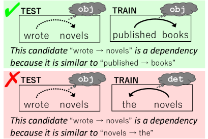
Figure 1: Valid (✔) and invalid (✗) examples of unlabeled edges for the identical subclass test.

It is an open question how to evaluate the “plausibility” of explanations: i.e., whether or not the retrieved instances as explanations are convincing for humans. As a reasonable compromise, Hanawa et al. (2021) designed the identical subclass test for evaluating the plausibility. This test is based on a minimal requirement that interpretable models should at least satisfy: training instances to be presented as explanations should belong to the same latent (sub)class as the test instance. Consider the examples in Figure 1. The predicted unlabeled edge “wrote $\rightarrow$ novels” in the test sentence has the (unobserved) latent label, obj. To this edge, two training instances are given as explanations: the above one seems more convincing than the below one because “published $\rightarrow$ books” has the same latent label, obj, as that of “wrote $\rightarrow$ novels” while “novels $\rightarrow$ the” has the different one, det. As these show, the agreement between the latent classes are likely to correlate with plausibility. Note that this test is not perfect for the plausibility assessment, but it works as a sanity check for verifying whether models make obvious violations in terms of plausibility.

This test can be used for assessing unlabeled parsing models because the (unobserved) relation labels can be regarded as the latent subclasses of positive unlabeled edges. We follow three steps; (i) identifying unlabeled edges in a development set; (ii) retrieving the nearest training edge for each identified edge; (iii) calculating LAS, i.e., if the labels of the query and retrieved edges are identical, we regard them as correct.

	Weight-Based		Instance-Based
	$\mathrm{dot}$	$\cos$	$\mathrm{dot}$	$\cos$
System ID	WId	WIc	IId	IIc
PTB-English	1.8	67.5	7.0	71.6
UD-English	16.4	51.5	3.9	54.0

Table 6: Results of the identical subclass test. Each cell indicates labeled attachment scores (LAS) on each development set. All the models are trained with head selection supervision and without labeling supervision.

Table 6 shows LAS on PTB and UD-English. The systems using instance-based inference with the cosine similarity, WIc and IIc, succeeded in retrieving the support training edges with the same label as the queries. Surprisingly, the system IIc achieved over 70% LAS on PTB without label supervision. The results suggest that systems using instance-based inference with the cosine similarity meet the minimal requirement, and the retrieved edges are promising as plausible explanations.

Query	Support
[text only label, label style=above, edge style=green!60!black,very thick] If & you & are & unsure & …
[edge unit distance=0.11cm]41	[text only label, label style=above, edge style=green!60!black,very thick] If & you & feel & this & …
[edge unit distance=0.15cm]31
[text only label, label style=above, edge style=green!60!black,very thick] … & your & appeal & is & …
[edge unit distance=0.3cm]32	[text only label, label style=above, edge style=green!60!black,very thick] … & The & food & was & …
[edge unit distance=0.3cm]32

Table 7: Examples of support edges retrieved by the instance-based system using the cosine similarity (IIc). The first query-support pair has the same (unobserved) label mark. The query of the second pair has nmod:poss although the support has det.

To facilitate the intuitive understanding of model behaviors, we show actual examples of the retrieved support edges in Table 6.2. As the first query-support pair shows, for query edges whose head or dependent is a function word (e.g., if), the training edges with the same (unobserved) label tend to be retrieved. On the other hand, as the second pair shows, for queries whose head is a noun (e.g., appeal), the edges whose head is also a noun (e.g., food) tend to be retrieved regardless of different latent labels.

6.3 Geometric Analysis on Feature Spaces

The identical subclass test suggests a big difference between the feature spaces learned by using the dot product and the cosine similarity. Here we look into them in more detail.

6.3.1 Observation of Nearest Neighbors

Query	Support
[text only label, label style=above, edge style=green!60!black,very thick] Jennifer & M. & Anderson & …
[edge unit distance=0.15cm]13	[text only label, label style=above, edge style=green!60!black,very thick] ROOT & Please & find & …
[edge unit distance=0.15cm]13
[text only label, label style=above, edge style=green!60!black,very thick] …, & after & all & …
[edge unit distance=0.3cm]32	[text only label, label style=above, edge style=green!60!black,very thick] ROOT & Please & find & …
[edge unit distance=0.15cm]13

Table 8: Examples of unlabeled support training edges retrieved by the WId system (weight-based learning and instance-based inference with the dot product) for each query. Regardless of the very different queries, the same support edge was retrieved.

First, we look into training edges retrieved as nearest support ones. Specifically, we use the edges in the UD-English development set as queries and retrieve the top $k$ similar support edges in the UD-English training set. Table 6.3.1 shows the examples retrieved by the WId system. Here, the same support edge, $\langle$ROOT, find$\rangle$, was retrieved for the different queries, $\langle$Jennifer, Anderson$\rangle$ and $\langle$all, after$\rangle$. As this indicates, when using the dot product as the similarity function, a small number of specific edges are extremely often selected as support ones for any queries. Such edges are called hubs Radovanovic et al. (2010). This phenomenon is not desirable for users in terms of the plausible interpretation of predictions. If a system always exhibits the same training instance(s) as rationales for predictions, users are likely to doubt the system’s validity.

6.3.2 Quantitative Measurement of Hubness

System ID	$\mathrm{sim}$	$N_{10}$	Instances
WId	dot	19,407	$\langle$ROOT, find$\rangle$
WIc	cos	82	$\langle$help, time$\rangle$
IId	dot	22,493	$\langle$said, airlifted$\rangle$
IIc	cos	34	$\langle$force, Israel$\rangle$

Table 9: Examples of the highest $N_{10}$ unlabeled support training edges in UD-English.

Second, we quantitatively measure the hubness of each system. Specifically, for the hubness, we measure the $k$-occurrences of instance $x$, $N_{k}(x)$ Radovanovic et al. (2010); Schnitzer et al. (2012). In the case of our dependency parsing experiments, $N_{k}(x)$ indicates the number of times each support training edge $x$ occurs among the $k$ nearest neighbors of all the query edges. The support training edges with an extremely high $N_{k}$ value can be regarded as hubs. In this study, we set $k=10$ and measure $N_{10}(x)$ of unlabeled support training edges. For query edges, we use the UD-English development set that contains $25,148$ edges. For support edges, we use the UD-English training set that contains $204,585$ edges.

Table 9 shows the highest $N_{10}$ support training edges. In the case of the system WId, the unlabeled support edge $\langle$ROOT, find$\rangle$ appeared $19,407$ times in the $10$ nearest neighbors of the $25,148$ query edges. A similar tendency was observed in the instance-based system using the dot product IId. By contrast, in the case of the systems using the cosine similarity, WIc and IIc, it was not observed that specific support edges were retrieved so often. In Figure 2, we plot the top $100$ support training edges in terms of $N_{10}$ with $\log_{10}$ scale. The $N_{10}$ distributions of the systems using the dot product, WId and IId, look very skew; that is, hubs emerge. This indicates that when using the dot product, a small number of specific support training edges appear in the nearest neighbors so often, regardless of query edges.

Figure 2: Ranking of the 100 highest $N_{10}$ unlabeled support training edges in UD-English.

To sum up, systems using instance-based inference and the dot product are often in trouble with hubs and have difficulty retrieving plausible support edges for predictions. The occurrence of hubs are likely to be related to the norms of edge representations since L2-normalization for the edges in the cosine similarity tends to suppress hubs’ occurrence. We leave a more detailed analysis of the cause of hubs’ occurrence for future work.

7 Conclusion

We have developed instance-based neural dependency parsing systems, each of which consists of our edge identification model and our label classification model (Section 4). We have analyzed them from the perspectives of the prediction accuracy and the explanation plausibility. The first analysis shows that our instance-based systems and achieve competitive accuracy with weight-based neural ones (Section 6.1). The second indicates that our instance-based systems using the cosine similarity (L2-normalization for edge representations) meet the minimal requirement of plausible explanations (Section 6.2). The additional analysis reveals that when using the dot product, hubs emerge, which degrades the plausibility (Section 6.3). One interesting future direction is investigating the cause of hubs’ occurrence in more detail. Another direction is using the learned edge representations in downstream tasks, such as semantic textual similarity.

Acknowledgments

The authors are grateful to the anonymous reviewers and the Action Editor who provided many insightful comments that improve the paper. Special thanks also go to the members of Tohoku NLP Laboratory for the interesting comments and energetic discussions. The work of H.Ouchi was supported by JSPS KAKENHI Grant Number 19K20351. The work of J.Suzuki was supported by JST Moonshot R&D Grant Number JPMJMS2011 (fundamental research) and JSPS KAKENHI Grant Number 19H04162. The work of S.Yokoi was supported by JST ACT-X Grant Number JPMJAX200S, Japan. The work of T.Kuribayashi was supported by JSPS KAKENHI Grant Number 20J22697. The work of M.Yoshikawa was supported by JSPS KAKENHI Grant Number 20K23314. The work of K.Inui was supported by JST CREST Grant Number JPMJCR20D2, Japan.

References

- Aha et al. (1991) David W Aha, Dennis Kibler, and Marc K Albert. 1991. Instance-based learning algorithms. Machine learning, 6(1):37–66.
- Akbik and Li (2016) Alan Akbik and Yunyao Li. 2016. K-SRL: Instance-based learning for semantic role labeling. In Proceedings of COLING, pages 599–608.
- Baehrens et al. (2010) David Baehrens, Timon Schroeter, Stefan Harmeling, Motoaki Kawanabe, Katja Hansen, and Klaus-Robert MÞller. 2010. How to explain individual classification decisions. Journal of Machine Learning Research, 11(Jun):1803–1831.
- Bellet et al. (2013) Aurélien Bellet, Amaury Habrard, and Marc Sebban. 2013. A survey on metric learning for feature vectors and structured data. arXiv preprint arXiv:1306.6709.
- Bod (2009) Rens Bod. 2009. From exemplar to grammar: A probabilistic analogy-based model of language learning. Cognitive Science, 33(5):752–793.
- Bordes et al. (2013) Antoine Bordes, Nicolas Usunier, Alberto Garcia-Duran, Jason Weston, and Oksana Yakhnenko. 2013. Translating embeddings for modeling multi-relational data. Proceedings of NIPS, 26:2787–2795.
- Caruana et al. (1999) Rich Caruana, Hooshang Kangarloo, John David Dionisio, Usha Sinha, and David Johnson. 1999. Case-based explanation of non-case-based learning methods. In Proceedings of the AMIA Symposium, page 212.
- Clark et al. (2018) Kevin Clark, Minh-Thang Luong, Christopher D. Manning, and Quoc Le. 2018. Semi-supervised sequence modeling with cross-view training. In Proceedings of EMNLP, pages 1914–1925.
- Daelemans and Van den Bosch (2005) Walter Daelemans and Antal Van den Bosch. 2005. Memory-based language processing. Cambridge University Press.
- Daelemans et al. (1999) Walter Daelemans, Sabine Buchholz, and Jorn Veenstra. 1999. Memory-based shallow parsing. In EACL 1999: CoNLL-99 Computational Natural Language Learning.
- Daelemans et al. (1996) Walter Daelemans, Jakub Zavrel, Peter Berck, and Steven Gillis. 1996. MBT: A memory-based part of speech tagger-generator. In Proceedings of Fourth Workshop on Very Large Corpora.
- De Meulder and Daelemans (2003) Fien De Meulder and Walter Daelemans. 2003. Memory-based named entity recognition using unannotated data. In Proceedings of HLT-NAACL, pages 208–211.
- Deng et al. (2019) Jiankang Deng, Jia Guo, Niannan Xue, and Stefanos Zafeiriou. 2019. Arcface: Additive angular margin loss for deep face recognition. In Proceedings of CVPR, pages 4690–4699.
- Devlin et al. (2019) Jacob Devlin, Ming-Wei Chang, Kenton Lee, and Kristina Toutanova. 2019. BERT: Pre-training of deep bidirectional transformers for language understanding. In Proceedings of NAACL-HLT, pages 4171–4186.
- Dozat and Manning (2017) Timothy Dozat and Christopher D Manning. 2017. Deep biaffine attention for neural dependency parsing. In Proceedings of ICLR.
- Friedman et al. (1994) Jerome H Friedman et al. 1994. Flexible metric nearest neighbor classification. Technical report.
- Goldberger et al. (2005) Jacob Goldberger, Geoffrey E Hinton, Sam T Roweis, and Ruslan R Salakhutdinov. 2005. Neighbourhood components analysis. In Proceedings of NIPS, pages 513–520.
- Grave et al. (2018) Edouard Grave, Piotr Bojanowski, Prakhar Gupta, Armand Joulin, and Tomas Mikolov. 2018. Learning word vectors for 157 languages. In Proceedings of LREC.
- Graves et al. (2013) Alan Graves, Navdeep Jaitly, and Abdel-rahman Mohamed. 2013. Hybrid speech recognition with deep bidirectional LSTM. In Proceedings of Automatic Speech Recognition and Understanding (ASRU), 2013 IEEE Workshop.
- Guu et al. (2020) Kelvin Guu, Kenton Lee, Zora Tung, Panupong Pasupat, and Ming-Wei Chang. 2020. Realm: Retrieval-augmented language model pre-training. arXiv preprint arXiv:2002.08909.
- Hadsell et al. (2006) Raia Hadsell, Sumit Chopra, and Yann LeCun. 2006. Dimensionality reduction by learning an invariant mapping. In Proceedings of CVPR, volume 2, pages 1735–1742. IEEE.
- Hanawa et al. (2021) Kazuaki Hanawa, Sho Yokoi, Satoshi Hara, and Kentaro Inui. 2021. Evaluation of similarity-based explanations. In Proceedings of ICLR.
- Hashimoto et al. (2017) Kazuma Hashimoto, Caiming Xiong, Yoshimasa Tsuruoka, and Richard Socher. 2017. A joint many-task model: Growing a neural network for multiple NLP tasks. In Proceedings of EMNLP, pages 1923–1933.
- Haspelmath et al. (2005) Martin Haspelmath, Matthew S Dryer, David Gil, and Bernard Comrie. 2005. The world atlas of language structures.
- Hastie and Tibshirani (1996) Trevor Hastie and Robert Tibshirani. 1996. Discriminant adaptive nearest neighbor classification and regression. In Proceedings of NIPS, pages 409–415.
- Hendrickx and van den Bosch (2003) Iris Hendrickx and Antal van den Bosch. 2003. Memory-based one-step named-entity recognition: Effects of seed list features, classifier stacking, and unannotated data. In Proceedings of CoNLL, pages 176–179.
- Hoffer and Ailon (2015) Elad Hoffer and Nir Ailon. 2015. Deep metric learning using triplet network. In International Workshop on Similarity-Based Pattern Recognition, pages 84–92. Springer.
- Ji et al. (2019) Tao Ji, Yuanbin Wu, and Man Lan. 2019. Graph-based dependency parsing with graph neural networks. In Proceedings of ACL, pages 2475–2485.
- Khandelwal et al. (2020) Urvashi Khandelwal, Angela Fan, Dan Jurafsky, Luke Zettlemoyer, and Mike Lewis. 2020. Nearest neighbor machine translation. arXiv preprint arXiv:2010.00710.
- Khandelwal et al. (2019) Urvashi Khandelwal, Omer Levy, Dan Jurafsky, Luke Zettlemoyer, and Mike Lewis. 2019. Generalization through memorization: Nearest neighbor language models. In Proceedings of ICLR.
- Kingma and Ba (2014) D.P. Kingma and J. Ba. 2014. Adam: A method for stochastic optimization. arXiv preprint arXiv:1412.6980.
- Kolodneer (1991) Janet L Kolodneer. 1991. Improving human decision making through case-based decision aiding. AI magazine, 12(2):52–52.
- Kübler (2004) Sandra Kübler. 2004. Memory-based parsing, volume 7.
- Kübler et al. (2009) Sandra Kübler, Ryan McDonald, and Joakim Nivre. 2009. Dependency parsing. Synthesis lectures on human language technologies, 1(1):1–127.
- Kulmizev et al. (2019) Artur Kulmizev, Miryam de Lhoneux, Johannes Gontrum, Elena Fano, and Joakim Nivre. 2019. Deep contextualized word embeddings in transition-based and graph-based dependency parsing-a tale of two parsers revisited. In Proceedings of EMNLP-IJCNLP, pages 2755–2768.
- Lebowitz (1983) Michael Lebowitz. 1983. Memory-based parsing. Artificial Intelligence, 21(4):363–404.
- Lei et al. (2016) Tao Lei, Regina Barzilay, and Tommi Jaakkola. 2016. Rationalizing neural predictions. In Proceedings of EMNLP, pages 107–117.
- Lewis et al. (2020) Patrick Lewis, Ethan Perez, Aleksandara Piktus, Fabio Petroni, Vladimir Karpukhin, Naman Goyal, Heinrich Küttler, Mike Lewis, Wen-tau Yih, Tim Rocktäschel, et al. 2020. Retrieval-augmented generation for knowledge-intensive nlp tasks. arXiv preprint arXiv:2005.11401.
- de Lhoneux et al. (2017) Miryam de Lhoneux, Sara Stymne, and Joakim Nivre. 2017. Old school vs. new school: Comparing transition-based parsers with and without neural network enhancement. In The 15th Treebanks and Linguistic Theories Workshop (TLT), pages 99–110.
- Liu et al. (2017) Weiyang Liu, Yandong Wen, Zhiding Yu, Ming Li, Bhiksha Raj, and Le Song. 2017. Sphereface: Deep hypersphere embedding for face recognition. In Proceedings of CVPR, pages 212–220.
- Marcus et al. (1993) Mitchell P. Marcus, Beatrice Santorini, and Mary Ann Marcinkiewicz. 1993. Building a large annotated corpus of English: The Penn Treebank. Computational Linguistics, 19(2):313–330.
- McDonald et al. (2006) Ryan McDonald, Kevin Lerman, and Fernando Pereira. 2006. Multilingual dependency analysis with a two-stage discriminative parser. In Proceedings of CoNLL-X, pages 216–220.
- McDonald et al. (2013) Ryan McDonald, Joakim Nivre, Yvonne Quirmbach-Brundage, Yoav Goldberg, Dipanjan Das, Kuzman Ganchev, Keith Hall, Slav Petrov, Hao Zhang, Oscar Täckström, Claudia Bedini, Núria Bertomeu Castelló, and Jungmee Lee. 2013. Universal Dependency annotation for multilingual parsing. In Proceedings of ACL, pages 92–97.
- McDonald et al. (2005) Ryan McDonald, Fernando Pereira, Kiril Ribarov, and Jan Hajič. 2005. Non-projective dependency parsing using spanning tree algorithms. In Proceedings of HLT-EMNLP, pages 523–530.
- Nagao (1984) Makoto Nagao. 1984. A framework of a mechanical translation between Japanese and English by analogy principle.
- Nickel et al. (2016) Maximilian Nickel, Lorenzo Rosasco, and Tomaso Poggio. 2016. Holographic embeddings of knowledge graphs. In Proceedings of AAAI, volume 30.
- Nivre (2003) Joakim Nivre. 2003. An efficient algorithm for projective dependency parsing. In Proceedings of the eighth international conference on parsing technologies, pages 149–160.
- Nivre et al. (2004) Joakim Nivre, Johan Hall, and Jens Nilsson. 2004. Memory-based dependency parsing. In Proceedings of CoNLL, pages 49–56.
- Oord et al. (2018) Aaron van den Oord, Yazhe Li, and Oriol Vinyals. 2018. Representation learning with contrastive predictive coding. arXiv preprint arXiv:1807.03748.
- Ouchi et al. (2020) Hiroki Ouchi, Jun Suzuki, Sosuke Kobayashi, Sho Yokoi, Tatsuki Kuribayashi, Ryuto Konno, and Kentaro Inui. 2020. Instance-based learning of span representations: A case study through named entity recognition. In Proceedings of ACL, pages 6452–6459.
- Papernot and McDaniel (2018) Nicolas Papernot and Patrick McDaniel. 2018. Deep k-nearest neighbors: Towards confident, interpretable and robust deep learning. arXiv preprint arXiv:1803.04765.
- Pascanu et al. (2013) Razvan Pascanu, Tomas Mikolov, and Yoshua Bengio. 2013. On the difficulty of training recurrent neural networks. In Proceedings of ICML, pages 1310–1318.
- Pennington et al. (2014) Jeffrey Pennington, Richard Socher, and Christopher Manning. 2014. Glove: Global vectors for word representation. In Proceedings of EMNLP, pages 1532–1543.
- Plumb et al. (2018) Gregory Plumb, Denali Molitor, and Ameet S Talwalkar. 2018. Model agnostic supervised local explanations. In Proceedings of NIPS, pages 2515–2524.
- Radovanovic et al. (2010) Milos Radovanovic, Alexandros Nanopoulos, and Mirjana Ivanovic. 2010. Hubs in space: Popular nearest neighbors in high-dimensional data. Journal of Machine Learning Research, 11(sept):2487–2531.
- Ranjan et al. (2017) Rajeev Ranjan, Carlos D Castillo, and Rama Chellappa. 2017. L2-constrained softmax loss for discriminative face verification. arXiv preprint arXiv:1703.09507.
- Ribeiro et al. (2016) Marco Tulio Ribeiro, Sameer Singh, and Carlos Guestrin. 2016. Why should i trust you?: Explaining the predictions of any classifier. In Proceedings of KDD, pages 1135–1144.
- Sang (2002) Erik F Tjong Kim Sang. 2002. Memory-based shallow parsing. Journal of Machine Learning Research, 2:559–594.
- Scha et al. (1999) Remko Scha, Rens Bod, and Khalil Sima’An. 1999. A memory-based model of syntactic analysis: data-oriented parsing. Journal of Experimental & Theoretical Artificial Intelligence, 11(3):409–440.
- Schnitzer et al. (2012) Dominik Schnitzer, Arthur Flexer, Markus Schedl, and Gerhard Widmer. 2012. Local and global scaling reduce hubs in space. Journal of Machine Learning Research, 13(10).
- Short and Fukunaga (1981) R Short and Keinosuke Fukunaga. 1981. The optimal distance measure for nearest neighbor classification. IEEE transactions on Information Theory, 27(5):622–627.
- Smith et al. (2018) Aaron Smith, Miryam de Lhoneux, Sara Stymne, and Joakim Nivre. 2018. An investigation of the interactions between pre-trained word embeddings, character models and pos tags in dependency parsing. In Proceedings of EMNLP, pages 2711–2720.
- Sohn (2016) Kihyuk Sohn. 2016. Improved deep metric learning with multi-class n-pair loss objective. In Proceedings of NIPS, pages 1857–1865.
- Sumita and Iida (1991) Eiichiro Sumita and Hitoshi Iida. 1991. Experiments and prospects of example-based machine translation. In Proceedings of ACL, pages 185–192.
- Sun et al. (2020) Yifan Sun, Changmao Cheng, Yuhan Zhang, Chi Zhang, Liang Zheng, Zhongdao Wang, and Yichen Wei. 2020. Circle loss: A unified perspective of pair similarity optimization. In Proceedings of CVPR, pages 6398–6407.
- Tjong Kim Sang (2002) Erik F. Tjong Kim Sang. 2002. Memory-based named entity recognition. In Proceedings of CoNLL.
- Veenstra et al. (2000) Jorn Veenstra, Antal Van den Bosch, Sabine Buchholz, Walter Daelemans, et al. 2000. Memory-based word sense disambiguation. Computers and the Humanities, 34(1):171–177.
- Wang et al. (2018) Hao Wang, Yitong Wang, Zheng Zhou, Xing Ji, Dihong Gong, Jingchao Zhou, Zhifeng Li, and Wei Liu. 2018. Cosface: Large margin cosine loss for deep face recognition. In Proceedings of CVPR, pages 5265–5274.
- Wang et al. (2014) Jiang Wang, Yang Song, Thomas Leung, Chuck Rosenberg, Jingbin Wang, James Philbin, Bo Chen, and Ying Wu. 2014. Learning fine-grained image similarity with deep ranking. In Proceedings of CVPR, pages 1386–1393.
- Wang et al. (2019) Xun Wang, Xintong Han, Weilin Huang, Dengke Dong, and Matthew R Scott. 2019. Multi-similarity loss with general pair weighting for deep metric learning. In Proceedings of CVPR, pages 5022–5030.