Safety-Critical Control Synthesis for Unknown Sampled-Data Systems via Control Barrier Functions

Abstract

As the complexity of control systems increases, safety becomes an increasingly important property since safety violations can damage the plant and put the system operator in danger. When the system dynamics are unknown, safety-critical synthesis becomes more challenging. Additionally, modern systems are controlled digitally and hence behave as sampled-data systems, i.e., the system dynamics evolve continuously while the control input is applied at discrete time steps. In this paper, we study the problem of control synthesis for safety-critical sampled-data systems with unknown dynamics. We overcome the challenges introduced by sampled-data implementation and unknown dynamics by constructing a set of control barrier function (CBF)-based constraints. By satisfying the constructed CBF constraint at each sampling time, we guarantee the unknown sampled-data system is safe for all time. We formulate a non-convex program to solve for the control signal at each sampling time. We decompose the non-convex program into two convex sub-problems. We illustrate the proposed approach using a numerical case study.

I Introduction

Safety-critical cyber-physical systems (CPSs) are found in applications such as autonomous vehicles and advanced manufacturing. The safety property is typically formulated as forward invariance of a given safe set. Safety violations could lead to severe damage to the controlled plant or danger to human operators [1]. Control synthesis for safety-critical CPSs has been extensively studied in existing literature when the models of the CPSs are known [2, 3, 4].

Several factors may cause safety violations of the plant even when the nominal controller is designed to be safe. One challenge is raised by the digital/discrete implementation of a continuous-time system with continuous input. In a practical digital implementation, the system state is only observable at each sampling time, and the control signal is applied in a zero-order hold (ZOH) manner during each sampling period. That is, the system is implemented as a sampled-data system. Another challenge is that the system models used to design controllers are not perfect in practice, and thus there exist uncertainties in the system model. Due to these uncertainties, the designed controller may fail to guarantee safety even if safety is guaranteed for the nominal plant.

These two challenges have been studied separately. Safety-critical control synthesis has been studied for sampled-data system with known dynamics [5, 6, 7]. For unmodeled systems with continuous-time or discrete-time dynamics, safety-critical control synthesis has been studied by assuming the existence of a backup controller that ensures safety of the unknown system [8, 9, 10], or a well-calibrated model, e.g., a model learned using a Gaussian process [11, 12, 13]. Although high-probability safety guarantees can be achieved by the methods described in [11, 12, 13], they suffer from a tradeoff between overly conservative learned model when faced with large uncertainty and the potential safety violation when failing to capture the true dynamics. To the best of our knowledge, jointly addressing these two challenges without prior knowledge of a safe backup controller or a well-calibrated model has not been studied.

In this paper, we study safety-critical control synthesis for a sampled-data system with unknown dynamics. We address the challenges introduced due to the sampled-data system and unknown dynamics by developing a set control barrier function (CBF) constraints at each sampling time. A CBF constraint is an inequality that is imposed on the control signal, whose satisfaction implies forward invariance. We estimate the constructed CBF constraints by bounding the reachable set during each sampling period and calculating an interval that contains the system dynamics, leveraging the Lipschitz continuity assumption on the system dynamics. By satisfying these CBF constraints at each sampling time, the system is guaranteed to be safe for all time. To summarize, this paper makes the following contributions.

• We construct a CBF constraint for the unknown sampled-data system. We provide a sufficient condition for satisfying the CBF constraint by bounding the set of reachable states for each sampling period and calculating an interval which contains the unknown system dynamics.

• We formulate a non-convex optimization problem subject to the constructed CBF constraints to calculate the ZOH control signal for each sampling period. We solve the non-convex optimization problem by proposing a two-stage approach which only involves convex programs.

• We prove that the synthesized controller ensures the system is safe with respect to the given safe set.

• We validate our proposed framework using a numerical case study on a DC motor. We show that our proposed approach ensures the safety of the DC motor.

The remainder of this paper is organized as follows. We review the related work and preliminary background in Section II and Section III, respectively. The system model and problem formulation are presented in Section IV. We give the solution approach in Section V, and illustrate the proposed approach using a numerical case study in Section VI. Section VII concludes this paper.

II Related Work

Multiple approaches have been proposed for safety-critical control synthesis for CPSs with known dynamics, including Hamilton-Jacobi-Bellman-Isaacs (HJI) equation [14], mixed-integer program [15], and control barrier function (CBF) and control Lyapunov function (CLF) -based methodologies [2, 3, 4]. The CBF-based methods formulate a quadratic program to calculate the controller, assuming the system state remains unchanged during the discrete time interval.

For sampled-data systems, CBF-based approaches have shown great success [5, 6, 7]. The authors of [5] and [7] focus on sampled-data systems with known dynamics. In [6], a sampled-data system with an additive disturbance is studied. In this work, we consider a sampled-data system with unknown dynamics. CBF-based methods normally require the knowledge of the system dynamics to calculate the CBF constraint. The unknown dynamics lead to a scenario where calculating the CBF constraints is not feasible, and thus makes the approaches proposed in [5, 6, 7] not applicable.

Learning-based control algorithms have been proposed to address systems that contain unknown uncertainties. Recent works have demonstrated the success of CBF- and/or CLF- based method along with learning algorithms [11, 16, 17, 10]. This category of approaches leverages the forward invariance and stability properties provided by barrier functions and Lyapunov functions, respectively. However, they assume that there exists a well-calibrated model of the unknown system [13] and a safe backup controller to recover from failure [8]. Moreover, CBF-based learning approaches have to handle the tradeoff between the overly constrained learned model and failure to capture the true dynamics.

Reachable set learning aims at learning the set of reachable states of the system so as to compute a controller that gives no intersection between the reachable states and the unsafe region [18]. The computation of reachable sets relies on numerically solving HJI equations, which incurs high computational complexity and poor scalability [19, 20]. A Gaussian Process based reachability analysis is proposed in [21] to compute the reachable set. Compared with forward reachable set computation, region-of-attraction focuses on computing the set of states starting from which the system is guaranteed to be safe [13]. These learning-based approaches focus on either continuous-time or discrete-time systems. In this work, we study safety-critical control synthesis for the unknown sampled-data system.

III Preliminary Background

III-A Control Barrier Function

A continuous function $\alpha:[0,a)\mapsto[0,\infty)$ belongs to class $\mathcal{K}$ if it is strictly increasing and $\alpha(0)=0$. A continuous function $\alpha:[-b,a)\mapsto(-\infty,\infty)$ is said to belong to extended class $\mathcal{K}$ if it is strictly increasing and $\alpha(0)=0$ for some $a,b>0$.

Consider a continuous-time control-affine system

$$\dot{x}_{t}=f(x_{t})+g(x_{t})u_{t}$$ (1)

where $x_{t}\in\mathcal{X}\subseteq\mathbb{R}^{n}$ is the system state and $u_{t}\in\mathcal{U}\subseteq\mathbb{R}^{m}$ is input provided by the controller. Vector-valued and matrix-valued functions $f(x_{t})$ and $g(x_{t})$ are of appropriate dimensions. Let a safe set $\mathcal{C}$ be defined as

$$\mathcal{C}=\{x\in\mathcal{X}:h(x)\geq 0\},$$ (2)

where $h:\mathcal{X}\mapsto\mathbb{R}$ is a continuously differentiable function. We say system (1) is safe with respect to $\mathcal{C}$ if $x_{t}\in\mathcal{C}$ for all time $t\geq 0$.

CBF-based approaches have been used to guarantee safety of system (1) with respect to safe set $\mathcal{C}$. We give the definition of zeroing CBF as follows.

Definition 1 (Zeroing CBF (ZCBF) [2]).

Consider a dynamical system (1) and a continuously differentiable function $h:\mathcal{X}\mapsto\mathbb{R}$. If there exists a locally Lipschitz extended class $\mathcal{K}$ function $\alpha$ such that for all $x\in\mathcal{X}$ the following inequality holds

$$\sup_{u\in\mathcal{U}}\bigg{\{}\frac{\partial h(x)}{\partial x}f(x)+\frac{\partial h(x)}{\partial x}g(x)u+\alpha(h(x))\bigg{\}}\geq 0,$$

then function $h$ is a ZCBF.

In this paper, we focus on ZCBF. Extensions to higher relative degree CBFs are subject to our future work. A sufficient condition for the safety guarantee can be derived using ZCBF as follows.

Lemma 1 ([2]).

Given a dynamical system (1) and a safe set (2) defined by some continuously differentiable function $h:\mathcal{X}\mapsto\mathbb{R}$, if $h$ is a ZCBF defined on $\mathcal{X}$, then $\mathcal{C}$ is forward invariant.

Using Lemma 1, one can solve for the controller at each time using a quadratic program [2]

$$\min_{u}~{} u^{\top}R(x)u+Q(x)^{\top}u$$ (3a)

s.t. $$\frac{\partial h(x)}{\partial x}f(x)+\frac{\partial h(x)}{\partial x}g(x)u+\alpha(h(x))\geq 0$$ (3b)

$$u\in\mathcal{U}$$ (3c)

where $R(x)\in\mathbb{R}^{m}$ is positive definite and $Q(x)\in\mathbb{R}^{m}$.

III-B Notations

Let $x$ be a vector and $f(x)$ be a vector-valued function, we use $x_{j}$ and $f_{j}(x)$ to denote their $j$-th component, respectively. Let $A$ be a matrix. We use $A_{i,j}$ to denote its element at $i$-th row and $j$-th column. Let $x_{t}$ be a vector at time $t$. We use $x_{t,j}$ to denote the $j$-th component of $x_{t}$. Comparisons between vectors are implemented element-wise. Bold symbols are used to represent intervals.

IV Problem Formulation

Consider a continuous-time control-affine system in the form of (1). The system contains uncertainties and hence $f(x_{t})$ and $g(x_{t})$ are unknown. We define a feedback controller $\mu:\mathcal{X}\mapsto\mathcal{U}$ to be a function that maps the system state to a control input. Given the current system state $x_{t}$ at time $t$ and a feedback controller $\mu$, we denote the system state at time $t^{\prime}$ as $\varphi^{t^{\prime}}(x_{t},\mu)$. The system is given a safe set as defined in (2).

We consider the sampled-data implementation of system (1). That is, the system is sampled using a sampling period $\Delta t$. Only the system states $x_{z\Delta t}$ at the sampling time are known, where $z=0,1,\ldots$. At each sampling time, a zero-order hold (ZOH) feedback controller $\mu(x_{z\Delta t})$ is applied to system (1). In other words, $u_{t}=\mu(x_{z\Delta t})$ for all $t\in[z\Delta t,(z+1)\Delta t)$.

We have a data set of system (1) as side information. Let $K\in\mathbb{N}$ and $K\geq 1$. We denote a finite set of $K$ samples of state-input pairs as $R_{K}=\{(x_{t_{k}},u_{t_{k}},x_{t_{k+1}})\}_{k=1}^{K}$ where $x_{t_{k+1}}=\varphi^{t_{k+1}}(x_{t_{k}},\mu)$. Here $\mu$ represents a zero-order hold (ZOH) input $u_{t}=u_{t_{k}}$ for all time $t\in[t_{k},t_{k+1})$. We assume that $h(x_{t_{k}})\geq 0$ for all $k=1,\ldots,K$.

In the following, we formally state our assumptions.

Assumption 1.

We assume that functions $f_{j}(x)$ and $g_{j,s}(x)$ are Lipschitz continuous with Lipschitz constants $L_{f_{j}}$ and $L_{g_{j,s}}$, respectively, for all $j=1,\ldots,n$ and $s=1,\ldots,m$. The Lipschitz constants are known. We assume that $\sup_{x\in\mathcal{C}}\|f(x)\|$ and $\sup_{x\in\mathcal{C}}\|g(x)\|$ are given.

Lipschitz continuity is a commonly made assumption for reachability and safety analysis [10, 3, 22]. The assumption on the bound of system dynamics is often seen in the worst-case safety analysis [18, 13].

Assumption 2.

We assume that the safe set $\mathcal{C}$ and control input set $\mathcal{U}$ are compact. Additionally, control input set $\mathcal{U}$ is convex.

The problem studied in this work is as follows.

Problem 1.

Given a finite set of samples $R_{K}=\{(x_{t_{k}},u_{t_{k}})\}_{k=1}^{K}$ for some $K\in\mathbb{N}$ generated by implementing a given control input $u_{t_{k}}$ for all time $t\in[t_{k},t_{k+1})$ to system (1) whose dynamics are unknown, synthesize a ZOH feedback controller $\mu$ such that system (1) is safe with respect to set $\mathcal{C}=\{x:h(x)\geq 0\}$.

V Solution Approach

Our solution approach leverages Lemma 1 to guarantee safety of the system. We first construct a CBF constraint for the unknown sampled-data system to ensure the safety. Then we calculate a bound for the unknown system dynamics to evaluate the constructed CBF constraint. Finally, we formulate an optimization problem to solve for the control signal at each sample time.

V-A Construction of CBF Constraints for Unknown Systems

When the system model is known and the system state is observable for all time $t\geq 0$, safety-critical synthesis can be achieved efficiently using quadratic program (3). We consider the sampled-data system with unknown dynamics, which makes it difficult to evaluate the constraint given in (3b). In this subsection, we construct a CBF constraint that can be evaluated at each sampling time for unknown sampled-data system to guarantee that (3b) holds for all time $t\in[z\Delta t,(z+1)\Delta t)$ for each sampling period $z=0,1,\ldots$, and hence guarantee system safety.

Inspired by [6], for any $t\in[z\Delta t,(z+1)\Delta t)$, we define

$$e(x_{t},x_{z\Delta t},u_{z\Delta t})=\frac{\partial h(x_{z\Delta t})}{\partial x}[f(x_{z\Delta t})+g(x_{z\Delta t})u_{z\Delta t}]\\ +\alpha(h(x_{z\Delta t}))-\frac{\partial h(x_{t})}{\partial x}[f(x_{t})-g(x_{t})u_{z\Delta t}]-\alpha(h(x_{t})).$$ (4)

The definition given in (4) models the difference between the CBF constraints evaluated at states $x_{z\Delta t}$ and $x_{t}$ when control input $u_{z\Delta t}$ is applied. Given (4), we have that

$$\frac{\partial h(x_{t})}{\partial x}f(x_{t})+\frac{\partial h(x_{t})}{\partial x}g(x_{t})u_{t}+\alpha(h(x_{t}))$$

$$= \frac{\partial h(x_{z\Delta t})}{\partial x}f(x_{z\Delta t})+\frac{\partial h(x_{z\Delta t})}{\partial x}g(x_{z\Delta t})u_{z\Delta t}$$

$$\quad\quad\quad\quad\quad\quad+\alpha(h(x_{z\Delta t}))-e(x_{t},x_{z\Delta t},u_{z\Delta t})$$ (5a)

$$\geq \frac{\partial h(x_{z\Delta t})}{\partial x}f(x_{z\Delta t})+\frac{\partial h(x_{z\Delta t})}{\partial x}g(x_{z\Delta t})u_{z\Delta t}$$

$$\quad+\alpha(h(x_{z\Delta t}))-\max_{x_{t},x_{z\Delta t},u_{z\Delta t}}|e(x_{t},x_{z\Delta t},u_{z\Delta t})|$$ (5b)

If we can guarantee that the right-hand side of (5) is non-negative, then safety of system (1) holds by Lemma 1. We define the following quantities:

$$\theta(u)=\sqrt{\sum_{j=1}^{n}\left(L_{f_{j}}+\sum_{s=1}^{m}L_{g_{j,s}}|u_{s}|\right)^{2}},\quad\Theta=\max_{u\in\mathcal{U}}\theta(u).$$ (6)

The existence of $\Theta$ is guaranteed by Assumption 2. In the following, we bound $\max_{x_{t},x_{z\Delta t},u_{z\Delta t}}|e(x_{t},x_{z\Delta t},u_{z\Delta t})|$ from above to calculate a lower bound for (5).

Lemma 2.

Let $L_{\alpha}$ and $L_{h}$ be the Lipschitz constants of functions $\alpha$ and $h$, respectively. Let $\Theta$ be defined as in (6). Then for any given $x_{z\Delta t}$, $x_{t}$, and $u_{z\Delta t}$, we have

$$|e(x_{t},x_{z\Delta t},u_{z\Delta t})|\leq(L_{h}\Theta+L_{\alpha})\|x_{z\Delta t}-x_{t}\|_{2}\\ +2L_{h}\|f(x_{z\Delta t})+g(x_{z\Delta t})u_{z\Delta t}\|_{2}.$$ (7)

Proof.

We bound $|e(x_{t},x_{z\Delta t},u_{z\Delta t})|$ via

$$|e(x_{t},x_{z\Delta t},u_{z\Delta t})|$$

$$= \Big{|}\frac{\partial h(x_{z\Delta t})}{\partial x}[f(x_{z\Delta t})+g(x_{z\Delta t})u_{z\Delta t}]+\alpha(h(x_{z\Delta t}))$$

$$-\frac{\partial h(x_{t})}{\partial x}[f(x_{t})-g(x_{t})u_{z\Delta t}]-\alpha(h(x_{t}))\Big{|}$$ (8a)

$$= \Big{|}\frac{\partial h(x_{z\Delta t})}{\partial x}[f(x_{z\Delta t})+g(x_{z\Delta t})u_{z\Delta t}]$$

$$\quad-\frac{\partial h(x_{t})}{\partial x}[f(x_{z\Delta t})+g(x_{z\Delta t})u_{z\Delta t}]+\frac{\partial h(x_{t})}{\partial x}[f(x_{z\Delta t})$$

$$\quad+g(x_{z\Delta t})u_{z\Delta t}]-\frac{\partial h(x_{t})}{\partial x}[f(x_{t})+g(x_{t})u_{z\Delta t}]$$

$$\quad\quad\quad\quad+\alpha(h(x_{z\Delta t}))-\alpha(h(x_{t}))\Big{|}$$ (8b)

$$\leq \Big{|}\left(\frac{\partial h(x_{z\Delta t})}{\partial x}-\frac{\partial h(x_{t})}{\partial x}\right)[f(x_{z\Delta t})+g(x_{z\Delta t})u_{z\Delta t}]\Big{|}$$

$$+\Big{|}\frac{\partial h(x_{t})}{\partial x}[f(x_{z\Delta t})+g(x_{z\Delta t})u_{z\Delta t}-f(x_{t})-g(x_{t})u_{z\Delta t}]\Big{|}$$

$$\quad\quad\quad\quad\quad+|\alpha(h(x_{z\Delta t}))-\alpha(h(x_{t}))|$$ (8c)

where (8a) holds by definition given in (4), (8b) holds by adding and subtracting $\frac{\partial h(x_{t})}{\partial x}[f(x_{z\Delta t})+g(x_{z\Delta t})u_{z\Delta t}]$, and (8c) holds by triangle inequality.

Since function $h$ is continuously differentiable, we have that $\|\frac{\partial h(x)}{\partial x}\|\leq L_{h}$, where $L_{h}$ is the Lipschitz constant of $h$. Hence we have that

$$\Big{|}\left(\frac{\partial h(x_{z\Delta t})}{\partial x}-\frac{\partial h(x_{t})}{\partial x}\right)[f(x_{z\Delta t})+g(x_{z\Delta t})u_{z\Delta t}]\Big{|}\\ \leq 2L_{h}\|f(x_{z\Delta t})+g(x_{z\Delta t})u_{z\Delta t}\|_{2}.$$ (9)

By the boundedness of $\frac{\partial h(x)}{\partial x}$ and Proposition 3 in the Appendix, we have that

$$\Big{|}\frac{\partial h(x_{t})}{\partial x}[f(x_{z\Delta t})+g(x_{z\Delta t})u_{z\Delta t}-f(x_{t})-g(x_{t})u_{z\Delta t}]\Big{|}\\ \leq L_{h}\Theta\|x_{z\Delta t}-x_{t}\|_{2}.$$ (10)

Due to Lipschitz continuity of $\alpha(\cdot)$, we have that

$$|\alpha(h(x_{z\Delta t}))-\alpha(h(x_{t}))|\leq L_{\alpha}\|x_{z\Delta t}-x_{t}\|_{2}.$$ (11)

Substituting (9) - (11) into (8c) yields the lemma. ∎

Using Lemma 2, we can construct a CBF constraint as

$$\frac{\partial h(x_{z\Delta t})}{\partial x}f(x_{z\Delta t})+\frac{\partial h(x_{z\Delta t})}{\partial x}g(x_{z\Delta t})u_{z\Delta t}\\ +\alpha(h(x_{z\Delta t}))-(L_{h}\Theta+L_{\alpha})\|x_{z\Delta t}-x_{t}\|_{2}\\ -2L_{h}\|f(x_{z\Delta t})+g(x_{z\Delta t})u_{z\Delta t}\|_{2}\geq 0.$$ (12)

Using (5), we have that if (12) holds, then Lemma 1 holds for all $t\in[z\Delta t,(z+1)\Delta t)$. However, since the system is unknown, we cannot compute $x_{t}$ and $\|f(x_{z\Delta t})+g(x_{z\Delta t})u_{z\Delta t}\|_{2}$, and thus we cannot calculate constraint (12). In the subsequent subsection, we address this challenge.

V-B Sufficient Condition for Satisfying CBF Constraint (12)

Since we consider sampled-data systems, only system states at time $z\Delta t$ with $z=0,1,\ldots$ are observable. Hence, $x_{t}$ in (12) is not known. Moreover, the term $\|f(x_{z\Delta t})+g(x_{z\Delta t})u_{z\Delta t}\|_{2}$ is not known since the system is unknown. In this subsection, we present how to estimate $x_{t}$ and $\|f(x_{z\Delta t})+g(x_{z\Delta t})u_{z\Delta t}\|_{2}$ to calculate the constructed CBF constraint given in (12).

V-B1 Estimate System State $x_{t}$ During Sampling Period

Although it is impractical to forward integrate the unknown dynamics to calculate $x_{t}$, we can bound $\|x_{z\Delta t}-x_{t}\|_{2}$. Using such bound and the observed system state $x_{z\Delta t}$, we can bound $x_{t}$ during each sampling period. We define

$$\beta=\sup_{x\in\mathcal{C},u\in\mathcal{U}}(\|f(x)+g(x)u\|).$$ (13)

The existence of $\beta$ is guaranteed by Assumption 2. We can now bound $\|x_{z\Delta t}-x_{t}\|_{2}$ using the following proposition.

Proposition 1.

Let $x_{t}\in\mathcal{X}$ and $\mu$ be a controller that specifies the control signal $u_{t}$ applied to system (1) for each time $t\in[T,T+\Delta t]$. We have that

$$\left\|\varphi^{t}(x_{t},\mu)-\varphi^{T}(x_{t},\mu)\right\|_{2}\leq\frac{\|\beta\|_{2}}{\Theta}(e^{\Theta\Delta t}-1),$$ (14)

where $\Theta$ is given in (6), and $\beta$ is given in (13).

Proof.

By definition of $\varphi^{t}(x,\mu)$, we have that

$$\left\|\varphi^{t}(x_{t},\mu)-\varphi^{T}(x_{t},\mu)\right\|_{2}$$

$$= \Big{\|}\int_{T}^{t}\left(f(x_{\tau})+g(x_{\tau})u_{\tau}\right)\,\textrm{d}{\tau}\Big{\|}_{2}$$ (15a)

$$\leq \Big{\|}\int_{T}^{t}\left\{f(x_{\tau})+g(x_{\tau})u_{\tau}-f(x_{T})-g(x_{T})u_{\tau}\right\}\,\textrm{d}{\tau}\Big{\|}_{2}$$

$$\quad\quad\quad\quad\quad+\left\|\int_{T}^{t}\left(f(x_{T})+g(x_{T})u_{\tau}\right)\,\textrm{d}{\tau}\right\|_{2}$$ (15b)

$$\leq \int_{T}^{t}\theta(u_{\tau})\|x_{\tau}-x_{T}\|_{2}\,\textrm{d}{\tau}+\|\beta\|_{2}(t-T).$$ (15c)

where (15a) holds by definition of $\varphi^{t}(x_{t},\mu)$, (15b) holds by triangle inequality, and (15c) holds by Proposition 3 in the Appendix and (13).

Applying Grönwall’s inequality [23] to (15) yields that

$$\left\|\varphi^{t}(x_{t},\mu)-\varphi^{T}(x_{t},\mu)\right\|_{2}$$

$$\leq \int_{T}^{t}\theta(u_{\tau})\|x_{\tau}-x_{T}\|_{2}\,\textrm{d}{\tau}+\|\beta\|_{2}(t-T)$$ (16a)

$$\leq \|\beta\|_{2}(t-T)$$

$$+\int_{T}^{t}\|\beta\|_{2}(t-T)\theta(u_{\tau})\exp{\left(\int_{\tau}^{t}\theta(u_{l})\,\textrm{d}{l}\right)}\,\textrm{d}{\tau}$$ (16b)

$$\leq \|\beta\|_{2}(t-T)+\|\beta\|_{2}\Theta\int_{T}^{t}(\tau-T)e^{\Theta(t-\tau)}\,\textrm{d}{\tau}$$ (16c)

$$\leq \frac{\|\beta\|_{2}}{\Theta}(e^{\Theta\Delta t}-1)$$ (16d)

where (16a) holds by (15), (16b) holds by Grönwall’s inequality [23], (16c) holds by (6) and calculating the inner integration, and (16d) holds by integration by parts and $t\in[T,T+\Delta t]$. ∎

Proposition 1 is closely related to [22, Thm 3.4]. In [22, Thm 3.4], an upper bound of the distance between two nonlinear systems is established for each time, while Proposition 1 presents an upper bound of the distance between reachable states during a sampling period for the sampled-data system.

By Proposition 1, we have that $\|x_{z\Delta t}-x_{t}\|_{2}\leq\frac{\|\beta\|_{2}}{\Theta}(e^{\Theta\Delta t}-1)$. For a sampled-data system, state $x_{z\Delta t}$ can be observed. Therefore, we can calculate a bound for $x_{t}$ for all $t\in[z\Delta t,(z+1)\Delta t)$ for all non-negative integer $z$.

V-B2 Estimate the Unknown System Dynamics

In the following, we calculate a bound of $\|f(x_{z\Delta t})+g(x_{z\Delta t})u_{z\Delta t}\|_{2}$ for the unknown system. We define

$$\gamma(u,u^{\prime})=\sup_{x\in\mathcal{C}}\|g(x)\|\|u-u^{\prime}\|_{2},$$ (17)

for all $u,u^{\prime}\in\mathcal{U}$, and develop the following result.

Proposition 2.

Let $x_{z\Delta t}\in\mathcal{X}$, $\Theta$ be given in (6), and $\beta$ be given in (13). We have the following relation:

$$\|f(x_{z\Delta t})+g(x_{z\Delta t})u_{z\Delta t}-f(x)-g(x)u\|_{2}\\ \leq\theta(u)\|x_{z\Delta t}-x\|_{2}+\gamma(u_{z\Delta t},u),$$ (18)

where $\gamma(u_{z\Delta t},u)$ is defined in (17).

Proof.

We have that

$$\|f(x_{z\Delta t})+g(x_{z\Delta t})u_{z\Delta t}-f(x)-g(x)u\|_{2}$$

$$= \|f(x_{z\Delta t})+g(x_{z\Delta t})u-f(x)-g(x)u$$

$$\quad\quad\quad-g(x_{z\Delta t})u+g(x_{z\Delta t})u_{z\Delta t}\|_{2}$$ (19a)

$$\leq \theta(u)\|x_{z\Delta t}-x\|_{2}+\|g(x_{z\Delta t})(u_{z\Delta t}-u_{t_{k}})\|_{2}$$ (19b)

$$\leq \theta(u)\|x_{z\Delta t}-x\|_{2}+\gamma(u_{z\Delta t},u)$$ (19c)

where (19a) holds by adding and subtracting term $g(x_{z\Delta t})u_{t_{k}}$, (19b) holds by triangle inequality and Proposition 3 in the Appendix, and (19c) holds by the fact that $\gamma(u_{z\Delta t},u_{t_{k}})\geq\|g(x_{z\Delta t})(u_{z\Delta t}-u_{t_{k}})\|_{2}$. ∎

Proposition 2 implies that once the value of $f(x)+g(x)u$ is known for some $x\in\mathcal{X}$ and $u\in\mathcal{U}$, we are able to calculate the range of $f(x_{z\Delta t})+g(x_{z\Delta t})u_{z\Delta t}$. In the following, we show how to construct $f(x)+g(x)u$ so as to bound $f(x_{z\Delta t})+g(x_{z\Delta t})u_{z\Delta t}$.

Lemma 3.

Let $x_{t_{k}},x_{t_{k+1}}\in R_{K}$ be two sample data points. We can construct a vector $\dot{x}$ entry-wise as

$$\dot{x}_{j}\doteq f_{j}(x)+(g(x)u_{t_{k}})_{j}=\frac{x_{t_{k+1},j}-x_{t_{k},j}}{t_{k+1}-t_{k}}.$$ (20)

Then the system dynamics $f(x_{z\Delta t})+g(x_{z\Delta t})u_{z\Delta t}$ satisfies

$$f(x_{z\Delta t})+g(x_{z\Delta t})u_{z\Delta t}\in\dot{\mathbf{x}}\\ +\Big{(}\theta(u_{t_{k}})\|x_{z\Delta t}-x_{t_{k}}\|_{2}+\frac{\theta(u_{t_{k}})\sqrt{n}\|\beta\|_{2}}{\Theta}\left(e^{\Theta(t_{k+1}-t_{k})}-1\right)\\ +\gamma(u_{z\Delta t},u_{t_{k}})\Big{)}[-1,1]^{n},$$ (21)

where $\dot{\mathbf{x}}=[\dot{x},\dot{x}]$ is a thin interval.

Proof.

By the mean value theorem, we have that there must exist a set of states $\{x_{\tau_{j}}\in\mathbb{R}^{n}:j=1,\ldots,n\}$ such that $\tau_{j}\in(t_{k},t_{k+1})$ for all $j$ and the $j$-th entry of $x_{\tau_{j}}$, denoted as $x_{\tau_{j},j}$, satisfies $x_{\tau_{j},j}=\frac{x_{t_{k+1},j}-x_{t_{k},j}}{t_{k+1}-t_{k}}$. Given the set of states $\{x_{\tau_{j}}\in\mathbb{R}^{n}:j=1,\ldots,n\}$, we can construct $\dot{x}$ entry-wise as $\dot{x}=[\dot{x}_{1},\ldots,\dot{x}_{n}]^{\top}$, where $\dot{x}_{j}=x_{\tau_{j},j}$ for each $j=1,\ldots,n$.

Let $\dot{x}$ be constructed as (20). We define $\dot{\mathbf{x}}=[\dot{x},\dot{x}]$. Given $\dot{\mathbf{x}}$, we then show that (21) holds as follows.

$$f(x_{z\Delta t})+g(x_{z\Delta t})u_{z\Delta t}$$

$$\in \dot{\mathbf{x}}+(\theta(u_{t_{k}})\|x_{z\Delta t}-x\|_{2}+\gamma(u_{z\Delta t},u_{t_{k}}))[-1,1]^{n}$$ (22a)

$$= \dot{\mathbf{x}}+(\theta(u_{t_{k}})\|x_{z\Delta t}+x_{t_{k}}-x_{t_{k}}-x\|_{2}$$

$$\quad\quad\quad\quad\quad\quad\quad+\gamma(u_{z\Delta t},u_{t_{k}}))[-1,1]^{n}$$ (22b)

$$\subseteq \dot{\mathbf{x}}+(\theta(u_{t_{k}})\|x_{z\Delta t}-x_{t_{k}}\|_{2}+\theta(u_{t_{k}})\|x_{t_{k}}-x\|_{2}$$

$$\quad\quad\quad\quad\quad\quad\quad+\gamma(u_{z\Delta t},u_{t_{k}}))[-1,1]^{n},$$ (22c)

where (22a) holds by Proposition 2 and the fact that the sample data is generated using ZOH control input $u_{t}=u_{t_{k}}$ for all $t\in[t_{k},t_{k+1})$, (22b) holds by adding and subtracting term $x_{t_{k}}$, and (22c) holds by triangle inequality.

We prove (21) using the following relation

$$|x_{t_{k},j}-x_{j}| =|x_{t_{k},j}-x_{\tau_{j},j}|$$

$$\leq\frac{\|\beta\|_{2}}{\Theta}\left(e^{\Theta(t_{k+1}-t_{k})}-1\right),$$

where the equality holds by (20) and the inequality holds by Proposition 1. Therefore, we can bound $\|x_{t_{k}}-x\|_{2}$ as

$$\|x_{t_{k}}-x\|_{2}\leq\frac{\sqrt{n}\|\beta\|_{2}}{\Theta}\left(e^{\Theta(t_{k+1}-t_{k})}-1\right).$$ (23)

Combining (23) with (22) yields the lemma. ∎

Proposition 1 and Lemma 3 provides us the methods to estimate the CBF constraint given in (12). In the next subsection, we present an optimization problem subject to the CBF constraint for safety-critical synthesis.

V-C Safety-Critical Synthesis

In this subsection, we first use Proposition 1 and Lemma 3 to evaluate the CBF constraint given in (12). We show that the safety-critical synthesis using the evaluated CBF constraint is formulated as a non-convex program. We decompose the non-convex program to two convex sub-problems, and present an efficient safety-critical synthesis.

We define

$$w(u_{z\Delta t},u_{t_{k}})=\theta(u_{t_{k}})\|x_{z\Delta t}-x_{t_{k}}\|_{2}\\ +\frac{\sqrt{n}\theta(u_{t_{k}})\|\beta\|_{2}}{\Theta}\left(e^{\Theta(t_{k+1}-t_{k})}-1\right)+\gamma(u_{z\Delta t},u_{t_{k}}).$$

Using Proposition 1 and Lemma 3, we have the following upper bound for $e(x_{t},x_{z\Delta t},u_{z\Delta t})$ defined in (4).

Theorem 1.

Let $\dot{x}\in\mathbb{R}^{n}$ be constructed as (20), $\mathbf{1}=[1,\ldots,1]^{\top}\in\mathbb{R}^{n}$, and

$$E(\Delta t,u_{z\Delta t})=\frac{L_{h}\Theta\|\beta\|_{2}+L_{\alpha}}{\Theta}(e^{\Theta\Delta t}-1)\\ +2L_{h}\max\{\|\dot{x}+w(u_{z\Delta t},u_{t_{k}})\mathbf{1}\|_{2},\|\dot{x}-w(u_{z\Delta t},u_{t_{k}})\mathbf{1}\|_{2}\}.$$ (24)

Then $|e(x_{t},x_{z\Delta t},u_{z\Delta t})|\leq E(\Delta t,u_{z\Delta t})$ for all $u_{z\Delta t}\in\mathcal{U}$.

Proof.

The theorem follows from Lemma 2, Proposition 1, and Lemma 3. ∎

Using Theorem 1, we have the following result.

Lemma 4.

Let $\dot{x}\in\mathbb{R}^{n}$ be constructed as (20) and $\mathbf{1}=[1,\ldots,1]^{\top}\in\mathbb{R}^{n}$. If a control signal $u\in\mathcal{U}$ satisfies the following set of relations

$$\frac{\partial h(x_{z\Delta t})}{\partial x}(\dot{x}+w(u_{z\Delta t},u_{t_{k}})\mathbf{1})+\alpha(h(x_{z\Delta t}))$$

$$\quad\quad\quad\quad\quad\quad\quad\quad\quad\quad-E(\Delta t,u_{z\Delta t})\geq 0$$ (25a)

$$\frac{\partial h(x_{z\Delta t})}{\partial x}(\dot{x}-w(u_{z\Delta t},u_{t_{k}})\mathbf{1})+\alpha(h(x_{z\Delta t}))$$

$$\quad\quad\quad\quad\quad\quad\quad\quad\quad\quad-E(\Delta t,u_{z\Delta t})\geq 0$$ (25b)

then control signal $u$ satisfies

$$\frac{\partial h(x_{z\Delta t})}{\partial x}(f(x_{z\Delta t})+g(x_{z\Delta t})u)+\alpha(h(x_{z\Delta t}))\geq 0.$$

Proof.

By Theorem 1, we have $|e(x_{t},x_{z\Delta t},u_{z\Delta t})|\leq E(\Delta t,u_{z\Delta t})$. Therefore, if (25) holds, then

$$\frac{\partial h(x_{z\Delta t})}{\partial x}(\dot{x}+w(u,u_{t_{k}})\mathbf{1})+\alpha(h(x_{z\Delta t}))$$

$$\quad\quad\quad\quad\quad\quad\quad-|e(x_{t},x_{z\Delta t},u)|\geq 0$$ (26a)

$$\frac{\partial h(x_{z\Delta t})}{\partial x}(\dot{x}-w(u,u_{t_{k}})\mathbf{1})+\alpha(h(x_{z\Delta t}))$$

$$\quad\quad\quad\quad\quad\quad\quad-|e(x_{t},x_{z\Delta t},u)|\geq 0$$ (26b)

Using Lemma 3, we have that

$$\frac{\partial h(x_{z\Delta t})}{\partial x}(f(x_{z\Delta t})+g(x_{z\Delta t})u)\\ \in\frac{\partial h(x_{z\Delta t})}{\partial x}[\dot{x}-w(u,u_{t_{k}})),\dot{x}+w(u,u_{t_{k}}))].$$ (27)

Hence, (26) implies that

$$\frac{\partial h(x_{z\Delta t})}{\partial x}(f(x_{z\Delta t})+g(x_{z\Delta t})u)+\alpha(h(x_{z\Delta t}))\\ -|e(x_{t},x_{z\Delta t},u)|\geq 0$$

Note that $|e(x_{t},x_{z\Delta t},u)|\geq 0$. Therefore, the lemma holds. ∎

Motivated by Lemma 4, we can formulate the following optimization problem at each sampling time $z\Delta t$ for all $z$

$$\min_{u}~{} u^{\top}R(x_{z\Delta t})u$$ (28a)

s.t. $$\frac{\partial h(x_{z\Delta t})}{\partial x}(\dot{x}+w(u,u_{t_{k}})\mathbf{1})+\alpha(h(x_{z\Delta t}))$$

$$\quad\quad\quad\quad\quad\quad\quad\quad\quad\quad-E(\Delta t,u)\geq 0$$ (28b)

$$\frac{\partial h(x_{z\Delta t})}{\partial x}(\dot{x}-w(u,u_{t_{k}})\mathbf{1})+\alpha(h(x_{z\Delta t}))$$

$$\quad\quad\quad\quad\quad\quad\quad\quad\quad\quad-E(\Delta t,u)\geq 0$$ (28c)

$$u\in\mathcal{U}$$ (28d)

where $R(x_{z\Delta t})\in\mathbb{R}^{m}$ is a positive definite matrix. According to (5) and Lemma 4, we have that if a control signal $u\in\mathcal{U}$ satisfying (28) at sampling time $z\Delta t$ is implemented during sampling period $[z\Delta t,(z+1)\Delta t)$, then

$$\frac{\partial h(x_{t})}{\partial x}(f(x_{t})+g(x_{t})u)+\alpha(h(x_{t}))\geq 0$$

holds for all time $t\in[z\Delta t,(z+1)\Delta t)$. Hence, we have the following safety guarantee.

Theorem 2.

Let $u_{z\Delta t}^{*}$ be the control signal that solves (28), then system (1) is safe for all time $t\in[z\Delta t,(z+1)\Delta t)$ by applying control signal $u_{z\Delta t}^{*}$ during sampling period $t\in[z\Delta t,(z+1)\Delta t)$.

Proof.

Since $u_{z\Delta t}^{*}$ solves optimization problem (28), constraints (28b) and (28c) hold. By Theorem 1, we have that $|e(x_{t},x_{z\Delta t},u_{z\Delta t})|\leq E(\Delta t,u_{z\Delta t})$ for all $u_{z\Delta t}\in\mathcal{U}$. Thus, constraints (28b) and (28c) imply that

$$\frac{\partial h(x_{t})}{\partial x}(f(x_{t})+g(x_{t})u_{z\Delta t}^{*})+\alpha(h(x_{t}))\\ -|e(x_{t},x_{z\Delta t},u_{z\Delta t}^{*})|\geq 0.$$

Furthermore, by the definition of $e(x_{t},x_{z\Delta t},u_{z\Delta t})$ given in (4) and relation given in (5), we have that constraints

$$\frac{\partial h(x_{t})}{\partial x}(f(x_{t})+g(x_{t})u_{z\Delta t}^{*})+\alpha(h(x_{t}))\\ -|e(x_{t},x_{z\Delta t},u_{z\Delta t}^{*})|\geq 0$$

holds for all $t\in[z\Delta t,(z+1)\Delta t)$. Finally, applying Lemma 1 yields the desired result. ∎

By Theorem 2, safety-critical synthesis reduces to solving the optimization problem given in (28). We observe that the objective function (28a) is quadratic with respect to $u$. However, the constraints (28b) and (28c) are not convex with respect to $u$. Therefore, solving problem given in (28) is nontrivial. In the following, we present a two-stage approach to solve for control input $u_{z\Delta t}$ at each sampling time $z\Delta t$ for all $z=0,1,\ldots$.

We define a slack variable $p=w(u,u_{t_{k}})$. By Assumption 2, we have $p\in[0,\bar{p}(u_{t_{k}})]$, where $\bar{p}(u_{t_{k}})=\max_{u\in\mathcal{U}}\|u-u_{t_{k}}\|_{2}$. Then constraints (28b) and (28c) are rewritten as

$$2L_{h}\|\dot{x}+p\mathbf{1}\|_{2}-\frac{\partial h(x_{z\Delta t})}{\partial x}p\mathbf{1}\leq\frac{\partial h(x_{z\Delta t})}{\partial x}\dot{x}$$

$$\quad+\alpha(h(x_{z\Delta t}))-\frac{L_{h}\Theta\|\beta\|_{2}+L_{\alpha}}{\Theta}(e^{\Theta\Delta t}-1)$$ (29a)

$$2L_{h}\|\dot{x}-p\mathbf{1}\|_{2}-\frac{\partial h(x_{z\Delta t})}{\partial x}p\mathbf{1}\leq\frac{\partial h(x_{z\Delta t})}{\partial x}\dot{x}$$

$$\quad+\alpha(h(x_{z\Delta t}))-\frac{L_{h}\Theta\|\beta\|_{2}+L_{\alpha}}{\Theta}(e^{\Theta\Delta t}-1)$$ (29b)

$$2L_{h}\|\dot{x}+p\mathbf{1}\|_{2}+\frac{\partial h(x_{z\Delta t})}{\partial x}p\mathbf{1}\leq\frac{\partial h(x_{z\Delta t})}{\partial x}\dot{x}$$

$$\quad+\alpha(h(x_{z\Delta t}))-\frac{L_{h}\Theta\|\beta\|_{2}+L_{\alpha}}{\Theta}(e^{\Theta\Delta t}-1)$$ (29c)

$$2L_{h}\|\dot{x}-p\mathbf{1}\|_{2}+\frac{\partial h(x_{z\Delta t})}{\partial x}p\mathbf{1}\leq\frac{\partial h(x_{z\Delta t})}{\partial x}\dot{x}$$

$$\quad+\alpha(h(x_{z\Delta t}))-\frac{L_{h}\Theta\|\beta\|_{2}+L_{\alpha}}{\Theta}(e^{\Theta\Delta t}-1)$$ (29d)

Here $\dot{x}$ is constructed using (20). Since $\|\dot{x}-p\mathbf{1}\|_{2}$ is convex with respect to $p$ and $\frac{\partial h(x_{z\Delta t})}{\partial x}p\mathbf{1}$ is linear with respect to $p$, the set of constraints given by (29) is convex with respect to $p$. Thus, we can use the following convex program to solve for $p$ at each sampling time $z\Delta t$

$$\min_{p}~{} 1$$ (30a)

s.t. $$p\in[0,\bar{p}(u_{t_{k}})]$$ (30b)

$$\text{constraints given by }\eqref{eq:QP with margin constr convex}$$ (30c)

Denote the solution to convex program (30) as $p^{*}$. Next, we solve for $u_{z\Delta t}$ using $p^{*}$. Using the definition of $w(u_{z\Delta t},u_{t_{k}})$ and $\gamma(u_{z\Delta t},u_{t_{k}})$, we define $b^{*}=p^{*}-\theta(u_{t_{k}})\|x_{z\Delta t}-x_{t_{k}}\|_{2}-\frac{\sqrt{n}\theta(u_{t_{k}})\|\beta\|_{2}}{\Theta}\left(e^{\Theta(t_{k+1}-t_{k})}-1\right)$. Then searching for $u_{z\Delta t}$ is equivalent to computing the intersection between $\mathcal{U}$ and a ball centered at $u_{t_{k}}$ with radius $b^{*}$. We characterize this solution procedure using the following lemma.

Lemma 5.

If a control signal $u^{*}$ is feasible to (28), then $p^{*}=w(u^{*},u_{t_{k}})$ solves (30). If there exists some $p^{*}$ solves (30) and there exists some $u^{*}\in\mathcal{U}$ that satisfies $w(u^{*},u_{t_{k}})=p^{*}$, then $u^{*}$ is a feasible solution to (28).

Proof.

We first prove that if a control signal $u^{*}$ is feasible to (28), then there exists some $p^{*}=w(u^{*},u_{t_{k}})$ such that $p^{*}$ solves (30). Since $u^{*}$ is a feasible solution to (28), constraints (28b) and (28c) hold. By the definition of $E(\Delta t,u^{*})$, we observe that $p^{*}=w(u^{*},u_{t_{k}})$ satisfies constraints in (29). Moreover, constraint (30b) is met since $u^{*}$ is feasible to (28) and thus $u^{*}\in\mathcal{U}$.

Next, we prove that if there exists some $p^{*}$ solves (30) and there exists some $u^{*}\in\mathcal{U}$ that satisfies $w(u^{*},u_{t_{k}})=p^{*}$, then $u^{*}$ is a feasible solution to (28). Using the definition of $E(\Delta t,u^{*})$ and $p^{*}=w(u^{*},u_{t_{k}})$, we have that constraints in (29) hold implies that (28b) and (28c) hold. Additionally, we have $u^{*}\in\mathcal{U}$. Therefore, $u^{*}$ is a feasible solution to (28).

Combining the arguments above yields the lemma. ∎

By Theorem 2 and Lemma 5, we can compute a control signal with safety guarantee at each sampling time efficiently.

We conclude this section by discussing how the sampled-data implementation and unknown dynamics are incorporated in the proposed approach. To ensure that (28) is feasible, we need

$$\frac{L_{h}\Theta\|\beta\|_{2}+L_{\alpha}}{\Theta}(e^{\Theta\Delta t}-1)-\alpha(h(x_{z\Delta t}))$$

$$\leq \frac{\partial h(x_{z\Delta t})}{\partial x}(\dot{x}+w(u,u_{t_{k}})\mathbf{1})-2L_{h}$$

$$\cdot\max\{\|\dot{x}+w(u,u_{t_{k}})\mathbf{1}\|_{2},\|\dot{x}-w(u,u_{t_{k}})\mathbf{1}\|_{2}\}$$ (31a)

$$\frac{L_{h}\Theta\|\beta\|_{2}+L_{\alpha}}{\Theta}(e^{\Theta\Delta t}-1)-\alpha(h(x_{z\Delta t}))$$

$$\leq \frac{\partial h(x_{z\Delta t})}{\partial x}(\dot{x}-w(u,u_{t_{k}})\mathbf{1})-2L_{h}$$

$$\cdot\max\{\|\dot{x}+w(u,u_{t_{k}})\mathbf{1}\|_{2},\|\dot{x}-w(u,u_{t_{k}})\mathbf{1}\|_{2}\}$$ (31b)

The sampled-data implementation is captured by the term $\frac{L_{h}\Theta\|\beta\|_{2}+L_{\alpha}}{\Theta}(e^{\Theta\Delta t}-1)$ in (31). This term decreases when reducing the sampling period. When the sampling period approaches zero, we have $\frac{L_{h}\Theta\|\beta\|_{2}+L_{\alpha}}{\Theta}(e^{\Theta\Delta t}-1)\rightarrow 0$ since the sampled-data system approximates a continuous-time system controlled by continuous-time control signals. Additionally, reducing the sampling period $\Delta t$ is helpful when $h(x_{z\Delta t})\rightarrow 0$. The reason is that as $\Delta t\rightarrow 0$, the left-hand side of (31) approaches zero, and thus convex program (30) has largest feasible region.

The unknown system dynamics are captured by the terms $\dot{x}+w(u,u_{t_{k}})\mathbf{1}$ and $\dot{x}-w(u,u_{t_{k}})\mathbf{1}$ in (31). Reducing the sampling period will not make these terms vanish. However, we can make $w(u,u_{t_{k}})$ approach zero as the data set $R_{K}$ asymptotically covers the safe set $\mathcal{C}$. In this case, the interval derived in Lemma 3 approaches a thin interval that only contains the system dynamics. Additionally, the data-driven methods may also help to reduce the conservativeness introduced by unknown dynamics, which is subject to our future work.

VI Numerical Case Study

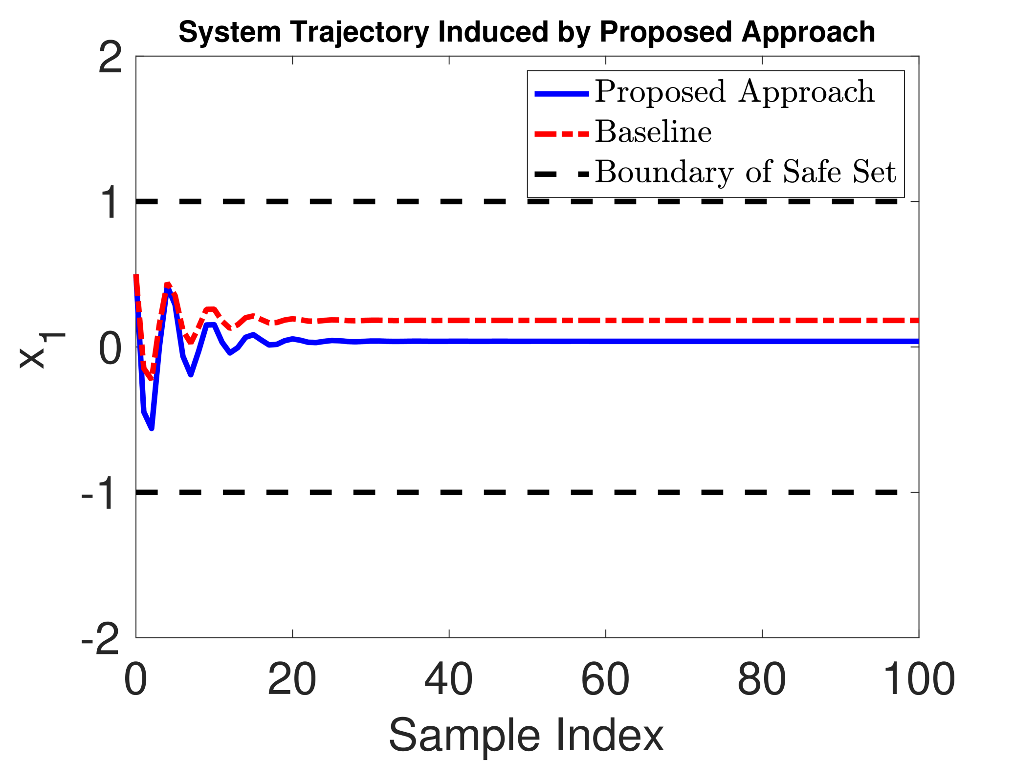
Figure 1: The trajectory induced by the proposed approach.

In this section, we present a numerical case study on the control synthesis for a DC motor. The system follows a control affine dynamics as follows [24]

$$\dot{x}=\begin{bmatrix}-39.3153x_{1}+19.1083\\ -1.6599x_{2}-3.3333\end{bmatrix}+\begin{bmatrix}-32.2293x_{2}\\ 22.9478x_{1}\end{bmatrix}u,$$

where $x_{1}$ is the rotor current, $x_{2}$ is the angular velocity, $u\in\mathcal{U}=[-4,4]$ is the stator current. The parameters in the system dynamics are unknown, and are normally obtained empirically in practice. The initial state is set as $x_{0}=[0.5,0.75]^{\top}$. The safe set of the motor is defined as $\mathcal{C}=\{x:1-x_{1}^{2}\geq 0\}$. We generate data set $R_{K}$ by randomly generating $200$ trajectories over $1000$ sampling periods, with the sampling period $\Delta t=0.01s$.

We compare our proposed approach with a baseline scenario. In the baseline scenario, the system dynamics is known. The control signal applied at each sampling time is calculated by solving the following quadratic program at each sampling time $z\Delta t$ for all $z=0,1,\ldots,$.

$$\min_{u_{z\Delta t}}~{} u_{z\Delta t}^{2}$$ (32a)

s.t. $$\frac{\partial h(x)}{\partial x}f(x)+\frac{\partial h(x)}{\partial x}g(x)u_{z\Delta t}+\alpha(h(x))\geq 0$$ (32b)

In Fig. 1, we present the trajectory generated using the proposed approach and the baseline. The trajectory generated using the proposed approach and the baseline are plotted using the blue solid line and the red dash-dotted line, respectively. We observe that both the proposed approach and the baseline guarantee safety of the system. However, the trajectories are not identical. There are two major reasons causing the trajectories to be different from each other. First, the system dynamics are not known when implementing the proposed approach, and thus the CBF constraints given in (29) are used, while the baseline implements the CBF constraint given in (32b). Second, the baseline aims at minimizing the energy used by the controller, i.e., solving quadratic program in (32) at each sampling time, while the unknown system dynamics lead to a non-convex program presented in (28), which is solved by first solving the convex program in (30) and then searching for control signal $u$ that satisfies Lemma 5. We finally observe that the proposed approach provides some robustness compared with the baseline. That is, the trajectory generated using the proposed approach tends to stay further away from both boundaries of the safe set than the baseline.

VII Conclusion

In this paper, we studied the problem of safety-critical control synthesis for sampled-data systems with unknown dynamics. We constructed a CBF constraint to guarantee the safety during each sampling period. We evaluated the CBF constraint at each sampling time by bounding the reachable state and the unknown system dynamics. We formulated a non-convex program subject to the CBF constraint to calculate the safe control input. We decomposed the non-convex program into two sub-problems with only convex programs involved. We proved the synthesized controller guarantees the safety of the unknown sampled-data system. Our proposed solution was evaluated using a numerical case study. For future work, we will incorporate a data-driven method to improve the bound of the CBF constraint by learning the nonlinear system dynamics.

Proposition 3.

Suppose Assumption 1 holds. Let $x,x^{\prime}\in\mathcal{X}$ and $u\in\mathcal{U}$. We have $\|f(x)+g(x)u-f(x^{\prime})-g(x^{\prime})u\|_{2}\leq\theta(u)\|x-x^{\prime}\|_{2}.$

Proof.

We analyze $\|f(x)+g(x)u-f(x^{\prime})-g(x^{\prime})u\|_{2}$ element-wise. Consider the $j$-th component of $f(x)+g(x)u$ and $f(x^{\prime})+g(x^{\prime})u$. We have that

$$|f_{j}(x)+(g(x)u)_{j}-f_{j}(x^{\prime})-(g(x^{\prime})u)_{j}|$$

$$\leq |f_{j}(x)-f_{j}(x^{\prime})|+|\sum_{s=1}^{m}(g_{j,s}(x)-g_{j,s}(x^{\prime}))u_{s}|$$ (33a)

$$\leq \left(L_{f_{j}}+\sum_{s=1}^{m}L_{g_{j,s}}|u_{s}|\right)\|x-x^{\prime}\|_{2},$$ (33b)

where (33a) holds by triangle inequality and matrix multiplication, and (33b) holds by Assumption 1. Given (33) holds for all $j=1,\ldots,n$, we have that the proposition holds. ∎

References

• [1] J. C. Knight, “Safety critical systems: challenges and directions,” in Proceedings of the 24th International Conference on Software Engineering, 2002, pp. 547–550.
• [2] A. D. Ames, X. Xu, J. W. Grizzle, and P. Tabuada, “Control barrier function based quadratic programs for safety critical systems,” IEEE Transactions on Automatic Control, vol. 62, no. 8, pp. 3861–3876, 2016.
• [3] L. Wang, A. D. Ames, and M. Egerstedt, “Safety barrier certificates for collisions-free multirobot systems,” IEEE Transactions on Robotics, vol. 33, no. 3, pp. 661–674, 2017.
• [4] M. H. Cohen and C. Belta, “Approximate optimal control for safety-critical systems with control barrier functions,” in IEEE Conference on Decision and Control.   IEEE, 2020, pp. 2062–2067.
• [5] A. Singletary, Y. Chen, and A. D. Ames, “Control barrier functions for sampled-data systems with input delays,” in IEEE Conference on Decision and Control.   IEEE, 2020, pp. 804–809.
• [6] W. S. Cortez, D. Oetomo, C. Manzie, and P. Choong, “Control barrier functions for mechanical systems: Theory and application to robotic grasping,” IEEE Transactions on Control Systems Technology, 2019.
• [7] J. Breeden, K. Garg, and D. Panagou, “Control barrier functions in sampled-data systems,” arXiv preprint arXiv:2103.03677, 2021.
• [8] T. Mannucci, E.-J. van Kampen, C. de Visser, and Q. Chu, “Safe exploration algorithms for reinforcement learning controllers,” IEEE Transactions on Neural Networks and Learning Systems, vol. 29, no. 4, pp. 1069–1081, 2017.
• [9] C. Folkestad, Y. Chen, A. D. Ames, and J. W. Burdick, “Data-driven safety-critical control: Synthesizing control barrier functions with Koopman operators,” IEEE Control Systems Letters, 2020.
• [10] A. Taylor, A. Singletary, Y. Yue, and A. Ames, “Learning for safety-critical control with control barrier functions,” in Learning for Dynamics and Control.   PMLR, 2020, pp. 708–717.
• [11] P. Jagtap, G. J. Pappas, and M. Zamani, “Control barrier functions for unknown nonlinear systems using Gaussian processes,” arXiv preprint arXiv:2010.05818, 2020.
• [12] L. Wang, E. A. Theodorou, and M. Egerstedt, “Safe learning of quadrotor dynamics using barrier certificates,” in 2018 IEEE International Conference on Robotics and Automation (ICRA).   IEEE, 2018, pp. 2460–2465.
• [13] F. Berkenkamp, M. Turchetta, A. Schoellig, and A. Krause, “Safe model-based reinforcement learning with stability guarantees,” in Advances in Neural Information Processing Systems, 2017, pp. 908–918.
• [14] C. Tomlin, G. J. Pappas, and S. Sastry, “Conflict resolution for air traffic management: A study in multiagent hybrid systems,” IEEE Transactions on Automatic Control, vol. 43, no. 4, pp. 509–521, 1998.
• [15] D. Mellinger, A. Kushleyev, and V. Kumar, “Mixed-integer quadratic program trajectory generation for heterogeneous quadrotor teams,” in 2012 IEEE International Conference on Robotics and Automation.   IEEE, 2012, pp. 477–483.
• [16] R. Cheng, G. Orosz, R. M. Murray, and J. W. Burdick, “End-to-end safe reinforcement learning through barrier functions for safety-critical continuous control tasks,” in Proceedings of the AAAI Conference on Artificial Intelligence, vol. 33, 2019, pp. 3387–3395.
• [17] J. Choi, F. Castañeda, C. J. Tomlin, and K. Sreenath, “Reinforcement learning for safety-critical control under model uncertainty, using control Lyapunov functions and control barrier functions,” arXiv preprint arXiv:2004.07584, 2020.
• [18] J. F. Fisac, A. K. Akametalu, M. N. Zeilinger, S. Kaynama, J. Gillula, and C. J. Tomlin, “A general safety framework for learning-based control in uncertain robotic systems,” IEEE Transactions on Automatic Control, vol. 64, no. 7, pp. 2737–2752, 2018.
• [19] J. H. Gillulay and C. J. Tomlin, “Guaranteed safe online learning of a bounded system,” in IEEE/RSJ International Conference on Intelligent Robots and Systems, 2011, pp. 2979–2984.
• [20] J. H. Gillula and C. J. Tomlin, “Guaranteed safe online learning via reachability: tracking a ground target using a quadrotor,” in IEEE International Conference on Robotics and Automation, 2012, pp. 2723–2730.
• [21] A. K. Akametalu, J. F. Fisac, J. H. Gillula, S. Kaynama, M. N. Zeilinger, and C. J. Tomlin, “Reachability-based safe learning with Gaussian processes,” in IEEE Conference on Decision and Control, 2014, pp. 1424–1431.
• [22] H. K. Khalil and J. W. Grizzle, Nonlinear Systems.   Prentice hall Upper Saddle River, NJ, 2002, vol. 3.
• [23] R. Bellman, “The stability of solutions of linear differential equations,” Duke Mathematical Journal, vol. 10, no. 4, pp. 643–647, 1943.
• [24] S. Daniel-Berhe and H. Unbehauen, “Experimental physical parameter estimation of a thyristor driven DC-motor using the HMF-method,” Control Engineering Practice, vol. 6, no. 5, pp. 615–626, 1998.