Octupolar order and Ising quantum criticality tuned by strain and dimensionality: Application to $d$-orbital Mott insulators

Abstract

Recent experiments have discovered multipolar orders in a variety of $d$-orbital Mott insulators. Motivated by uncovering the exchange interactions which underlie octupolar order proposed in the osmate double perovskites, we study a two-site model using exact diagonalization on a five-orbital Hamiltonian, incorporating spin-orbit coupling (SOC) and interactions, and including both intra-orbital and inter-orbital hopping. Using an exact Schrieffer-Wolff transformation, we then extract an effective pseudospin Hamiltonian for the non-Kramers doublets, uncovering dominant ferrooctupolar coupling driven by the interplay of two distinct intra-orbital hopping terms. Using classical Monte Carlo simulations on the face-centered cubic lattice, we obtain a ferrooctupolar transition temperature which is in good agreement with experiments on the osmate double perovskites. We also explore the impact of uniaxial strain and dimensional tuning via ultrathin films, which are shown to induce a transverse field on the Ising octupolar order. This suppresses $T_{c}$ and potentially allows one to access octupolar Ising quantum critical points. We discuss possible implications of our results for a broader class of materials which may host such non-Kramers doublet ions.

I Introduction

Multipolar orders have been extensively studied in $f$-electron compounds Santini et al. (2009); Haule and Kotliar (2009); Santini and Amoretti (2000); Paixão et al. (2002); Kiss and Fazekas (2003); Tokunaga et al. (2006); Arima (2013); Sakai and Nakatsuji (2011); Sato et al. (2012); Tsujimoto et al. (2014); Kung et al. (2015, 2016); Hattori and Tsunetsugu (2016); Freyer et al. (2018); Lee et al. (2018); Patri et al. (2019) where spin-orbit coupling and interactions dominate over weaker crystal field effects. However, there is growing evidence for such exotic “higher multipoles” in a wide range of heavy $d$-orbital metals such as LiOsO₃ and Cd₂Re₂O₇ which may exhibit odd-parity nematic orders Fu (2015); Harter et al. (2017), or quadrupolar orders as proposed in A₂OsO₄ (with A = K,Rb,Cs) Hayami et al. (2018).

Recent work from various groups have also begun to explore such orders in the Mott insulator regime, where a local picture provides a useful starting point. For $d$-orbitals in an octahedral crystal field, the $t_{2g}$ single particle levels are split by SOC, resulting in a four-fold degenerate, $j_{\rm eff}\!=\!3/2$, ground state and a doubly degenerate, $j_{\rm eff}\!=\!1/2$, excited state. These levels can realize interesting multipolar phases at different electron fillings. For instance, $d^{1}$ Mott insulators can realize the magnetism of $j_{\rm eff}=3/2$ spins. Theoretical studies of such moments on the FCC lattice have shown that they can lead to wide regimes of quadrupolar order Chen et al. (2010); Chen and Balents (2011); Svoboda et al. (2021) which may coexist with conventional dipolar magnetic order, or valence bond orders Romhányi et al. (2017). Experiments on $5d^{1}$ oxides, Ba₂NaOsO₆ with Os⁷⁺ Lu et al. (2017); Liu et al. (2018) and Ba₂MgReO₆ with Re⁶⁺ Hirai and Hiroi (2019), have found evidence for two phase transitions, with a higher temperature quadrupolar ordering transition followed by dipolar ordering at a lower temperature.

In this paper, we focus on $d^{2}$ Mott insulators, where Chen et al. (2010); Chen and Balents (2011); Svoboda et al. (2017); Lovesey et al. (2021) have argued for a local $J\!=\!2$ spin moment, which can lead to various exotic orders including quadrupolar phases. We have recently reexamined this issue Paramekanti et al. (2020); Voleti et al. (2020) and shown that virtual excitations into the high energy $e_{g}$ orbitals split the five-fold degeneracy of the $J\!=\!2$ moment as $2(E_{g})\oplus 3(T_{2g})$, resulting in a ground state non-Kramers $E_{g}$ doublet carrying quadrupolar and octupolar moments. We had proposed, on phenomenological grounds, that ferro-octupolar (FO) order of these local moments provides a comprehensive understanding Paramekanti et al. (2020); Voleti et al. (2020) of the time-reversal breaking phase transition observed in the cubic ordered double perovskite (DP) Mott insulators, Ba₂ZnOsO₆, Ba₂CaOsO₆, and Ba₂MgOsO₆, which host a $5d^{2}$ configuration on Os Thompson et al. (2014); Kermarrec et al. (2015); Thompson et al. (2016); Marjerrison et al. (2016); Maharaj et al. (2020). It is tempting to speculate that this Ising ferro-octupolar order might provide a template for storing information. Interestingly, our theory of octupolar order is reminiscent of, but distinct from, an old proposal by van den Brink and Khomskii van den Brink and Khomskii (2001) of “complex $e_{g}$ orbital” order in the colossal magnetoresistive manganites, which explored time-reversal breaking in the single-particle $e_{g}$ orbitals.

Despite the seeming success of our proposal, our previous work did not fully identify the microscopic origin of the octupolar exchange, although it did correctly identify the mechanism by which quadrupolar exchange can get suppressed. In particular, there was no theoretical basis starting from a model of interacting spin-orbit coupled electrons. This gap has been partially filled by a very recent study which combines density functional theory (DFT) and dynamical mean field theory (DMFT) calculations Pourovskii et al. (2021), and finds unequivocal evidence of FO exchange - however, it is still desirable to clarify the origin of FO order using a model tight-binding Hamiltonian. Meanwhile, several competing theories have emerged for the phase transition observed in these osmates. One proposal argues for antiferro-octupolar ordering of the $E_{g}$ doublets Lovesey and Khalyavin (2020). Other studies have argued for antiferro-quadrupolar orders based on a second-order perturbation theory calculation of the exchange interactions between non-Kramers doublets, while also including coupling to Jahn-Teller active phonons Khaliullin et al. (2021); Churchill and Kee (2021). However, the latter results do not naturally explain the time-reversal symmetry breaking observed in experiments. Motivated by these developments, we consider here a five-orbital model for two neighboring sites, which we solve using numerical exact diagonalization (ED) to extract the exchange interactions. We find dominant FO exchange, in qualitative agreement with the DFT and DMFT study Pourovskii et al. (2021), and identify a combination of two distinct intra-orbital hoppings as the driving force for FO exchange. Our results for the weaker quadrupolar terms do not precisely match the DFT and DMFT study Pourovskii et al. (2021); we attribute these differences to differences in methodology. However, our ED results are strikingly different from the simple second-order perturbation projected to the $E_{g}$ doublets which finds dominant quadrupolar exchange Khaliullin et al. (2021); Churchill and Kee (2021). We show that this discrepancy arises from the strong influence of the energetically close $T_{2g}$ triplets, which necessitates including higher order terms. Armed with our ED results, we use Monte Carlo (MC) simulations to explore the phase diagram as we vary the inter-orbital and intra-orbital hoppings. Over a wide regime of parameters, we find robust ferro-octupolar order with high $T_{c}$, thus providing an explanation for experimental observations on the double perovskite osmates. We also investigate the impact of uniaxial strain and dimensionality, showing that this leads to a transverse field on the Ising octupolar order, allowing one to tune $T_{c}$ and potentially access octupolar Ising quantum critical points. Our study extends previous work showing strain-tuning of nematic (quadrupolar) order and its transverse field quantum criticality Maharaj et al. (2017).

This paper is organized as follows. In Section II we discuss the single-site and two-site exact diagonalization results for the full five-orbital model, and show how we extract the pseudospin exchange model using an exact Schrieffer-Wolff transformation. Our results yield large swaths of parameter space with dominant FO exchange interactions on the face-centered cubic (FCC) lattice. In Section III, we discuss MC simulations of this pseudospin model, and show that it leads to a phase transition into the FO ordered state with $T_{c}$ in reasonable agreement with experiments on Ba₂ZnOsO₆, Ba₂CaOsO₆, and Ba₂MgOsO₆. Section IV studies the impact of uniaxial strain and dimensional tuning via thin films, showing that it leads to an effective transverse field on the Ising FO order, suppressing $T_{c}$ and driving the system towards an Ising quantum critical point. Section V presents the summary and outlook.

II Pseudospin Hamiltonian

II.1 Single-site exact diagonalization study

The single-site model for the $d^{2}$ configuration incorporating both crystal-field effects, electron-electron interactions, and spin-orbit coupling, has been carefully explored in our previous work. To keep our discussion self-contained, we sketch the main results. We employ a single-site (local) Hamiltonian:

$$H_{\rm loc}=H_{\rm CEF}+H_{\rm SOC}+H_{\rm int}$$ (1)

which includes $t_{2g}-e_{g}$ crystal field splitting, SOC, and electronic interactions, written in the orbital basis ($\{yz,xz,xy\},\{x^{2}\!-\!y^{2},3z^{2}\!-\!r^{2}\})\leftrightarrow(\{1,2,3\},\{4,5\}$) where $\alpha\equiv\{1,2,3\}$ label $t_{2g}$ orbitals and $\alpha\equiv\{4,5\}$ label $e_{g}$ orbitals. The CEF term is given by:

$$H_{\rm CEF}=V_{C}\sum_{\alpha=4,5}\sum_{s}n_{\alpha,s}$$ (2)

where $s$ is the spin. The SOC term is

$$\begin{split}H_{\rm SOC}&={\frac{\lambda}{2}}\sum_{\alpha,\beta}\sum_{s,s^{\prime}}\bra{\alpha}\mathbf{L}\ket{\beta}\cdot\bra{s}\boldsymbol{\sigma}\ket{s^{\prime}}c^{\dagger}_{\alpha s}c_{\beta s^{\prime}}\ ,\end{split}$$ (3)

where $\boldsymbol{\sigma}$ refers to the vector of Pauli matrices, and $\mathbf{L}$ are orbital angular momentum matrices. The operators $c_{\alpha s}$, $c^{\dagger}_{\alpha s}$ and $n_{\alpha s}$ destroy, create, and count the electrons with spin $s$ in orbital $\alpha$. The Kanamori interaction is given by

$$H_{\rm int} = U\sum_{\alpha}n_{\alpha\uparrow}n_{\alpha\downarrow}\!+\!\left(U^{\prime}-{J_{H}\over 2}\right)\sum_{\alpha>\beta}n_{\alpha}n_{\beta}$$

$$- \!J_{H}\sum_{\alpha\neq\beta}\mathbf{S}_{\alpha}\cdot\mathbf{S}_{\beta}+J_{H}\sum_{\alpha\neq\beta}c^{\dagger}_{\alpha\uparrow}c^{\dagger}_{\alpha\downarrow}c^{\phantom{\dagger}}_{\beta\downarrow}c^{\phantom{\dagger}}_{\beta\uparrow}$$

where $U$ and $U^{\prime}$ are the intra- and inter-orbital Hubbard interactions, $J_{H}$ is the Hund’s coupling, and $\mathbf{S}_{\alpha}=(1/2)c^{\dagger}_{\alpha s}\boldsymbol{\sigma}_{s,s^{\prime}}c^{\phantom{\dagger}}_{\alpha s^{\prime}}$. The operator $n_{\alpha}\equiv n_{\alpha\uparrow}+n_{\alpha\downarrow}$ counts the total number of electrons in orbital $\alpha$. Assuming spherical symmetry of the Coulomb interaction, we set $U^{\prime}=U-2J_{H}$ Georges et al. (2013). In this calculation, we use $V_{C}=2.2$ eV, $\lambda=0.4$ eV, $U=2.5$ eV, and $J_{H}=0.3$ eV in order to obtain a spin gap (described below) which matches values obtained by neutron studies Maharaj et al. (2020).

When the crystal field splitting $V_{C}\to\infty$, it leads to a five-fold degenerate ground state corresponding to a spin-orbit coupled $J=2$ quantum spin. For realistic finite $V_{C}$, this $J=2$ manifold is split, leading to a non-Kramers pseudospin doublet, with wavefunctions given in terms of $J_{z}$ eigenstates as:

$$|\psi_{g,\uparrow}\rangle=|0\rangle;~{}~{}~{}|\psi_{g,\downarrow}\rangle=\frac{1}{\sqrt{2}}(|2\rangle+|-2\rangle)$$ (5)

and an excited state triplet separated from the doublet by a gap $\sim 20$ meV. The states $|\psi_{g,\uparrow}\rangle,|\psi_{g,\downarrow}\rangle$ are individually time-reversal invariant. The angular momentum operators $(J_{x}^{2}-J_{y}^{2})/2\sqrt{3}$ and $-(3J_{z}^{2}-J^{2})/6$, restricted to this basis, act as Pauli matrices $(\tau_{x},\tau_{z})$, forming the two components of an XY-like quadrupolar order parameter, while $-\overline{J_{x}J_{y}J_{z}}/3$ (with overline denoting symmetrization) behaves as $\tau_{y}$, and serves as the Ising-like octupolar order parameter. We will define the corresponding pseudospin-$1/2$ operators as $\tilde{S}_{\alpha}=\tau_{\alpha}/2$. The ferro-octupolar order discussed later corresponds to all pseudospins being in the state $|\psi^{\rm oct}_{\pm}\rangle=|\psi_{g,\uparrow}\rangle\pm i|\psi_{g,\downarrow}\rangle$, with the signs reflecting the $\mathbb{Z}_{2}$ Ising character of octupolar order, and the factor of ‘$i$’ reflecting time-reversal symmetry breaking.

Our next goal is to uncover the interaction between these pseudospins on neighboring sites.

II.2 Two-site exact diagonalization calculation

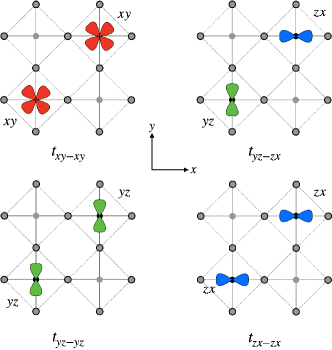
Figure 1: Schematic top-view of orbitals in the $xy$ plane showing different nearest-neighbor hoppings in the $xy$ plane. The corresponding hoppings in the $xz,yz$ planes are determined by the cubic point group symmetry.

We consider a two-site model, with each site housing a non-Kramers doublet as described above. Two sites lying in the $\gamma$ plane (where $\gamma\in\{xy,yz,zx\}$) are coupled via a hopping Hamiltonian of the form

$$H_{T}^{\gamma}=\sum_{\alpha\beta s}(T^{\gamma}_{\alpha\beta}c^{\dagger}_{2\beta s}c^{\phantom{\dagger}}_{1\alpha s}+T^{\gamma\dagger}_{\beta\alpha}c^{\dagger}_{1\alpha s}c^{\phantom{\dagger}}_{2\beta s})$$ (6)

where $T^{\gamma}$ is the hopping matrix in the $\gamma$ plane. In the $xy$ plane the sites are coupled via four hopping channels, as described in Fig. 1. The matrix in this plane takes the form

$$T^{xy}=\left(\begin{array}[]{ccc|cc}t_{yz\mbox{-}yz}&t_{yz\mbox{-}zx}&0&0&0\\ t_{zx\mbox{-}yz}&t_{zx\mbox{-}zx}&0&0&0\\ 0&0&t_{xy\mbox{-}xy}&0&0\\ \hline\cr 0&0&0&0&0\\ 0&0&0&0&0\end{array}\right)\ .$$ (12)

With cubic symmetry, the corresponding matrices in the other planes can be obtained via $C_{3}$ transformations about the [111] direction. The dominant hopping in the $xy$ plane is $t_{xy\mbox{-}xy}$, which is larger than $t_{yz\mbox{-}zx}=t_{zx\mbox{-}yz}$, which in turn is larger than $t_{yz\mbox{-}yz}=t_{zx\mbox{-}zx}$. The two-site model can be studied in the Fock space sector with four $d$ electrons having access to 20 distinct states (10 on each site). The dimension of the resulting Hilbert space is thus ${20\choose 4}=4845$. The two-site Hamiltonian

$$H^{\gamma}=H_{\rm loc}\otimes\mathcal{I}+\mathcal{I}\otimes H_{\rm loc}+H_{T}^{\gamma}$$ (13)

consists of two copies of the single-site Hamiltonian presented in Eq. 1, in addition to $H_{T}^{\gamma}$. The symbol $\mathcal{I}$ denotes the identity operator for the Hilbert space in the single-site problem.

II.3 Exact Schrieffer-Wolff transformation to obtain the pseudospin Hamiltonian

We compute the effective pseudospin Hamiltonian in the presence of intersite couplings using an exact Schrieffer-Wolff (SW) transformation Schrieffer and Wolff (1966); Bravyi et al. (2011). SW transformations in general are used to obtain effective low-energy description of a “perturbed” Hamiltonian in terms of the low-energy eigenstates of the original “unperturbed” Hamiltonian. This is accomplished by defining a so called direct rotation Bravyi et al. (2011) that connects the low-energy subspaces of the “unperturbed” and “perturbed” Hamiltonians.

For our two-site model, the intersite hoppings in Eq. 6 will serve as the source of the perturbation. Therefore, we consider the two-site decoupled Hamiltonian (Eq. 13 without $H_{T}^{\gamma}$ ) as the unperturbed Hamiltonian $H_{0}$ and the coupled model $H^{\gamma}$ (Eq. 13) as the perturbed Hamiltonian. As already discussed (Sec. II.1), the low-energy subspace of the single-site Hamiltonian has a two-fold degeneracy, which translates to a four-dimensional degenerate subspace for the decoupled two-site Hamiltonian $H_{0}$. We refer to this subspace for the decoupled (unperturbed) Hamiltonian as $\mathcal{P}_{0}$. Upon introducing intersite couplings, the subspace $\mathcal{P}_{0}$ gets modified perturbatively to a different four-dimensional subspace $\mathcal{P}$. This new subspace $\mathcal{P}$ is by definition the low-energy eigenspace for the coupled two-site Hamiltonian $H^{\gamma}$.

The SW transformation that rotates the subspace $\mathcal{P}$ to $\mathcal{P}_{0}$ is defined as the unitary transformation

$$U_{\mathcal{P}\to\mathcal{P}_{0}}=\sqrt{(2P_{0}-\mathbf{1})(2P-\mathbf{1})},$$ (14)

where $P=\sum_{\phi\in\mathcal{P}}\ket{\phi}\bra{\phi}$, $P_{0}=\sum_{\psi_{0}\in\mathcal{P}_{0}}|\psi\rangle\langle\psi|$ are the projection operators onto the subspace $\mathcal{P}$ and $\mathcal{P}_{0}$ respectively, and $\mathbf{1}$ is the identity operator. The square root in Eq. 14 is defined using a branch cut on the complex plane such that $\sqrt{1}=1$. The states $\{\ket{\phi}\}$ denote a choice of basis spanning $\mathcal{P}$ and $\{\ket{\psi}\}$ is a basis for $\mathcal{P}_{0}$. The operator $U_{\mathcal{P}\to\mathcal{P}_{0}}$ by construction maps a state $\ket{\phi}\in\mathcal{P}$ to a unique state $\ket{\psi}\in\mathcal{P}_{0}$, such that $U_{\mathcal{P}\to\mathcal{P}_{0}}\ket{\phi}=\ket{\psi}$. Consequently, $U_{\mathcal{P}\to\mathcal{P}_{0}}^{\dagger}$ does the opposite, i.e., $U_{\mathcal{P}\to\mathcal{P}_{0}}^{\dagger}\ket{\psi}=\ket{\phi}$. Furthermore, $U_{\mathcal{P}\to\mathcal{P}_{0}}$ is guaranteed to be unique iff $U_{\mathcal{P}\to\mathcal{P}_{0}}^{2}$, i.e. $(2P_{0}-\mathbf{1})(2P-\mathbf{1})$, does not have any eigenvalues that reside on the negative real axis of the complex plane. It has been shown Bravyi et al. (2011) that this is indeed the case when the corrections arising from the perturbation are sufficiently small compared with the spectral-gap $\Delta$ separating the low-energy subspace $\mathcal{P}_{0}$ from the excited states of the unperturbed Hamiltonian $H_{0}$. For our two-site model, as discussed below, we have checked that the perturbative level-shifts are weak compared with the spectral-gap $\Delta$ separating the non-Kramer’s doublet (Eq. 5) from rest of the spectrum, justifying a pseudospin-$1/2$ model of the low energy two-site spectrum.

Usually a direct computation of $U_{\mathcal{P}\to\mathcal{P}_{0}}$ (see Eq. 14) is extremely difficult in a many-body setting, since a full computation of the perturbed subspace $\mathcal{P}$, spanning all orders of perturbation, is hard due to the exponential complexity of the many-body problem. Therefore, a series expansion for $U_{\mathcal{P}\to\mathcal{P}_{0}}$ in powers of perturbation strength is often used as an approximation. However, for our two-site problem the dimension of the many-body Fock space is 4845 (see discussion above Eq. 13), and well within reach of exact diagonalization (ED) techniques. This allows us to solve for the low energy subspace $\mathcal{P}$ ($\mathcal{P}_{0}$) for the perturbed (unperturbed) Hamiltonian exactly, and obtain $U_{\mathcal{P}\to\mathcal{P}_{0}}$ using Eq. 14 to all orders of perturbation in intersite couplings.

We then use the computed SW transformation $U_{\mathcal{P}\to\mathcal{P}_{0}}$ to obtain the effective low energy form of the perturbed Hamiltonian $H^{\gamma}$ in the original subspace $\mathcal{P}_{0}$ of the unperturbed problem, as follows

$$H_{\text{eff}}^{\gamma}=\left(P_{0}U_{\mathcal{P}\to\mathcal{P}_{0}}\right)H^{\gamma}\left(U_{\mathcal{P}\to\mathcal{P}_{0}}^{\dagger}P_{0}\right).$$ (15)

Since we use the exact SW transformation $U_{\mathcal{P}\to\mathcal{P}_{0}}$ to compute $H_{\text{eff}}^{\gamma}$, the resulting $4\times 4$ Hamiltonian is also exact in the sense that it has contributions from all orders of perturbation. By construction, the eigenvalues of $H_{\text{eff}}^{\gamma}$ are precisely equal to the lowest four eigenvalues of $H^{\gamma}$.

Having proposed the strategy to extract $H_{\text{eff}}^{\gamma}$, we need to compute the effective $4\times 4$ Hamiltonian in a basis that will naturally allow us to interpret $H_{\text{eff}}^{\gamma}$ in the form of a valid pseudospin Hamiltonian. Therefore, we carry out the entire computation discussed above, using a basis spanning $\mathcal{P}_{0}$ in which the operators $(J_{x}^{2}-J_{y}^{2})$, $-\overline{J_{x}J_{y}J_{z}}$, $(3J_{z}^{2}-J^{2})$ on sites $i=1,2$, admit the Pauli matrix representations $\tau_{x}\otimes\tau_{0}$, $\tau_{y}\otimes\tau_{0}$, $\tau_{z}\otimes\tau_{0}$ and $\tau_{0}\otimes\tau_{x}$, $\tau_{0}\otimes\tau_{y}$, $\tau_{0}\otimes\tau_{z}$, respectively, where $\tau_{0}$ is the $2\times 2$ identity matrix. The steps that go into selecting such a basis for $\mathcal{P}_{0}$ are discussed in App. A. The resulting pseudospin Hamiltonian of the $\gamma$ plane in this basis takes the general form:

$$H_{\text{spin}}^{\gamma}=\tilde{\mathbf{S}}^{\top}_{1}\mathcal{K}^{\gamma}\tilde{\mathbf{S}}_{2}+\mathbf{h}_{1}^{\gamma}\cdot\tilde{\mathbf{S}}_{1}+\mathbf{h}_{2}^{\gamma}\cdot\tilde{\mathbf{S}}_{2},$$ (16)

where the symbols $\tilde{\mathbf{S}}_{i=1,2}\equiv[\tilde{S}_{ix},\tilde{S}_{iy},\tilde{S}_{iz}]$ represent the pseudospin operators for the two sites $i=1,2$. The effective “spin-spin” interactions are encoded in the $3\times 3$ $\mathcal{K}^{\gamma}$ tensor and $\mathbf{h}_{i}^{\gamma}$ are effective time-reversal even “Zeeman” fields acting on the pseudospins. Both, the $\mathcal{K}^{\gamma}$ tensor and the components of the fields $\mathbf{h}_{i}^{\gamma}$, can be obtained from the exactly computed $H_{\text{eff}}^{\gamma}$ as follows

$$\begin{split}\mathcal{K}^{\gamma}_{\alpha\beta}&=\mathrm{Tr}~{}[H_{\text{eff}}^{\gamma}\left(\tau_{\alpha}\otimes\tau_{\beta}\right)]\\ (\mathbf{h}^{\gamma}_{1})_{\alpha}&=\mathrm{Tr}~{}[H_{\text{eff}}^{\gamma}\left(\tau_{\alpha}\otimes\tau_{0}\right)]/2\\ (\mathbf{h}^{\gamma}_{2})_{\alpha}&=\mathrm{Tr}~{}[H_{\text{eff}}^{\gamma}\left(\tau_{0}\otimes\tau_{\alpha}\right)]/2\end{split}\ .$$

While the “Zeeman” fields appear to break the cubic symmetry of the lattice, they appear precisely because we consider one bond at a time (Fig. 1, for example, shows only the bond in the $xy$ plane), a process which does not respect cubic symmetry. When summed over all the neighbours of the FCC lattice, the net field vanishes exactly, i.e.

$$\sum_{\gamma\in\{xy,yz,zx\}}\mathbf{h}_{i}^{\gamma}=0\ ,$$

thus restoring the full symmetry. In Sec. IV, we will consider the impact of uniaxial strain or crystal surfaces, which will give rise to situations where the net “Zeeman” field on the pseudospin does not vanish (which is to be expected, since the strain explicitly breaks cubic symmetry and intersite couplings can then lift the pseudospin degeneracy).

II.4 Exchange couplings

Figure 2: Evolution of couplings in $xy$ plane as a function of the intra-orbital $yz$-$yz$ and $zx$-$zx$ hopping. The dashed lines show the phases based on the most dominant couplings. This cut was made for $t_{xy\mbox{-}xy}\!=\!-150$ meV and $t_{yz\mbox{-}zx}\!=\!30$ meV.

The symmetry considerations outlined in App. B dictate that the pseudospin Hamiltonian in the $xy$ plane is an $XYZ$ model:

$$H_{\rm spin}^{xy}=\mathcal{K}_{Qx}\tilde{S}_{1x}\tilde{S}_{2x}+\mathcal{K}_{Qz}\tilde{S}_{1z}\tilde{S}_{2z}+\mathcal{K}_{O}\tilde{S}_{1y}\tilde{S}_{2y}\ ,$$ (17)

where $\mathcal{K}_{Qx}$ and $\mathcal{K}_{Qz}$ are the quadrupole-quadrupole couplings, and $\mathcal{K}_{O}$ is the octupole-octupole coupling. For bonds in other planes, the exchange couplings may be obtained using $C_{3}$ rotations about the (111) axis, and they involve off-diagonal symmetric couplings of the form $(\tilde{S}_{1x}\tilde{S}_{2z}+\tilde{S}_{1z}\tilde{S}_{2x})$. In this section, we will drop the Zeeman field terms from Eq. 16, since they cancel out upon summing over all neighbors as outlined at the end of Sec. II.3. Keeping the dominant $t_{xy\mbox{-}xy}$ hopping fixed at $-150$ meV, we vary $t_{yz\mbox{-}zx}$ and $t_{yz\mbox{-}yz}=t_{zx\mbox{-}zx}$ in the ranges $0\!-\!30$ meV and $0\!-\!10$ meV, respectively, to study the dominant order hosted by the pseudospin models. We do so by analyzing the dependence of the couplings, $\mathcal{K}_{Qx}$, $\mathcal{K}_{Qz}$ and $\mathcal{K}_{O}$ on the hopping terms $t_{yz\mbox{-}yz}$ and $t_{yz\mbox{-}zx}$. Fig. 2 shows a representative example of this analysis when $t_{yz\mbox{-}zx}=\ 30$ meV. As a first pass at identifying the phases in the model, we simply assign phases based on the dominant coupling in the $XYZ$ model - an approach that will be corroborated below by classical MC simulations in Sec. III. The three phases that appear in this phase diagram spanned by the subdominant hoppings are:

1. ​​ Ferro-Octupolar (FO): $\mathcal{K}_{O}\!<\!0$

2. ​​ Antiferro-Octupolar (AFO): $\mathcal{K}_{O}\!>\!0$

3. ​​ Antiferro-Quadrupolar (AFQ): $\!\mathcal{K}_{Q\alpha}\!\!>\!\!0$ ($\alpha\!\in\!\{x,z\}$).

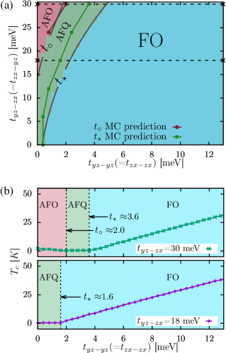
Figure 3: (a) Phase diagram in subdominant hopping parameter space, using a fixed $t_{xy-xy}=-150$ meV. The solid black phase boundaries $t_{\circ}$ and $t_{\star}$ denote the AFO-AFQ and AFQ-FO phase transition boundaries calculated simply by considering the dominant coupling (as outlined in Sec. II.4). The colored lines (represented with symbols – $\bullet$, $\blacksquare$) denote the phase boundaries obtained from MC simulations (as outlined in Sec. III). The MC predictions of the $t_{\star}$ boundary occur at smaller values of $t_{yz-zx}$, likely because the frustration of the quadrupoles on the FCC lattice causes the unfrustrated ferro-octupolar (FO) order to be preferentially stabilized despite the coupling having a smaller magnitude. (b) Representative cuts along the $y$-axis of the phase diagram (denoted as dashed-horizontal lines in (a)), showing the evolution of the critical temperature $T_{c}$ with $t_{yz-yz}$. Three piecewise regions, representing the indicated phases, can be observed. It can be seen that the values of $T_{c}$ for the AFO ($0<T_{c}<3K$) and AFQ ($0<T_{c}<1K$) phases are far lower than the $T_{c}$ values of 30-50$K$ reported in experiments, while the $T_{c}$ for the FO phase fits well with experiments.

In Fig. 3(a), we lay out the full phase diagram in the $t_{yz\mbox{-}yz}-t_{yz\mbox{-}zx}$ plane and label the phases appropriately by identifying the dominant coupling. Interestingly, we see that the FO phase forms the largest and most robust swath of the phase diagram centered around Fig. 3(a). Previous proposals have argued for the stabilization of both AFO and AFQ phases, and while these phase do exist in our model, we will show in Sec. III that for the reasonable choice of hopping parameters used, they have critical temperatures that are incompatible with experimental evidence. The specific quadrupolar ordering patterns coming from these frustrated interactions have been explored in previous works Lovesey and Khalyavin (2020); Khaliullin et al. (2021).

II.5 Comparison of exact and second-order perturbation theory results

One might reasonably wonder why it is necessary to use the ED and Schrieffer-Wolff method to extract the exchange couplings between the non-Kramers doublets, which goes beyond the standard second-order perturbation theory Khaliullin et al. (2021). In order to understand this, we note that while the charge gap is indeed much larger than the hopping energy scale, there is a small scale corresponding to the splitting between the non-Kramers ground state doublet and the excited triplet. Due to this small scale, hopping processes which involve an intermediate hopping to the triplet before returning to the doublet become significant. In perturbation theory, such processes occur at fourth order; a simple second order treatment completely misses these effects. As the energy splitting becomes smaller, it is conceivable that even higher order processes may become significant. To illustrate this point, we show in Fig. 4 the evolution of the coupling constants as a function of the dominant hopping $t_{xy-xy}$. It is clear that the second order perturbation theory agrees with the exact calculation for small $t_{xy-xy}$, but a further increase of $t_{xy-xy}$ leads to a suppression of the quadrupolar interactions which is not captured by second order perturbation theory; this suppression leads to the dominance of the ferro-octupolar exchange.

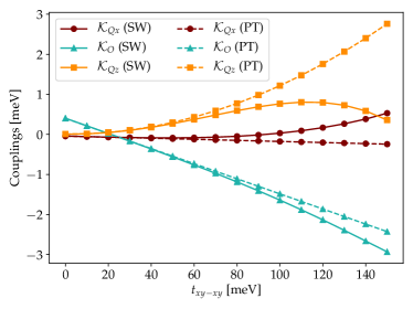
Figure 4: Comparison of the exchange couplings computed using the Schrieffer-Wolff (SW, solid lines) method and second order Perturbation Theory (PT, dashed lines). It can be seen that a second order treatment agrees with the SW results for small $t_{xy-xy}$, but would lead to the erroneous conclusion that the antiferromagnetic quadrupolar interactions would prevail, while in reality it gets suppressed and causes the ferro-octupolar interaction to dominate. We have fixed $t_{yz-zx}=18$ meV and $t_{yz-yz}=t_{zx-zx}=10$ meV.

III Monte Carlo simulations on the face-centered cubic lattice

In this section, we discuss the phase diagram of the pseudospin-$1/2$ Hamiltonian in Eq. 17, with coupling constants derived from microscopics, by treating the pseudospins as classical moments, and using MC simulations to extract their ordering and thermal phase transitions. Such an approach is expected to qualitatively capture the phase diagram on the 3D face-centered cubic lattice of the ordered double perovskites; quantum fluctuations may lead to quantitative corrections to the phase boundaries and transition temperatures.

Figure 5: Representative example of MC simulation, for the hopping parameters corresponding to the Ferro-Octupolar (FO) phase. It can be seen that there is a single phase transition, marked by a peak in the specific heat ($C_{V}$) and the emergence of a ferro-octupolar order parameter $\langle\tau_{y}\rangle$.

The simulations were conducted using the SpinMC package Buessen on a cluster of 1331 spins ($11\times 11\times 11$ primitive FCC cluster) with periodic boundary conditions, over a temperature range of $0.01$ to $10$ meV (corresponding to $0.116$ to $116$ K). To construct a phase diagram, pseudospin Hamiltonians were generated using a fixed dominant hopping $t_{xy-xy}=-150$ meV, and varying $t_{yz-zx}$ and $t_{yz-yz}$ in the ranges $0\!-\!30$ meV and $0\!-\!20$ meV, respectively (DFT studies on these and other $5d$ double perovskites have shown that these are reasonable choices Revelli et al. (2019); Churchill and Kee (2021)). We observe, in each case, a single thermal phase transition marked by a sharp peak in the specific heat $C_{V}$, and accompanied by the development of a nonzero order parameter as illustrated for a ferro-octupolar transition in Fig. 5. This representative plot was generated using hopping parameters close to those recently obtained using ab initio electronic structure calculations Churchill and Kee (2021) on the osmate double perovskites.

To identify phase boundaries shown in the full phase diagram in Fig. 3(a), we look at the development of the critical temperature $T_{c}$ as a function of the hoppings $t_{yz-zx}$ and $t_{yz-yz}$ (see Fig. 3(b)), and identify kinks, suggesting a change in the underlying analytic form of the dependence. The phase boundaries (shown with solid-lines and symbols in Fig. 3(a)) obtained using this method match well with the “naïve” method of computing the phase boundaries ($t_{\circ}$, $t_{\star}$ in Fig. 3(a)) described in Sec. II.4, where we simply looked at the dominant term in the pseudospin Hamiltonian.

IV Tuning octupolar order via uniaxial strain or dimensionality

The multipolar orders we have obtained above are highly sensitive to the nature of the inter-orbital and intra-orbital hoppings as discussed above. In addition, we have seen that the full cubic point group symmetry leads to a cancellation of the time-reversal even “field” terms acting on the $(\tau_{x},\tau_{z})$ pseudospin components, leaving us with only two-spin exchange terms. Motivated by tuning the multipolar orders, we next consider the impact of breaking cubic symmetry via strain or interfaces on the pseudospin Hamiltonian.

IV.1 Uniaxial strain

Let us consider uniaxial strain along the (001) axis ($z$-axis), which we take into account by rescaling all the inter-site hoppings for neighbors in the $xz$ and $yz$ planes by a factor $(1-\delta)$, with $\delta>0$ corresponding to tensile strain and $\delta<0$ corresponding to compressive strain. Given the typical strong dependence of the hopping amplitudes on the lattice constants Grosso and Piermarocchi (1995); Liu et al. (2017), we expect the lattice strain $\varepsilon_{zz}\ll\delta$. A careful account of strain effects must rely on experiments and ab initio electronic structure calculations, in order to relate $\delta$ to changes in lattice constants, and to examine changes in the relative strengths of the inter-orbital and intra-orbital terms; we defer this to a future study. We repeat the two-site exact diagonalization and Schrieffer-Wolff procedure as a function of $\delta$, and find that $\delta\neq 0$ leads to a non-cancelling “field” acting on the $(\tau_{x},\tau_{z})$ pseudospin components due to loss of cubic symmetry. This “field” is transverse to the octupolar ordering direction $\tau_{y}$, and can thus induce quantum fluctuations which can suppress $\langle\tau_{y}\rangle$, and potentially reveal a three-dimensional (3D) octupolar Ising quantum critical point.

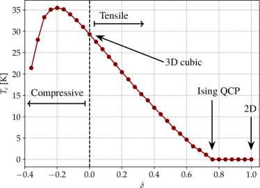
Figure 6: Evolution of the ferro-octupolar transition temperature, $T_{c}$, as a function of the hopping distortion $\delta$ induced by uniaxial strain. The cubic hopping parameters used here are $t_{xy-xy}=-150$ meV, $t_{yz-zx}=18$ meV, and $t_{yz-yz}=10$ meV.

Fig. 6 shows the $T_{c}$ computed using MC simulations with the modified exchange couplings and induced “Zeeman field” in the presence of strain. We find that tensile strain ($\delta>0$) leads to a strong suppression of $T_{c}$, due to combined effect of the weakening of octupolar exchange interactions in the $yz,zx$ planes and the generated transverse field. On the other hand, for compressive strain ($\delta<0$), $T_{c}$ first increases, since the enhancement of the octupolar exchange coupling is initially more significant than the generated transverse field, before it begins to drop. For tensile strain, we find that the (mean-field) 3D Ising quantum critical point is at $\delta_{c}\approx 0.8$, beyond which the octupolar ordering is suppressed. While this critical point $\delta_{c}$ may not be accessible in experiments, the $\delta$-dependence of $T_{c}$ at smaller strain may be more easily tested. We note again that the strain $\varepsilon_{zz}\ll\delta$.

Previous work has shown that shear strain can act as a transverse field on Ising nematic order and drive a nematic quantum phase transition Maharaj et al. (2017). Our work generalizes this idea to the case of octupolar order. Our work also goes beyond previous studies which have explored the interplay of weak magnetic field and strain for probes of octupolar ordering or octupolar susceptibility Patri et al. (2019); Sorensen and Fisher (2021).

IV.2 Ultrathin films

The generation of “Zeeman fields” when symmetry is lowered from cubic also happens naturally at surfaces or interfaces. In particular, let us consider an ultrathin (001) epitaxial film where the top and bottom faces experience a field $\propto\tau_{z}$ due to reduced symmetry. If this surface field is sufficiently strong, and the film thickness is sufficiently small, the transverse surface field can kill the octupolar order in the entire film.

In order to properly take into account the effective fields that may appear at the surfaces, it is important to ensure that all the possible interactions which break cubic symmetry on a single bond are taken into account. In the preceding sections, we had not included intersite Coulomb interactions; as we have explicitly checked, their inclusion has a negligible impact on the exchange couplings. However, we find that these interactions have a large effect on the effective fields $\mathbf{h}^{\gamma}$ in Eq. 16; while the Coulomb-induced terms cancel in the bulk when we add up the contributions from the twelve nearest-neighbors, this cancellation does not occur at surfaces. In what follows, we incorporate these residual inter-site Coulomb interactions and extract the transverse fields at the surface; the calculation of these Coulomb matrix elements for the osmate double perovskites is described in App. C.

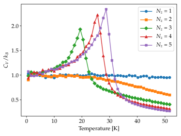
Figure 7: Evolution of the ferro-octupolar phase transition as a function of film thickness $N_{z}$. The specific heat peak marking the transition indicates that $T_{c}$ decreases with film thickness, eventually vanishing for $N_{z}\leq 2$; see text for details.

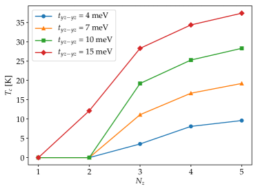
Figure 8: Evolution of the critical temperature, $T_{c}$, as a function of the film thickness, $N_{z}$, for various values of $t_{yz\mbox{-}yz}$.

With the above consideration in place, we consider a $12\times 12\times N_{z}$ lattice, with periodic boundary conditions along the $x$ and $y$ directions, and open boundary conditions along the $z$ direction. Here $N_{z}$ represents the film thickness. We incorporate the microscopically computed effective transverse fields on the top and bottom faces of the film. For illustrative purposes, we fix two hopping parameters, $t_{xy-xy}=-150$ meV, $t_{yz-zx}=18$ meV, and vary $t_{yz-yz}$. Fig. 7 shows (for $t_{yz-yz}=10$ meV) the evolution of the specific heat, $C_{V}$, as we decrease the film thickness $N_{z}$. Fig. 8 shows how $T_{c}$, extracted from the peak in the specific heat, changes as we vary $N_{z}$ for various values of $t_{yz-yz}$. It can be seen that for a wide range of values of this hopping parameter, we are able to completely suppress $T_{c}$ for bilayer samples. We thus see that as we decrease the film thickness, we will tune the system through a 2D Ising quantum critical point. This provides another promising avenue to suppress $T_{c}$ and to look for signatures of octupolar quantum criticality.

V Discussion

We have discussed a simple tight-binding model with spin-orbit coupling and interactions which leads to ferro-octupolar order in the ordered double perovskite osmates Ba₂ZnOsO₆, Ba₂CaOsO₆, and Ba₂MgOsO₆. Our calculations, which use exact diagonalization and an exact Schrieffer-Wolff transformation and MC simulations, show that we can capture the octupolar order and its high transition temperature as observed in experiments. In addition, we have shown how strain and thin film geometries can induce transverse fields which suppress the octupolar ordering temperature, potentially revealing an Ising quantum critical point. Our work has implications for a broad class of materials, including $d$-orbital transition metal oxides and $f$-orbital heavy fermion systems, where such multipolar orders may be accessible. For instance, NpO₂ is a well-known example of an fcc lattice material which hosts higher-rank multipolar order with time-reversal symmetry breaking Santini et al. (2009); Haule and Kotliar (2009); Santini and Amoretti (2000); Paixão et al. (2002); Kiss and Fazekas (2003); Tokunaga et al. (2006). Octupolar order of the $T_{xyz}$ type explored here has also been proposed in the Pr(Ti,V,Ir)₂(Al,Zn)₂₀ compounds where Pr moments live on the diamond lattice Lee et al. (2018); Patri et al. (2019). In future work, it would be important to extend our work to understand the origins of multipolar order in these materials. Indeed, there may be a large set of lattice geometries where such physics of multipolar order in $d^{2}$ transition metal compounds would be worth exploring, as highlighted by Khaliullin, et al Khaliullin et al. (2021). More broadly, our work shows that understanding the impact of thin film geometries, surfaces, and interfaces, in promoting or suppressing multipolar orders in non-Kramers doublet systems may be a fruitful research direction.

Note added: During completion of this manuscript, we became aware of the recent preprint by Churchill and Kee Churchill and Kee (2021) which has partial overlap with our work. Mainly, these authors identify the combination of two different intra-orbital hoppings as favoring octupolar order, as we also independently discovered in our work. However, in significant contrast to our work which finds wide regimes of octupolar order, they find evidence for dominant quadrupolar orders. These quadrupolar orders do not naturally account for the broken time-reversal symmetry observed in the osmate double perovskites.

VI Acknowledgments

We thank F. Lasse Buessen for help with the MC simulations. We thank Giniyat Khaliullin and Hae-Young Kee for useful discussions. This work was supported by the Natural Sciences and Engineering Research Council of Canada. Exact diagonalization computations were performed on the Niagara supercomputer at the SciNet HPC Consortium. SciNet is funded by: the Canada Foundation for Innovation; the Government of Ontario; Ontario Research Fund - Research Excellence; and the University of Toronto. MC simulations were conducted on the Cedar supercomputer, one of Compute Canada’s National systems, located in Simon Fraser University.

Appendix A Choosing $\mathcal{P}_{0}$ basis states in the Schrieffer-Wolff (SW) process

An important step in the SW process is ensuring that we use basis states for $\mathcal{P}_{0}$ which can be interpreted as direct products of (pseudo)spin states on the two sites. This enables us to interpret the extracted pseudospin Hamiltonian as an direct-product type interaction between the multipole moments in the doublet manifold. While there are many ways to do this, the simplest is to leverage the fact that the $\mathcal{P}_{0}$ Hamiltonian is decoupled, meaning that the basis states can be constructed out of the single site states.

At a single site level, we can ensure that the “up” and “down” pseudospin states from Sec. II.1 correspond to eigenstates of $\tau_{z}$ ($\propto 3J_{z}^{2}-J^{2}$), by adding a term to the Hamiltonian which couples an infinitesimal magnetic field to this operator. This weakly breaks the two-fold degeneracy and the basis states of $\mathcal{P}_{0}$ can simply be built using the direct product of the aforementioned states.

Appendix B Symmetry considerations for the Pseudospin Hamiltonian

As stated in the main text, the following correspondence exists between $J=2$ angular momentum multipole moments and the Pauli matrices in the low energy non-Kramers doublet manifold:

$$\begin{split}{1\over 2\sqrt{3}}(J_{x}^{2}-J_{y}^{2})&\rightarrow\tau_{x}\\ -{1\over 3}\overline{J_{x}J_{y}J_{z}}&\rightarrow\tau_{y}\\ -{1\over 6}{(3J_{z}^{2}-J^{2})}&\rightarrow\tau_{z}\end{split}\ .$$ (18)

Therefore, the most general spin-1/2 Hamiltonian takes the form (sites are numbered 1 and 2):

$$H_{\rm spin}={1\over 4}\mathcal{K}_{ab}\left(\tau_{a}\otimes\tau_{b}\right).$$ (19)

For a bond in the $xy$ plane, the following symmetry considerations heavily constrain the form of $\mathcal{K}$:

1. Inversion symmetry about the center of the bond exchanges the site indices, implying that $\mathcal{K}$ is symmetric, i.e.

   $$\begin{split}\mathcal{K}_{xy}=\mathcal{K}_{yz}\\ \mathcal{K}_{yz}=\mathcal{K}_{zy}\\ \mathcal{K}_{zx}=\mathcal{K}_{xz}\end{split}\ .$$ (20)

2. Under the $M_{z}$ mirror transformation (the mirror plane is $z=0$), we have

   $$\begin{rcases}J_{z}\rightarrow-J_{z}\\ J_{x}\rightarrow-J_{y}\\ J_{y}\rightarrow-J_{x}\end{rcases}\implies\begin{cases}\tau_{x}\rightarrow-\tau_{x}\\ \tau_{y}\rightarrow-\tau_{y}\\ \tau_{z}\rightarrow\tau_{z}\end{cases}\ .$$ (21)

   For the above to be a symmetry of the system, we must have that $\mathcal{K}_{zx}=\mathcal{K}_{yz}=0$

3. The system is time-reversal symmetric. Under the time reversal operation we have the following transformations:

   $$\begin{split}\tau_{y}\rightarrow-\tau_{y}\\ \tau_{x},\tau_{z}\rightarrow\tau_{x},\tau_{z}\end{split}\ .$$ (22)

   This implies that $\mathcal{K}_{xy}=\mathcal{K}_{yz}=0$

The above points, when considered together, lead to the vanishing of all the off-diagonal elements in $\mathcal{K}$. This leaves us with an $XYZ$ Hamiltonian of the form

$$\mathcal{K}=\begin{pmatrix}\mathcal{K}_{xx}&0&0\\ 0&\mathcal{K}_{yy}&0\\ 0&0&\mathcal{K}_{zz}\end{pmatrix}\ .$$ (23)

In the main text, we have renamed $\mathcal{K}_{xx}\rightarrow\mathcal{K}_{Qx}$, $\mathcal{K}_{yy}\rightarrow\mathcal{K}_{O}$, and $\mathcal{K}_{zz}\rightarrow\mathcal{K}_{Qz}$. The exchange Hamiltonian in the $zx$ and $yz$ planes can be conveniently obtained using $C_{3}$ rotations about the cubic (111) direction.

Appendix C Intersite Coulomb matrix elements

To evaluate matrix elements for the intersite direct Coulomb interaction, we must compute integrals of the form

$$\mathcal{V}_{ab}={e^{2}\over 4\pi\kappa\epsilon_{0}}\int d\mathbf{r}\int d\mathbf{r^{\prime}}\text{ }{|\psi_{1}^{a}(\mathbf{r})|^{2}\text{ }|\psi_{2}^{b}(\mathbf{r^{\prime}})|^{2}\over|\mathbf{r}-\mathbf{r^{\prime}}|},$$ (24)

where $\kappa$ is the dielectric constant (we set $\kappa=10$), and $\psi_{1}^{a}$ ($\psi_{2}^{b}$) refers to the wavefunction of an electron in orbital $a$($b$) centered on site 1(2). We use Hydrogen-type $d$ orbital wavefunctions, of the form $\psi^{a}(\mathbf{r})=R(r)T^{a}(\theta,\phi)$, where $R(r)$ refers to the radial part of the wavefunction, and $T^{a}$ is the tesseral harmonic associated with the $a$ orbital. The detailed form of these functions for the osmate double perovskites are given in Appendix C of Ref. Voleti et al. (2020).

To compute ${\cal V}_{ab}$ in Eq. 24, we use a MC integration method. We interpret the integral as a random-walk in a 6-dimensional (6D) space; each point $\mathbf{x}$ in the 6D space is defined as $\mathbf{x}=(\mathbf{r}_{x},\mathbf{r}_{y},\mathbf{r}_{z},\mathbf{r}^{\prime}_{x},\mathbf{r}^{\prime}_{y},\mathbf{r}^{\prime}_{z})$ in terms of the original position vectors appearing in Eq. 24. The random-walk is performed obeying the rules of a Markov process guided by the joined probability distribution

$$p_{ab}(\mathbf{x}=(\mathbf{r},\mathbf{r^{\prime}}))=|\psi_{1}^{a}(\mathbf{r})|^{2}|\psi_{2}^{b}(\mathbf{r^{\prime}})|^{2}.$$ (25)

Starting from a randomly chosen $\mathbf{x}_{n=0}$, a sequence of points $\{\mathbf{x}_{0},\cdots,\mathbf{x}_{n}\}$ is generated by taking steps $\mathbf{dx}$ of a sufficiently small length in a randomly-chosen direction, so that upon acceptance of the step we get $\mathbf{x_{n+1}}=\mathbf{x}_{n}+\mathbf{dx}$. A proposed step $\mathbf{dx}$ is directly accepted if $p_{ab}(\mathbf{x}_{n}+\mathbf{dx})/p_{ab}(\mathbf{x}_{n})\geq 1$. If $p_{ab}(\mathbf{x}_{n}+\mathbf{dx})/p_{ab}(\mathbf{x}_{n})<1$, a random number $r$ is picked from the uniform distribution defined on the interval $[0,1]$. The step $\mathbf{dx}$ is accepted if the number $r\leq p_{ab}(\mathbf{x}_{n}+\mathbf{dx})/p_{ab}(\mathbf{x}_{n})$, otherwise the process is repeated for a new step $\mathbf{dx^{\prime}}$. We allow the random-walk to proceed for a large number ($O(10^{6})$) of MC steps. The value of the integral in Eq. 24 is then estimated using

$$\mathcal{V}_{ab}\approx{e^{2}\over 4\pi\kappa\epsilon_{0}}\frac{1}{N_{\text{steps}}-N_{\text{skip}}}\sum_{n=N_{\text{skip}}}^{N_{\text{steps}}}\frac{1}{|\mathbf{r}_{n}-\mathbf{r}^{\prime}_{n}|},$$ (26)

where $\mathbf{r}_{n}$ ($\mathbf{r}^{\prime}_{n}$) is the obtained from the first (last) three components of $\mathbf{x}_{n}$ and $N_{\text{steps}}$ is the number of MC steps. We also skip the first $N_{\text{skip}}$ steps to neglect transient contributions due to the choice of the initial point $\mathbf{x}_{0}$. We used $N_{\text{skip}}\sim O(10^{3})$ for our calculations. The total number of $N_{\text{steps}}$ were determined by monitoring when the fluctuations of $\mathcal{V}_{ab}$ in Eq. 26, resulting from the random-walk, reduced to less than $1\%$ of the average value.

For a pair of nearest-neighbor sites in the $xy$-plane, and working in the basis $\{yz,zx,xy,x^{2}\!-\!y^{2},3z^{2}\!-\!1\}$, we obtain the Coulomb interaction matrix(in eV):

$$\mathcal{V}=\begin{pmatrix}0.231&&0.237&&0.244&&0.239&&0.233\\ 0.237&&0.231&&0.244&&0.239&&0.233\\ 0.244&&0.244&&0.261&&0.260&&0.245\\ 0.239&&0.239&&0.260&&0.254&&0.239\\ 0.233&&0.233&&0.245&&0.239&&0.232\end{pmatrix}.$$ (27)

We note that this matrix has an orbital independent value $\sim 0.25$ eV, and orbital-dependent parts on the scale of $\sim 30$ meV. Adding this Coulomb term to the two-site Hamiltonian as $\sum_{\alpha\beta}{\mathcal{V}}_{\alpha\beta}n_{1,\alpha}n_{2,\beta}$, where $n_{i\alpha}$ is the total electron number in orbital $\alpha$ at site $i$, we use ED and the Schrieffer-Wolff method to recompute the exchange interactions and effective fields. We find that the two-site exchange interactions are nearly unaffected since the scale of ${\mathcal{V}}_{\alpha\beta}$ is much smaller than the on-site Hubbard interaction $U=2.5$ eV. However, the orbital-dependent part of ${\mathcal{V}}_{\alpha\beta}$ results in an extra effective field $\propto\tau_{z}$ on the non-Kramers doublet. To see this, we note that mean field theory yields an on-site term at site $i=1$ given by $\sum_{\alpha\beta}{\mathcal{V}}_{\alpha\beta}n_{1,\alpha}\langle n_{2\beta}\rangle$. Upon projection to the non-Kramers doublet, this acts as an extra effective field. Our computations show that the scale of this field is $\sim 8$ meV, which is larger than the field produced by two-site exchange interactions alone. Thus, while these fields cancel in the cubic bulk, the Coulomb-enhanced surface fields are strong enough to overcome the ferro-octupolar exchange and kill the octupolar order for sufficiently thin films as shown in the paper.

References

- Santini et al. (2009) P. Santini, S. Carretta, G. Amoretti, R. Caciuffo, N. Magnani, and G. H. Lander, Rev. Mod. Phys. 81, 807 (2009).
- Haule and Kotliar (2009) K. Haule and G. Kotliar, Nature Physics 5, 796 EP (2009).
- Santini and Amoretti (2000) P. Santini and G. Amoretti, Phys. Rev. Lett. 85, 2188 (2000).
- Paixão et al. (2002) J. A. Paixão, C. Detlefs, M. J. Longfield, R. Caciuffo, P. Santini, N. Bernhoeft, J. Rebizant, and G. H. Lander, Phys. Rev. Lett. 89, 187202 (2002).
- Kiss and Fazekas (2003) A. Kiss and P. Fazekas, Phys. Rev. B 68, 174425 (2003).
- Tokunaga et al. (2006) Y. Tokunaga, D. Aoki, Y. Homma, S. Kambe, H. Sakai, S. Ikeda, T. Fujimoto, R. E. Walstedt, H. Yasuoka, E. Yamamoto, A. Nakamura, and Y. Shiokawa, Phys. Rev. Lett. 97, 257601 (2006).
- Arima (2013) T.-h. Arima, Journal of the Physical Society of Japan 82, 013705 (2013).
- Sakai and Nakatsuji (2011) A. Sakai and S. Nakatsuji, Journal of the Physical Society of Japan 80, 063701 (2011).
- Sato et al. (2012) T. J. Sato, S. Ibuka, Y. Nambu, T. Yamazaki, T. Hong, A. Sakai, and S. Nakatsuji, Phys. Rev. B 86, 184419 (2012).
- Tsujimoto et al. (2014) M. Tsujimoto, Y. Matsumoto, T. Tomita, A. Sakai, and S. Nakatsuji, Phys. Rev. Lett. 113, 267001 (2014).
- Kung et al. (2015) H.-H. Kung, R. E. Baumbach, E. D. Bauer, V. K. Thorsmølle, W.-L. Zhang, K. Haule, J. A. Mydosh, and G. Blumberg, Science 347, 1339 (2015).
- Kung et al. (2016) H.-H. Kung, S. Ran, N. Kanchanavatee, V. Krapivin, A. Lee, J. A. Mydosh, K. Haule, M. B. Maple, and G. Blumberg, Phys. Rev. Lett. 117, 227601 (2016).
- Hattori and Tsunetsugu (2016) K. Hattori and H. Tsunetsugu, Journal of the Physical Society of Japan 85, 094001 (2016).
- Freyer et al. (2018) F. Freyer, J. Attig, S. Lee, A. Paramekanti, S. Trebst, and Y. B. Kim, Phys. Rev. B 97, 115111 (2018).
- Lee et al. (2018) S. Lee, S. Trebst, Y. B. Kim, and A. Paramekanti, Phys. Rev. B 98, 134447 (2018).
- Patri et al. (2019) A. S. Patri, A. Sakai, S. Lee, A. Paramekanti, S. Nakatsuji, and Y. B. Kim, Nature Communications 10, 4092 (2019).
- Fu (2015) L. Fu, Phys. Rev. Lett. 115, 026401 (2015).
- Harter et al. (2017) J. W. Harter, Z. Y. Zhao, J.-Q. Yan, D. G. Mandrus, and D. Hsieh, Science 356, 295 (2017), https://science.sciencemag.org/content/356/6335/295.full.pdf .
- Hayami et al. (2018) S. Hayami, H. Kusunose, and Y. Motome, Phys. Rev. B 97, 024414 (2018).
- Chen et al. (2010) G. Chen, R. Pereira, and L. Balents, Phys. Rev. B 82, 174440 (2010).
- Chen and Balents (2011) G. Chen and L. Balents, Phys. Rev. B 84, 094420 (2011).
- Svoboda et al. (2021) C. Svoboda, W. Zhang, M. Randeria, and N. Trivedi, Phys. Rev. B 104, 024437 (2021).
- Romhányi et al. (2017) J. Romhányi, L. Balents, and G. Jackeli, Phys. Rev. Lett. 118, 217202 (2017).
- Lu et al. (2017) L. Lu, M. Song, W. Liu, A. P. Reyes, P. Kuhns, H. O. Lee, I. R. Fisher, and V. F. Mitrović, Nature Communications 8, 14407 EP (2017).
- Liu et al. (2018) W. Liu, R. Cong, E. Garcia, A. Reyes, H. Lee, I. Fisher, and V. MitroviÄ, Physica B: Condensed Matter 536, 863 (2018).
- Hirai and Hiroi (2019) D. Hirai and Z. Hiroi, Journal of the Physical Society of Japan 88, 064712 (2019).
- Svoboda et al. (2017) C. Svoboda, M. Randeria, and N. Trivedi, Phys. Rev. B 95, 014409 (2017).
- Lovesey et al. (2021) S. W. Lovesey, D. D. Khalyavin, G. van der Laan, and G. J. Nilsen, Phys. Rev. B 103, 104429 (2021).
- Paramekanti et al. (2020) A. Paramekanti, D. D. Maharaj, and B. D. Gaulin, Phys. Rev. B 101, 054439 (2020).
- Voleti et al. (2020) S. Voleti, D. D. Maharaj, B. D. Gaulin, G. Luke, and A. Paramekanti, Phys. Rev. B 101, 155118 (2020).
- Thompson et al. (2014) C. M. Thompson, J. P. Carlo, R. Flacau, T. Aharen, I. A. Leahy, J. R. Pollichemi, T. J. S. Munsie, T. Medina, G. M. Luke, J. Munevar, S. Cheung, T. Goko, Y. J. Uemura, and J. E. Greedan, Journal of Physics: Condensed Matter 26, 306003 (2014).
- Kermarrec et al. (2015) E. Kermarrec, C. A. Marjerrison, C. M. Thompson, D. D. Maharaj, K. Levin, S. Kroeker, G. E. Granroth, R. Flacau, Z. Yamani, J. E. Greedan, and B. D. Gaulin, Phys. Rev. B 91, 075133 (2015).
- Thompson et al. (2016) C. M. Thompson, C. A. Marjerrison, A. Z. Sharma, C. R. Wiebe, D. D. Maharaj, G. Sala, R. Flacau, A. M. Hallas, Y. Cai, B. D. Gaulin, G. M. Luke, and J. E. Greedan, Phys. Rev. B 93, 014431 (2016).
- Marjerrison et al. (2016) C. A. Marjerrison, C. M. Thompson, A. Z. Sharma, A. M. Hallas, M. N. Wilson, T. J. S. Munsie, R. Flacau, C. R. Wiebe, B. D. Gaulin, G. M. Luke, and J. E. Greedan, Phys. Rev. B 94, 134429 (2016).
- Maharaj et al. (2020) D. D. Maharaj, G. Sala, M. B. Stone, E. Kermarrec, C. Ritter, F. Fauth, C. A. Marjerrison, J. E. Greedan, A. Paramekanti, and B. D. Gaulin, Phys. Rev. Lett. 124, 087206 (2020).
- van den Brink and Khomskii (2001) J. van den Brink and D. Khomskii, Phys. Rev. B 63, 140416 (2001).
- Pourovskii et al. (2021) L. V. Pourovskii, D. F. Mosca, and C. Franchini, “Ferro-octupolar order and low-energy excitations in d2 double perovskites of osmium,” (2021), arXiv:2107.04493 [cond-mat.str-el] .
- Lovesey and Khalyavin (2020) S. W. Lovesey and D. D. Khalyavin, Phys. Rev. B 102, 064407 (2020).
- Khaliullin et al. (2021) G. Khaliullin, D. Churchill, P. P. Stavropoulos, and H.-Y. Kee, Phys. Rev. Research 3, 033163 (2021).
- Churchill and Kee (2021) D. Churchill and H.-Y. Kee, “Two quadrupolar orders in osmium double-perovskites,” (2021), arXiv:2109.08104 [cond-mat.str-el] .
- Maharaj et al. (2017) A. V. Maharaj, E. W. Rosenberg, A. T. Hristov, E. Berg, R. M. Fernandes, I. R. Fisher, and S. A. Kivelson, Proceedings of the National Academy of Sciences 114, 13430 (2017), https://www.pnas.org/content/114/51/13430.full.pdf .
- Georges et al. (2013) A. Georges, L. d. Medici, and J. Mravlje, Annual Review of Condensed Matter Physics 4, 137 (2013).
- Schrieffer and Wolff (1966) J. R. Schrieffer and P. A. Wolff, Phys. Rev. 149, 491 (1966).
- Bravyi et al. (2011) S. Bravyi, D. P. DiVincenzo, and D. Loss, Annals of Physics 326, 2793 (2011).
- (45) F. L. Buessen, “Spinmc.jl: Classical monte carlo simulation package for julia,” .
- Revelli et al. (2019) A. Revelli, C. C. Loo, D. Kiese, P. Becker, T. Fröhlich, T. Lorenz, M. Moretti Sala, G. Monaco, F. L. Buessen, J. Attig, M. Hermanns, S. V. Streltsov, D. I. Khomskii, J. van den Brink, M. Braden, P. H. M. van Loosdrecht, S. Trebst, A. Paramekanti, and M. Grüninger, Phys. Rev. B 100, 085139 (2019).
- Grosso and Piermarocchi (1995) G. Grosso and C. Piermarocchi, Phys. Rev. B 51, 16772 (1995).
- Liu et al. (2017) Y.-C. Liu, F.-C. Zhang, T. M. Rice, and Q.-H. Wang, npj Quantum Materials 2, 12 (2017).
- Sorensen and Fisher (2021) M. E. Sorensen and I. R. Fisher, Phys. Rev. B 103, 155106 (2021).