![[Uncaptioned image]](/html/2109.13237/assets/figures/uofi.png)
University of Illinois at Urbana-Champaign
Department of Mathematics
Department of Computer Science
UNDERGRADUATE THESIS
Submitted as part of an undergraduate research program
DOODLER: Determining Out-Of-Distribution
Likelihood from Encoder Reconstructions
Acknowledgements
I would like to begin by thanking my mom and dad for their unending and essential support, and all the other obvious reasons why anyone would thank their parents. But I must also thank them, Elliot N. Kent and Marsha N. Hahn, as individuals, unique and especial, because I get to be nobody else but their son. They taught me to be me. They taught me to learn. It is from them that I inherited my appetite for knowledge, and my desire to bend that knowledge to the world as it exists. What I have written here, being both original Scientific research and working towards real-world applications, is dedicated to them.
I would also like to thank my friend, Moira E. Iten, and her family, for their ceaseless moral support and cheering-on. It would be impossible to determine the precise extent of their contributions, but that is meaningless in the face of my appreciation for them.
I will finish by thanking my colleagues: Charles C. Wamsley, Davin Flateau, and Amber Ferguson, and all the other folks at Ball Aerospace & Technologies Corp., for the excellent and interesting technical conversations, the insight into the problems faced in the real-world practice of Machine Learning, and the opportunity to develop as a Researcher and Engineer.
“A little song, a little dance, a little seltzer down your pants.” -Tim
1 Abstract
Deep Learning models possess two key traits that, in combination, make their use in the real world a risky prospect. One, they do not typically generalize well outside of the distribution for which they were trained, and two, they tend to exhibit confident behavior regardless of whether or not they are producing meaningful outputs. While Deep Learning possesses immense power to solve realistic, high-dimensional problems, these traits in concert make it difficult to have confidence in their real-world applications. To overcome this difficulty, the task of Out-Of-Distribution (OOD) Detection has been defined, to determine when a model has received an input from outside of the distribution for which it is trained to operate.
This paper introduces and examines a novel methodology, DOODLER, for OOD Detection, which directly leverages the traits which result in its necessity. By training a Variational Auto-Encoder (VAE) on the same data as another Deep Learning model, the VAE learns to accurately reconstruct In-Distribution (ID) inputs, but not to reconstruct OOD inputs, meaning that its failure state can be used to perform OOD Detection. Unlike other work in the area, DOODLER requires only very weak assumptions about the existence of an OOD dataset, allowing for more realistic application. DOODLER also enables pixel-wise segmentations of input images by OOD likelihood, and experimental results show that it matches or outperforms methodologies that operate under the same constraints.
2 Introduction
Perhaps the most fundamental of all questions in both the academic study and applied practice of Machine Learning is that of Out-Of-Distribution Generalization, or how to produce a model that is capable of operating in settings for which it has not been expressly prepared [23]. This is an extraordinarily difficult problem, and while inroads have been made in some areas like Online Learning and Meta-Learning [19, 22], it is still generally true that
-
1.
Machine Learning models are not good at generalizing outside of the domain they were trained for, and
-
2.
Machine Learning models will still express their inferences with high confidence when outside their domain [16].
The confluence of these traits means that, despite the extraordinary power of Machine and Deep Learning to crack complex, real-world, hyperdimensional problems that are intractable with any other methodology [18], actually using these models in a production environment becomes a fraught decision. This is true to an extreme degree in areas like Vehicle Autonomy, Medical Diagnostics, and Defense, where a wrong decision made confidently may result in human casualties.
Therefore, robust Out-Of-Distribution Detection, the ability to preempt the differences between laboratory and real-world conditions, to determine when a model is receiving data for which it is not prepared, is essential. By making these determinations accurately, it allows for autonomous systems to activate a backup protocol or Human-in-the-Loop system, greatly increasing their trustworthiness for applications.
3 Related Work
Much of the OOD Detection research literature available makes a number of strange assumptions; among these, the existence of a dataset consisting of Out-Of-Distribution samples to train a binary classifier [15]. To comprehensively cover what is OOD, this dataset would have to contain samples from the entirety of the space outside of the In-Distribution. If the ID contained pictures of dogs, for example, this OOD dataset would have to contain pictures of literally everything that isn’t a dog: cats, foxes, centaurs, Gaussian noise, fruit, supernovae, cartographic maps of Poland, so on and so forth. If any class of data is left out, then it is outside of the distribution for which the detector is prepared, making it necessary to perform OOD Detection in order to perform OOD Detection, leaving us back at square one. Thus, any true OOD Detector must be trained in an Unsupervised manner, without training on an OOD dataset.
Other methods, like ODIN [13], make significant progress towards achieving this. ODIN operates by comparing a classification model’s output on an input to its output when the input has a small adversarial perturbation, with the output changing less for Out-Of-Distribution inputs than In-Distribution ones. While this performs very well, it’s also much more computationally expensive, requiring two forward passes and a gradient calculation, than single-shot inference, so it’s unsuited to real-time applications. Also worth noting is that, although the model may be trained without OOD samples, the analysis of the output distributions required to differentiate between ID and OOD data requires at least a few samples. But this is a much weaker requirement than a comprehensive OOD dataset, as it’s only needed in order to determine a handful of parameters, rather than to train a model that takes them as input. As a result, ODIN can be assumed to generalize much more reasonably.
Another method, DAGMM [24], involves using a Gaussian Mixture Model on the latent space of a Variational Auto-Encoder [7]. While a classical model like a Gaussian Mixture would be unable to deal with the high dimensionality of images, the low number of dimensions of the VAE’s encodings means that it can handle much more abstract data than might otherwise be possible. This still makes a number of assumptions about the underlying distribution, including that the probability density of the latent space can be represented meaningfully by a Gaussian Mixture Model. It also imposes both a limit on the number of dimensions that can be used in the latent space, and a requirement that this number of dimensions stays constant between training, testing, and real-world inference. This is disappointing, as ordinarily fully convolutional models can be trained on smaller chips than they will be used for, making training easier. However, using VAEs for OOD Detection does get at the heart of the matter, because the underlying problem involves getting a handle on patterns in the In-Distribution, which is fundamental to how VAEs operate.
| ODIN | DAGMM | DOODLER | |
|---|---|---|---|
| Unsupervised | |||
| Chip Size Invariant | |||
| One-Shot Inference | |||
| Segmentation |
Something else worth considering is the possibility of performing segmented Out-Of-Distribution Detection on images, to help with explainability; an OOD Detector would be much more trustworthy, and provide helpful information to a Human-in-the-Loop counterpart, if it could point out exactly where in an image it was seeing something that set it off. However, the work in this area has relied extensively on the existence of OOD datasets [2, 5, 20], so it could still benefit greatly from moving to an Unsupervised setting.
But on a fundamental level, much of the available Unsupervised Out-Of-Distribution Detection research comes at it from an analytic rather than a functional perspective. Broadly, the work on the topic has thought of the defining trait of OOD data to be that they literally fall outside of the high-density region of a probabilistic In-Distribution. However, when looking at it from a functional perspective, the primary trait of OOD data is that they cause models to fail and fail confidently, this being the reason why it is valuable to detect them in the first place. By shifting over to this framework, a new methodology immediately presents itself: find some task for which a failure state can be detected without a ground truth label for comparison, and then use that failure state as a detection signal. Thus, DOODLER: Determining Out-Of-Distribution Likelihood from Encoder Reconstructions.
4 Methodology
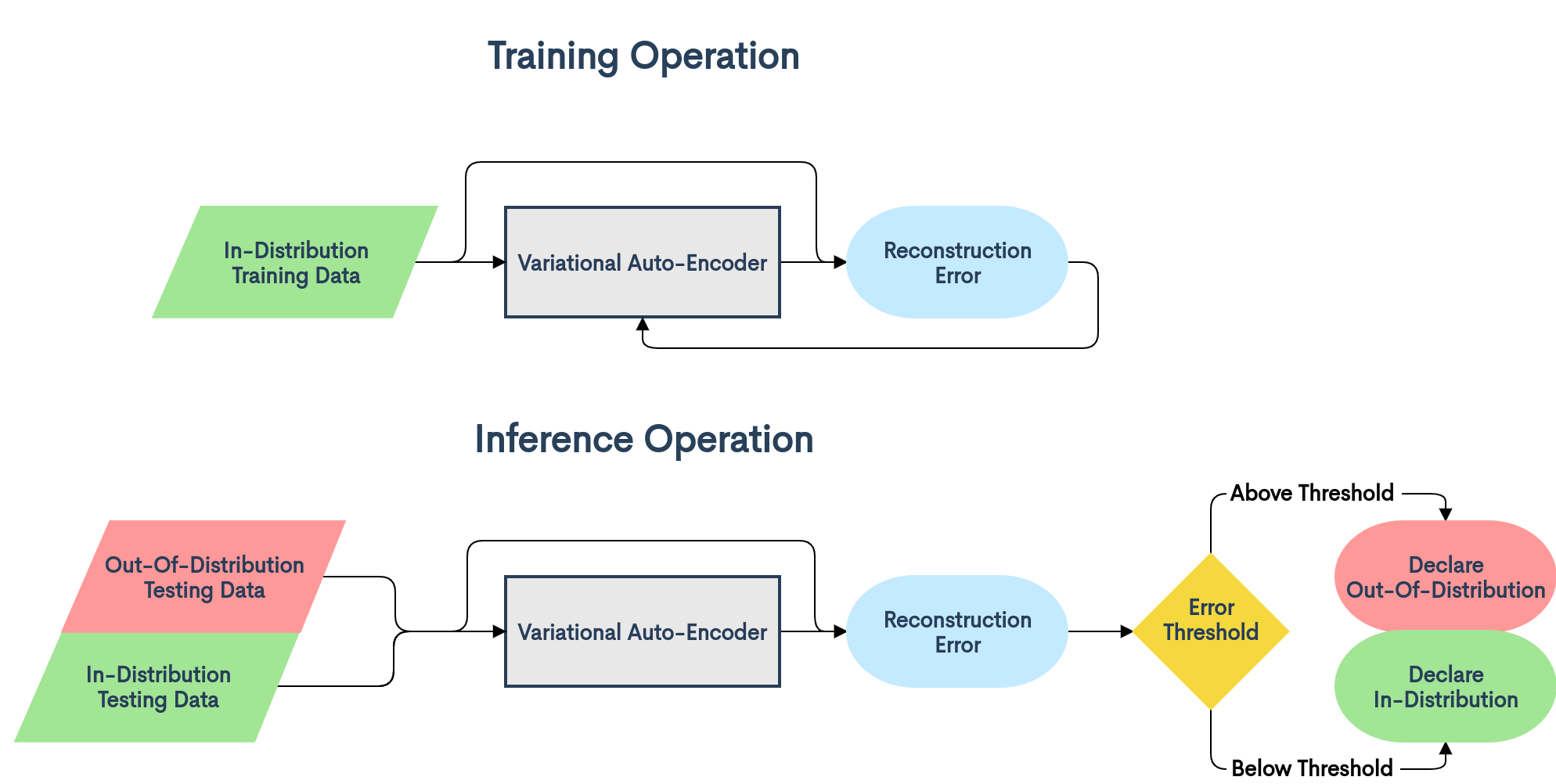
The DOODLER methodology we propose, illustrated in Figure 1, involves training a Variational Auto-Encoder on the same training data as the Deep Learning model you want to perform Out-Of-Distribution Detection for, and then setting conditions on the reconstruction error under which you declare inputs to be OOD. Compared to its closest relatives, ODIN and DAGMM, DOODLER is similarly unsupervised, but improves on DAGMM by being invariant to chip size, improves on ODIN by only requiring one forward pass per input, and improves on them both by enabling image segmentation, illustrating which regions specifically are OOD within an image.
4.1 Variational Auto-Encoder
Per [7], let’s assume that a given sample is generated from a process involving a lower-dimensional latent representation . Where belongs to an high-dimensional field , belongs to a low-dimensional field , such that . If is, say, a three-channel RGB picture of a dog, then , while is a vector in “Dog-Space,” with dimensions describing higher-order concepts like fur length, appearance, posture, and breed.
This allows us to define the process by which becomes , by saying that . In the context of dog photos, would involve taking the vector description of a dog, and using it to produce a picture of the dog described. Furthermore, we might hypothesize that is invertible, with inverse , such that . Here, would start by taking a picture of a dog, and then producing the vector description of that dog, with the condition that this vector can be used by to reconstruct the original image of the dog.
However, while , containing photographs, can be reasonably understood by humans, the field , containing the perfect description of dogs, and the process , by which a dog is brought into existence and photographed, are almost certainly inscrutable. What higher-order concepts might a human overlook when discussing a dog or its appearance? How could they precisely describe the process by which a dog might be drawn? So, and will instead be approximated via a learning algorithm, using with some manually selected as a stand-in for , and a neural network parameterized with of the form . This will allow for the model to be created automatically by training it on data, and together with a second neural network of the form to invent a meaningful version of . In a sense, by training these two neural networks on photographs of dogs, the requirement that means that and will have to learn to produce a meaningful description of a dog’s fur or posture in a higher-order, lower-dimensional setting than a picture, and to then re-draw that picture based on that description, respectively.
By composing and , they can be referred to as a single model, the Variational Auto-Encoder , with . In order to train this combined model , we will use a training dataset , which consists of samples from a distribution over the input field , and then attempt to minimize for some loss or reconstruction error function . To use DOODLER to detect Out-Of-Distribution inputs for an application, would be the same dataset that the application model was trained on - here, it would contain pictures of dogs - and might be something like pixel-wise Mean Squared Error, which we will justify using in the next section. To optimize the parameters of the VAE, an algorithm like Adam Optimizer might be used, denoted as . This training procedure is given by Algorithm 1.
This produces a model that, in some sense, has an understanding of the structure of . If this understanding was not present, then would not be able to encode an input from into a lower dimension and then have successfully reconstruct it, so they must be leveraging context and patterns within the data to compress and recover information. Because the lower dimension of the compressed state means that some information will be lost, the information that is preserved must be capable of being understood in such a way as to fill in most of the missing information. If trained on pictures of dogs, by understanding what dogs look like might encode information like “the tail is at this location, and is upright with long golden-brown fur” in order for to reconstruct the pixel information of the region containing the tail.
However, since this model operates entirely on the basis of understanding the structure of , if it was provided with sampled from somewhere else, possessing structures and patterns that differ greatly from , then it’s reasonable to assume that would be relatively large. For example, if a photograph of an airplane was put into the Variational Auto-Encoder trained on pictures of dogs, we could guess that would not be able to successfully encode the appearance of a jet engine into dimensions like “fur length” and “ear size,” instead producing numerical gibberish. From there, would attempt to turn that gibberish into a picture of some kind of weird dog, resulting in significant error when compared to the original airplane.
4.2 Reconstruction Error
Within the framework of [7], a “canonical” Variational Auto-Encoder consists of two parts, and , which are conditional probability estimators, with being the estimated probability that is the true encoding of , and being the estimated probability of receiving given the encoding . This means that training and involves reducing the degree to which they disagree for any given sample . For example, if is high, meaning estimates that is likely the true encoding of , then should be low everywhere besides . This disagreement over when considering is expressed as the Kullback-Leibler Divergence:
However, actually estimating and its gradients is computationally infeasible. Going forward, we’ll be abbreviating the notation using and , to make further algebraic work more legible. By using the same assumption as [7] that the distributions over represented by and approximate multivariate Gaussian distributions, we get the closed form:111Here, as in standard Statistical notation, is the covariance matrix and is the vector-valued mean of a multivariate distribution. Additionally, ‘’ and ‘’ are the trace and determinant of a matrix, and ‘’ is the dimension of a field.
Next, it’s worth noting that a nonzero covariance between different dimensions in in either distribution would mean that the same information was being stored in multiple entries in . Because the number of entries is very limited, this repetition in storage is expected to disappear, and the covariance matrices will become approximately diagonal. By replacing the covariance matrices with just their diagonal entries in the form of variance vectors , and by removing the constant due to the dimension of , we can approximate and simplify this expression without seriously affecting the future gradients with respect to :
Lastly, we can insert a normalization step into the modeling process itself, forcibly setting the variances along each dimension to 1. This guarantee reduces the entire expression to:
What this means is that, effectively, when given , the gradient behavior of the Kullback-Leibler Divergence between and is similar to that of the distance between their means in . By moving back into thinking in terms of functions, with and , we can use the local continuity of and to get:
Meaning that it’s possible to relate the Kullback-Leibler Divergence over to the Mean Squared Error in , reducing to a loss function given by:
| (1) |
Which satisfies the condition that the value of which minimizes is the same as the mean of given with optimal , or
Therefore, the mean of the squared differences between and has gradient behavior that is approximately equivalent to that of the Kullback–Leibler formulation, and can be used both as a loss function for the direct optimization of the Variational Auto-Encoder for Algorithm 1, and as the reconstruction error during inference.
5 Error Distribution Analyses
In order to find the best rules to use to declare samples to be Out-Of-Distribution, we have to know the probability distributions of the reconstruction errors. As we see in Figure 2222This histogram was produced with 80 samples each from the testing sets of CIFAR-100 and TinyImagenet, using a VAE trained on CIFAR-100. This behavior, with the pixel-wise differences approximating Gaussian distributions, is general between different datasets., the pixel-wise differences between and approximate a Gaussian distribution. As a result, the reconstruction error of an image, given by from Equation 1, being the mean of the squares of values sampled from what is approximately Gaussian, approximates a Gamma distribution.333Formally, a Gamma distribution represents the probability of receiving a given sum when adding the squares of a known number of values sampled from a Gaussian distribution. But, because a mean is the sum over a set divided by its size, and a Gaussian divided by a constant is another Gaussian, the mean of the squares follows a Gamma distribution, the same as their sum. This aligns well with the Gamma distribution-esque appearances of the histograms of image-wise reconstruction errors, as in Figure 6.
Taking the formulation of the Gamma distribution, we can give the probability density function as:
With being the Gamma function. Because the mean and the variance of the Gamma distribution are known to be and respectively, and because the mean and variance of the distribution of can be approximated as and to a high degree of precision with a large enough number of samples, and can be solved for using the Method of Moments:
Given a VAE trained on the training set sampled from , it is now possible to produce a distribution , the probability density of receiving as the reconstruction error if we know that was sampled from the In-Distribution. We do this by taking a test set that has also been sampled from , calculating the mean and variance of over , and then using them to solve for and . Using the same method, but a test set that has been sampled from , we can solve for and , which parameterize , the probability density of when was sampled from Out-Of-Distribution.
5.1 Out-Of-Distribution Sample Detection
| True Positive | and |
|---|---|
| False Positive | and |
| False Negative | and |
| True Negative | and |
If some prior probabilities are assumed, as well as the existence of a relatively small Out-Of-Distribution dataset sampled from to determine , it is possible to use Bayes’ Theorem to compute with
At which point going below some threshold probability would be used to declare a positive Out-Of-Distribution Detection. However, it must be noted that this does rely on both the existence of , and on the approximate equivalence between and . But, these are much weaker assumptions than those made by works like [16], as we’re not using a dataset sampled from for training , reducing the quantity of data needed. We only ever use to approximate the parameters of Statistical distributions, not to capture the actual underlying behavior of .
For a given threshold probability , it’s possible for us to calculate the expected True Positive, False Positive, False Negative, and True Negative proportions of the inferences made. With “positive” meaning the presence of an Out-Of-Distribution sample, these are the proportions of incoming data that were sampled Out-Of-Distribution and correctly detected, that were sampled In-Distribution and incorrectly detected as Out-Of-Distribution, that were sampled Out-Of-Distribution and incorrectly ignored as In-Distribution, and that were sampled In-Distribution and were correctly ignored, respectively.
Under the assumption that , the distribution of reconstruction errors from the Out-Of-Distribution, is shifted to the right of , the distribution from the In-Distribution, this begins by finding the matching threshold value , using:
And then using the conditions from Table 2 to define when a sample will fall into each category. These conditions lead to the formulae listed in Table 3, which can be used to calculate the proportions of the data that will fall into each category. Because those formulae, when applied to this situation, involve integrating the probability density function of the Gamma distribution, it may be useful to replace the integral with the cumulative density function:
But this comes with the caveat that is itself defined as the integral that satisfies this condition, rather than it being possible to reduce the integral to elementary functions. Next, having determined those proportions, we can calculate the Sensitivity, Specificity, Positive Predictive Value, and Negative Predictive Value, using the relationships from Table 4. Those values in turn can be used to produce the Receiver Operating Characteristic () curve. This curve is generated by pairs of the False Positive Rate, or “Fall-Out,” and the True Positive Rate, or “Recall,” taken at the same threshold value. These are not the False Positive Proportion and True Positive Proportion from Tables 2 and 3, but rather the rates at which negative cases are declared positive and positive cases are declared positive, respectively. The False Positive Rate/Fall-Out, here , is the probabilistic inverse of Specificity, and the True Positive Rate/Recall, here , is equivalent to Specificity. These are used to produce the curve:
Which may be turned into a functional form:
And then integrated, to retrieve the Area Under the ROC Curve (AUROC):
This integral itself being possible to approximate computationally by using an interpolation method on a finite subset of to yield . Getting this number, the AUROC, is useful, as it represents the model’s trade-off between the True Positive Rate and the False Positive Rate at different thresholds. A high AUROC means that the model can have both a high True Positive Rate and a low False Positive Rate at the same time, indicating that the model performs well. A similar method can be used to calculate the Area Under the Precision-Recall Curve, which measures how the model trades off between minimizing false positives, and minizing false negatives.
5.2 Out-Of-Distribution Pixel Detection
One of the most important usecases of Out-Of-Distribution Detection involves alerting a human operator that an OOD input has been detected, so that the human can make a more sensible decision than a model would be able to. What might be helpful for a human analyst is to understand what, specifically, about the input caused it to declared OOD. Helpfully, DOODLER can be used to produce a segmentation over an image, based on how likely it is that each individual pixel belongs to an OOD input.
Determining the probability of a given pixel having been sampled OOD based on the reconstruction error falls along similar lines to doing for an entire sample. Collect pixel-wise reconstruction errors from both In-Distribution and Out-Of-Distribution samples, determine the parameters of the distributions that produce them, and then use Bayes’ Theorem again. For a given pixel reconstruction error produced by a pixel :
We can use distributions to approximate and , because they’re the distributions of the squares of values from a single Gaussian. The distribution only has a single parameter, , which is the same as its mean, and a probability density function given by:
5.3 Out-Of-Distribution Stream Detection
Compared to sample detection, stream detection doesn’t even require a dataset or overly restrictive assumptions about , as we can do it entirely through the use of Hypothesis Testing.
For this setting, let’s say that there’s a stream of data from which is being sampled, like a sensor in a new location. Then the reconstruction error for a given sample is the result of comparing the output of the trained model to the sample, . By assuming that the expected error for Out-Of-Distribution samples is greater than it is for In-Distribution samples, the Null Hypothesis, , and the Alternative Hypothesis, , can be taken according to Table 5. Essentially, we start by assuming , that is producing ID data, with low reconstruction errors. Under this assumption, we can calculate the probability that we’d see the mean reconstruction error that has given us so far. If this probability is too low, we can reject , saying that it’s an unreasonable assumption in light of the evidence, and accept , declaring that is sampling from Out-Of-Distribution, because it’s producing higher reconstruction errors.
The Central Limit Theorem gives us that, if we repeatedly take a number of samples from a population and calculate their mean, the distribution of the means over the repetitions approaches a normal distribution, allowing us to use Gosset’s/Student’s -test.444This Statistical test, involving using a test statistic based on the number of standard errors that a sample mean differs from its expectated value if it was produced by a known population, was originally developed by Brewer and Statistician William Sealy Gosset, while working at Guinness. At the time, this new test allowed brewers to draw meaningful conclusions about new strains of barley or Chemical processes from smaller sample sizes. Because use of this new test for brewing constituted a trade secret, and Guinness required their researchers to write under pseudonyms, Gosset published his work under the name “Student,” after which his -test and -distribution are named To start, take a set of samples:
And take the difference between the mean reconstruction error from this set , and the expected reconstruction error from the In-Distribution :
From there, take the standard error of the mean over samples, using the standard deviation of the In-Distribution :
Which lets us calculate the test statistic:
And then we can choose to reject the Null Hypothesis depending on whether or not exceeds the -score, the number of standard errors required to produce this result if the expected mean of the samples was equal to the mean of the population, corresponding to the significance level, or -value.
Under the hypothesis that really was sampling from , we would expect the mean reconstruction error yielded from samples from would follow a normal distribution centered around the expected reconstruction error from . This test statistic then tells us how many standard deviations above the expected reconstruction error the mean reconstruction error of your samples is. By using that number of standard deviations, together with the cumulative density of the normal distribution, we can determine the likelihood of receiving a value for as or more extreme than the one that appeared. If this likelihood is too low, say ¡1%, we reject the Null Hypothesis, and say that something must be increasing the reconstruction errors of the data from , namely, that they’re OOD.
6 Experimentation
FPR at Detection AUPR AUPR ID OOD 95% TPR Error AUROC Out In ODIN/DAGMM/DOODLER MNIST F-MNIST 0.49/0.35/0.19 0.27/0.2/0.12 0.89/0.92/0.96 0.89/0.92/0.96 0.88/0.92/0.96
Following other papers on the subject [1, 12], our experiments were done by selecting two available Computer Vision datasets, and declaring one to be the In-Distribution, and the other Out-Of-Distribution. Then a VAE was trained on the training portion of the ID dataset, and used to classify samples from the testing portions of both the ID and OOD datasets. For example, Table 6 shows an experiment where a VAE was trained on the training portion of the MNIST dataset, and then was tasked with classifying testing MNIST samples as In-Distribution, versus Fashion-MNIST samples as Out-Of-Distribution. The metrics shown will be explained in the Results and Comparisons section.
The datasets we selected include MNIST [11], Fashion-MNIST [21], Omniglot [9], CIFAR-100 [8], TinyImagenet [3, 10], SVHN [17], and CelebA [14]. These datasets were collected together into “simple” and “complex” groups, with MNIST, F-MNIST, and Omniglot in the former, and CIFAR-100, TinyImagenet, SVHN, and CelebA in the latter. Each dataset had its own VAE trained for it, which was then tested with DOODLER for its ability to detect samples from every other dataset in the group as Out-Of-Distribution. Additionally, in both groups, random Gaussian noise clipped to and Uniform noise from were added as purely OOD samples.
Implementations of ODIN and DAGMM were used as comparisons, with models similar in capability and with equivalent training regimens to the VAEs used for DOODLER.
7 Results and Comparisons
FPR at Detection AUPR AUPR ID OOD 95% TPR Error AUROC Out In ODIN/DAGMM/DOODLER MNIST F-MNIST 0.49/0.35/0.19 0.27/0.2/0.12 0.89/0.92/0.96 0.89/0.92/0.96 0.88/0.92/0.96 Omniglot 0.33/0.21/0.07 0.19/0.13/0.06 0.93/0.96/0.98 0.93/0.97/0.98 0.93/0.96/0.98 Gaussian 0.12/0.17/0.01 0.09/0.11/0.03 0.98/0.97/1.0 0.98/0.97/1.0 0.98/0.97/1.0 Uniform 0.12/0.17/0.02 0.08/0.11/0.03 0.98/0.96/1.0 0.98/0.96/1.0 0.98/0.96/0.99 F-MNIST MNIST 0.49/0.23/0.01 0.27/0.14/0.03 0.88/0.95/1.0 0.88/0.95/1.0 0.88/0.95/1.0 Omniglot 0.59/0.18/0.0 0.32/0.12/0.03 0.85/0.97/1.0 0.86/0.97/1.0 0.85/0.96/1.0 Gaussian 0.02/0.02/0.02 0.03/0.04/0.03 0.99/1.0/0.99 0.99/0.99/0.99 0.99/0.99/0.99 Uniform 0.02/0.01/0.03 0.04/0.03/0.04 0.99/1.0/0.99 0.99/1.0/0.99 0.99/1.0/0.99 Omniglot MNIST 0.22/0.43/0.04 0.14/0.24/0.04 0.96/0.89/0.99 0.95/0.9/0.99 0.96/0.89/0.99 F-MNIST 0.26/0.56/0.05 0.16/0.3/0.05 0.94/0.87/0.99 0.95/0.88/0.99 0.94/0.86/0.99 Gaussian 0.03/0.08/0.0 0.04/0.07/0.03 0.99/0.98/1.0 0.99/0.98/1.0 0.99/0.98/1.0 Uniform 0.03/0.06/0.0 0.04/0.05/0.03 0.99/0.99/1.0 0.99/0.99/1.0 0.99/0.99/1.0
FPR at Detection AUPR AUPR ID OOD 95% TPR Error AUROC Out In ODIN/DAGMM/DOODLER CIFAR-100 TinyImagenet 0.81/0.63/0.5 0.43/0.34/0.28 0.73/0.81/0.86 0.73/0.79/0.86 0.71/0.81/0.86 SVHN 0.84/0.93/0.8 0.44/0.49/0.42 0.68/0.57/0.71 0.66/0.55/0.69 0.67/0.55/0.7 CelebA 0.84/0.82/0.47 0.45/0.44/0.26 0.67/0.72/0.88 0.66/0.7/0.88 0.66/0.71/0.88 Gaussian 0.03/0.02/0.01 0.04/0.04/0.03 0.99/1.0/1.0 0.99/0.99/1.0 0.99/0.99/1.0 Uniform 0.02/0.02/0.0 0.04/0.04/0.03 0.99/1.0/1.0 0.99/0.99/1.0 0.99/0.99/1.0 TinyImagenet CIFAR-100 0.89/0.75/0.64 0.47/0.4/0.34 0.62/0.73/0.82 0.61/0.71/0.82 0.61/0.72/0.82 SVHN 0.78/0.79/0.67 0.41/0.42/0.36 0.74/0.74/0.78 0.73/0.74/0.78 0.72/0.73/0.77 CelebA 0.61/0.53/0.78 0.33/0.29/0.41 0.81/0.86/0.72 0.81/0.86/0.71 0.81/0.86/0.72 Gaussian 0.03/0.04/0.01 0.04/0.05/0.03 0.99/0.99/1.0 0.99/0.99/1.0 0.99/0.99/1.0 Uniform 0.03/0.03/0.01 0.04/0.04/0.03 0.99/0.99/1.0 0.99/0.99/1.0 0.99/0.99/1.0 SVHN CIFAR-100 0.58/0.45/0.32 0.32/0.25/0.19 0.85/0.9/0.93 0.86/0.9/0.92 0.84/0.9/0.93 TinyImagenet 0.23/0.41/0.14 0.14/0.23/0.1 0.95/0.91/0.97 0.95/0.91/0.97 0.95/0.91/0.97 CelebA 0.35/0.23/0.06 0.2/0.14/0.05 0.91/0.96/0.99 0.91/0.96/0.99 0.91/0.96/0.99 Gaussian 0.01/0.01/0.01 0.03/0.03/0.03 1.0/1.0/1.0 0.99/0.99/1.0 0.99/0.99/1.0 Uniform 0.02/0.02/0.01 0.03/0.04/0.03 1.0/0.99/1.0 1.0/0.99/1.0 1.0/0.99/1.0 CelebA CIFAR-100 0.86/0.78/0.9 0.46/0.41/0.47 0.67/0.73/0.6 0.67/0.72/0.6 0.65/0.72/0.59 TinyImagenet 0.64/0.54/0.73 0.35/0.29/0.39 0.81/0.85/0.75 0.8/0.84/0.75 0.8/0.85/0.75 SVHN 0.61/0.82/0.89 0.33/0.44/0.47 0.81/0.7/0.61 0.8/0.69/0.6 0.81/0.68/0.61 Gaussian 0.02/0.02/0.01 0.03/0.04/0.03 1.0/1.0/1.0 1.0/0.99/1.0 1.0/0.99/1.0 Uniform 0.02/0.02/0.01 0.03/0.03/0.03 1.0/1.0/1.0 1.0/0.99/1.0 1.0/0.99/1.0
When doing analyses of the results, we assumed the prior probabilities of receiving an In-Distribution and an Out-Of-Distribution sample, respectively, to both be .
The metrics used are taken from [6, 12, 1]. They include:
-
•
The FPR at 95% TPR, which is the probability of an ID sample being accidentally declared OOD when a real OOD sample has a 95% chance of being detected. This should be minimized.
-
•
Detection Error is the over-all probability of any given sample being misclassified when at a 95% True Positive Rate. This should be minimized.
-
•
Area Under the Receiver Operating Characteristic curve is the over-all probability that an OOD sample receives a higher metric than an ID sample, in the case of DOODLER a higher reconstruction error. This should be maximized.
-
•
Area Under the Precision-Recall curve represents balancing a low rate of false positives with a high rate of collecting true positives. Both the AUPR calculated with OOD samples being positive and ID samples being positive are provided. Both should be maximized.
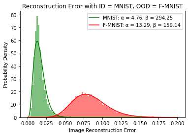
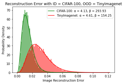
Looking at Tables 7 and 8, we can see that DOODLER competes very well against ODIN and DAGMM, often superseding them. An example of this high performance is seen in the graph of reconstruction errors on MNIST and Fashion-MNIST with a VAE trained for MNIST, given in Figure 3, which highlights the differences between the reconstruction error distributions. In that figure, we see very little overlap, meaning that determining which inputs belong to which dataset based on the reconstruction error yields good results. Similarly, Figure 4 shows the differences in the reconstruction errors between CIFAR-100 and TinyImagenet with a VAE trained on CIFAR-100. While the differences are less stark, they are still very significant, allowing DOODLER to reach an AUROC of 0.86.
Looking at Figures 5 and 6, which contain the distributions regressed from the actual error contributions of individual pixels, shows us that the actual difference between how accurate the VAE is on any given pixel of an In-Distribution versus an Out-Of-Distribution input is relatively subtle. Rather, the large differences in over-all image reconstruction error are due to the small per-pixel differences adding up over a very large number of pixels, producing very different per-image distributions.
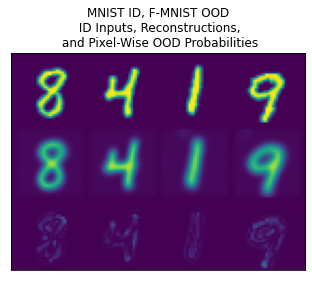
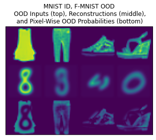
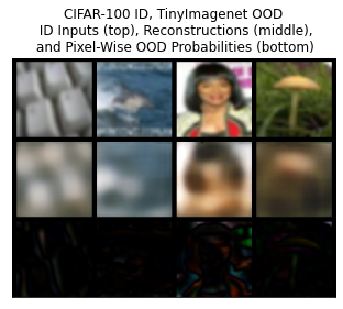
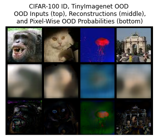
Additionally, Figures 7 and 8 provide examples of inputs, reconstructions, and the estimated per-pixel Out-Of-Distribution likelihoods from both In-Distribution and OOD samples. Even though the reconstructions on the visually complex datasets are quite cloudy, they do align relatively well with the inputs in shape and color on the ID samples, while failing on the OOD samples, producing significantly greater error. Looking at the pixel-wise OOD likelihood estimation, it becomes clear to see that the bright spots align themselves closely with features in the image, representing the objects that the VAE was unfamiliar with from training.
This means that the intuitions developed earlier about the functionality of DOODLER being based on a failure to reconstruct unseen data bear out experimentally, because on a fundamental level, what is happening is that the VAEs trained on the In-Distribution are failing to reconstruct objects they haven’t seen before in the Out-Of-Distribution inputs. In a very real sense, this means that DOODLER is performing Out-Of-Distribution Detection to the letter, because it highlights objects that don’t exist within the In-Distribution.
8 Conclusions and Future Work
While DOODLER represents a step forward for Out-Of-Distribution detection, work remains to be done. This includes placing theoretical bounds on its error rate, understanding the reconstruction error distributions more wholly than is possible with Gamma distributions, and increasing the saliency of pixel-wise segmentations. Additionally, it might be worthwhile to try and study the connection between how the Variational Auto-Encoder builds its latent space, and the resulting reconstruction errors, to help establish what exactly in the sample has resulted in detection as an OOD input. It might also be worthwhile to pair the VAE with some kind of Generative Adversarial framework [4], to try and improve the sharpness of the reconstructions. It may also be possible to further improve on OOD Detection by combining elements from multiple methodologies, including DOODLER, or by using a an ensemble of them to cover each other’s weaknesses.
There is also work to be done to study how DOODLER behaves when provided with adversarial inputs. For example, can an adversarial attack actually decrease the reconstruction error of an input? This could be a potential avenue of attack, if an adversary wanted to provide an anomalous input without a human operator being notified.
But, to conclude, DOODLER represents a novel framework for Out-Of-Distribution Detection, introducing a functional perspective to the problem, improving on aspects of earlier methods, and providing a basis on which to pursue functionality like image segmentation. This constitutes a step forwards in the pursuit of making Machine Learning robust and trustworthy for real-world applications.
References
- [1] Vahdat Abdelzad, Krzysztof Czarnecki, Rick Salay, Taylor Denouden, Sachin Vernekar, and Buu Phan. Detecting out-of-distribution inputs in deep neural networks using an early-layer output. CoRR, abs/1910.10307, 2019.
- [2] Petra Bevandić, Ivan Krešo, Marin Oršić, and Siniša Šegvić. Discriminative out-of-distribution detection for semantic segmentation. arXiv preprint arXiv:1808.07703, 2018.
- [3] Jia Deng, Wei Dong, Richard Socher, Li-Jia Li, Kai Li, and Li Fei-Fei. Imagenet: A large-scale hierarchical image database. In 2009 IEEE conference on computer vision and pattern recognition, pages 248–255. Ieee, 2009.
- [4] Ian Goodfellow, Jean Pouget-Abadie, Mehdi Mirza, Bing Xu, David Warde-Farley, Sherjil Ozair, Aaron Courville, and Yoshua Bengio. Generative adversarial nets. Advances in neural information processing systems, 27, 2014.
- [5] Dan Hendrycks, Steven Basart, Mantas Mazeika, Mohammadreza Mostajabi, Jacob Steinhardt, and Dawn Song. A benchmark for anomaly segmentation. arXiv preprint arXiv:1911.11132, 2019.
- [6] Dan Hendrycks and Kevin Gimpel. A baseline for detecting misclassified and out-of-distribution examples in neural networks. CoRR, abs/1610.02136, 2016.
- [7] Diederik P Kingma and Max Welling. Auto-encoding variational bayes, 2014.
- [8] Alex Krizhevsky, Vinod Nair, and Geoffrey Hinton. Cifar-100 (canadian institute for advanced research).
- [9] Brenden M. Lake, Ruslan Salakhutdinov, and Joshua B. Tenenbaum. Human-level concept learning through probabilistic program induction. Science, 350(6266):1332–1338, 2015.
- [10] Ya Le and X. Yang. Tiny imagenet visual recognition challenge. 2015.
- [11] Yann LeCun and Corinna Cortes. MNIST handwritten digit database. 2010.
- [12] Shiyu Liang, Yixuan Li, and R. Srikant. Principled detection of out-of-distribution examples in neural networks. CoRR, abs/1706.02690, 2017.
- [13] Shiyu Liang, Yixuan Li, and R. Srikant. Enhancing the reliability of out-of-distribution image detection in neural networks, 2020.
- [14] Ziwei Liu, Ping Luo, Xiaogang Wang, and Xiaoou Tang. Deep learning face attributes in the wild. In Proceedings of International Conference on Computer Vision (ICCV), December 2015.
- [15] Alexander Meinke, Julian Bitterwolf, and Matthias Hein. Provably robust detection of out-of-distribution data (almost) for free. arXiv preprint arXiv:2106.04260, 2021.
- [16] Alexander Meinke and Matthias Hein. Towards neural networks that provably know when they don’t know. arXiv preprint arXiv:1909.12180, 2019.
- [17] Yuval Netzer, Tao Wang, Adam Coates, Alessandro Bissacco, Bo Wu, and Andrew Y Ng. Reading digits in natural images with unsupervised feature learning. 2011.
- [18] Tomaso Poggio, Hrushikesh Mhaskar, Lorenzo Rosasco, Brando Miranda, and Qianli Liao. Why and when can deep-but not shallow-networks avoid the curse of dimensionality: a review. International Journal of Automation and Computing, 14(5):503–519, 2017.
- [19] Doyen Sahoo, Quang Pham, Jing Lu, and Steven CH Hoi. Online deep learning: Learning deep neural networks on the fly. arXiv preprint arXiv:1711.03705, 2017.
- [20] David Williams, Matthew Gadd, Daniele De Martini, and Paul Newman. Fool me once: Robust selective segmentation via out-of-distribution detection with contrastive learning. arXiv preprint arXiv:2103.00869, 2021.
- [21] Han Xiao, Kashif Rasul, and Roland Vollgraf. Fashion-mnist: a novel image dataset for benchmarking machine learning algorithms. CoRR, abs/1708.07747, 2017.
- [22] Marvin Zhang, Henrik Marklund, Nikita Dhawan, Abhishek Gupta, Sergey Levine, and Chelsea Finn. Adaptive risk minimization: A meta-learning approach for tackling group distribution shift. arXiv preprint arXiv:2007.02931, 2020.
- [23] Kaiyang Zhou, Ziwei Liu, Yu Qiao, Tao Xiang, and Chen Change Loy. Domain generalization: A survey. arXiv preprint arXiv:2103.02503, 2021.
- [24] Bo Zong, Qi Song, Martin Renqiang Min, Wei Cheng, Cristian Lumezanu, Daeki Cho, and Haifeng Chen. Deep autoencoding gaussian mixture model for unsupervised anomaly detection. In International Conference on Learning Representations, 2018.
9 Example Figures