Rotation and deformation of strangeon stars in the Lennard-Jones model

Abstract

The strong interactions at low energy scales determine the state of the supranuclear matter in the pulsar-like compact objects. It is proposed that the bulk strong matter could be composed of strangeons, which are quark clusters with a nearly equal number of three light-flavor quarks. In this work, to characterize the strong-repulsive interactions at short distances and the non-relativistic nature of the strangeons, the Lennard-Jones model is used to describe the equation of state (EoS) of strangeon stars (SSs). We investigate the static, the slowly rotating, and the tidally deformed SSs in detail. The corrections resulted from the finite surface densities are considered crucially in the perturbative approaches. We also study the universal relations between the moments of inertia, the tidal deformabilities, and the quadrupole moments. Those results are ready to be used for various purposes in astrophysics, and possible constraints from contemporary observations on the parameter space of the Lennard-Jones model are discussed. Future observations of the pulsars’ radio signals, the X-ray emissions from the hot spots on the surface of the stars, and the gravitational waves (GWs) from binary mergers can give tighter constraints or even verify or falsify the existence of SSs.

1 Introduction

The equation of state (EoS) of the supranuclear matter in pulsar-like compact stars remains unknown. Traditionally, people believe that neutron stars (NSs) are formed in the supernova explosions. However, there is another possibility that the energetic electrons in the collapsed stellar core are eliminated by transforming the $u/d$ quarks to the $s$ quark. Witten (1984) conjectured that the pulsar-like compact objects should be quark stars (QSs), which contain strange quark matter (SQM) with nearly equal number of $u$, $d$, $s$ quarks, and a small fraction of electrons to keep the neutrality. Some efforts have been made to understand the state of pulsar-like compact stars in the framework of conventional QSs, including the MIT bag model with almost free quarks (Alcock et al., 1986) and the color-superconducting state model (Alford et al., 2008).

Realistic densities inside pulsar-like compact stars ($\rho\sim 2-10\,\rho_{0}$ where $\rho_{0}$ is the saturation density of nuclear matter) are not high enough to justify the validity of perturbative quantum chromodynamics (QCD). The perturbative QCD, based on asymptotic freedom, works well only at high energy scales, $E_{\rm scale}\gtrsim 1$ GeV. However, the state of pressure-free strong matter at supranuclear density pertains to non-perturbative QCD because $E_{\rm scale}\lesssim 1$ GeV, analogous to the case of normal atomic nuclei. In addition, the difficulties to obtain the relativistic EoS of cold quark matter at several nuclear densities also come from the fact that the vast assemblies of interacting particles face the complicated quantum many-body problem (Xu, 2009, 2018; Alford et al., 2008; Baym et al., 2018). The uncertainty in EoS introduces additional uncertainty to the strong-field gravity tests as well (Shao et al., 2017; Shao, 2019).

It is phenomenologically conjectured that, in cold matter at supranuclear density, the constituent units could be strange quark clusters (Xu, 2003), since the strong interaction may render quarks grouped in quark-clusters. Each quark-cluster is composed of several quarks (including $u$, $d$ and $s$ quarks) condensing in position space rather than in momentum space. A strange quark cluster is named “strangeon,” being coined to “strange nucleon” (Xu & Guo, 2017; Lai & Xu, 2017). The astrophysically compressed baryonic matter, therefore, should be in a state of strangeon matter, and pulsar-like compact stars could be strangeon stars (SSs). Moreover, at realistic baryon densities of compact stars, the residual interaction between strangeons could be stronger than their kinetic energy, so strangeons would be trapped in the potential well and the bulk of the dense matter in the compact stars are crystallized into a solid state (Xu, 2003, 2009).

Although the state of bulk strong matter is essentially a non-perturbative QCD problem and is difficult to answer from first principles, the astrophysical point of view could give some hints that bulk strong matter could be in the form of strangeon matter. Strangeon matter may constitute the true ground state of strongly-interacting matter rather than ⁵⁶Fe and neutron matter, and this could be seen as a generalized Witten’s conjecture, while the traditional Witten’s conjecture focuses on the matter composed of almost free $u$, $d$ and $s$ quarks.

Strangeon matter, similar to strange quark matter, is composed of nearly equal numbers of $u$, $d$ and $s$ quarks; however, different from that in strange quark matter, quarks in strangeon matter are localized inside strangeons due to the strong coupling between quarks. There are differences and similarities between SSs and NSs/QSs. On the one hand, quarks are thought to be localized in strangeons in SSs, like neutrons in NSs, but a strangeon has three flavors and may contain more than three valence quarks. The matter at the surface of SSs is still strangeon matter, i.e., SSs are self-bound by strong force, like QSs.

Eventually the theoretical models, including NSs, QSs and SSs, need to be tested by the astrophysical observations. The model of SSs has been found to be helpful to understand different manifestations of pulsar-like compact stars. SSs had been found to be massive (Lai & Xu, 2009a, b) before the discovery of pulsars with $M>2M_{\odot}$ (Demorest et al., 2010). The surface of SSs could naturally explain the pulsar magnetospheric activity (Xu et al., 1999) as well as the subpulse-drifting of radio pulsars (Lu et al., 2019). Starquakes of solid SSs could induce glitches (Zhou et al., 2004, 2014; Lai et al., 2018b) and explain the glitch activity of normal radio pulsars (Wang et al., 2020). The plasma atmosphere of SSs can reproduce the Optical/UV excess observed in X-ray dim isolated NSs (Wang et al., 2017). The tidal deformability (Lai et al., 2019) as well as the light curve (Lai et al., 2018a, 2020) of merging binary SSs are consistent with the results of gravitational wave (GW) event GW170817 (Abbott et al., 2017) and its multiwavelength electromagnetic counterparts (Kasliwal et al., 2017; Kasen et al., 2017).

Some phenomenological models have been applied to investigate the EoS of SSs (Lai & Xu, 2009a, b), which may indicate some properties of QCD at low energy scales and have implications on possible astronomical observations that can give constraints on such models. The strangeons are colorless, just like the molecules are neutral in the bulk of inert gas. Lai & Xu (2009b) utilized the Lennard-Jones model (Jones, 1924) that describes inert gas to characterize the interactions between strangeons. This model well characterizes the non-relativistic nature and the strong-repulsive interactions at short distances. In this work we use this model as the EoS and span a wide range of parameter space to investigate the global properties of SSs. We model the static SSs and compare the structures with that of Tolman IV and Tolman VII solutions (Tolman, 1939; Lattimer & Prakash, 2005).

Astrophysically, pulsars have spins and the rotation will affect the structures of the stars and the spacetime itself. Hartle (1967) and Hartle & Thorne (1968) gave a perturbative approach to describe slowly rotating relativistic stars to the second order of angular frequency $\Omega$. Later, Hartle (1973) developed this formalism to the third order of $\Omega$ and calculated the variations of moments of inertia for distorted NSs. One can evaluate the change of physical quantities at each order of $\Omega$ and investigate various properties of the relativistic stars (Chandrasekhar & Miller, 1974; Weber & Glendenning, 1991; Lattimer & Prakash, 2001; Benhar et al., 2005; Urbanec et al., 2013; Yagi & Yunes, 2013a, b). Remarkably, It has been shown that this perturbative approach can be applied with great accuracy for most observed NSs, even for most millisecond pulsars (Berti & Stergioulas, 2004; Berti et al., 2005; Benhar et al., 2005). In some models of NSs, the relative errors compared to the results obtained by numerical relativity for most quantities are less than $2\%$ if the spin frequency is less than $\sim 600\,\rm Hz$  (Benhar et al., 2005; Berti & Stergioulas, 2004; Berti et al., 2005).

In this work, we use the Hartle-Thorne approximation to study the rotating SSs to the third order of $\Omega$. The match conditions at the boundary of the star which are resulted from the finite surface density are crucially considered. We present systematic results for the moments of inertia, the quadrupole moments, the eccentricities, changes in the gravitational and baryonic masses, and universal relations between some of these quantities. The measurement of the moment of inertia from Lense-Thirring precession can give us constraints on the parameter space of SSs. The other physical quantities and the universal relations are ready to be used to interpret astrophysical observations, such as the light curves of X-ray hot spots on the surface of SSs and GWs from binary SS mergers.

For coalescing binary compact stars, the finite size of the stars at the end of inspiral can not be ignored. Each star is deformed in the tidal field of the companion. The energy goes to deform the star and the tidal induced quadrupole moments will contribute to the GW phasing (Hinderer, 2008; Damour & Nagar, 2009; Dietrich et al., 2021). The phase evolution of the GWs will be faster compared to non-spinning stars with the same component masses. The GW170817 event gives the first constraint on the tidal deformability of NSs (Abbott et al., 2017, 2018, 2019). In this paper, we study the tidal properties of SSs based on the work in Lai et al. (2019) and use the posterior from LIGO/Virgo collaborations to put constraints on the parameter space of the Lennard-Jones model.

Yagi & Yunes (2013a, b) found a remarkable universal relation between the moments of inertia, the tidal deformabilities, and the spin induced quadrupole moments, also known as I-Love-Q relation. The relation is nearly EoS independent and the relative errors can be less than $1\%$ for various EoS models, including NSs and QSs. Based on our calculations of rotation and tidal deformation, we find that SSs in the Lennard-Jones model also satisfy the I-Love-Q relation.

The organization of the paper is as follows. In Sec. 2, we introduce the Lennard-Jones model of SSs. The structures of static SSs are discussed in Sec. 3. Based on the background solutions, in Sec. 4, we investigate the global properties of rotating SSs in the Hartle-Thorne approximation. In Sec. 5, we calculate the tidal deformabilities of SSs and discuss the constraints on the parameter space in our model. Then we study the universal relations between the moment of inertia, the tidal deformability, and the quadrupole moment for SSs in Sec. 6. Finally, we summarize our work in Sec. 7. The ordinary differential equations that determine the structures of slowly rotating relativistic stars are given in Sec. A.

Throughout this paper, we use the geometric units where $G=c=1$. The convention of the metric is $(-,+,+,+)$.

2 Strangeon stars in the Lennard-Jones model

In the Lennar-Jones model (Jones, 1924), the potential between two strangeons is (Lai & Xu, 2009b),

$$u(r)=4\epsilon\left[\left(\frac{\sigma}{r}\right)^{12}-\left(\frac{\sigma}{r}\right)^{6}\right]\,,$$ (1)

where $\epsilon$ is the depth of the potential well, $r$ is the distance between two strangeons, and $\sigma$ is the distance when $u(r)=0$. Though simple, this model has the properties of long-range attraction and short-range repulsion. Note that the $\sigma$-$\omega$ model, which is commonly used to describe the interactions between nucleons, can also be well described by long-range attraction and short-range repulsion (Walecka, 1974). The lattice simulations of QCD indicate a short-distance repulsion (Ishii et al., 2007; Wilczek, 2007). Moreover, the repulsive hardcore is essential to generate a stiff EoS for dense matter constituted of strangeons and plays a fundamental role in determining the structures of SSs.

We take simple cubic lattice structures and ignore the surface tension. The potential energy density is (Lai & Xu, 2009b)

$$\rho_{\rm P}=2\epsilon\left(A_{12}\sigma^{12}n^{5}-A_{6}\sigma^{6}n^{3}\right)\,,$$ (2)

where $A_{12}=6.2$, $A_{6}=8.4$, and $n$ is the number density of strangeons. The lattice of strangeons may form other structures in reality, but the differences should be small and do not affect the structures of SSs significantly. The energy density should also include the rest energy of strangeons, $\rho_{\rm r}$, the kinetic energy from lattice vibrations, $\rho_{\rm L}$, and the kinetic energy from electrons, $\rho_{\rm e}$.

The rest energy of a strangeon is $N_{\rm q}m_{\rm q}c^{2}$, where $m_{\rm q}$ is the mass of a quark and $N_{\rm q}$ is the number of quarks in a strangeon. We take the mass of quarks to be $m_{\rm q}=300\,\rm MeV$, which is about one third of the nucleon’s mass. The parameter $N_{\rm q}$ is not known and we leave it as a free parameter. In the calculations, we take $N_{\rm q}=18$ and $N_{\rm q}=9$. A strangeon with 18 quarks is called quark-alpha (Michel, 1991), which is completely symmetric in spin, flavor, and color spaces.

The vibration energy can be obtained by using the Debye approximation of lattice. The vibrations of the cubic lattice can be decomposed into $3N$ independent oscillation modes (Lai & Xu, 2009b) and the vibration energy density $\rho_{\mathrm{L}}=9(6\pi^{2})^{1/3}\hbar vn^{4/3}/8$, where $v$ is the speed of sound waves. Compared to the sum of potential energy and rest energy, the lattice vibration energy is small even if one assumes $v$ is equal to the speed of light (Lai & Xu, 2009b). For this reason, we ignore the contribution of lattice vibration energy in our calculations.

A small fraction of electrons is needed to keep the equilibrium of chemical potential (Witten, 1984; Alcock et al., 1986). In the MIT bag model of SQM, electrons per baryon are determined by the mass of strange quarks $m_{\rm s}$ and the coupling constant $\alpha_{\rm s}$ between quarks (Farhi & Jaffe, 1984). If one fixes the mass $m_{\rm s}$ of the strange quarks, a larger coupling constant $\alpha_{\rm s}$ will lead to a larger fraction of electrons per baryon. When $\alpha_{\rm s}$ equals 0.3, the number of electrons per baryon is smaller than $10^{-4}$ (Farhi & Jaffe, 1984; Lai & Xu, 2009a, b). In the case of strangeons, we have applied the strong interactions between strangeons. The number density of electrons should be small despite the concrete number is still not clear. Even if we take $10^{-4}$, the Fermi energy of electrons still can be ignored compared to the contribution of potential energy and rest-mass energy of strangeons (Lai & Xu, 2009b; Lai et al., 2019).

The total energy density of the zero temperature dense matter composed of strangeons reads

$$\rho=2\epsilon\left(A_{12}\sigma^{12}n^{5}-A_{6}\sigma^{6}n^{3}\right)+nN_{\rm q}m_{\rm q}c^{2}\,.$$ (3)

From the first law of thermodynamics, one derives the pressure

$$P=n^{2}\frac{\mathrm{d}(\rho/n)}{\mathrm{d}n}=4\epsilon\left(2A_{12}\sigma^{12}n^{5}-A_{6}\sigma^{6}n^{3}\right)\,.$$ (4)

At the surface of the SSs, the pressure becomes zero and we obtain the surface number density of strangeons as $\big{(}A_{6}/(2A_{12}\sigma^{6})\big{)}^{1/2}$. For convenience, we transform it to the number density of baryons

$$n_{\rm s}=\left(\frac{A_{6}}{2A_{12}}\right)^{1/2}\frac{N_{\rm q}}{3\sigma^{3}}\,.$$ (5)

For a given number of quarks $N_{\rm q}$ in a strangeon, the EoS of SSs is completely determined by the depth of the potential $\epsilon$ and the number density of baryons $n_{\rm s}$ at the surface of the star. The nucleon-nucleon scattering data indicate that the internucleon potential well lies in the range of $\sim$ $50$–$120$$\,\rm MeV$ for the ${}^{1}S_{0}$ (spin singlet and $s$-wave) channel  (Wiringa et al., 1995; Stoks et al., 1994; Machleidt, 2001); see Fig. 1 of Ishii et al. (2007). Since the strong interactions are not sensitive to the flavor of quarks, we choose $\epsilon$ spanning in the range of $20$–$100\,\rm MeV$, which is similar to the internucleon potential and enough to trap the strangeons in the potential well. The surface baryonic density $n_{\rm s}$ should be in the same order as the nuclear saturation density, $n_{0}=0.16\,\rm fm^{-3}$. But unlike proton or neutron with 3 quarks, we take $N_{\rm q}$ to be 9 or 18 for strangeons. The interactions may group the quarks more compactly compared to nuclei with the same number of quarks. Therefore, we let $n_{\rm s}$ lie in the range of $0.24\,\rm fm^{-3}$ to $0.36\,\rm fm^{-3}$, which corresponds to $1.5\,n_{0}$ to $2.25$$\,n_{0}$.

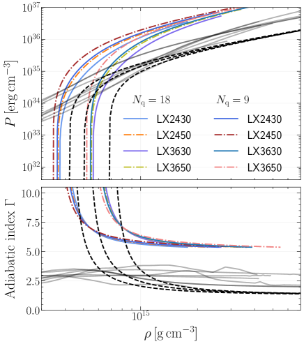
Figure 1: The upper panel shows the relation between mass–energy density $\rho$ and pressure $P$. The Lennard-Jones models of SSs with different choices of the potential depth $\epsilon$, the surface number density of baryons $n_{\rm s}$, and the number of quarks in a strangeon $N_{\rm q}$ are displayed. For comparison, we also show the EoS models of normal NSs (grey) and QSs (black). Correspondingly, the lower panel shows the adiabatic index $\Gamma$ for SSs (colored), normal NSs (grey), and QSs (black). We name EoS of SSs according to different combinations of $n_{\rm s}$ and $\epsilon$. For example, “LX2450” means the surface baryon number density $n_{\rm s}=0.24\,\rm fm^{-3}$ and the potential depth $\epsilon=50\,\rm{MeV}$.

In the upper panel of Fig. 1, we show the EoS of SSs for $N_{\rm q}=18$ and $N_{\rm q}=9$. Different surface densities and potential depths are chosen. We also present the EoS of normal NSs and QSs (Lattimer & Prakash, 2001; Lackey et al., 2006), including the models for normal NSs and SQMs for QSs. Compared to normal NS models, the surface densities of SSs and QSs are not zero and in the order of nuclear density, which originate from the fact that SSs and QSs are self-bound systems while normal NSs are gravitational-bound systems.

One can surely neglect the entropy gradient for the zero temperature EoS of SSs. Therefore, the increases in pressure and density toward the center of the star are adiabatic (Shapiro & Teukolsky, 1983). The adiabatic index $\Gamma$ is defined as

$$\Gamma=\frac{n}{P}\frac{{\rm d}P}{{\rm d}n}=\frac{\rho+P}{P}\frac{\partial P}{\partial\rho}\,,$$ (6)

which determines the change of pressure $P$ associated with the variations of the local density $n$ of particles (Shapiro & Teukolsky, 1983). For relativistic stars in equilibrium, the adiabatic index $\Gamma$ measures the stiffness of the EoS. In the lower panel of Fig. 1, we show the relation between the adiabatic index $\Gamma$ and the mass-energy density $\rho$. One notices that the adiabatic index for SSs is larger than that of NSs, which indicates that SSs are stiffer than normal NSs. The adiabatic index for QSs has the same trend as the SSs. But it becomes much smaller than that of SSs at high densities. The EoS of QSs is taken as $P=(\rho-4B)/3$, where $B$ is the bag constant. At low densities, $\Gamma$ goes up since the bag constant is very large. But as the densities increase, the free quarks in QSs become relativistic and the EoS is softened. For SSs, the repulsive hardcore and the non-relativistic nature of the particles make the EoS always be stiff.

One main concern of the Lennard-Jones model for SSs is that the adiabatic sound speed $c_{\rm s}=(\partial P/\partial\rho)^{1/2}$ turns into superluminal in high pressure. The possibility that the adiabatic sound speed $c_{\rm s}$ in ultra-dense matter exceeds the speed of light has been discussed in some literature (Bludman & Ruderman, 1968; Ruderman, 1968; Caporaso & Brecher, 1979, 1983; Ellis et al., 2007). The central question is: what does $\partial P/\partial\rho$ mean for a relativistic fluid? The expression $\partial P/\partial\rho$ is borrowed from Newtonian hydrodynamics and comes from a static calculation of the EoS $P=P(\rho)$ by ignoring the dynamics of the medium (Lai & Xu, 2009b). One assumes the infinite speed of interactions and finite temperature. The static sound speed $(\partial P/\partial\rho)^{1/2}$ agrees with the dynamical one. However, for relativistic ultra-dense matter, if one assumes zero temperature and finite speed of the interactions between particles, the adiabatic sound speed is no longer a dynamically meaningful speed of the disturbances, but only a measurement of local stiffness (Caporaso & Brecher, 1983; Lai & Xu, 2009b). From the underlying microscopic picture, Bludman & Ruderman (1968) and Caporaso & Brecher (1979) gave dynamical calculations that particles in dense matter interacting with one another by retarded fields. They found that the propagating sound waves always have a speed less than or equal to the speed of light although $\partial P/\partial\rho>1$.

For SSs, the bulk of the stars are in a solid state and strangeons form lattice. Inspired by Bludman & Ruderman (1968) and Caporaso & Brecher (1979), Lu et al. (2018) carried out a 1$-$dimensional chain model to calculate the dynamical speed of the sound waves in SSs. They found that the causality condition is always satisfied although $(\partial P/\partial\rho)^{1/2}$ can be larger than the speed of light. The ultra stiffness and the violation of commonly used causality limit can lead to many interesting global properties of SSs. Interested readers are referred to the above literature for details.

3 Equilibrium background of spherical and static stars

The line element of an isolated and non-spinning relativistic star can be written as

$${\rm d}s^{2}=g_{\alpha\beta}{\rm d}x^{\alpha}{\rm d}x^{\beta}=-e^{\nu}{\rm d}t^{2}+e^{\lambda}{\rm d}r^{2}+r^{2}\left({\rm d}\theta^{2}+\sin^{2}\theta{\rm d}\phi^{2}\right)\,,$$ (7)

where $\nu$ and $\lambda$ are functions of $r$. Since the star is static, we take the four-velocity $u^{\alpha}$ as

$$u^{t}=e^{-\nu/2},\quad u^{i}=0\,,\quad\quad\left(i=r\,,\theta\,,\phi\right)\,.$$ (8)

We approximate the stress-energy tensor of SSs as perfect fluid,

$$T_{\alpha\beta}=(\rho+P)u_{\alpha}u_{\beta}+Pg_{\alpha\beta}\,,$$ (9)

where $\rho$ and $P$ are the energy density and the pressure. By taking $e^{\lambda}=1/(1-2m/r)$ and substituting Eq. (7) and Eq. (9) in the Einstein equations, one obtains the Tolman-Oppenheimmer-Volkoff (TOV) equations for spherical and static relativistic stars,

$$\frac{{\rm d}m}{{\rm d}r}=4\pi r^{2}\rho\,,$$ (10)

$$\frac{{\rm d}\nu}{{\rm d}r}=\frac{2(m+4\pi r^{3}P)}{r(r-2m)}\,,$$ (11)

$$\frac{{\rm d}P}{{\rm d}r}=-\frac{(\rho+P)\left(m+4\pi r^{3}P\right)}{r(r-2m)}\,,$$ (12)

where $m$ is the gravitational mass enclosed in radius $r$. Integrating Eqs. (10–12) with the boundary conditions at the center of the star,

$$m(r)\mid_{r=0}=0\,,\quad\nu(r)\mid_{r=0}=\nu_{\rm c}\,,\quad P(r)\mid_{r=0}={P}_{\rm c}\,,$$ (13)

and the EoS of SSs in Eqs. (3–4), one obtains the stellar structures of isolated and non-spinning SSs. Here $P_{\rm c}$ is the pressure at the center of the star. The constant $\nu_{\rm c}$ can be determined by matching the interior and exterior solutions at the boundary of the star.

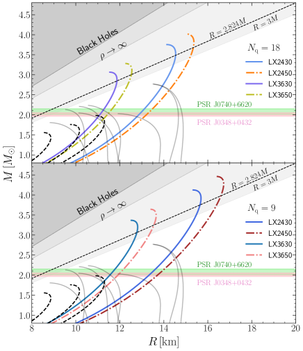
Figure 2: Mass radius relations of SSs for $N_{\rm q}=18$ (upper panel) and $N_{\rm q}=9$ (lower panel) with different combinations of the surface baryonic density $n_{\rm s}$ and the potential depth $\epsilon$. For comparison, we also show the mass radius relations for normal NSs (grey) and QSs (black). The black hole limit ($R=2M$), the limit for the central density to be infinite ($R=9M/4$), the limit for ${\rm d}P/{\rm d}\rho=1$ ($R=2.824M$), the photon spheres ($R=3M$), and the $1$-$\sigma$ region of the mass measurements of PSR J0348+0432 (Antoniadis et al., 2013) and PSR J0740$+$6620 (Fonseca et al., 2021) are illustrated.

In Fig. 2, we display the mass-radius relations of SSs with different choices of $N_{\rm q}$, $n_{\rm s}$, and $\epsilon$. Because the EoS of SSs in the Lennard-Jones model is quite stiff and the maximal mass of SSs can be over $3M_{\odot}$ for large parameter space (Xu, 2018; Lu et al., 2018). The discoveries of massive pulsars, PSR J0348+0432 (Antoniadis et al., 2013) and PSR J0740$+$6620 (Fonseca et al., 2021), at $\sim 2\,M_{\odot}$ via pulsar timing support the stiffness property and more massive ones (e.g., $\geq 2.5\,M_{\odot}$) are expected for our model.

SSs are self-bounded by strong interactions. The trend of the mass-radius relation is basically the same as that of QSs. We can understand it with the help of the adiabatic index $\Gamma$ shown in the lower panel of Fig. 1. At low densities, $\Gamma\rightarrow\infty$ and the gravitational field is weak, which leads to $R\propto M^{1/3}$. As the central densities become larger, the GR effect becomes dominant and it results in the formation of a maximal mass. For QSs, the quarks are nearly free and the interactions are added in a perturbative way. As the central density increases, the quarks become more and more relativistic and the EoS is softened with $\Gamma\rightarrow 4/3$. Therefore, the maximal mass can hardly reach $2\,M_{\odot}$ (Lattimer & Prakash, 2001). While for SSs, the quarks are grouped into non-relativistic clusters and the interactions between strangeons are non-perturbative. We conjecture that the hardcore exists for strangeons just like that for nuclei (Ishii et al., 2007; Wilczek, 2007), and use the Lennard-Jones model to characterize this important feature. The hardcore will make the EoS very stiff. The adiabatic index $\Gamma$ is much larger than QSs at high densities (see Fig. 1). Therefore, the maximal mass $\gtrsim 3\,M_{\odot}$ is possible.

The detailed behaviors of the mass-radius relations for different choices of parameters can be basically understood as follows. For given $n_{\rm s}$, a smaller $N_{\rm q}$ means that the distance $\sigma$ should be smaller according to Eq. (5). Compared to the case of $N_{\rm q}=18$, the adiabatic index $\Gamma$ for $N_{\rm q}=9$ is larger and the EoS is stiffer. Consequently, for given $n_{\rm s}$ and $\epsilon$, the radius at given mass and the maximal mass are larger for $N_{\rm q}=9$. If $N_{\rm q}$ is fixed, the parameters $n_{\rm s}$ and $\epsilon$ completely determine the EoS. Both the increase of the potential depth $\epsilon$ and the decrease of surface density $n_{s}$ make a stiffer EoS since the repulsive force is amplified. For example, the LX2430 is softer than LX2450, but stiffer than LX3630.

Another important feature is that the mass-radius relations of SSs can invade into the commonly used causality limit $R=2.824M$ (Lattimer, 2012). This limit assumes that the EoS has a single parameter $\rho_{0}$ and satisfies the relation $P=0$ for $\rho<\rho_{0}$ and $P=\rho-\rho_{0}$ for $\rho\geq\rho_{0}$. Integrating TOV equations with this EoS, one obtains the maximal mass of NSs to be $M_{\rm max}\simeq 4.09(\rho_{\rm s}/\rho_{0})^{1/2}M_{\odot}$ (Lattimer, 2012), where $\rho_{\rm s}$ is the nuclear saturation density. If one knowns the EoS approximately up to $2\rho_{\rm s}$, the maximal mass of NSs should be about $3\,M_{\odot}$ and the central density is constrained to $\rho_{\rm c}\leq 50.8\rho_{\rm s}\left(M_{\odot}/M_{\rm max}\right)^{2}$ (Rhoades & Ruffini, 1974; Lattimer & Prakash, 2005; Lattimer, 2012), which is denoted as ${\rm d}P/{\rm d}\rho=1$ in Fig. 3. As we suggested before, this limit just represents the fact that the EoS is very stiff but the causality condition is still satisfied at least for SSs. Therefore, the maximal mass can be easily larger than $3\,M_{\odot}$ and the $M_{\rm max}$-$\rho_{\rm c}$ relation for SSs can surpass this limit.

The MIT bag model of QSs satisfies $P=(\rho-4B)/3$ and ${\rm d}P/{\rm d}\rho$ equals 1/3 all over the star. The central density is constrained to $\rho_{\rm c}\leq 30.8\rho_{\rm s}\left(M_{\odot}/M_{\rm max}\right)^{2}$, which is a factor of 0.607 lower than hadronic NSs (Rhoades & Ruffini, 1974; Lattimer & Prakash, 2005; Lattimer, 2012). The $M_{\rm max}$-$\rho_{\rm c}$ relation in this condition is also presented in Fig. 3. As mentioned by Lattimer (2012), this relation not only constrains the central densities of pure SQM but also bounds a significant deconfined quarks that are mixed in normal NSs. This feature is vital to distinguish QSs and SSs. If we believe that the pulsar-like compact objects have significant number of $s$ quarks, the quarks may not be deconfined and SSs are supported in some way once much more massive pulsars (e.g., $\geq 2.5\,M_{\odot}$) are found.

To compare the analytical solutions of the Einstein equations with numerical solutions with modelled EoS can give us some insights to the nature of pulsar-like compact objects. In Fig. 3, we also illustrated the Tolman VII solution for gravitational bound systems and Tolman IV solution for self-bound systems (Tolman, 1939; Lattimer & Prakash, 2005) that coupled with ${\rm d}P/{\rm d}\rho=1$. For normal NSs and QSs, the Tolman VII solution sets a stringent upper limit to the central density of the maximal mass (Lattimer & Prakash, 2005). However, the SSs in the parameter space that we used can surpass the Tolman VII solution. The Tolman IV solution still has larger maximal masses than the SSs.

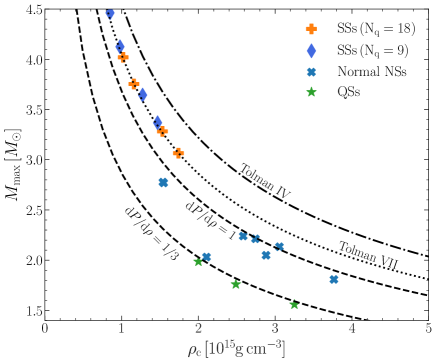
Figure 3: The relation between the maximal mass and the central mass–energy density for SSs, normal NSs, and QSs. The $M_{\rm max}$-$\rho_{\rm c}$ relation for ${\rm d}P/{\rm d}\rho=1$ and ${\rm d}P/{\rm d}\rho=1/3$ are showed. The former bounds the central densities of NSs while SSs can pass over this line. The latter effectively bounds the existence of deconfined quarks in stars. The Tolman IV and Tolman VII solutions coupled with ${\rm d}P/{\rm d}\rho=1$ are also illustrated (Lattimer & Prakash, 2005; Lattimer, 2012).

In the following sections, we will investigate the slow rotation and the tidal deformation of SSs as perturbations on the background solution of spherical and static stars that are given above.

4 Slowly rotating strangeon stars

To the order $\Omega^{3}$, the line element of a slowly rotating relativistic star is (Hartle, 1967; Hartle & Thorne, 1968; Hartle, 1973; Benhar et al., 2005)

$${\rm d}s^{2}=-e^{\nu(r)}[1+2h(r,\theta)]{\rm d}t^{2}+e^{\lambda(r)}\left[1+\frac{2m^{*}(r,\theta)}{r-2m(r)}\right]{\rm d}r^{2}$$

$$+r^{2}[1+2k_{2}(r,\theta)]\left\{{\rm d}\theta^{2}+\sin^{2}\theta[{\rm d}\phi-w(r,\theta){\rm d}t]^{2}\right\}+O(\Omega^{4})\,.$$ (14)

The metric is invariant under the combined transformations of $t\rightarrow-t$ and $\phi\rightarrow-\phi$. Therefore, the function $w(r,\theta)$ only contains odd orders of $\Omega$ while the functions $h(r,\theta)$, $m^{*}(r,\theta)$, and $k_{2}(r,\theta)$ only include the even orders of $\Omega$. We can expand these perturbative corrections with the spin-weighted spherical harmonics (Hartle, 1967, 1973).

The functions $h(r,\theta)$, $m^{*}(r,\theta)$, and $k_{2}(r,\theta)$ are of order $\Omega^{2}$ and only contain $l=0$ and $l=2$ terms,

$$h(r,\theta)= h_{0}(r)+h_{2}(r)P_{2}(\cos\theta)+O\left(\Omega^{4}\right)\,,$$ (15)

$$m^{*}(r,\theta)= m_{0}(r)+m_{2}(r)P_{2}(\cos\theta)+O\left(\Omega^{4}\right)\,,$$ (16)

$$k_{2}(r,\theta)= \left[v_{2}(r)-h_{2}(r)\right]P_{2}(\cos\theta)+O\left(\Omega^{4}\right)\,,$$ (17)

where $P_{2}(\cos\theta)$ is the Legendre polynomial with $l=2$ and the function $v_{2}(r)$ is introduced for simplicity. Note that the $l=0$ contribution to $k_{2}$ has been eliminated by a coordinate transformation. The function $w(r,\theta)$ can be expanded as (Hartle, 1973; Benhar et al., 2005)

$$w(r,\theta)=\omega(r)+w_{1}(r)-w_{3}(r)\frac{1}{\sin\theta}\frac{{\rm d}P_{3}(\cos\theta)}{{\rm d}\theta}+O\left(\Omega^{5}\right)\,.$$ (18)

Here $P_{3}(\cos\theta)$ is the Legendre polynomial with $l=3$. The function $\omega(r)$ is the $l=1$ term in the first order of $\Omega$. The functions $w_{1}(r)$ and $w_{3}(r)$ are of order $\Omega^{3}$, which represent $l=1$ and $l=3$ terms respectively.

In the Hartle-Thorne coordinate, the four-velocity of the fluid can be represented as

$$u^{t}= \left[-\left(g_{tt}+2\Omega g_{t\varphi}+\Omega^{2}g_{\varphi\varphi}\right)\right]^{-1/2}$$

$$= e^{-\nu/2}\left[1+\frac{1}{2}r^{2}\sin^{2}\theta\bar{\omega}^{2}e^{-\nu}-h_{0}-h_{2}P_{2}\right]\,,$$

$$u^{r}= u^{\theta}=0\,,\quad u^{\varphi}=\Omega u^{t}\,,$$ (19)

where the quantity,

$$\bar{\omega}(r)=\Omega-\omega(r)\,,$$ (20)

represents the angular velocity of the fluid element relative to the local inertial frame to order $\Omega$. It plays an important role in determining stellar structures.

For rotating stars, the fluid elements are displaced. To guarantee the self consistency of the perturbation theory, Hartle (1967) used a special coordinate system that maps the isodensity surface which lies at coordinate $(\tilde{R},\tilde{\Theta})$ in an unperturbed star to

$$r=\tilde{R}+\xi_{0}(\tilde{R})+\xi_{2}(\tilde{R})P_{2}(\cos\tilde{\Theta})+O(\Omega^{4})\,,\quad\theta=\tilde{\Theta}\,,$$ (21)

for the rotating star. The displacements $\xi_{0}$ and $\xi_{2}$ describe the spherical and quadrupole deformations of the star separately. In this way, the pressure and density are known functions for both of the non-rotating and rotating configurations. It is formally equivalent to work in the original ($r,\theta$) coordinate with the variations of pressure $P$, energy density $\rho$, and baryonic density $\bar{\rho}$ to be (Hartle, 1967; Hartle & Thorne, 1968)

$$\delta P= (\rho+P)\left[p_{0}+p_{2}P_{2}(\cos\theta)\right]\,,$$ (22)

$$\delta\rho= (\rho+P)\frac{{\rm d}\rho}{{\rm d}P}\left[p_{0}+p_{2}P_{2}(\cos\theta)\right]\,,$$ (23)

$$\delta\bar{\rho}= (\rho+P)\frac{{\rm d}\bar{\rho}}{{\rm d}P}\left[p_{0}+p_{2}P_{2}(\cos\theta)\right]\,.$$ (24)

The dimensionless quantities $p_{0}$ and $p_{2}$ are defined as

$$p_{0}(r)=-\xi_{0}(r)\left[\frac{1}{\rho+P}\frac{{\rm d}P}{{\rm d}r}\right]\,,\quad p_{2}(r)=-\xi_{2}(r)\left[\frac{1}{\rho+P}\frac{{\rm d}P}{{\rm d}r}\right]\,,$$ (25)

which are functions of $r$ and evaluate the pressure perturbation. Then, the stress-energy tensor of the slowly rotating star reads

$$T_{\alpha}^{\ \beta}=-(\rho+\delta\rho+P+\delta P)u_{\alpha}u^{\beta}+(P+\delta P)\delta_{\alpha}{}^{\beta}\,.$$ (26)

The structures of slowly rotating relativistic stars are determined by the perturbative functions $\omega$, $h_{0}$, $m_{0}$, $p_{0}$, $h_{2}$, $m_{2}$, $v_{2}$, $p_{2}$, $w_{1}$, and $w_{3}$, which can be calculated from systematic differential equations with appropriate boundary conditions. The types of stars that we want to solve determine the boundary conditions. A rigidly rotating star is specified by two parameters which can be diversely taken as the central density $\rho_{\rm c}$ and the angular velocity $\Omega$, or the baryonic mass $\bar{M}$ and the angular momentum $J$, or other combinations (Hartle, 1973; Stergioulas, 2003).

The constant central density sequence is commonly used and can be proceeded as follows. (I) Choose a central density $\rho_{\rm c}$ and integrate the TOV equation with a given EoS. The structure of the static and spherical background is determined. One obtains the gravitational mass $M$, the baryonic mass $\bar{M}$, and the radius of star $R$. (II) Keep the central density fixed and give a rigid angular frequency $\Omega$ to the star. Then, one calculates the corrections to the first, the second, and the third order of $\Omega$. This procedure is first formulated in Hartle (1967) to the second order of $\Omega$ and has been used in numerous literature to discuss slowly rotating relativistic stars (Hartle & Thorne, 1968; Chandrasekhar & Miller, 1974; Weber & Glendenning, 1991, 1992; Berti et al., 2005; Urbanec et al., 2013; Yagi & Yunes, 2013a, b).

An advantage of this method is that all the configurations with different angular velocities but the same central density can be obtained by rescaling a single case with a specific angular velocity. We take the angular velocity $\Omega_{*}=(M/R^{3})^{1/2}$ as the reference angular frequency in our calculations. For normal NSs, this angular frequency basically represents the limit when the matters on the equator of the star are shed. The mass $M$ and radius $R$ are that of non-rotating configuration. In practice, we first calculate a physical quantity $F^{*}_{n}$ at order $n$ for a given central density and the angular frequency $\Omega_{*}$. Then the quantity $F_{n}$ for a smaller frequency $\Omega$, where the slow rotation approximation is satisfied, can easily be obtained by

$$F_{n}=(\Omega/\Omega_{*})^{n}F^{*}_{n}\,,\quad n=1,2,3\,.$$ (27)

We present detailed differential equations and boundary conditions for $\omega$, $h_{0}$, $m_{0}$, $p_{0}$, $h_{2}$, $m_{2}$, $v_{2}$, $p_{2}$, $w_{1}$, and $w_{3}$ in the Appendix A. In the following sections, we will discuss the physical quantities related to the rotation at each order. Since the change in moment of inertia for a given baryonic mass is important in some physical processes, such as pulsar glitches and spin evolutions, we will also study the constant baryonic mass sequence in the third order of $\Omega$ and the corrections to the moment of inertia as well.

4.1 First order: Angular momentum, moment of inertia, and the dragging of the local inertial frame

The axial symmetry of the system leads to the existence of a conserved angular momentum current

$${J^{\alpha}_{\rm tot}}=T^{\alpha\beta}\eta_{\beta}\,,$$ (28)

where $\eta_{\beta}$ is the Killing vector corresponding to the rotation symmetry. A conserved total angular momentum $J_{\rm tot}$ can be defined by integrating $J_{\rm tot}^{\alpha}$ over any space-like hypersurface (Hartle & Sharp, 1967; Hartle, 1973; Misner et al., 1973). We can naturally choose the $t=\rm constant$ hypersurface and the total angular momentum is

$$J_{\rm tot}=\int J^{0}{\rm d}V=\int\sqrt{-g}T_{\ \phi}^{t}{\rm d}^{3}x=\frac{1}{8\pi}\int\sqrt{-g}R_{\ \phi}^{t}{\rm d}^{3}x\,,$$ (29)

where $g$ is the determinant of the 4-dimensional metric and ${\rm d}V=\sqrt{-g}{\rm d}^{3}x$ is the proper volume element. To the first order of $\Omega$, the star remains to be spherical and the angular momentum $J$ is of order $\Omega$,

$$J=\frac{1}{6}\left[r^{4}j(r)\frac{{\rm d}\bar{\omega}}{{\rm d}r}\right]{\bigg{|}_{r=R}}\,,$$ (30)

where we have introduced $j(r)=e^{-(\nu+\lambda)/2}$. Then the moment of inertia can be calculated with $I=J/\Omega$, which is a zeroth-order quantity and only depends on the structure of spherical and static background solution.

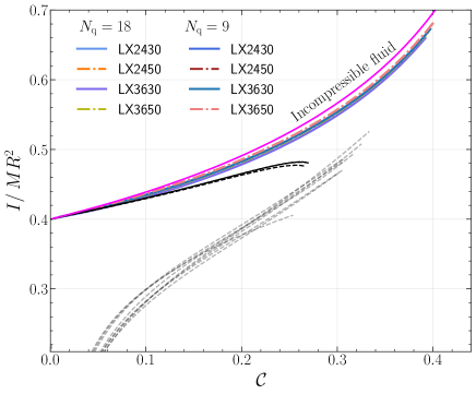
Figure 4: The relation between dimensionless moment of inertia $I/MR^{2}$ and the compactness $\mathcal{C}$ for $N_{\rm q}=18$ and $N_{\rm q}=9$. For comparison, we also plot the relations for normal NSs (grey), QSs (black), and incompressible fluid (magenta).

For normal NSs and QSs, it has been shown by Lattimer & Prakash (2001) and Bejger & Haensel (2002) that the dimensionless quantity $I/MR^{2}$ and the compactness $\mathcal{C}\equiv M/R$ satisfy two distinct EoS-insensitive quasi-universal relations. In Fig. 4, we plot the relation between $I/MR^{2}$ and $M/R$ for normal NSs and QSs. For SSs, we find that different parameters also indicate a nearly EoS-insensitive curve, which is distinct from normal NSs and also deviates from QSs in the condition of large compactness. As the compactness $M/R\rightarrow 0$, The quantity $I/MR^{2}$ for SSs and QSs tends to be the value for incompressible fluid in Newtonian gravity, namely 0.4. Moreover, as the compactness increases, QSs deviate from the incompressible fluid limit while SSs are still very close to this limit, which results from the fact that SSs have hardcore at short distances and the EoS is much stiffer than QSs.

A spinning pulsar in binary system will drag the frame and introduce relativistic spin-orbit couplings (Barker & O’Connell, 1975). This coupling between the orbit angular momentum and the spin angular momenta, also known as the Lense-Thirring precession, is related to the moment of inertia of the spinning pulsar. It produces two observable effects which could be observed with pulsar timing (Damour & Schaefer, 1988; Lattimer & Schutz, 2005). First, the spin angular momenta of the pulsars will precess around the total angular momentum of the binary system if the spin and the orbit angular momenta are not aligned. Since the total angular momentum is conserved, the precession of the spins will induce a compensating precession of the orbit angular momentum and the orbit inclination angle will change correspondingly. Second, the spin-orbit coupling makes an advance of the periastron of the orbit (Hu et al., 2020).

The spin of one star (component $\rm A$) usually spins much faster than the companion (component $\rm B$). The contribution to the Lense-Thirring effect of star $\rm B$ can usually be neglected. The precession of the orbital plane causes a periodic deviation of the time-of-arrival of pulses from pulsar $\rm A$. The period departure is proportional to $I_{\rm A}\Omega_{A}\cos i$ (Lattimer & Schutz, 2005), where $I_{\rm A}$ and $\Omega_{\rm A}$ are the moment of inertia and spin angular velocity of pulsar A, and $i$ is the inclination angle of the orbit plane. The periastron advance due to Lense-Thirring effect is proportional to $I_{\rm A}\Omega_{A}$, which is a tiny effect compared to the first post-Newtonian (PN) term and is opposite to the direction of orbital motion. One can notice that the moment of inertia will enter into those observational effects. Thus the search of Lense-Thirring effect of pulsars will tell us information on the moment of inertia.

The most promising candidate of detecting Lense-Thirring precession is the double pulsar system PSR J0737$-$3039A/B. This relativistic system (orbital period $\simeq 2.45\,\rm h$) contains two pulsars with spin period $P_{\rm A}\simeq 22\,\rm ms$ and $P_{\rm B}$ about 122 times larger than A (Burgay et al., 2003). One can neglect the contribution to Lense-Thirring effect of pulsar B. The angle between the spin angular momentum of pulsar A and the orbital angular momentum is very small, which makes the periodic modulations due to the precession of the orbital plane hard to measure since $\cos i\simeq 0$. However, it is found that the advance of the periastron is possible to be measured to a accuracy of $\sim 10\%$ in several years of timing (Kramer & Wex, 2009). This measurement can put important constraints on the EoS of NSs (Lattimer & Schutz, 2005). Recently, Hu et al. (2020) investigated the prospects for constraining the moment of inertia of pulsar A in details by simulating the timing observations with the MeerKAT and the SKA (Shao et al., 2015; Weltman et al., 2020). The results suggest a measurement of moment of inertia $I_{\rm A}$ to an accuracy of $11\%$ at 68$\%$ confidence level.

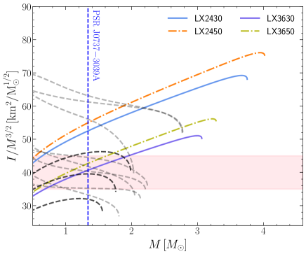
Figure 5: The relation between the rescaled moment of inertia $I/M^{3/2}$ and mass of stars $M$. The relations for normal NSs (grey dashed lines) and QSs (black dashed lines) are also displayed. The vertical line represents the mass of PSR 0737$-$3039A, $M=1.338M_{\odot}$. The pink shaded region denotes a hypothetical $10\%$ measurement of the moment of inertia for PSR 0737$-$3039A with its center value $40\,{\rm km^{2}}/M^{1/2}_{\odot}$.

In Fig. 5, we plot the relations between the rescaled moment of inertia $I/M^{3/2}$ (to reduce the range of the coordinate) and mass of stars $M$ for SSs with $N_{\rm q}=18$, normal NSs, and QSs. For normal NSs, the rescaled moment of inertia is nearly monotonically decreasing with respect to the increase of mass. While the relations for QSs and SSs are inverse except for very large masses. We also plot a hypothetical $10\%$ measurement of the quantity $I/M^{3/2}$ for PSR 0737$-$3039A (Hu et al., 2020) with the central value to be $40\,{\rm km^{2}}/M^{1/2}_{\odot}$. If this is the case, some stiff EoSs of normal NSs, as well as EoSs LX2430 and LX2450 of SSs with $N_{\rm q}=18$, will be excluded.

For given $N_{\rm q}$, the EoS of SSs in the Lennard Jones model is determined by two parameters, the potential depth $\epsilon$ and the surface baryonic number density $n_{\rm s}$. Each pair of $\epsilon$ and $n_{\rm s}$ also corresponds to a specific maximal mass of SSs and a unique moment of inertia for PSR 0737$-$3039A. Therefore, in Fig. 6 and Fig. 7, we plot the contour lines for maximal mass and moment of inertia spanning across the parameter space of $\epsilon$ and $n_{\rm s}$ for $N_{\rm q}=18$ and $N_{\rm q}=9$ respectively. If the moment of inertia of PSR 0737$-$3039A is measured in the future, one can put constraints on the parameter space of $\epsilon$ and $n_{\rm s}$, and the maximal mass of SSs.

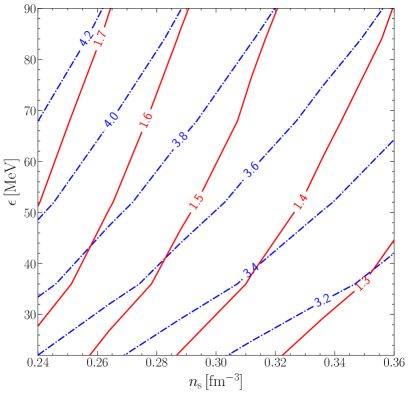
Figure 6: Contours of maximal masses $M_{\rm max}$ (blue) and moment of inertia $I_{45}$ ($I/10^{45}\,\rm g\,cm^{2}$) of PSR 0737$-$3039A (red) for SSs with $N_{\rm q}=18$.

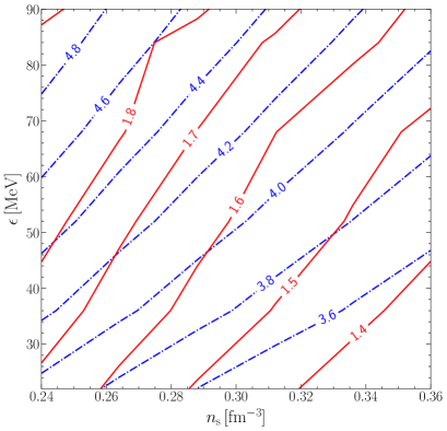
Figure 7: Same as Fig. 6, for $N_{\rm q}=9$.

4.2 Second order: Spherical and quadrupole deformations

As we mentioned before, to the second order of $\Omega$, the star will be deformed and the isodensity surface at radial coordinate $r$ in the non-rotating star will be displaced to $r+\xi_{0}(r)+\xi_{2}(r)P_{2}(\cos\theta)$ in the rotating configuration (Hartle & Thorne, 1968). According to the definition of the “pressure perturbation factor” $p_{0}$ and $p_{2}$ in Eq. (25), the displacements $\xi_{0}$ and $\xi_{2}$ can be represented as,

$$\xi_{0}(r)= -p_{0}(\rho+P)/({\rm d}P/{\rm d}r)=p_{0}\,r(r-2m)/(m+4\pi r^{3}P)\,,$$ (31)

$$\xi_{2}(r)= -p_{2}(\rho+P)/({\rm d}P/{\rm d}r)=p_{2}\,r(r-2m)/(m+4\pi r^{3}P)\,,$$ (32)

which are second order of $\Omega$ and are related to the spherical and quadrupole deformations respectively. Correspondingly, the perturbative functions of order $\Omega^{2}$ can be divided into two classes: (i) the $l=0$ functions, $m_{0}$, $h_{0}$, and $p_{0}$, that describe the spherical stretching of the star; (ii) the $l=2$ functions, $h_{2}$, $v_{2}$, $m_{2}$, and $p_{2}$, that describe the quadrupole deformation of the star.

One may directly use $\xi_{0}(r)$ and $\xi_{2}(r)$ to define the mean radius and the eccentricity of the isodensity surface in the Hartle-Thorne coordinate (Hartle, 1967; Hartle & Thorne, 1968),

$$\bar{r}_{\rm HT}= \,r+\xi_{0}(r)\,,$$ (33)

$$e(r)_{\rm HT}= \left[\text{ (radius at equator) }^{2}/(\text{ radius at pole })^{2}-1\right]^{1/2}$$

$$= \left[-3\xi_{2}(r)/r\right]^{1/2}\,,$$ (34)

which are not invariant under the transformation of coordinate system. To give an invariant parametrization of the isodensity surface, one needs to embed the geometry into a three-dimensional flat space (denoted with polar coordinates $r^{*}$, $\theta^{*}$, and $\phi^{*}$) and search for the surface that has the same intrinsic geometry as the isodensity surface of the star (Hartle & Thorne, 1968; Chandrasekhar & Miller, 1974).

To the second order of $\Omega$, the desired surface in flat space is a spheroid with the equation (Hartle & Thorne, 1968)

$$r^{*}\left(\theta^{*}\right)=r+\xi_{0}(r)+\Big{\{}\xi_{2}(r)+r\left[v_{2}(r)-h_{2}(r)\right]\Big{\}}P_{2}\left(\cos\theta^{*}\right)\,.$$ (35)

The mean radius of the spheroid is

$$\bar{r}^{*}=r+\xi_{0}(r)\,,$$ (36)

and the eccentricity can be defined as

$$e(r) =\left[\text{ (radius at equator) }^{2}/(\text{ radius at pole })^{2}-1\right]^{1/2}$$

$$=\left[-3\left(v_{2}-h_{2}+\xi_{2}/r\right)\right]^{1/2}\,.$$ (37)

The mean radius of the star, $\bar{R}$, and the eccentricity of the surface of the star, $e_{\rm s}$, can be obtained by setting $r=R$.

Since the fluid elements are displaced and the star comes to a new equilibrium state, the baryonic mass, the gravitational mass, and the quadrupole moment also change. To obtain the deformation of the star and changes in various physical quantities, we need to give the solutions of the $l=0$ and $l=2$ perturbative functions. Numerically, One integrates the differential equations of those perturbative functions in Appendix A with appropriate boundary conditions at the center of the star and at infinity. Fortunately, the analytical solutions exist outside of the star with some undetermined constants. One therefore can integrate the differential equations for perturbative functions to the radius $R$ and match the results with the exterior solutions to ascertain the undetermined constants.

A technical problem needs to be stressed. For SSs or QSs, the surface density drops from nuclear densities to zero and some thermodynamical quantities such as pressure do not admit regular Taylor expansions in $(r-R)$ when $r\rightarrow R$ (Damour & Nagar, 2009). For example, the differential equations involving the terms $(\rho+P)\mathrm{d}\bar{\rho}/\mathrm{d}P$ or $(\rho+P)\mathrm{d}\rho/\mathrm{d}P$ are singular across the surface of the star. To solve the issue, one can treat the baryonic density $\bar{\rho}(r)$ and the mass-energy density ${\rho}(r)$ as inverted step functions across the surface of the star. Then the terms $(\rho+P)\mathrm{d}\bar{\rho}/\mathrm{d}P$ and $(\rho+P)\mathrm{d}\rho/\mathrm{d}P$ at the boundary of the star can be represented as

$$\frac{\mathrm{d}\bar{\rho}}{\mathrm{d}P}(\rho+P)= \bar{\rho}\delta(r-R)r(r-2m)/(m+4\pi r^{3}P)\,,$$ (38)

$$\frac{\mathrm{d}{\rho}}{\mathrm{d}P}(\rho+P)= {\rho}\delta(r-R)r(r-2m)/(m+4\pi r^{3}P)\,,$$ (39)

where we have used the expression of ${\rm d}P/{\rm d}r$ in Eq. (12). Numerically, we first integrate the differential equations in the open interval $0<r<R$ and obtain the value $y(R_{-})$ just inside of the star, where $y$ is a physical quantity depending on the radial coordinate $r$. Second, we add the contributions from the integration of $\delta$ function at the surface of the star and get the value just outside of the star $y(R_{+})$. Then, the undetermined constants are obtained by matching $y(R_{+})$ with the exterior solutions. Physically, it means that one must consider the match conditions to guarantee the continuity of spacetime. The physical quantities in the interior of the star $\Sigma^{-}$ and the exterior vacuum region $\Sigma^{+}$ are matched on a common boundary $\Sigma_{0}=\Sigma^{\pm}(r=R_{\pm})$. For convenience, we define $[y]:=y^{+}\big{|}_{\Sigma_{0}}-y^{-}\big{|}_{\Sigma_{0}}$ (Reina, 2016; Reina et al., 2017).

4.2.1 Spherical deformations: change in the gravitational mass and the baryonic mass

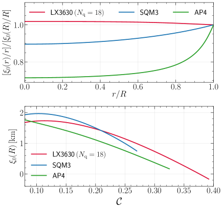
Figure 8: The spherical stretching due to rotation. For clarity, we only shows the results for EoS LX3630 ($N_{\rm q}=18$), AP4, and SQM3. The upper panel shows the fractional change $\xi_{0}(r)/r$ of the isodensity surface at the radial coordinate $r$, normalized by the fractional change $\xi_{0}(R)/R$ at the surface of the star, where we take $M=1.4\,M_{\odot}$ for the non-rotating configuration. In the lower panel, we display the relation between the spherical displacement at the surface of the star $\xi_{0}(R)$ and the compactness $\mathcal{C}$. We take the angular frequency to be $\Omega_{*}$. For a fixed central density, the stretching at the surface $\xi_{0}(R)$ for a smaller angular velocity $\Omega$ can be obtained by multiplying the factor $(\Omega/\Omega_{*})^{2}$.

In the upper panel of Fig. 8, we show the fractional change $\xi_{0}(r)/r$ of the isodensity surface at the radial coordinate $r$ normalized by the fractional change $\xi_{0}(R)/R$ at the surface of the star. The behaviors of $(\xi_{0}(r)/r)/(\xi_{0}(R)/R)$ reveal the density distribution inside of the star (Hartle & Thorne, 1968). For an EoS of normal NSs, AP4, the star has a dense core and an envelope, and the density distribution is more diffusive than the EoS of SSs and QSs. As a consequence, the spherical stretching is small in the core and increases in the envelope of the star. For SSs and QSs, the densities inside of the star are more homogeneous than normal NSs, and the variations of the fractional stretching are smaller. This tendency is just what we expect from simple Newtonian intuition. Particularly, the fractional change of the stretching of the SSs is nearly a constant through the star, which indicates that the EoS of SSs is close to the incompressible fluid. Besides, for SSs, the fractional change $\xi_{0}(r)/r$ decreases monotonically from the center to the boundary of the star, which is different from QSs and normal NSs.

In the lower panel of Fig. 8, we plot the spherical stretching $\xi_{0}(R)$ versus the compactness of the star. The spherical stretching decreases with the increase of the compactness in the case of $M/R\geq 0.1$. Another feature is that the spherical stretching can be smaller than zero near the maximal mass for SSs. The “pressure perturbation factor” $p_{0}$ is negative and the rotation makes the star contract. Chandrasekhar & Miller (1974) also showed this feature for incompressible fluid when $R/R_{\rm s}\rightarrow 9/8$, where $R_{\rm s}$ is the Schwarzschild radius (see the first three columns of Table I and Figure 3 therein).

The baryonic mass and the gravitational mass are rotational invariant quantities and do not change under parity transformation ($\Omega\rightarrow-\Omega$). Thus, perturbations are only determined by the $l=0$ functions, namely $h_{0}$, $m_{0}$, and $p_{0}$, and the non-rotating background solutions. In practice, we numerically integrate $m_{0}$ and $p_{0}$ inside of the star. Outside of the star, $p_{0}$ vanishes and $m_{0}$ is

$$m_{0}=\ \delta M-J^{2}/r^{3}\,,$$ (40)

where $\delta M$ is a constant and $J$ is the angular momentum. The interior and the exterior solutions are matched at $r=R$ with the match condition

$$[m_{0}]=4\pi R^{3}\rho\left(R_{-}\right)(R-2M)p_{0}(R)/M\,,$$ (41)

where $\rho\left(R_{-}\right)$ represents the energy density just inside of the star. The function $h_{0}$ can be obtained by algebraic relations

$$h_{0}= -p_{0}+\frac{1}{3}r^{2}e^{-\nu}\bar{\omega}^{2}+h_{0\rm c}\,,\quad(\rm inside\ of\ the\ star),$$ (42)

$$h_{0}= -\frac{\delta M}{r-2M}+\frac{J^{2}}{r^{3}(r-2M)}\,,\quad(\rm outside\ of\ the\ star).$$ (43)

The constant $h_{0\rm c}$ is the value of $h_{0}$ at the center of the star, which can be obtained by matching the interior and exterior solutions.

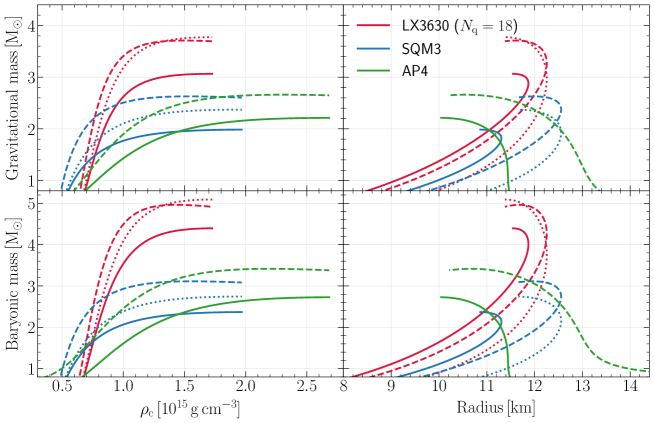
Figure 9: The first column shows the the gravitational mass and the baryonic mass versus the central mass-energy density for representative EoSs $\rm LX3630\,(N_{\rm q}=18)$, SQM3, and AP4. The solid lines represent non-rotating configurations. The dashed lines are the ones for rotating configurations with the angular frequency $\Omega_{*}$. The gravitational mass and the baryonic mass for a smaller frequency $\Omega$, where the slow rotation approximation is valid, can be easily obtained by an upward displacement from the solid curves by the fraction $(\Omega/\Omega_{*})^{2}$ of the distance to the dashed curves (see text for more details). The second column shows the relation between the gravitational mass and the mean radius. The solid curves are plots of the mass $M$ versus the radius $R$ for non-rotating stars. The dashed curves represent the relation between mass $\mathcal{M}=M+\delta M$ and mean radius $\bar{R}=R+\xi_{0}(R)$ for rotating configurations with angular frequency $\Omega_{*}$. The mass radius relations for angular velocities that satisfies the slow rotation approximation can be obtained by multiplying the rescaling factor $(\Omega/\Omega_{*})^{2}$ along a constant central density sequence. For comparison, we also display the relations for $\rm LX3630\,(N_{\rm q}=18)$, SQM3 without the corrections induced by the match conditions with dotted lines.

In general relativity, the mass $\mathcal{M}$ of a rotating relativistic star is determined by the spherical part of the metric $g_{tt}$ at large distances

$$-\frac{1+g_{tt}}{2}\Big{|}_{\rm spherical\ part}=-\frac{\mathcal{M}}{r}\,,\quad r\rightarrow\infty\,.$$ (44)

Combining the metric of a slowly rotating relativistic star in Eq. (4) and the exterior solution of $h_{0}$ in Eq. (43), one obtains the total gravitational mass

$$\mathcal{M}=M+\delta M\,,$$ (45)

where $M$ is the background contribution and $\delta M$ is the second order correction which appears as an integration constant in the exterior solution of $h_{0}$ and $m_{0}$. After matching the interior and the exterior solutions of $m_{0}$, one obtains

$$\delta M=m_{0}(R_{-})+4\pi R^{3}\rho(R_{-})(R-2M)p_{0}(R)/M+J^{2}/R^{3}\,.$$ (46)

The baryonic mass is a conserved quantity. Integrating the differential form of the baryonic mass conservation law, $\big{[}\sqrt{-g}\bar{\rho}u^{\mu}\big{]}_{,\mu}=0$, at a $t=\rm const$ hypersurface, one obtains the baryonic mass of the star (Hartle, 1967; Misner et al., 1973)

$$\bar{\mathcal{M}}=\int\sqrt{-g}\bar{\rho}u^{t}{\rm d}^{3}x\,.$$ (47)

Note that the integration extends to the whole region of the deformed star. To second order of $\Omega$, the expansion of the baryonic mass can be represented as $\bar{\mathcal{M}}=\bar{M}+\delta\bar{M}+O(\Omega^{4})$. The baryonic mass of the non-rotating star is

$$\bar{M}=\int^{R}_{0}4\pi r^{2}\left(1-\frac{2m}{r}\right)^{-1/2}\bar{\rho}{\rm d}r\,.$$ (48)

The correction at the second order of $\Omega$ is

$$\delta\bar{M} =\int_{0}^{R}4\pi r^{2}\left(1-\frac{2m}{r}\right)^{-1/2}$$

$$\times\bigg{\{}\Big{[}\frac{m_{0}}{r-2m}+\frac{1}{3}r^{2}\bar{\omega}^{2}e^{-\nu(r)}\Big{]}\bar{\rho}+\frac{{\rm d}\bar{\rho}}{{\rm d}P}(\rho+P)p_{0}\bigg{\}}{\rm d}r\,,$$ (49)

which can be represented as

$$\delta\bar{M}=\delta\bar{M}(R_{-})+4\pi R^{3}\left(1-\frac{2M}{R}\right)^{-1/2}\frac{\bar{\rho}(R_{-})(R-2M)p_{0}(R)}{M}\,,$$ (50)

where we have considered the corrections from the matching condition at the surface of the star.

In Fig. 9, we show the gravitational mass and the baryonic mass at frequency $\Omega_{*}$ for EoS LX2430 ($N_{\rm q}=18$), SQM3, and AP4. The slow-rotation approximation breaks down at this frequency. But the mass and the radius for a given central density and a smaller angular frequency $\Omega$ can be simply obtained by multiplying the factor $(\Omega/\Omega_{*})^{2}$. The maximal mass at the rotating frequency $\Omega_{*}$ increases by $\sim 20\%$. We also plot the lines without the corrections from the match conditions at the surface of the star. It is obvious that the corrections are crucial and cannot be ignored.

4.2.2 Quadrupole deformations: the production of quadrupole moments

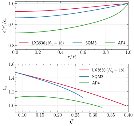
Figure 10: The upper panel shows the eccentricity $e(r)$ of isodensity surface at radial coordinate $r$, normalized by the eccentricity $e_{\rm s}$ at the surface of the star, where the mass for the non-rotating configuration is taken as $M=1.4\,M_{\odot}$. The lower panel shows the relation between the surface eccentricity $e_{\rm s}$ and the compactness $\mathcal{C}$ with the angular frequency chosen to be $\Omega_{*}$. For a smaller frequency $\Omega$ where the slow-rotation approximation is valid, the surface eccentricity $e_{\rm s}$ can be obtained by multiplying the factor $\Omega/\Omega_{*}$ for a fixed central density.

The quadrupole deformation can be described by the eccentricity $e(r)$ of the isodensity surface at radial coordinate $r$. In the upper panel of Fig. 10, we show the fractional change of the eccentricity $e(r)/e_{\rm s}$ at different radial coordinates inside of the star. The relations also reveal the internal density distribution, which has the same tendencies as the fractional change of the radial stretching in the upper panel of Fig. 8. The relation between the surface eccentricity $e_{\rm s}$ and the compactness $\mathcal{C}$ is shown in the lower panel of Fig. 10, where we set the angular frequency to be $\Omega_{*}$. One can notice that the surface eccentricity for LX2430 and SQM3 are larger than that of AP4. The difference between SSs and normal NSs can be as large as $\sim 20\%$ for some choices of the compactness.

The quadrupole moment depends on the $l=2$ perturbative functions: $h_{2}$, $v_{2}$, $p_{2}$, and $m_{2}$. In practice, we integrate the differential equations to obtain the interior solutions of $h_{2}$ and $v_{2}$. The exterior solutions of $h_{2}$ and $v_{2}$ are

$$h_{2}= J^{2}\left(\frac{1}{Mr^{3}}+\frac{1}{r^{4}}\right)+KQ_{2}^{2}\left(\frac{r}{M}-1\right)\,,$$ (51)

$$v_{2}= -\frac{J^{2}}{r^{4}}+K\frac{2M}{[r(r-2M)]^{1/2}}Q_{2}^{1}\left(\frac{r}{M}-1\right)\,,$$ (52)

where $Q_{2}^{1}$ and $Q_{2}^{2}$ are the associated Legendre functions of the second kind. The constant $K$ is determined by matching the exterior and interior solutions at $r=R$ with the match conditions

$$[h_{2}]=0\,,\quad[v_{2}]=0\,.$$ (53)

The functions $p_{2}$ and $m_{2}$ can be obtained from the algebraic relations (Hartle & Thorne, 1968),

$$m_{2}= \ (r-2m)\left[-h_{2}-\frac{1}{3}r^{3}\left({\rm d}j^{2}/{\rm d}r\right)\bar{\omega}^{2}+\frac{1}{6}r^{4}j^{2}({\rm d}\bar{\omega}/{\rm d}r)^{2}\right]\,,$$ (54)

$$p_{2}= -h_{2}-\frac{1}{3}r^{2}e^{-\nu}\bar{\omega}^{2}\,,$$ (55)

which come from the first integrals of the Einstein field equations.

The quadrupole moment can be read out from the coefficient of $P_{2}(\cos\theta)/r^{3}$ in the Newtonian potential (Hartle & Thorne, 1968; Thorne & Hartle, 1984). As the radial coordinate $r$ goes to infinite asymptotically, the quadrupole part of the Newtonian potential is

$$-\frac{1+g_{tt}}{2}\Big{|}_{\rm quadrupole\ part}=-\frac{Q_{\rm r}}{r^{3}}P_{2}(\cos\theta)\,,\quad r\rightarrow\infty\,,$$ (56)

where $Q_{\rm r}$ is the rotation-induced quadrupole moment. Calculating the effective potential $-(1+g_{tt})/2$ with the expansion of $h_{2}$ in Eq. (51) at large distance and comparing the results with the formal expression in Eq. (56), one obtains the quadrupole moment of the star

$$Q_{\rm r}=-\frac{J^{2}}{M}-\frac{8}{5}KM^{3}\,.$$ (57)

Here, $Q_{\rm r}<0$ means that the star is deformed into an oblate shape. Note that the quadrupole moments not only depend on the spin angular momentum of the star, but also depend on the integration constant $K$, which is related to the EoS. For black holes, the quadrupole moment is $Q_{\rm r}=-J^{2}/M$, which only depends on the angular momentum and the mass of the black hole. This property is guaranteed by the no hair theorem. One usually define the dimensionless quadrupole moment,

$$\bar{Q}\equiv-\frac{Q_{\rm{r}}}{M^{3}\chi^{2}}\,.$$ (58)

Similarly, the dimensionless spin $\chi$ is defined as $\chi\equiv J/M^{2}$.

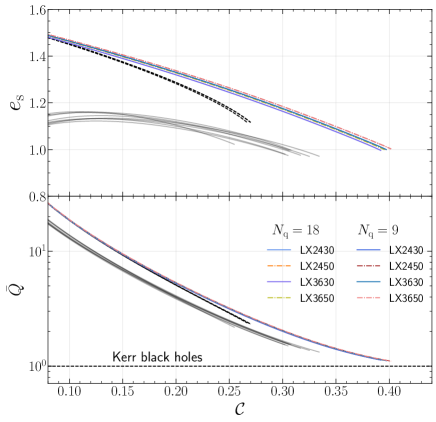
Figure 11: The upper panel shows the relation between the surface eccentricity and the compactness for SSs with $N_{\rm q}=18$ and $N_{\rm q}=9$, normal NSs (grey), and QSs (black). This panel is the same as the lower panel of Fig. 10 but more EoSs are included. The lower panel displays the relation between the dimensionless quadrupole moment and the compactness for SSs with $N_{\rm q}=18$ and $N_{\rm q}=9$, normal NSs (grey), and QSs (black). The horizontal line represents the dimensionless quadrupole moment of Kerr black holes, where $\bar{Q}=1$.

In Fig. 11, we plot the surface eccentricity $e_{\rm s}$ and the dimensionless quadrupole moment $\bar{Q}$ for SSs, QSs, and normal NSs. There is a quasi-universal relation between $e_{\rm s}$ and $\mathcal{C}$. While the universality of the relation between the dimensionless quadrupole moment $\bar{Q}$ and $\mathcal{C}$ is tighter. For NSs, the universal relation is quite different from the ones for QSs and SSs. The $\bar{Q}$–$\mathcal{C}$ universal relation for normal NSs and QSs has been discovered by Urbanec et al. (2013). For SSs, the universal relation is nearly undistinguishable from that of QSs at small compactness. But as the compactness increases, the quadrupole of SSs becomes larger than that of QSs. This feature also appears in the universal relations of moment of inertia shown in Fig. 4. The reason is again that SSs are much stiffer than QSs at high densities.

The quadrupole moment $\bar{Q}$ and the surface eccentricity $e_{\rm s}$ both describe the departure from spherical symmetry of the stars. Therefore, $\bar{Q}$ and $e_{\rm s}$ show common features: (i) for a given compactness, the quadrupole moment and the surface eccentricity of SSs are larger than QSs, while the quantities of QSs are larger than that of the normal NSs; (ii) the quadrupole moment and the surface eccentricity both decrease as the compactness increases in the range we plot. The quadrupole moment tends to be close to the limit of Kerr black holes. For our models of SSs, this tendency is very clear and $\bar{Q}$ is very close to 1 for the stars near the maximal compactness (corresponding to the maximal mass). So, it is hard to distinguish Kerr black holes and rotating SSs around maximal mass purely from these two quantities.

We also show the relations between the quadrupole moments and the masses of the stars in Fig. 12. A key feature is that the quadrupole moments decrease with the increase of the masses for all of EoS that we consider. The quadrupole moments also depend on the EoS strongly to some extent. For example, the dimensionless quadrupole moment $\bar{Q}$ can range from $\sim 2$ to $\sim 8$ at $1.4\,M_{\odot}$ for the EoSs we selected. Thus, The measurements of the quadrupole moments can give constraints on the EoS. In Fig. 13 and Fig. 14, we display the contours of maximal mass and quadrupole moment at $1.4\,M_{\odot}$ for SSs with $N_{\rm q}=18$ and $N_{\rm q}=9$. The constraints on quadrupole moments can be used to constrain the parameter space of $\epsilon$ and $\sigma$.

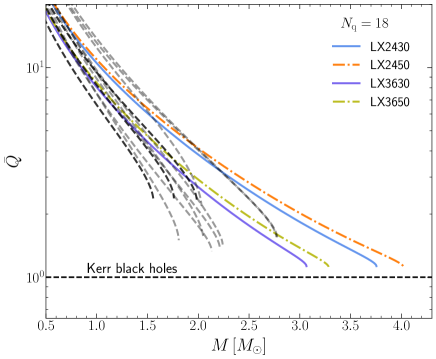
Figure 12: The dimensionless quadrupole moment versus the mass $M$ of non-rotating stars for SSs with $N_{\rm q}=18$. The relations for $N_{\rm q}=9$ have the similar trend and we ignore them for clarity of the figure. For comparison, the relations for normal NSs (grey) and QSs (black) are also plotted. The horizontal line represents the dimensionless quadrupole moment of Kerr black holes, where $\bar{Q}=1$.

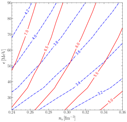
Figure 13: Contours of maximal masses $M_{\rm max}$ (blue) and dimensionless quadrupole moments with $M=1.4\,M_{\odot}$ (red) for $N_{\rm q}=18$.

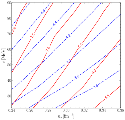
Figure 14: Same as Fig. 13, but for $N_{\rm q}=9$.

The pulsed emission of X-rays originating from the surface of rotating NSs contains the information of the strong-filed regime around the NSs, which can be characterized by the global properties which mainly consist of mass, radius, and spin frequency. Detailed modelling of the emission region on the stellar surface combined with the relativistic null geodesic of photons can be used to construct theoretical light curves, which can then be compared with the observed light curves to probe the masses and radii, and then constrain the EoS of the NSs (Morsink et al., 2007; Watts et al., 2016).

Some of the targets for X-ray observations have moderate spins $\sim 300$–$700\,\rm Hz$ (Bogdanov et al., 2008). Besides the masses and radii, the quadrupole moments and the eccentricity of the stars also affect the light curves of X-rays (Morsink et al., 2007; Bauböck et al., 2013b). Morsink et al. (2007) considered the quadrupole moment and the shape of the NSs when modelling the X-ray profiles. It is the so-called oblate-Schwarzschild approximation (OS). It is found that the quadrupole moment and the eccentricity are important in modelling the light curves, and for some emission geometries, the deformations of the stars can rival the Doppler effects (Morsink et al., 2007). The main reason is that the oblate shape will make some certain spot locations visible that would be invisible in the spherical cases, and vice versa. Bauböck et al. (2013a); Bauböck et al. (2013b) showed that the quadrupole moments can also induce features with narrow peaks in the X-ray flux and they also found that the shape parameters calculated with Hartle-Thorne approximation are consistent with the numerical results obtained by Morsink et al. (2007) to an accuracy of $1\%$ for observed spin frequencies.

On one hand, the universal relations between different quantities (such as $\bar{Q}$ and $\mathcal{C}$, $e_{\rm s}$ and $\mathcal{C}$) can help to decrease the dimensions of parameter space when modelling the profiles (Bauböck et al., 2013b). On the other hand, the difference of the universality for normal NSs, QSs, and SSs might be used to determine whether the pulsars are gravitationally bound or self-bound.

Now the NICER satellite is taking data from some X-ray pulsars and has given certain constraints on the radii of NSs (Miller et al., 2019; Riley et al., 2019) and the OS approximation is commonly used in the modelling of X-ray profiles. In the future, the observations may also give constraints on the quadrupole moments and the shapes of rotating stars.

For binary systems involving NSs, the quadrupole moments also contribute to GW radiations through the quadrupole-monopole interactions (Poisson, 1998; Yagi & Yunes, 2013a; Isoyama et al., 2018; Harry & Hinderer, 2018). The leading order effect enters into the waveform at the 2 PN order, and the correction to the GW phase is roughly proportional to $\sim\bar{Q}\chi^{2}$ (Poisson, 1998; Harry & Hinderer, 2018). Physically, it is a Newtonian effect despite the scaling has the form of PN expansion. It may be possible to measure or constrain the quadrupole moment with GWs. Yagi & Yunes (2013a) performed GW data analysis for binary NSs and evaluated the possibility to constrain quadrupole moments with the next generation ground-based GW detector ET, and space-based detectors DECIGO/BBO. They found that although the quadrupole moments are hard to measure due to the strong correlations with the spins of NSs, at least one can put upper bounds on the quadrupole moments. If the NSs in the binary systems rotate rapidly, then the measurement of quadrupole moments is possible (Isoyama et al., 2018; Yagi & Yunes, 2013a; Liu & Shao, 2021).

4.3 Third order: Corrections to the angular momentum and the moment of inertia

Taking the integral in Eq. (29) and extending over the region that is interior to the isodensity surface given by $R+\xi_{0}(R)+\xi_{2}(R)P_{2}(\theta)$, one finds that only odd orders of $\Omega$ contribute to the angular momentum. At the third order of $\Omega$,

$$\delta J=-\frac{1}{6}\left\{r^{4}j\frac{\mathrm{d}w_{1}}{\mathrm{~{}d}r}+r^{4}j\frac{\mathrm{d}\bar{\omega}}{\mathrm{d}r}\left[h_{0}+\frac{m_{0}}{r-2m}+\right.\right.$$

$$\left.\left.+\frac{1}{5}\left(4v_{2}-5h_{2}-\frac{m_{2}}{r-2m}\right)\right]+4r^{3}\frac{\mathrm{d}j}{\mathrm{~{}d}r}\bar{\omega}\left(\xi_{0}-\frac{1}{5}\xi_{2}\right)\right\}{\bigg{|}_{r=R_{+}}}\,.$$ (59)

The moment of inertia at the second order of $\Omega$ is $\delta I=\delta J/\Omega$. Note that each term in the above expression is evaluated at $r=R_{+}$ and the match conditions for $m_{0}$, $m_{2}$, and $r^{4}j{\rm d}w_{1}/{\rm d}r$ at the boundary need to be considered for SSs and QSs. The details can be found in the Appendix A.

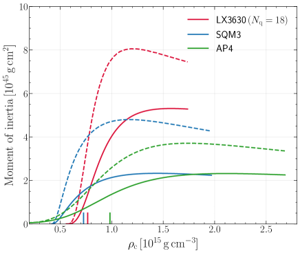
Figure 15: The moment of inertia versus central mass-energy density. The solid lines are the moment of inertia for non-rotating configuration. The dashed lines are moment of inertia with the rotation angular frequency $\Omega_{*}$. The moment of inertia for a smaller frequency $\Omega$, where the slow rotation approximation is valid, can be easily obtained by an upward displacement from the solid curves by the fraction $(\Omega/\Omega)^{2}$ of the distance to the dashed curves. We choose EoS LX3630 ($\,N_{\rm q}=18$), SQM3, and AP4 in the plot. The short vertical lines at the bottom of the figure represent the central mass-energy density of non-rotating configuration with $M=1.4M_{\odot}$.

In Fig. 15, we plot the $\delta I+I$ and $I$ for representative EoSs for SSs, QSs, and normal NSs. Note that we take the angular frequency to be $\Omega_{*}$. The moment of inertia for a lower frequency $\Omega$ at a specific central density can be easily obtained by multiplying the rescaling factor $(\Omega/\Omega_{*})^{2}$.

Under some conditions, we are interested in computing the moment of inertia as a function of the angular velocity for a star with given baryonic mass (e.g., the glitch processes and the spin evolution of newly-born NSs). Hartle (1973) first constructed the constant baryonic sequence based on his early work (Hartle, 1967), and the procedures are as follows:

1. Same as the first step in the constant density sequence, one obtains baryonic mass $\bar{M}$, gravitational mass $M$, and the radius of the star $R$ from the static and non-spinning configuration.

2. The structures are calculated to the second order with the same central density. In order to obtain the same baryonic mass $\bar{M}$, one imposes that the boundary value of $p_{0}$ and $m_{0}$ deviate from zero at the center of the star until the corrections to baryonic mass $\delta\bar{M}$ is equal to zero. This means that the central density is perturbed from background value $\rho_{\rm c}$.

3. Calculate the third order perturbations based on the boundary conditions used in the second step.

The central idea of Hartle’s approach is treating the change of central density $\delta{\rho_{\rm c}}$ as a perturbation. This assumption will breakdown in two cases. First, when the star rotates sufficiently rapid, $\delta{\rho_{\rm c}}$ is actually not a small value and this procedure will produce large errors to other quantities (Benhar et al., 2005). The second breakdown appears when the mass of the star is close to the maximal mass (Hartle, 1973). We denote the rotational perturbation of the baryonic mass in the constant density sequence as $\delta\bar{M}(\rho_{\rm c},\Omega)$. Now we want to construct a rotating star with the same baryonic mass by perturbing the central density. The variation of the baryonic mass is

$$\delta\bar{M}(\rho_{\rm c},\Omega)=\left.\frac{\partial\bar{M}}{\partial\Omega}\right|_{\rho_{\rm c}}\delta\Omega+\left.\frac{\partial\bar{M}}{\partial\rho_{\rm c}}\right|_{\Omega}\delta\rho_{\rm c}=0\,.$$ (60)

It follows that for a given baryonic mass (Hartle, 1973; Benhar et al., 2005)

$$\left.\frac{\partial\rho_{\rm c}}{\partial\Omega}\right|_{\bar{M}}=-\bigg{(}\left.\frac{\partial\bar{M}}{\partial\Omega}\right|_{\rho_{\rm c}}\bigg{)}\bigg{/}\bigg{(}\left.\frac{\partial\bar{M}}{\partial\rho_{\rm c}}\right|_{\Omega}\bigg{)}\,.$$ (61)

When the sequence is close to the maximal mass, the term $\partial\bar{M}/\partial\rho_{\rm c}|_{\Omega}\rightarrow 0$. Consequently, the change of the central density $\partial\rho_{\rm c}/\partial\Omega|_{\bar{M}}\rightarrow\infty\,$, which violates the assumption that the change of central density is a small correction and this approach fails. The solutions become unstable near the maximal masses as shown in Hartle (1973).

Benhar et al. (2005) formulated another procedure to obtain the constant baryonic mass sequence based on Hartle (1973). The procedure is as follows:

1. Same as the first step in the Hartle’s constant density sequence, one can obtain a baryonic mass $\bar{M}$ for an assigned EoS and central density $\rho_{\rm c}$.

2. Choosing an angular velocity $\Omega$ and integrating the perturbed equations to the third order of $\Omega$ for various values of $\rho_{\rm c}$, one can get a branch of solutions with the same angular velocity $\Omega$ but different central densities. Among these solutions, one chooses the one with the same baryonic mass $\bar{M}$ as the unperturbed one.

This approach is stable around the maximal mass. Benhar et al. (2005) compared this perturbative approach with the exact numerical solutions and found that this algorithm is better than Hartle’s in high spin frequencies. Although this approach will also produce large errors around the maximal mass due to the fact $\partial\bar{M}/\left.\partial\rho_{\mathrm{c}}\right|_{\Omega}\rightarrow 0$ at the maximal mass, but the solutions are at least stable and can give more accurate results for large spins compared to Hartle’s approach. Therefore, we take this approach to construct the constant baryonic mass sequence in our calculations.

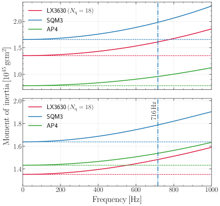
Figure 16: The upper panel shows the relation between the moment of inertia and spin frequency for constant central density sequence. We take the central mass-energy to be $7.67\times 10^{14}\,\rm g\,cm^{-3}$, which corresponds to $M=1.4M_{\odot}$ for the EoS LX3630 ($N_{\rm q}=18$). The solid lines are the moment of inertia for rotating stars $I+\delta I$, while the dashed lines represent the moment of inertia for non-rotating configuration $I$. The lower panel shows the moment of inertia in the constant baryonic mass sequence. We take the baryonic mass as $1.67\,M_{\odot}$, which corresponds to the gravitational mass $M=1.4\,M_{\odot}$ for the EoS LX3630 ($N_{\rm q}=18$). The solid lines represent $I+\delta I$ while the dashed lines represent $I$. The vertical line at $716\,\rm Hz$ represents the observed fastest rotating pulsar, PSR J1748$-$2446ad.

In Fig. 16, we plot the moment of inertia versus the rotating frequencies for the constant central density sequence (upper panel) and the constant baryonic mass sequence (lower panel). The constant central density sequence can be represented as simple quadratic functions directly. For low spin, the correction to the moment of inertia is very tiny. In the case of PSR J0737$-$3039A, the rotating frequency is $\sim 45.5\,\rm Hz$ and the second order contribution can be ignored in the discussions of Lense-Thirring precession. But the corrections become obvious as the star rotates sufficiently fast. For example, for PSR J1748$-$2446ad, the fastest spinning pulsar observed with the frequency $716\,\rm Hz$, the relative error $\delta I/(I+\delta I)$ one makes by neglecting the contribution $\delta I$ at order $\Omega^{2}$ are $8.8\%$ for LX3630 ($N_{\rm q}=18$), $8.3\%$ for SQM3, and $6.8\%$ for AP4. In Table 1, we present the relative errors for the constant baryonic mass sequence shown in the lower panel of Fig. 16 at different rotating frequencies. The relative errors for LX3630 and SQM3 are larger than AP4, which results from the fact that SSs and QSs are more compact than hadronic NSs.

Table 1: The relative error $\delta I/(I+\delta I)$ for EoSs LX3630 ($N_{\rm q}=18$), SQM3, and AP4 in different rotating frequencies.

	Relative errors $\delta I/(I+\delta I)\,[\%]$
Frequency $\,[\rm Hz]$	LX3630	SQM3	AP4
100	$0.197$	$0.191$	$0.149$
200	$0.792$	$0.755$	$0.577$
300	$1.77$	$1.67$	$1.28$
400	$3.08$	$2.91$	$2.26$
500	$4.68$	$4.41$	$3.47$
600	$6.50$	$6.13$	$4.91$
700	$8.48$	$8.01$	$6.54$
800	$10.6$	$10.0$	$8.34$
900	$12.7$	$12.0$	$10.3$
1000	$15.0$	$14.0$	$12.3$

5 Tidal deformation and tidal Love numbers

For tidally-deformed relativistic stars, the metric $g_{tt}$ in the star’s local asymptotical rest frame can be represented via (Flanagan & Hinderer, 2008; Hinderer, 2008)

$$-\frac{\left(1+g_{tt}\right)}{2}= -\frac{M}{r}-\frac{3Q_{ij}}{2r^{3}}\left(n^{i}n^{j}-\frac{1}{3}\delta^{ij}\right)+O\left(\frac{1}{r^{4}}\right)$$

$$+\frac{1}{2}\mathcal{E}_{ij}x^{i}x^{j}+O\left(r^{3}\right)\,,$$ (62)

where $\mathcal{E}_{ij}$ is the tidal field generated by the companion of the star, and $Q_{ij}$ is the quadrupole moment of the NS induced by the tidal field. To characterize the deformations of the stars, one usually defines the tidal deformability as

$$\lambda\equiv-Q_{ij}/\mathcal{E}_{ij}\,,$$ (63)

which measures the ability to be deformed by the tidal field and depends on the EoS. It is related to the $l=2$ Love number $k_{2}$ via $k_{2}=3\lambda R^{-5}/2$.

To calculate the metric in Eq. (5) and give the tidal deformability $\lambda$, one introduces a $l=2$ even parity and static perturbation on the spherical background. The metric perturbation in the Regge-Wheeler gauge (Regge & Wheeler, 1957) can be represented as (Thorne & Campolattaro, 1967)

$$h_{\mu\nu}^{(2m)}=Y_{2m}(\theta,\phi)\left[\begin{matrix}-e^{\nu}H_{0}&H_{1}&0&0\\ H_{1}&e^{\lambda}H_{2}&0&0\\ 0&0&\rho^{2}K&0\\ 0&0&0&\rho^{2}\sin^{2}\theta K\end{matrix}\right]\,,\\$$ (64)

where $Y_{lm}(\theta,\phi)$ are the spherical harmonics and $H_{0}$, $H_{1}$, $H_{2}$ and $K$ are functions that only depend on $r$. Correspondingly, the matter perturbations are

$$\delta T^{0}_{0}=-\delta\rho(r)Y_{20}(\theta,\phi)\,,\quad\delta T_{i}^{i}=\delta P(r)Y_{20}(\theta,\varphi)\,.$$ (65)

Substituting $\delta P$ into $\delta\rho\,{\rm d}P/{\rm d}\rho$ and solving the linearized Einstein equations, $\delta G^{\beta}_{\alpha}=8\pi T^{\beta}_{\alpha}$, one obtains (Hinderer, 2008; Damour & Nagar, 2009)

$$H_{0}=-H_{2}=H\,,\quad H_{1}=0\,,\quad K^{\prime}=-H^{\prime}-H\nu^{\prime}\,,$$ (66)

where the prime denotes the derivative respect to $r$. The ordinary differential equations of $H(r)$ and $\alpha(r)\equiv H^{\prime}(r)$ are

$$\frac{{\rm d}H}{{\rm d}r}= \alpha(r)\,,$$ (67)

$$\frac{{\rm d}\alpha}{{\rm d}r}= -\alpha(r)\left\{\frac{2}{r}+e^{\lambda}\left[\frac{2m(r)}{r^{2}}+4\pi r(P-\rho)\right]\right\}$$

$$-H\left[-\frac{6e^{\lambda}}{r^{2}}+4\pi e^{\lambda}\left(5\rho+9P+\frac{\rho+P}{{\rm d}P/{\rm d}\rho}\right)-\nu^{\prime 2}\right]\,.$$ (68)

One integrates the differential equations of $H(r)$ and $\alpha(r)$ to the surface of the star $R$ with the boundary conditions $H(r)=ar^{2}$ and $\alpha(r)=2ar$ as $r\rightarrow 0$. Here $a$ is a constant that can be chosen arbitrarily and will be cancelled in the calculations of the Love numbers. For QSs and SSs, the term ${\rm d}P/{\rm d}\rho$ in the differential equation of $\alpha$ is not continuous across the surface of the star, just like the case in the slow rotation. Thus, the match conditions of $H(r)$ and $\alpha(r)$ at the radius $R$ is

$$[H]=0\,,\quad[\alpha]=[H^{\prime}]=-4\pi r^{2}H(R_{-})\rho(R_{-})/M\,.$$ (69)

The exterior solution of $H$ can be solved analytically (Thorne & Campolattaro, 1967; Hinderer, 2008)

$$H=c_{1}Q_{2}^{2}\left(\frac{r}{M}-1\right)+c_{2}P_{2}^{2}\left(\frac{r}{M}-1\right)\,,$$ (70)

where $c_{1}$ and $c_{2}$ are constants. The function $P_{2}^{2}$ is the associated Legendre function of the first kind and $P_{2}^{2}(r/M-1)\sim r^{2}$ at large $r$, while the function $Q_{2}^{2}$ is the associated Legendre function of the second kind and $Q_{2}^{2}(r/M-1)\sim r^{-3}$ at large $r$. Taking the expansion of $H(r)$ at large $r$ and comparing with the multipole moments defined in Eq. (5), one obtains

$$\lambda=\frac{8M^{5}}{45}\frac{c_{1}}{c_{2}}\,,\quad k_{2}=\frac{3}{2}\lambda R^{-5}=\frac{4\mathcal{C}^{5}}{15}\frac{c_{1}}{c_{2}}\,.$$ (71)

One matches the solutions of $H(r)$ and $\alpha(r)$ at the surface of the star and gives the solutions of $c_{1}/c_{2}$ in terms of the interior solution at $r=R$. Then the tidal Love number $k_{2}$ can be obtained (Hinderer, 2008)

$$k_{2}= \frac{8\mathcal{C}^{5}}{5}(1-2\mathcal{C})^{2}[2+2{\mathcal{C}}(y-1)-y]$$

$$\times\Big{\{}2{\mathcal{C}}[6-3y+3{\mathcal{C}}(5y-8)]$$

$$+4{\mathcal{C}}^{3}\left[13-11y+{\mathcal{C}}(3y-2)+2\mathcal{C}^{2}(1+y)\right]$$

$$+3(1-2\mathcal{C})^{2}[2-y+2\mathcal{C}(y-1)]\ln(1-2\mathcal{C})\Big{\}}^{-1}\,,$$ (72)

where $y\equiv R\alpha(R)/H(R)$. For QSs or SSs, one needs to take into account the match conditions in Eq. (69), and $y(R)$ can be represented as

$$y(R)=\frac{R\alpha(R_{-})}{H(R_{-})}-\frac{4\pi R^{3}\rho({R_{-})}}{M}\,.$$ (73)

The second term contributes crucially to the tidal Love numbers of QSs or SSs and cannot be ignored. The tidal deformability can be calculated with the relation $\lambda=2k_{2}R^{5}/3$. For later analysis of GW constraints, we will concentrate on the dimensionless tidal deformability

$$\Lambda=\frac{2k_{2}}{3\mathcal{C}^{5}}\,.$$ (74)

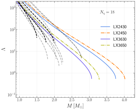
Figure 17: Dimensionless tidal deformability $\Lambda$ as a function of the mass $M$ for SSs ($N_{\rm q}=18$), QSs (black dashed lines), and normal NSs (grey dashed lines). For SSs with $N_{\rm q}=9$, the trend of $\Lambda$ is basically the same as $N_{\rm q}=18$, and we do not show them here for clarity.

In Fig. 17, we display the relation between the dimensionless tidal deformabilities and the masses for SSs, QSs, and normal NSs. For the mass range we plot, a common feature is that $\Lambda$ decreases with the increase of the mass because the star becomes more and more compact and harder to be deformed. For SSs, as the potential depth $\epsilon$ increases and the surface baryonic density $n_{\rm s}$ decreases, the EoS becomes stiffer, which leads to larger maximal masses and tidal deformabilities. Compared to normal NSs and QSs, SSs are very compact near the maximal masses and the dimensionless tidal deformabilities can extend to the value smaller than one. For Schwarzschild black holes, the tidal deformabilities are zero since $1-2\mathcal{C}$ in Eq. (5) becomes zero. This feature is guaranteed by the no hair theorem (Damour & Nagar, 2009).

One can notice that tidal deformability is proportional to the fifth power of the radius $R$. Therefore, constraining or measuring tidal deformability of NSs can provide important information on the EoS of NSs. Actually, the tidal deformations of NSs have imprints on the GWs from binary NSs. At the early stage of inspiral, the dynamical motion can be treated as point particles. But once the binary system evolves to the late stage of inspiral, the finite size effects induced by the tidal interactions will affect the motions of binary system and contribute to the GW emission (Flanagan & Hinderer, 2008). The tidal contributions to the evolution of GW phases first enter at 5 PN. It is actually a Newtonian term in spite of scaling with PN order. Since the energy goes to deform the star and the induced quadrupole moments will contribute to the GW radiation, the phase evolution will be faster than non-spinning point particles with the same mass (Dietrich et al., 2021). The phase corrections depend on a parameter $\tilde{\Lambda}$, which is a mass-weighted linear combination of the dimensionless tidal deformabilities of two stars (Flanagan & Hinderer, 2008)

$$\tilde{\Lambda}=\frac{16}{13}\frac{\left(m_{1}+12m_{2}\right)m_{1}^{4}\Lambda_{1}+\left(m_{2}+12m_{1}\right)m_{2}^{4}\Lambda_{2}}{\left(m_{1}+m_{2}\right)^{5}}\,,$$ (75)

where $m_{1,2}$ and $\Lambda_{1,2}$ represent the masses and the tidal deformabilities of the binary components respectively.

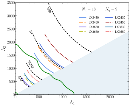
Figure 18: Posterior of tidal deformabilities (green lines) for the binary NS in GW170817 with restricted low spins. The data of the posterior is taken from Abbott et al. (2019). The green line indicates the enclosure of the $90\%$ credible regions of $\tilde{\Lambda}$, $300_{-230}^{+420}$. The primary mass $m_{1}\in(1.36,1.60)\,{M}_{\odot}$ and the secondary mass $m_{2}\in(1.16,1.36)\,{M}_{\odot}$. The tidal deformability for SSs with $N_{\rm q}=18$ and $N_{\rm q}=9$ are displayed. For comparison, we also plot the tidal deformabilities for AP4, H4, MS0, and SQM3. The shaded region is $\Lambda_{1}>\Lambda_{2}$.

The GWs from the binary NS inspiral, GW170817, give the constraints on the tidal deformabilities for the first time  (Abbott et al., 2017, 2018, 2019). In the discovery paper, Abbott et al. (2017) placed a $90\%$ upper limit of $\tilde{\Lambda}\leq 800$ for low spin prior. With a linear expansion of $\Lambda(m)$ at fiducial mass $1.4\,M_{\odot}$, they also gave $\Lambda(1.4M_{\odot})\leq 800$. In a following paper, Abbott et al. (2019) extended the range of the GW frequencies from $30\,\rm Hz$ in the initial analysis (Abbott et al., 2017) down to $23\,\rm Hz$. Besides, several sophisticated and more accurate waveform models augmented with other physical effects (such as spins) are used to do data analysis. Under minimal assumptions about the nature of the compact objects, Abbott et al. (2019) constrained the tidal deformability $\tilde{\Lambda}$ in the range $\tilde{\Lambda}\in(0,630)$ for a high spin prior and $\tilde{\Lambda}\in(70,720)$ for a low spin prior. Abbott et al. (2018) complemented the study of Abbott et al. (2019) with the assumptions that GW170817 comes from the inspiral of a binary NS whose masses and spins are consistent with the galactic binaries. They concluded that the tidal deformability for a $1.4\,M_{\odot}$ NS is in the range $\tilde{\Lambda}\in(70,580)$ at a $90\%$ incredible level. For QSs, Miao et al. (2021) used GW170817 data and gave a systematic study with Bayesian inference.

In Fig. 18, we take the posterior in Abbott et al. (2019) and plot the $90\%$ credible lines for the low spin case. This posterior uses minimal assumptions on the nature of the compact objects. The tidal deformabilities for several SSs with $N_{\rm q}=18$ and $N_{\rm q}=9$ are presented. For comparison, we also show some selected models of normal NSs and QSs. The constraints rule out several stiff normal EoSs (MS0, H4) and models of SSs with very low surface baryonic densities (LX2430, LX2450) at a $90\%$ credible level. Recall that the surface baryonic density is inversely proportional to the cubic of $\sigma$. Thus the constraints indicate that the repulsive core cannot extend too large.

Using the posterior of tidal deformabilities in Abbott et al. (2017), Lai et al. (2019) constrained the parameter space of the potential depth $\epsilon$ and surface baryonic density $n_{\rm s}$ for SSs with $N_{\rm q}=18$. Based on their work, we plot the contours for tidal deformabilities and maximal masses for $N_{\rm q}=18$ and $N_{\rm q}=9$ in Fig. 19 and Fig. 20 respectively. If we take the conservative constraint $\Lambda(1.4M_{\odot})\leq 800$ in the initial work (Abbott et al., 2017), the maximal mass at least should be less than $4.2\,M_{\odot}$ in the parameter space we choose.

Figure 19: Contour lines of $\Lambda(1.4M_{\odot})$ (red) and maximal mass (blue) for $N_{\rm q}=18$.

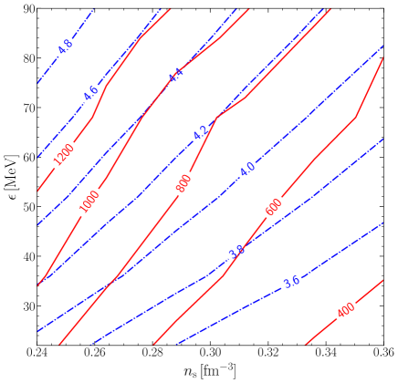
Figure 20: Same as Fig. 19, but for $N_{\rm q}=9$.

6 I-Love-Q universal relations

Yagi & Yunes (2013a, b) found remarkable EoS-insensitive universal relations between the dimensionless moment of inertia $\bar{I}=I/M^{3}$, quadrupole moment $\bar{Q}$, and the tidal deformability $\Lambda$, which is the so-called I-Love-Q universal relations. The relative errors of the analytical fits (Yagi & Yunes, 2013a, 2017) connecting any of two quantities in the I-Love-Q relations hold to $1\%$ for a variety of EoSs, including models for normal NSs and QSs.

The I-Love-Q relations are useful in many aspects. For example, if one obtains the moment of inertia from the aforementioned pulsar timing technique, then an accurate estimation of the rotational quadrupole moment $\bar{Q}$ can be made. The eccentricity, quadrupole moment, and moment of inertia affect the modelling of the X-ray profiles of pulsars (Morsink et al., 2007; Bauböck et al., 2013a; Bauböck et al., 2013b; Gao et al., 2020). The finite size effects from rotation and tidal interactions will contribute to the continuous GW emission (Hinderer, 2008; Yagi & Yunes, 2013a; Harry & Hinderer, 2018; Dietrich et al., 2021). Therefore, the I-Love-Q relations can be used to break degeneracies between some parameters in the modelling of X-ray profiles and waveform of GWs (Yagi & Yunes, 2013a, 2017; Bauböck et al., 2013b; Silva & Yunes, 2018). In this way, the parameter space can be reduced and other parameters in the modelling can be obtained more accurately (Yagi & Yunes, 2017; Bauböck et al., 2013b).

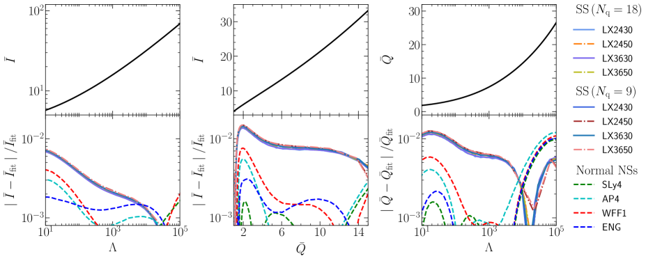
Figure 21: The EoS-insensitive universal relations between dimensionless quantities $\bar{I}$, $\bar{Q}$, and $\Lambda$. The quantities are normalized via $\bar{I}\equiv I/M^{3}$, $\bar{Q}\equiv-Q_{\mathrm{r}}/(M^{3}\chi^{2})$, and $\Lambda\equiv\lambda/M^{5}$. Here $M$ is the mass of the non-rotating configuration, $\chi=J/M^{2}$ is the dimensionless spin, and $J$ is the angular momentum in the first order of $\Omega$. In the first row, we show the fitting curves of I-Love-Q relations taken from Yagi & Yunes (2017). In the second row, we show the relative errors between the fitting values and the numerical data for SSs and normal NSs.

So far, we have calculated static, slowly rotating, and tidally deformed SSs. Compared to other kinds of EoSs, SSs in the Lennard-Jones model admits ${\rm d}P/{\rm d}\rho>1$ with the causality still being satisfied. Therefore, it is worthwhile to see whether the I-Love-Q universal relations still hold for SSs. Yagi & Yunes (2013a, 2017) showed that the I-Love-Q relations can be fitted by fifth-order polynomials in the form

$$\ln y_{i}=\sum_{k=0}^{4}c_{k}\left(\ln x_{i}\right)^{k}\,,$$ (76)

with great accuracy. Here $y_{i}$ and $x_{i}$ are any two quantities in $\bar{I}$, $\bar{Q}$, and $\Lambda$, and $c_{k}$ are fitting coefficients. In the first row of Fig. 21, we show the fitting curves with the fitting constants $c_{k}$ given in Yagi & Yunes (2017). In the second row, we show the relative errors between the fitting values and the numerical data. For SS, the relative errors are smaller than $1\%$ for SSs in the most regions of the parameter space. Some departures occur in the $\bar{I}$-$\bar{Q}$ and $\bar{Q}$-$\Lambda$ relations, but the relative errors are still in the order of $1\%$. We come to the conclusion that the I-Love-Q relations still hold despite ${\rm d}P/{\rm d}\rho>1$.

Another interesting feature is that the relative errors of SSs are nearly the same for the EoS models that we choose. An instinctive reason is that the EoS models come from the same form of mathematical equations (the Lennard Jones model). We can further understand this feature (at least for the $\bar{I}$–$\bar{Q}$ relation) with the eccentricities of those stars. After the discovery of the I-Love-Q relations, Yagi et al. (2014) explored the reason why this universality occurs. They suggested that the universality results from an emergent approximate symmetry. With the increase of the compactness, the variation of the eccentricity defined in Eq. (4.2) inside stars decreases, which leads to a self-similarity of the isodensity surface inside of the stars. This self-similarity indicates some common matter distributions, therefore the universal behavior occurs for the exterior multipole moments. Motivated by this argument, In Fig. 22, we plot the eccentricities inside of the stars $e(r)$ divided by the surface eccentricity $e_{\rm s}$ for different choices of parameters. We can notice that the variations of eccentricities at given radial coordinate are very narrow for the selected models, about $1.8$–$3.8\%$. The values and the range of the variations of eccentricities are much smaller than that of different normal NSs used in the analysis of Yagi et al. (2014). Therefore, if we use this scenario of how the universality occurs, the features with nearly the same relative errors for SSs can be understood, at least for the $\bar{I}$–$\bar{Q}$ relation.

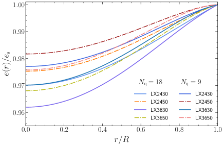
Figure 22: The eccentricity $e(r)$ at a given isodensity surface inside of the SSs divided by the eccentricity at the star’s surface $e_{\rm s}$. Here we choose $M=1.4\,M_{\odot}$ and relations for $N_{\rm q}=18$ and $N_{\rm q}=9$ are displayed.

In above discussions, we only consider slow rotation. For rapidly rotating NSs, Doneva et al. (2013) extended the computation of the $\bar{I}$–$\bar{Q}$ relation to the mass shedding limit and found that the universality is lost. Chakrabarti et al. (2014) discovered that it is still universal among various EoSs if one uses some dimensionless parameters to characterize the magnitude of rotation. More interestingly, one of the parameters involves the radius of NSs and a new universal relation expressing the radius with mass and spin parameter was found, which can be used as a powerful tool for radius measurement. Pappas & Apostolatos (2014) discovered that the first four multipoles of NSs are related in a way that is independent of the EoS of NSs, which let us describe the geometry around NSs with only a few parameters quite accurately. Because of the ultra-compact nature, the universal relations and spacetime geometry of rapidly rotating SSs may give us more valuable information. We leave them to future study.

7 Discussions and Conclusions

Bulk strong matter at several times of nuclear densities may restore the three-light-flavor symmetry (Xu, 2003, 2018). At this energy level, the quarks may not be deconfined and form quark clusters, which we call strangeons. The residual strong interactions can trap the strangeons in the potential well and the whole star is in a solid state. Therefore, we conjecture that the pulsar-like compact objects could be actually SSs rather than NSs or QSs. We use the Lennard-Jones model, which is parametrized by the potential depth $\epsilon$ and the surface baryonic density $n_{\rm s}$, to describe the EoS of SSs. Though simple, it provides a powerful physically motivated framework to study strangeon stars, complementing the parametrization usually seen for NSs (Read et al., 2009). In the Lennard-Jones model, the EoS is very stiff due to the non-relativistic nature of the particles and the strong repulsive force between the strangeons in the short distance. The astronomical observations may give certain constraints on the parameters and even verify or falsify the existence of SSs. Thus, we calculate the static, slowly rotating, and tidally deformed SSs in details and briefly discuss some existing and possible future observations that can constrain the EoS of SSs. The results in this work are ready to be used in various scenarios.

In the calculations of the static and non-spinning background, all the parameter space in our model can produce maximal mass $M_{\rm max}$ larger than $2.5\,M_{\odot}$. In our model, ultra-compact stars near the maximal mass can invade into the region ${\rm d}P/{\rm d}\rho>1$ with the causality limit still being satisfied. We also compared the structures of SSs with the analytical Tolman IV and Tolman VII solutions discussed in Tolman (1939), Lattimer & Prakash (2005), and Lattimer (2012). We found that the SSs can possess maximal mass larger than the ones given by Tolman VII solution but is still lower than that of Tolman IV solution. If pulsar-like compact stars are SSs, a much long-lived star will form in the remnant of the GW170817 event (Lai et al., 2019). A stiffer EoS predicts smaller central mass-energy density at maximal mass. If future observations of the shapiro time delay with pulsar timing technique and post-merger signals from binary mergers support the existence of massive pulsar-like compact objects with mass larger than $2.5\,M_{\odot}$, the phase transition from hadrons to free quarks may not happen and the existence of SSs is favored.

For slowly rotating SSs, we calculated the structures to the third order of angular frequency $\Omega$. In the first order, the star remains to be spherical and the local inertial frame is dragged. We calculated the angular momentum $J$ and the moment of inertia $I$ of SSs and some representative models of normal NSs and QSs. Based on the work of Lattimer & Prakash (2001) and Bejger & Haensel (2002), we studied the universal relations between the moment of inertia and the compactness of the star. At low compactness, this universal relation for SSs is basically the same as QSs. But as the compactness becomes larger, EoS of QSs becomes soft while SSs are still very stiff. The universal relation will deviate from QSs and the moment of inertia is always close to the limit set by the incompressible fluid. The frame dragging effect will induce Lense-Thirring precession in the double pulsar system PSR J0737$-$3039A/B. The periastron advance due to the spin-orbit coupling may be detectable in the upcoming years with the SKA (Hu et al., 2020). A $10\%$ precision of the moment-of-inertia measurement can give informative constraints on the parameter space of $\epsilon$ and $n_{\rm s}$ in our model.

To the order $\Omega^{2}$, the star is deformed. On the spherical part, we calculated the spherical stretching and the change in gravitational mass and the baryonic mass. Differently from NSs, SSs have a hard surface with finite density. The match conditions at the surface of star cannot be ignored and the corrections must be crucially considered. On the quadrupole part, we calculated the quadrupole moments, eccentricities of isodensity surface, and investigated the universal relation between the dimensionless quadrupole moments and compactness discussed by Urbanec et al. (2013). We found similar features shown in the relations between the moment of inertia and the compactness. At large compactness, the relations for SSs deviate from QSs. We also find quasi-universal relations between the surface eccentricity and the compactness for SSs, QSs, and normal NSs. The relations basically have the same features as the relations between the quadrupole moments and the compactness. We also found that the eccentricity and the compactness for SSs and QSs satisfy quasi-universal relations, which are distinct from the relation for normal NSs shown in Bauböck et al. (2013b).

To the third order of $\Omega$, we studied the corrections to the angular momentum and the moment of inertia for the constant central density sequence and the constant baryonic mass sequence. We found that for moderate spins, the corrections of moment of inertia $\delta I$ are very small compared to the zeroth-order contribution $I$. But for rapidly rotating stars, the corrections can be up to $\sim 10\%$ for the EoSs we considered. For rapidly rotating NSs, Benhar et al. (2005) found that the relative errors of the perturbative approach compared to the results calculated from numerical relativity can be reduced largely if the third order contributions are considered. This conclusion could also be used for SSs. Our calculations may be useful to study the spin evolutions of newly-born SSs or glitch processes in pulsars.

For the tidally deformed SSs, we calculated the tidal deformabilities with the appropriate match conditions at the surface of the stars. We used the posterior of GW170817 to give a constraint on the parameter space of $\epsilon$ and $n_{\rm s}$. If we take the constraint of $\Lambda(1.4\,M_{\odot})\leq 800$ (Abbott et al., 2017), we then come to the conclusion that the maximal mass cannot be larger than $\sim 4.2\,M_{\odot}$ both for $N_{\rm q}=18$ and $N_{\rm q}=9$. In the future, smaller values of $\Lambda(1.4{M_{\odot}})$ are expected.

Based on the calculations of slow rotation and tidal deformation, we studied the I-Love-Q universal relations (Yagi & Yunes, 2013a, b). The universal relations still hold although ${\rm d}P/{\rm d}\rho>1$. We also discussed the nearly the same relative errors compared to the fitting formula given in Yagi et al. (2014) especially for the $\bar{I}$-$\bar{Q}$ relation. The I-Love-Q relations and other universal relations such as the $I$-$\mathcal{C}$ and $\bar{Q}$-$\mathcal{C}$ relations can be used to study the GWs from the binaries and the modelling of X-ray profiles.

A main concern of our calculations is that we take the perfect fluid assumption to calculate the perturbations but SSs are actually in a solid state. The key parameter for the calculations of the perturbations for solid components is the shear modulus $\mu$. For NSs, the structure can be roughly divided into a superdense fluid core and a solid crust. The interactions in the crust are dominated by electromagnetic force and the mean shear modulus in the crust is about $\mu\simeq 4\times 10^{29}\,\rm erg/cm^{3}$ (Ushomirsky et al., 2000; Owen, 2005). Penner et al. (2011) developed a framework to study the tidal response of NSs with solid crusts. They found that the elasticity of the solid crust provides a small correction to the tidal deformability. Recently, Gittins et al. (2020) presented detailed formalism that describes the static perturbations on the relativistic NSs with solid crust and corrected some inconsistencies in Penner et al. (2011). The results shows that the inclusion of the solid crust has a negligible effect on the tidal deformability of a NS, in the range of $\sim 10^{-8}$–$10^{-7}$.

However, in our model, the interactions between strangeons are dominated by strong force. The detailed calculations of the shear modulus is still not performed, but it should be much larger than that of the NS’s crust. If the burst oscillation frequencies observed in low-mass X-ray binaries correspond to the first few torsional modes of SSs, the shear modulus should be about one thousand times of the NS’s crust, say $\mu\simeq 4\times 10^{32}\,\rm erg/cm^{3}$ (Xu, 2003; Owen, 2005). We do not know how large the tidal deformability will deviate from the fluid case for SSs, but we can obtain some key insights of this problem from the calculations of tidal deformabilities for crystalline color superconducting phase (Lau et al., 2017, 2019). QSs composed of crystalline color superconducting phase are rigid with extremely high shear modulus (Alford et al., 2001; Mannarelli et al., 2007). The shear modulus is approximately given by (Mannarelli et al., 2007)

$$\mu=2.47\,\mathrm{MeV}/\mathrm{fm}^{3}\left(\frac{\Delta}{10\,\mathrm{MeV}}\right)^{2}\left(\frac{\mu_{\rm q}}{400\,\mathrm{MeV}}\right)^{2}\,,$$ (77)

where $\mu_{\rm q}$ is the average quark chemical potential and $\Delta$ is the gap parameter which is in the range of $5$–$25\,\rm MeV$. If the shear modulus is taken to be $\mu=4\times 10^{32}\,\rm erg/cm^{3}$ ($\Delta\simeq 5\,\rm MeV$), according to the results in Lau et al. (2017, 2019), the deviations of the tidal deformabilities from the fluid case are in the order of $1\%$. For larger gap parameters, the deviations can be very large and more interestingly, they found that the universal relations between the moment of inertia and tidal deformability will deviate from the ones for fluid stars. If we take the shear modulus to be about $\mu\simeq 4\times 10^{32}\,\rm erg/cm^{3}$, the corrections may not be very large and the results discussed in our work is a good approximation. But if the shear modulus is actually larger, then we need to consider the corrections due to the elasticity.

For the slow rotation approximation, Carter & Quintana (1975) developed Hartle-Thorne approximation and gave the method to construct an elastic rotational solid star  based on the elastic perturbation theory in general relativity (Carter, 1973; Andersson & Comer, 2021). To the first order of $\Omega$, the star remains to be spherical and Quintana (1976) found that the moment of inertia is the same as that of fluid case. For higher order perturbations, the star will be deformed and one needs to consider the effects of solid state. The deviations to the fluid cases are also determined by the value of shear modulus, which may have the same order of effects as the tidal. Anyway, we ignore the solid aspects, namely the shear modulus, of the stars in this study. In future, we will present the calculations of the shear modulus and use the elastic perturbations in general relativity to study the structures of SSs.

The nature of the supra-nuclear matter in compact stars closely relates to the non-perturbative QCD at low energy levels, which still remains to be an unsolved important problem in physics. The proposed SSs perceive pulsar-like compact objects as solid stars composed of strangeons. We give a study on the structures of rotating and tidally-deformed SSs within a perturbative approach. So far, the SSs have passed many tests. The future observations of X-rays, radio signals, and GWs will give us more information on the SSs and the bulk of strong matter at low energy scales.

Data Availability

The data underlying this paper will be shared on reasonable request to the corresponding authors.

Appendix A Ordinary differential equations related to slowly rotating relativistic stars

The metric for slowly rotating relativistic star to the third order of $\Omega$ can be represented as

$${\rm d}s^{2}= \left\{-e^{\nu(r)}\left[1+2\big{(}h_{0}+h_{2}P_{2}(\cos\theta)\big{)}\right]+r^{2}\omega^{2}\sin^{2}\theta\right\}{\rm d}t^{2}$$

$$+e^{\lambda(r)}\left[1+2\big{(}m_{0}+m_{2}P_{2}(\cos\theta)\big{)}/\big{(}r-2m\big{)}\right]{\rm d}r^{2}$$

$$+r^{2}\left[1+2(v_{2}-h_{2})P_{2}(\cos\theta)\right]\left({\rm d}\theta^{2}+\sin^{2}\theta{\rm d}\phi^{2}\right)$$

$$-2r^{2}\sin^{2}\theta\left[\omega+w_{1}-\frac{1}{\sin\theta}\frac{{\rm d}P_{3}(\cos\theta)}{{\rm d}\theta}w_{3}\right]{\rm d}\phi{\rm d}t$$

$$-4r^{2}\sin^{2}\theta P_{2}(\cos\theta)\big{(}v_{2}-h_{2}\big{)}\omega{\rm d}\phi{\rm d}t\,.$$ (78)

Combining this metric with the stress-energy tensor in Eq. (26) and applying the linearized Einstein equations, a systematic ordinary differential equations which determine the stars’ structures can then be obtained.

In the following, we will give these differential equations, the boundary conditions at the center of the star, and the match conditions between the interior and the exterior solutions order by order. Most of the equations can be found in Hartle (1967); Hartle & Thorne (1968); Hartle (1973); Chandrasekhar & Miller (1974); Benhar et al. (2005); Urbanec et al. (2013). Note that some typos in the original work (Hartle, 1967) have been corrected.

A.1 The first order

To the first order of $\Omega$, the star remains to be spherical and only the spacetime is dragged due to the rotation of the star. The fluid motion is not determined by the angular velocity $\Omega$ relative to a distant observer but by the angular velocity $\bar{\omega}$ with respect to the local inertial frame, which is defined as

$$\bar{\omega}=\Omega-\omega\,.$$ (79)

This quantity satisfies the differential equation

$$\frac{1}{r^{4}}\frac{{\rm d}}{{\rm d}r}\left(r^{4}j\frac{{\rm d}\bar{\omega}}{{\rm d}r}\right)+\frac{4}{r}\frac{{\rm d}j}{{\rm d}r}\bar{\omega}=0\,,$$ (80)

where $j=e^{-(\nu+\lambda)/2}$. In practice, we follow Sumiyoshi et al. (1999) and Benhar et al. (2005) and introduce two variables

$$\xi=j\bar{\omega}\,,\quad u=r^{4}j\frac{{\rm d}\bar{\omega}}{{\rm d}r}\,,$$ (81)

which satisfy

$$\frac{{\rm d}\xi}{{\rm d}r}=\frac{u}{r^{4}}-\frac{4\pi r^{2}(\rho+P)\xi}{r-2m}\,,\quad\frac{{\rm d}u}{{\rm d}r}=\frac{16\pi r^{5}(\rho+P)\xi}{r-2m}\,,$$ (82)

in the interior of the star. The boundary conditions of $\xi$ and $u$ at the center of the star are

$$\xi(0)=j_{\rm c}\bar{\omega}_{\rm c}\,,\quad u(0)=0\,,$$ (83)

where $j_{\rm c}$ and $\bar{\omega}_{\rm c}$ are the values of $j$ and $\bar{\omega}$ at the center of the star. Integrating Eq. (82) with the boundary conditions at the center of the star, one obtains the interior solutions. Outside of the star, the stress-energy tensor $T_{\alpha\beta}$ vanishes and the solutions of Eq. (82) are

$$\xi(r)=\Omega-\frac{2J}{r^{3}}\,,\quad u(r)=6J\,,$$ (84)

where $J$ is the angular momentum of the star. Taking the matching conditions at the surface of the star

$$[\xi]=0\,,\quad[u]=0\,,$$ (85)

the angular momentum $J$, angular velocity $\Omega$, and the moment of inertia $I$ can be represented as

$$J=u(R)/6\,,\quad\Omega=\xi(R)+\frac{2J}{R^{3}}\,,\quad I\equiv J/\Omega\,.$$ (86)

A.2 The second order

To the order $\Omega^{2}$, the stars will be deformed and the perturbations can be divided into $l=0$ and $l=2$ parts in the spherical harmonics expansions, which correspond to spherical stretching and quadrupole deformations respectively. The isodensity surface at radial coordinate $r$ in the non-rotating configuration is displaced to

$$r+\xi_{0}(r)+\xi_{2}(r)P_{2}(\cos\theta)\,,$$ (87)

in the rotating configuration. The displacement functions $\xi_{0}$ and $\xi_{2}$ can be represented as

$$\xi_{0}(r)=-p_{0}(\rho+P)/(\mathrm{d}P/\mathrm{d}r)\,,\quad\xi_{2}(r)=-p_{2}(\rho+P)/(\mathrm{d}P/\mathrm{d}r)\,,$$ (88)

where $p_{0}$ and $p_{2}$ are related to the metric perturbation via

$$p_{0}= -h_{0}+\frac{r^{3}\xi^{2}}{3(r-2m)}+h_{0\rm c}\,,$$ (89)

$$p_{2}= -h_{2}-\frac{r^{3}\xi^{2}}{3(r-2m)}\,,$$ (90)

where $h_{0\rm c}$ is a constant. The above two equations can also be treated as the definitions of $p_{0}$ and $p_{2}$.

A.2.1 Spherical part

The spherical part of the perturbations can be obtained by integrating the differential equations of the “mass perturbation factor” $m_{0}$ and the “pressure perturbation factor” $p_{0}$

$$\frac{{\rm d}m_{0}}{{\rm d}r}= \frac{u^{2}}{12r^{4}}+\frac{8\pi r^{5}(\rho+P)\xi^{2}}{3(r-2m)}+4\pi r^{2}(\rho+P)\frac{{\rm d}\rho}{{\rm d}P}p_{0}\,,$$ (91)

$$\frac{{\rm d}p_{0}}{{\rm d}r}= \frac{u^{2}}{12r^{4}(r-2m)}+\frac{2r^{2}\xi}{3(r-2m)}\left[\frac{u}{r^{3}}+\frac{r-3m-4\pi r^{3}P}{r-2m}\xi\right]$$

$$-\frac{(1+8\pi r^{2}P)m_{0}}{(r-2m)^{2}}-\frac{4\pi r^{2}(\rho+P)p_{0}}{r-2m}\,.$$ (92)

In practice, one can integrate the equations with the boundary conditions at $r\rightarrow 0$

$$m_{0}(r)= \frac{4\pi}{15}\big{(}\rho_{\rm c}+P_{\rm c}\big{)}\left[\frac{{\rm d}\rho}{{\rm d}P}\mid_{r=0}+2\right]\xi(0)^{2}r^{5}\,,$$ (93)

$$p_{0}(r)= \frac{1}{3}\xi(0)^{2}r^{2}\,.$$ (94)

where $\rho_{\rm c}$ and $P_{\rm c}$ are the energy density and the pressure at the center of the star. Outside of the star, the analytical solution of $m_{0}$ is

$$m_{0}(r)=\delta M-\frac{J^{2}}{r^{3}}\,.$$ (95)

The constant $\delta M$ is the correction of the gravitational mass at order $\Omega^{2}$. The match condition of $m_{0}$ at surface of the star is

$$[m_{0}]=\frac{4\pi R^{3}\rho\left(R_{-}\right)(R-2M)p_{0}(R)}{M}\,.$$ (96)

Then the total gravitational mass of the rotating star can be represented as

$$M+\delta M=M+m_{0}(R)+\frac{J^{2}}{R^{3}}+\frac{4\pi R^{3}\rho\left(R_{-}\right)(R-2M)p_{0}(R)}{M}\,.$$ (97)

Once $p_{0}$, $\delta M$ and $J$ are calculated, the interior solution of $h_{0}$ can be obtained from Eq. (89), while the exterior solution of $h_{0}$ is

$$h_{0}(r)=-\frac{\delta M}{r-2M}+\frac{J^{2}}{r^{3}(r-2M)}\,.$$ (98)

The spherical stretching of isodensity surface at the radial coordinate $r$ can be represented as

$$\xi_{0}(r)=p_{0}r(r-2m)\Big{/}\left(m+4\pi r^{3}P\right)\,,$$ (99)

and the variation of the stellar radius $\delta R$ is then

$$\delta R=\xi_{0}(R)=\frac{R(R-2M)p_{0}(R)}{M}\,.$$ (100)

A.2.2 Quadrupole part

We obtain the quadrupole deformation of the star by integrating the differential equations of $h_{2}$ and $v_{2}$

$$\frac{{\rm d}v_{2}}{{\rm d}r}= \frac{1}{r(r-2m)}\bigg{\{}-2h_{2}\left(m+4\pi r^{3}P\right)+\big{(}r-m+4\pi r^{3}P\big{)}$$

$$\times\left[\frac{8\pi r^{5}(\rho+P)\xi^{2}}{3(r-2m)}+\frac{u^{2}}{6r^{4}}\right]\bigg{\}}\,,$$ (101)

$$\frac{{\rm d}h_{2}}{{\rm d}r}= h_{2}\Bigg{\{}\frac{r^{2}}{2\left(m+4\pi r^{3}P\right)}\left[8\pi(\rho+P)-\frac{4m}{r^{3}}\right]-\frac{2\left(m+4\pi r^{3}P\right)}{r(r-2m)}\Bigg{\}}$$

$$-\frac{2v_{2}}{m+4\pi r^{3}P}+\frac{u^{2}}{6r^{5}}\left[\frac{m+4\pi r^{3}P}{r-2m}-\frac{r}{2\left(m+4\pi r^{3}P\right)}\right]$$

$$+\frac{8\pi r^{5}(\rho+P)\xi^{2}}{3(r-2m)}\left[\frac{m+4\pi r^{3}P}{r(r-2m)}+\frac{1}{2\left(m+4\pi r^{3}P\right)}\right]\,.$$ (102)

The general interior solutions of $h_{2}$ and $v_{2}$ can be obtained by combinations of homogeneous solutions and particular solutions,

$$v_{2}=v_{2}^{\rm p}+C\,v_{2}^{\rm h}\,,\quad h_{2}=h_{2}^{\rm p}+C\,h_{2}^{\rm h}\,,$$ (103)

where $C$ is a constant to be determined. The particular solutions $v_{2}^{\rm p}$ and $h_{2}^{\rm p}$ can be calculated by integrating Eqs. (A.2.2–A.2.2) and taking the boundary conditions near the center of the star

$$v_{2}^{\rm p}=Br^{4}\,,\quad h_{2}^{\rm p}=Ar^{2}\,.\\$$ (104)

The constants $A$ and $B$ satisfy

$$B+2\pi\big{(}\frac{1}{3}\rho_{\rm c}+P_{\rm c}\big{)}A=\frac{2\pi}{3}\left(\rho_{\rm{c}}+P_{\rm{c}}\right)\xi(0)^{2}\,.$$ (105)

The homogeneous solutions $v_{2}^{\rm h}$ and $h_{2}^{\rm h}$ can be obtained by integrating

$$\frac{{\rm d}v_{2}^{\rm h}}{{\rm d}r}= \frac{1}{r(r-2m)}\left\{-2h_{2}^{\rm h}\left(m+4\pi r^{3}P\right)\right\}\,,$$ (106)

$$\frac{{\rm d}h_{2}^{\rm h}}{{\rm d}r}= h_{2}^{\rm h}\Bigg{\{}\frac{r^{2}}{2\left(m+4\pi r^{3}P\right)}\left[8\pi(\rho+P)-\frac{4m}{r^{3}}\right]-\frac{2\left(m+4\pi r^{3}P\right)}{r(r-2m)}\Bigg{\}}$$

$$-\frac{2v_{2}^{\rm h}}{m+4\pi r^{3}P}\,,$$ (107)

with the boundary conditions at $r\rightarrow 0$

$$v_{2}^{\rm h}=B_{1}r^{4}\,,\quad h_{2}^{\rm h}=A_{1}r^{2}\,.$$ (108)

The constants $A_{1}$ and $B_{1}$ satisfy the relation

$$B_{1}+2\pi\Big{(}\frac{1}{3}\rho_{\rm c}+P_{\rm c}\Big{)}A_{1}=0\,.$$ (109)

The exterior solutions of $v_{2}$ and $h_{2}$ can be calculated analytically

$$h_{2}= J^{2}\left(\frac{1}{Mr^{3}}+\frac{1}{r^{4}}\right)+KQ_{2}^{2}\left(\frac{r}{M}-1\right)\,,$$ (110)

$$v_{2}= -\frac{J^{2}}{r^{4}}+K\frac{2M}{[r(r-2M)]^{1/2}}Q_{2}^{1}\left(\frac{r}{M}-1\right)\,,$$ (111)

where $Q_{2}^{1}$ and $Q_{2}^{2}$ are Legendre functions of the second kind and $K$ is a constant to be determined together with $C$ by matching the interior and exterior solutions at the boundary of the star. The match conditions are

$$[v_{2}]=0\,,\quad[h_{2}]=0\,.$$ (112)

The quadrupole moment can then be read off from the Newtonian potential far from the star

$$Q=-\frac{8KM^{3}}{5}-\frac{J^{2}}{M}\,.$$ (113)

The function $m_{2}$ can be obtained from an algebraic relation

$$m_{2}=(r-2m)\left[-h_{2}+\frac{8\pi r^{5}(\epsilon+P)\xi^{2}}{3(r-2m)}+\frac{u^{2}}{6r^{4}}\right]\,,$$ (114)

and the match condition at the surface of the star is

$$[m_{2}]=-8\pi R^{5}\rho(R_{-})\xi(R)^{2}/3$$ (115)

Once we know the solutions of $v_{2}$, $h_{2}$ and $m_{2}$, the function $p_{2}$ can be calculated from the relation in Eq. (90). The eccentricity of the isodensity surface can be defined as (Hartle & Thorne, 1968)

$$e(r)=\left[-3\left(v_{2}-h_{2}+\xi_{2}/r\right)\right]^{1/2}\,,$$ (116)

and the surface eccentricity $e_{\rm s}$ can be obtained by taking $r=R$.

A.3 The third order

In the third order, the $l=1$ function $w_{1}$ and the $l=3$ function $w_{3}$ will enter. As we mentioned in the main text, the correction to the angular momentum and moment of inertia do not depend on the function $w_{3}$. Therefore, we only concentrate on the calculation of $w_{1}$. The differential equation is (Hartle, 1973; Benhar et al., 2005)

$$\frac{{\rm d}}{{\rm d}r}\left(r^{4}j\frac{{\rm d}w_{1}}{{\rm d}r}\right)+4r^{3}\frac{{\rm d}j}{{\rm d}r}w_{1}=r^{4}D_{0}-\frac{1}{5}r^{4}D_{2}\,,$$ (117)

where

$$r^{4}D_{0}= -u\frac{{\rm d}}{{\rm d}r}\left[\frac{m_{0}}{r-2m}+h_{0}\right]-\frac{16\pi r^{5}\xi(\rho+P)}{r-2m}$$

$$\times\left[\frac{2m_{0}}{r-2m}+(\frac{{\rm d}\rho}{{\rm d}P}+1)p_{0}+\frac{2r^{3}\xi^{2}}{3(r-2m)}\right]\,,$$ (118)

$$\frac{r^{4}D_{2}}{5}= \frac{u}{5}\frac{{\rm d}}{{\rm d}r}\left[4v_{2}-5h_{2}-\frac{m_{2}}{r-2m}\right]-\frac{16\pi r^{5}\xi(\rho+P)}{r-2m}$$

$$\times\left[\frac{2m_{2}}{r-2m}+(\frac{{\rm d}\rho}{{\rm d}P}+1)p_{2}-\frac{2r^{3}\xi^{2}}{3(r-2m)}\right]\,.$$ (119)

Similarly with the first order, we introduce two variables

$$\xi_{1}=jw_{1}\,,\quad u_{1}=r^{4}j\frac{{\rm d}w_{1}}{{\rm d}r}\,,$$ (120)

and Eq. (117) can then be written as

$$\frac{{\rm d}\xi_{1}}{{\rm d}r}= \frac{u_{1}}{r^{4}}-\frac{4\pi r^{2}(\rho+P)\xi_{1}}{r-2m}\,,$$ (121)

$$\frac{{\rm d}u_{1}}{{\rm d}r}= \frac{16\pi r^{5}(\rho+P)\xi_{1}}{r-2m}+r^{4}D_{0}-\frac{r^{4}}{5}D_{2}\,.$$ (122)

Inside of the star, the general solutions are combinations of particular solutions and homogeneous solutions

$$\xi_{1}=\xi_{1}^{\rm p}+C_{1}\,\xi_{1}^{\rm h}\,,\quad u_{1}=u_{1}^{\rm p}+C_{1}\,u_{1}^{\rm h}\,,$$ (123)

where $C_{1}$ is a constant. The particular solutions can be obtained with the boundary conditions at the center of the star

$$\xi_{1}^{\rm p}(0)=0\,,\quad u_{1}^{\rm p}(0)=0\,.$$ (124)

Setting $D_{0}=D_{2}=0$, one obtains the homogeneous equations. The solutions of $\xi_{1}^{\rm h}$ and $u_{1}^{\rm h}$ can be obtained by integrating the homogeneous equations with the asymptotical conditions at $r\rightarrow 0$

$$\xi_{1}^{\rm h}(r)= A_{2}\left[1-\frac{2\pi}{5}\big{(}\rho_{\rm c}+P_{\rm c}\big{)}r^{2}\right]\,,$$ (125)

$$u_{1}^{\rm h}(r)= A_{2}\left[\frac{16\pi}{5}\big{(}\rho_{\rm c}+P_{\rm c}\big{)}r^{5}\right]\,,$$ (126)

where $A_{2}$ is a constant that can be chosen arbitrarily. Outside of the star, $\xi_{1}$ and $u_{1}$ can be solved analytically

$$\xi_{1}(r)=\frac{2\delta J}{r^{3}}+G(r)\,,\quad u_{1}(r)=-6\delta J+Y(r)\,.$$ (127)

The functions $G(r)$ and $Y(r)$ can be represented as (Benhar et al., 2005)

$$G(r)= -\frac{12J^{3}}{5r^{7}}-\frac{4J^{3}}{5Mr^{6}}+\frac{JK}{40M^{3}r^{4}}\bigg{[}108r^{4}\ln\left(\frac{r}{r-2M}\right)$$

$$-288r^{3}M\ln\left(\frac{r}{r-2M}\right)+33r^{4}-240r^{3}M$$

$$+336r^{2}M^{2}+256M^{3}r-96M^{4}$$

$$+192rM^{3}\ln\left(\frac{r}{r-2M}\right)+12r^{4}\ln\left(\frac{r}{r-2M}\right)\bigg{]}-\frac{33JK}{40M^{3}}\,,$$ (128)

$$Y(r)= \frac{84J^{3}}{5r^{4}}+\frac{24J^{3}}{5Mr^{3}}+\frac{24KJQ_{2}^{2}\big{(}\frac{r}{M}-1\big{)}}{5}-\frac{48KMJQ^{1}_{2}\big{(}\frac{r}{M}-1\big{)}}{5\big{(}r(r-2M)\big{)}^{1/2}}\,.$$ (129)

The constant $\delta J$ is the angular momentum at order $\Omega^{3}$, which can be obtained together with $C_{1}$ by matching the solutions of $\xi_{1}$ and $u_{1}$ at the boundary of the star. Note that the match conditions of $\xi_{1}$ and $u_{1}$ are

$$[\xi_{1}]= 0\,,$$ (130)

$$[u_{1}]= -\frac{16\pi R^{6}\rho\left(R_{-}\right)\xi(R)}{M}\left(p_{0}(R)-\frac{1}{5}p_{2}(R)\right)$$

$$-\frac{4\pi R^{3}\rho(R_{-})u(R)p_{0}(R)}{M}-\frac{8\pi R^{5}\rho(R_{-})u(R)\xi(R)^{2}}{15(R-2M)}\,.$$ (131)

The contribution of the moment of inertia at the second order of $\Omega$ is $\delta I=\delta J/\Omega$.

References

- Abbott et al. (2017) Abbott B. P., et al., 2017, PhRvL, 119, 161101
- Abbott et al. (2018) Abbott B. P., et al., 2018, PhRvL, 121, 161101
- Abbott et al. (2019) Abbott B. P., et al., 2019, PhRvX, 9, 011001
- Alcock et al. (1986) Alcock C., Farhi E., Olinto A., 1986, ApJ, 310, 261
- Alford et al. (2001) Alford M. G., Bowers J. A., Rajagopal K., 2001, PhRvD, 63, 074016
- Alford et al. (2008) Alford M. G., Schmitt A., Rajagopal K., Schäfer T., 2008, RvMP, 80, 1455
- Andersson & Comer (2021) Andersson N., Comer G. L., 2021, LRR, 24, 3
- Antoniadis et al. (2013) Antoniadis J., et al., 2013, Sci, 340, 448
- Barker & O’Connell (1975) Barker B. M., O’Connell R. F., 1975, PhRvD, 12, 329
- Bauböck et al. (2013a) Bauböck M., Psaltis D., Ozel F., 2013a, ApJ, 766, 87
- Bauböck et al. (2013b) Bauböck M., Berti E., Psaltis D., Özel F., 2013b, ApJ, 777, 68
- Baym et al. (2018) Baym G., et al., 2018, RPPh, 81, 056902
- Bejger & Haensel (2002) Bejger M., Haensel P., 2002, A&A, 396, 917
- Benhar et al. (2005) Benhar O., Ferrari V., Gualtieri L., Marassi S., 2005, PhRvD, 72, 044028
- Berti & Stergioulas (2004) Berti E., Stergioulas N., 2004, MNRAS, 350, 1416
- Berti et al. (2005) Berti E., White F., Maniopoulou A., Bruni M., 2005, MNRAS, 358, 923
- Bludman & Ruderman (1968) Bludman S. A., Ruderman M. A., 1968, PhRv, 170, 1176
- Bogdanov et al. (2008) Bogdanov S., Grindlay J. E., Rybicki G. B., 2008, ApJ, 689, 407
- Burgay et al. (2003) Burgay M., et al., 2003, Natur, 426, 531
- Caporaso & Brecher (1979) Caporaso G., Brecher K., 1979, PhRvD, 20, 1823
- Caporaso & Brecher (1983) Caporaso G., Brecher K., 1983, PhRvD, 28, 2694
- Carter (1973) Carter B., 1973, CMaPh, 30, 261
- Carter & Quintana (1975) Carter B., Quintana H., 1975, ApJ, 202, 511
- Chakrabarti et al. (2014) Chakrabarti S., et al., 2014, PhRvL, 112, 201102
- Chandrasekhar & Miller (1974) Chandrasekhar S., Miller J. C., 1974, MNRAS, 167, 63
- Damour & Nagar (2009) Damour T., Nagar A., 2009, PhRvD, 80, 084035
- Damour & Schaefer (1988) Damour T., Schaefer G., 1988, NCimB, 101, 127
- Demorest et al. (2010) Demorest P., et al., 2010, Natur, 467, 1081
- Dietrich et al. (2021) Dietrich T., Hinderer T., Samajdar A., 2021, GReGr, 53, 27
- Doneva et al. (2013) Doneva D. D., et al., 2013, ApJL, 781, L6
- Ellis et al. (2007) Ellis G., Maartens R., MacCallum M. A. H., 2007, GReGr, 39, 1651
- Farhi & Jaffe (1984) Farhi E., Jaffe R. L., 1984, PhRvD, 30, 2379
- Flanagan & Hinderer (2008) Flanagan E. E., Hinderer T., 2008, PhRvD, 77, 021502
- Fonseca et al. (2021) Fonseca E., et al., 2021, ApJL, 915, L12
- Gao et al. (2020) Gao Y., Shao L., Xu R., Sun L., Liu C., Xu R.-X., 2020, MNRAS, 498, 1826
- Gittins et al. (2020) Gittins F., Andersson N., Pereira J. P., 2020, PhRvD, 101, 103025
- Harry & Hinderer (2018) Harry I., Hinderer T., 2018, CQGra, 35, 145010
- Hartle (1967) Hartle J. B., 1967, ApJ, 150, 1005
- Hartle (1973) Hartle J. B., 1973, Ap&SS, 24, 385
- Hartle & Sharp (1967) Hartle J. B., Sharp D. H., 1967, ApJ, 147, 317
- Hartle & Thorne (1968) Hartle J. B., Thorne K. S., 1968, ApJ, 153, 807
- Hinderer (2008) Hinderer T., 2008, ApJ, 677, 1216
- Hu et al. (2020) Hu H., et al., 2020, MNRAS, 497, 3118
- Ishii et al. (2007) Ishii N., Aoki S., Hatsuda T., 2007, PhRvL, 99, 022001
- Isoyama et al. (2018) Isoyama S., Nakano H., Nakamura T., 2018, PTEP, 2018, 073E01
- Jones (1924) Jones J. E., 1924, RSPSA, 106, 463
- Kasen et al. (2017) Kasen D., et al., 2017, Natur, 551, 80
- Kasliwal et al. (2017) Kasliwal M., et al., 2017, Sci, 358, 1559
- Kramer & Wex (2009) Kramer M., Wex N., 2009, CQGra, 26, 073001
- Lackey et al. (2006) Lackey B. D., Nayyar M., Owen B. J., 2006, PhRvD, 73, 024021
- Lai & Xu (2009a) Lai X.-Y., Xu R.-X., 2009a, APh, 31, 128
- Lai & Xu (2009b) Lai X.-Y., Xu R.-X., 2009b, MNRAS, 398, 31
- Lai & Xu (2017) Lai X.-Y., Xu R.-X., 2017, J. Phys. Conf. Ser., 861, 012027
- Lai et al. (2018a) Lai X.-Y., et al., 2018a, RAA, 18, 024 (Paper I)
- Lai et al. (2018b) Lai X.-Y., et al., 2018b, MNRAS, 476, 3303
- Lai et al. (2019) Lai X.-Y., Zhou E.-P., Xu R.-X., 2019, EPJA, 55, 60
- Lai et al. (2020) Lai X.-Y., et al., 2020, arXiv e-prints, p. arXiv:2009.06165
- Lattimer (2012) Lattimer J. M., 2012, ARNPS, 62, 485
- Lattimer & Prakash (2001) Lattimer J. M., Prakash M., 2001, ApJ, 550, 426
- Lattimer & Prakash (2005) Lattimer J. M., Prakash M., 2005, PhRvL, 94, 111101
- Lattimer & Schutz (2005) Lattimer J. M., Schutz B. F., 2005, ApJ, 629, 979
- Lau et al. (2017) Lau S. Y., Leung P. T., Lin L. M., 2017, PhRvD, 95, 101302
- Lau et al. (2019) Lau S. Y., Leung P. T., Lin L. M., 2019, PhRvD, 99, 023018
- Liu & Shao (2021) Liu C., Shao L., 2021, arXiv e-prints, p. arXiv:2108.08490
- Lu et al. (2018) Lu J.-G., Zhou E.-P., Lai X.-Y., Xu R.-X., 2018, SCPMA, 61, 089511
- Lu et al. (2019) Lu J.-G., et al., 2019, SCPMA, 62, 959505
- Machleidt (2001) Machleidt R., 2001, PhRvC, 63, 024001
- Mannarelli et al. (2007) Mannarelli M., Rajagopal K., Sharma R., 2007, PhRvD, 76, 074026
- Miao et al. (2021) Miao Z., Jiang J.-L., Li A., Chen L.-W., 2021, ApJL, 917, L22
- Michel (1991) Michel F. C., 1991, NuPhS, 24, 33
- Miller et al. (2019) Miller M. C., et al., 2019, ApJL, 887, L24
- Misner et al. (1973) Misner C. W., Thorne K. S., Wheeler J. A., 1973, Gravitation. W. H. Freeman, San Francisco
- Morsink et al. (2007) Morsink S. M., Leahy D. A., Cadeau C., Braga J., 2007, ApJ, 663, 1244
- Owen (2005) Owen B. J., 2005, PhRvL, 95, 211101
- Pappas & Apostolatos (2014) Pappas G., Apostolatos T. A., 2014, PhRvL, 112, 121101
- Penner et al. (2011) Penner A. J., et al., 2011, PhRvD, 84, 103006
- Poisson (1998) Poisson E., 1998, PhRvD, 57, 5287
- Quintana (1976) Quintana H., 1976, ApJ, 207, 279
- Read et al. (2009) Read J. S., et al., 2009, PhRvD, 79, 124032
- Regge & Wheeler (1957) Regge T., Wheeler J. A., 1957, PhRv, 108, 1063
- Reina (2016) Reina B., 2016, MNRAS, 455, 4512
- Reina et al. (2017) Reina B., Sanchis-Gual N., Vera R., Font J. A., 2017, MNRAS, 470, L54
- Rhoades & Ruffini (1974) Rhoades Jr. C. E., Ruffini R., 1974, PhRvL, 32, 324
- Riley et al. (2019) Riley T. E., et al., 2019, ApJL, 887, L21
- Ruderman (1968) Ruderman M., 1968, PhRv, 172, 1286
- Shao (2019) Shao L., 2019, AIP Conf. Proc., 2127, 020016
- Shao et al. (2015) Shao L., et al., 2015, PoS, AASKA14, 042
- Shao et al. (2017) Shao L., et al., 2017, PhRvX, 7, 041025
- Shapiro & Teukolsky (1983) Shapiro S. L., Teukolsky S. A., 1983, Black holes, white dwarfs, and neutron stars: the physics of compact objects. Wiley-VCH
- Silva & Yunes (2018) Silva H. O., Yunes N., 2018, CQGra, 35, 015005
- Stergioulas (2003) Stergioulas N., 2003, LRR, 6, 3
- Stoks et al. (1994) Stoks V. G. J., et al., 1994, PhRvC, 49, 2950
- Sumiyoshi et al. (1999) Sumiyoshi K., Ibáñez J. M., Romero J. V., 1999, A&AS, 134, 39
- Thorne & Campolattaro (1967) Thorne K. S., Campolattaro A., 1967, ApJ, 149, 591
- Thorne & Hartle (1984) Thorne K. S., Hartle J. B., 1984, PhRvD, 31, 1815
- Tolman (1939) Tolman R. C., 1939, PhRv, 55, 364
- Urbanec et al. (2013) Urbanec M., Miller J. C., Stuchlik Z., 2013, MNRAS, 433, 1903
- Ushomirsky et al. (2000) Ushomirsky G., Cutler C., Bildsten L., 2000, MNRAS, 319, 902
- Walecka (1974) Walecka J., 1974, AnPhy, 83, 491
- Wang et al. (2017) Wang W.-Y., et al., 2017, ApJ, 837, 81
- Wang et al. (2020) Wang W.-Y., et al., 2020, MNRAS, 500, 5336
- Watts et al. (2016) Watts A. L., et al., 2016, RvMP, 88, 021001
- Weber & Glendenning (1991) Weber F., Glendenning N. K., 1991, in International Summer School on Nuclear Astrophysics.
- Weber & Glendenning (1992) Weber F., Glendenning N. K., 1992, ApJ, 390, 541
- Weltman et al. (2020) Weltman A., et al., 2020, PASA, 37, e002
- Wilczek (2007) Wilczek F., 2007, Natur, 445, 156
- Wiringa et al. (1995) Wiringa R. B., Stoks V. G. J., Schiavilla R., 1995, PhRvC, 51, 38
- Witten (1984) Witten E., 1984, PhRvD, 30, 272
- Xu (2003) Xu R.-X., 2003, ApJL, 596, L59
- Xu (2009) Xu R.-X., 2009, JPhG, 36, 064010
- Xu (2018) Xu R.-X., 2018, SCPMA, 61, 109531
- Xu & Guo (2017) Xu R.-X., Guo Y.-J., 2017, Strange Matter: A State before Black Hole. World Scientific Publishing, pp 119–146
- Xu et al. (1999) Xu R.-X., Qiao G.-J., Zhang B., 1999, ApJL, 522, L109
- Yagi & Yunes (2013a) Yagi K., Yunes N., 2013a, PhRvD, 88, 023009
- Yagi & Yunes (2013b) Yagi K., Yunes N., 2013b, Sci, 341, 365
- Yagi & Yunes (2017) Yagi K., Yunes N., 2017, PhR, 681, 1
- Yagi et al. (2014) Yagi K., et al., 2014, PhRvD, 90, 063010
- Zhou et al. (2004) Zhou A.-Z., Xu R.-X., Wu X.-J., Wang N., 2004, APh, 22, 73
- Zhou et al. (2014) Zhou E.-P., Lu J.-G., Tong H., Xu R.-X., 2014, MNRAS, 443, 2705