In quantum materials, electrons that have strong correlations tend to localize, leading to quantum spins as the building blocks for low-energy physics ^{1, 2}. When strongly correlated electrons coexist with more weakly-correlated conduction electrons, multiple channels of effective interactions develop and compete with each other. The competition creates quantum fluctuations having a large spectral weight, with the associated entropies reaching significant fractions of $R\ln 2$ per electron. Advancing a framework to understand how the fluctuating local moments influence unconventional superconductivity ^{3, 4, 5} is both pressing and challenging. Here we do so in the exemplary setting of heavy-fermion metals, where the amplified quantum fluctuations manifest in the form of Kondo destruction and large-to-small Fermi-surface fluctuations. These fluctuations lead to unconventional superconductivity whose transition temperature is exceptionally high relative to the effective Fermi temperature, reaching several percent of the Kondo temperature scale. Our results provide a natural understanding of the enigmatic superconductivity in a host of heavy-fermion metals. Moreover, the qualitative physics underlying our findings and their implications for the formation of unconventional superconductivity apply to a variety of highly correlated metals with strong Fermi surface fluctuations ^{6, 7}.

E-mail: ^∗qmsi@rice.edu

Strong correlations drive a plethora of quantum phases ^{1, 2}. Heavy-fermion systems represent a prototype of strongly correlated metals ^{8, 9}. Here, the $f$ electrons have a Coulomb repulsion much larger than their kinetic energy, and at low energies they act as quantum spins. The spins are coupled to the $spd$-based conduction electrons by an antiferromagnetic (AF) exchange, the Kondo interaction, and a Ruderman-Kittel-Kasuya-Yosida (RKKY) interaction between the spins that is typically AF as well. The Kondo interaction promotes a ground state with a nonzero amplitude for a collective spin singlet between the local moments and conduction electrons. The Kondo energy scale acts as an effective Fermi energy for the composite fermions, the reincarnation of the local moments that are fractionalized as a result of their inter-locking with the charge-carrying conduction electrons. Unconventional superconductivity develops in about 50 heavy-fermion superconductors, in many cases close to an AF-ordered phase. Examples include CeRhIn₅, which is a part of the Ce-115 materials family with $T_{c}\approx 2.3$ K (a record high among $4f$-electron-based heavy-fermion systems), and CeCu₂Si₂, which has $T_{c}\approx 0.6$K and is the very first unconventional superconductor ever discovered. These transition temperatures are exceptionally high, recognizing that their ratio to the respective effective Fermi temperature is a few percent. This is to be contrasted with what happens in conventional superconductors, where the ratio is typically orders of magnitude smaller.

There is ample empirical evidence that strong correlations, in the form of the Kondo effect, are key to the development of heavy-fermion superconductivity. The amount of entropy involved in the superconducting condensation is a sizeable fraction of R$\ln$2 per electron, implying that spin-$\frac{1}{2}$ local moments are active agents for the superconductivity. A host of spectroscopic measurements support this perspective ³. With a few exceptions ^{10, 11}, the Kondo effect has not been incorporated into theoretical studies of the mechanism of unconventional heavy-fermion superconductivity.

What has been especially lacking is a framework for how unconventional superconductivity develops out of heavy-fermion quantum criticality ^{8, 9}, which arises from a dynamical competition between the RKKY and Kondo interactions and has been recognized as a central ingredient of the correlation physics in the normal state. The AF RKKY interactions, which boost spin-singlet correlations among the local moments, weaken the static Kondo-singlet amplitude. This can lead to two types of AF QCPs ^{12, 13, 14}. In one type, the Kondo destruction (KD) QCP, the static amplitude of the Kondo singlet vanishes as the QCP is approached from the paramagnetic side. The $f$ electrons go from being itinerant composite fermions, which participate in the Fermi-surface formation, to being localized in the AF ground state. This large-to-small Fermi-surface reconstruction characterizes a partial Mott (delocalization-localization) transition across the QCP (see Fig. 1), and is a key part of the experimental signatures ^{15, 16, 17, 18, 4}. In the other type of quantum criticality, the Kondo amplitude remains nonzero at the QCP and the heavy quasiparticles undergo a spin density wave (SDW) transition. Given that the immediately adjacent AF order is an SDW formed from the renormalized $f$-electron-based composite quasiparticles, we will refer to this as an SDW${}_{\!{\rm r}}$ QCP to distinguish it from a conventional SDW transition.

Here we address unconventional superconductivity arising from KD and the concomitant delocalization-localization transition of the $f$ electrons. The quantum fluctuations, which have a large spectral weight, are found to yield robust spin-singlet superconductivity, with $T_{c}$ reaching a few percent of the Kondo temperature scale. Although our analysis is focused on a concrete model suitable for heavy-fermion systems, quantum criticality associated with a delocalization-localization transition appears broadly relevant to a variety of other strongly correlated metals ². Possible materials classes in this category include high-temperature cuprate superconductors ⁶, organic charge-transfer salts ⁷, and moiré systems ^{19, 20}.

A canonical microscopic model for heavy-fermion systems is the Anderson lattice model. It describes a single band of conduction electrons hybridizing with strength $V$ with a band of $4f$ electrons that have a strong on-site Hubbard interaction $U$. The large $U$ creates an antiferromagnetic Kondo exchange coupling $J_{K}\propto V^{2}/U$ between local $f$ moments and itinerant conduction electrons. Acting alone, this gives rise to a bare Kondo temperature $T_{K}^{0}$ [$\approx\rho_{0}^{-1}\exp{-(1/\rho_{0}J_{K})}$, with $\rho_{0}$ being the bare conduction-electron density of states at the Fermi energy], below which the local moments are screened by the conduction electrons. The RKKY interaction $I$ acts between the localized magnetic moments. The ratio $\delta\equiv I/T_{K}^{0}$ determines whether the system will order magnetically or develop heavy Fermi liquid behavior. The periodic Anderson Hamiltonian is (see Methods)

$$H_{\mathrm{AL}} = \sum_{i,j,\sigma}t_{ij}(c_{i\sigma}^{{\dagger}}c_{j\sigma}+\mathrm{h.c})+\sum_{i}\left(\epsilon_{f}n_{fi}+Un_{fi\uparrow}n_{fi\downarrow}\right)$$ (1)

$$+ \sum_{i,\sigma}\left(Vc_{i\sigma}^{{\dagger}}f_{i\sigma}+\mathrm{h.c.}\right)+\sum_{i,j,m}I^{m}_{ij}S^{m}_{fi}S^{m}_{fj}\,,$$

where $c_{i\sigma}$ ($f_{i\sigma}$) destroys a conduction ($4f$) electron at lattice site $i$ with spin $\sigma$, while $\epsilon_{f}$ and $U$ are respectively the $f$-level energy and on-site Coulomb repulsion. In addition to a $c$-electron hopping $t_{ij}$ between lattice sites $i,j$, we have explicitly included an RKKY exchange $I^{m}_{ij}$ between Cartesian component $m\in\{x,y,z\}$ of the localized $4f$ moments. We focus on RKKY interactions in the limits of either Ising anistropy ($I^{x}_{ij}=I^{y}_{ij}=0$, $I^{z}_{ij}=I_{ij}$) or full SU(2) symmetry ($I^{m}_{ij}=I_{ij}$). It is also important to distinguish two types of model according to the way in which the “RKKY density of states” $\rho_{I}(\epsilon)\equiv\sum_{\mathbf{q}}\delta(\epsilon-I_{\mathbf{q}})$ increases from its lower edge at $\epsilon=I_{{\bf Q}}$. (Here, $I_{\mathbf{q}}$ is the Fourier transform of $I_{ij}$ and ${\bf Q}$ is the ordering wave vector in the magnetic phase.) In type I models, $\rho_{I}(\epsilon)$ has a jump onset, characteristic of two-dimensional magnetic fluctuations. In type II models, $\rho_{I}(\epsilon)$ instead increases smoothly $\propto\sqrt{\epsilon-I_{{\bf Q}}}$, reflective of three-dimensional magnetic fluctuations. The Anderson lattice model has been studied in a variety of contexts. For quantum phase transitions, the distinction between KD and SDW${}_{\!{\rm r}}$ criticality has been explored through an extended dynamical mean-field theory (EDMFT) approach ^{12, 21}, with the most detailed results obtained for the case of Ising symmetry ^{22, 23, 24, 25}. The quantum critical dynamics of the KD QCP plays an important role in connecting the theory to experiments ²⁶.

In order to permit study of unconventional superconducting pairing, which is necessarily off-site, we here report the first application of a cluster EDMFT (C-EDMFT) ²⁷, which maps $H_{AL}$ to a self-consistently determined two-site quantum cluster model (see Methods and ref. 27 for additional details). We solve the effective cluster model using the numerically exact continuous time quantum Monte Carlo (CT-QMC) method ²⁸ at nonzero temperatures in a form suitable for our purpose ^{29, 30, 31}.

To assess the ability of the C-EDMFT approach to properly capture the quantum critical dynamics, we first consider the type I model in the limit of Ising-anistropic RKKY interactions. We identify a KD QCP, as demonstrated by the phase diagram in Fig. 1(a). Starting from the paramagnetic side, as the tuning parameter $\delta\equiv I/T_{K}^{0}$ is increased, a renormalized Kondo scale $E_{\mathrm{loc}}$ vanishes at the continuous onset of AF order. The suppression of this energy scale implies the destruction of the Kondo resonance—often referred to as composite fermions or simply $f$ fermions—thereby leading to a transformation from a large Fermi surface (incorporating the $f$ fermons) to a small one (excluding the $f$ fermions), as illustrated schematically in Fig. 1(b). At the KD QCP, the temperature dependence of the AF spin susceptibility has a power-law dependence,

$$\chi_{AF}(T)\sim T^{-\alpha}$$ (2)

with a fractional exponent $\alpha_{\mathrm{Ising}}=0.81(4)$ [Fig. 2(a)], and obeys $\omega_{n}/T$ scaling [Fig. 2(b)]. These are essentially the same results as obtained for Ising anisotropy via single-site EDMFT ^{22, 23, 24, 25}, which captures the fractional exponent $\alpha$ in the dynamical spin susceptibility that has been measured by inelastic neutron scattering ²⁶ in Ising-anisotropic CeCu_5.9Au_0.1. The C-EDMFT calculation demonstrates the robustness of the KD QCP in the presence of finite-size corrections, an important finding given that the anomalous dynamical scaling of the spin response is a key signature of this type of QCP.

In the context of unconventional pairing and superconductivity, we expect the spin-flip part of the RKKY interaction to be essential for driving the formation of spin-singlet Cooper pairs ^{30, 32, 33}. Accordingly, we have solved the C-EDMFT equations of the type I model with SU(2) symmetry. Fig. 3(a) shows the inverse of the static lattice spin susceptibility $\chi_{AF}$ obtained at the lowest temperature $T/T_{K}^{0}=0.001$ and the AF transition temperature $T_{N}$, both as functions of the tuning parameter $I/T_{K}^{0}$. It is seen that $T_{N}$ goes continuously to zero at the QCP $I/T_{K}^{0}=I_{c}/T_{K}^{0}\simeq 0.405(5)$, where $\chi_{AF}$ also diverges. This provides evidence that in the SU(2) symmetric case, just as for Ising anisotropy, the zero-temperature transition is second order. The quantum-critical behavior is also of the KD type: At the QCP, $\chi_{AF}$ follows Eq. (2) with a fractional exponent $\alpha_{SU(2)}=0.71(3)$ [Fig. 2(c)], and it obeys an $\omega_{n}/T$ dynamical scaling with the same fractional exponent [Fig. 2(d)]. These properties are similar to the single-site EDMFT solution ³⁴, including the value of the exponent $\alpha$. Our C-EDMFT results demonstrate the robustness of the Kondo-destruction nature of the quantum-critical properties in the normal state of both the Ising and SU(2) limits of the type I model.

We are now in position to study pairing correlations. The pairing susceptibility $\chi_{SC}$ in the spin-singlet channel [see Supplementary Information, Eq. (S15)] diverges, demonstrating a superconducting phase below a transition temperature $T_{c}$. This is illustrated in Fig. 3(b),(c) which plot the $I/T_{K}^{0}$ dependence of $\chi_{SC}$ and the AF order parameter at $T/T_{K}^{0}=0.02$. It is seen that $\chi_{SC}$ diverges as the AF transition is approached from the paramagnetic side, becoming infinite at some $I/T_{K}^{0}<I_{c}/T_{K}^{0}$.

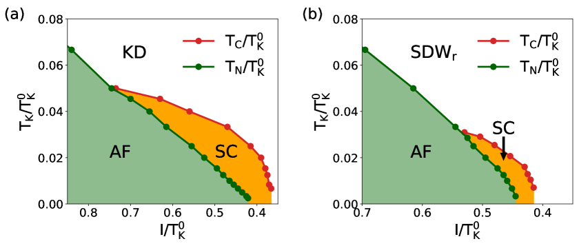
Figure 4: Finite-temperature phase diagram vs control parameter $I/T_{K}^{0}$ for (a) KD and (b) SDW${}_{\!{\rm r}}$ quantum criticality in the SU(2) symmetric case. The transition temperature for the antiferromagnetic (AF) and superconducting (SC) phases is marked by green and red circles, respectively.

We have carried out such calculations at various temperatures and used the location where $\chi_{SC}$ diverges to determine the finite-temperature phase boundary for the superconducting phase. The obtained phase in Fig. 4(a) shows a broad region of superconducting order near to, and indeed hiding, the QCP. The superconducting transition temperature $T_{c}$ reaches a maximum of about 5% of the bare Kondo temperature $T_{K}^{0}$; its value at the QCP is about $0.03T_{K}^{0}$.

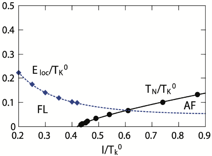
Figure S1: Finite temperature phase diagram vs the ratio of $I/T_{K}^{0}$ for the type-II model with Ising anisotropy. For small $I/T_{K}^{0}$ we find the model is in the FL phase characterized by the static spin susceptibility saturating to a constant for $T\ll E_{\mathrm{loc}}$. For large $I/T_{K}^{0}$ the model develops antiferromagnetic (AF) order. In between the two is the quantum critical non-Fermi liquid regime, where $E_{cr}\equiv E_{\mathrm{loc}}(\delta_{c})$ remains nonzero but is small compared to $T_{K}^{0}$.

We next turn to the second type of quantum critical solution, which we derive in the type II model and is of the SDW${}_{\!{\rm r}}$ type (see Supplementary Information). Here the renormalized Kondo energy scale $E_{\mathrm{loc}}$ does not go to zero upon reaching the QCP from the paramagnetic side. However, $E_{cr}$—the value of $E_{loc}$ at the QCP—is small compared to the bare Kondo energy scale $k_{B}T_{K}^{0}$ (Supplementary Information, Fig. S1). The asymptotic behavior at energies below $E_{cr}$ takes the form of the quantum criticality associated with the conventional SDW QCP ^{35, 36}. The small $E_{cr}/k_{B}T_{K}^{0}$ reflects the considerable reduction of Kondo-singlet correlations due to AF correlations between local moments, and serves to distinguish SDW${}_{\!{\rm r}}$ quantum criticality from conventional SDW QCPs ^{35, 36} where the Kondo effect does not operate.

At an SDW${}_{\!{\rm r}}$ QCP, quantum fluctuations in the intermediate energy range $E_{cr}\lesssim E\lesssim k_{B}T_{K}^{0}$ still manifest the physics of disintegrating Kondo singlets, i.e., the delocalization-localization transition with the Fermi surface crossing over from large to small. These fluctuations will drive unconventional superconductivity along the same lines as at a KD QCP, albeit with a more limited dynamical range and a weaker pairing strength. Indeed, we find that spin-singlet superconductivity develops in the type II model [Fig. 4(b)] with a lower $T_{c}$ than in the type I model ($\simeq 0.02T_{K}^{0}$ at the QCP compared with $0.03T_{K}^{0}$).

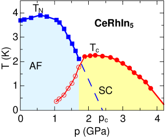
Figure S2: Pressure-temperature phase diagram of CeRhIn₅ at zero magnetic field ^{4, 37}. $T_{N}$ is determined from specific heat measurements. $T_{c}$ is determined from specific heat measurements up to $p=2.5$Gpa and from resistivity measurement at higher pressure.

Our work provides a very general understanding of the superconducting pairing in quantum-critical heavy-fermion metals. We illustrate this point in the context of two prominent examples. The first is CeRhIn₅, which features a pressure-induced QCP ^{4, 37, 9, 38}: As illustrated in Fig. S2, superconductivity develops near the QCP where $T_{c}\approx 2.3$K, which is about 5% of the bare Kondo temperature ($\approx 40$ K; ref. 9). In the magnitude of $T_{c}$ as well as in the spin-singlet nature of the pairing and other properties of its superconducting state, CeRhIn₅ is similar to its high-chemical-pressure counterpart CeCoIn₅ under ambient conditions ³. In both cases, the spin anisotropy is relatively small ⁹, i.e., the SU(2) limit should apply. Importantly, across the critical pressure of CeRhIn₅, quantum oscillation measurements have established a small-to-large Fermi surface jump ^{39, 9}, providing strong evidence for the KD nature of the QCP. Our finding of superconductivity at the KD QCP with a high $T_{c}/T_{K}^{0}$ provides the first theoretical understanding of how superconductivity develops from a strange metal in CeRhIn₅.

A second important material is CeCu₂Si₂, the very first unconventional superconductor observed in nature ⁴⁰. Here, there is considerable experimental evidence that the quantum criticality is of the SDW${}_{\!{\rm r}}$ type, with a crossover temperature $T_{cr}=E_{cr}/k_{B}\approx 1$ K that is small compared to the bare Kondo temperature ($T_{K}^{0}\approx 20$ K). The spin damping rate crosses over from $\propto T^{3/2}$ for $T<T_{cr}$ to $\propto T$ for $T>T_{cr}$ (Ref. 40, 41). Further evidence for the involvement of a $T_{cr}$ that is small compared to $T_{K}^{0}$ has come from an estimate of a change in the kinetic energy across the superconducting transition ⁵. We therefore advance the notion that superconductivity in CeCu₂Si₂ is driven by SDW${}_{\!{\rm r}}$ quantum criticality that sets in below a decade of energies dominated by KD quantum fluctuations.

In our approach, the dynamical competition between the RKKY and Kondo couplings plays a crucial role in capturing the dynamical $\omega/T$ scaling and fractional exponent as well as the small-to-larger Fermi surface transformation in the quantum critical regime, from which the superconducting state develops. This is to be contrasted with other theoretical approaches. One scenario considers multiple channels of conduction ($c$) electrons with the $f$-electron-derived local moments. The multi-channel Kondo effect is suggested to yield a composite $f$-$c$ pairing ¹⁰. Because RKKY interactions are not involved, this picture does not associate the superconductivity with a quantum-critical normal state. An alternative scenario invokes a cluster of local moments self-consistently Kondo-coupled to a conduction-electron bath ¹¹. In this picture, the AF order comes from a static (Hartree-Fock) treatment of RKKY interactions; the lack of dynamical RKKY-Kondo competition also implies the absence of the partial-Mott ($f$-electron delocalization-localization) effect in the normal state.

Taking a wider perspective, we have already noted that a delocalization-localization transition and the accompanying small-to-large Fermi surface transformation have been implicated in a broad range of strongly correlated metals ². These in particular include doped Mott insulators ^{6, 7}, where a rapid change in the carrier concentration has been observed near optimal superconductivity, Analysis of dynamical equations related to the single-site EDMFT analysis of the Kondo lattice has recently been carried out for doped Mott insulators ⁴². It clearly is important to address whether unconventional superconductivity develops in the dynamical equations for such a setting.

To summarize, we have developed a framework to address superconductivity that develops out of a quantum-critical normal state featuring a partial Mott (delocalization-localization) transition and small-to-large Fermi surface transformation. Our theoretical approach captures the critical dynamics in a robust way, and demonstrates superconductivity whose transition temperature is as high as a few percent of the effective Fermi energy. The results provide the first natural understanding of unconventional superconductivity in a variety of prominent families of heavy-fermion materials and offer a promising framework for interpreting superconductivity in other strongly correlated metals such as doped Mott insulators.

Acknowledgments
We would like to thank Gabriel Aeppli, Piers Coleman, Laura H. Greene, Kazushi Kanoda, Stefan Kirchner, Gabriel Kotliar, Silke Paschen, Frank Steglich, Oliver Stockert, Joe D. Thompson, Huiqiu Yuan and Jian-Xin Zhu for useful discussions. This work was supported in part by the National Science Foundation under Grant No. DMR-1920740 (H.H., L.C., and Q.S.) and the Robert A. Welch Foundation Grant No. C-1411 (A.C.). Work at Rutgers University was supported by the Alfred P. Sloan Foundation through a Sloan Research Fellowship (J.H.P.). Computing time was allocated in part by the Data Analysis and Visualization Cyberinfrastructure funded by NSF under grant OCI-0959097 and an IBM Shared University Research (SUR) Award at Rice University, and by the Extreme Science and Engineering Discovery Environment (XSEDE) by NSF under Grants No. DMR170109. J.H.P. acknowledges the hospitality of Rice University. J.H.P., K.I., and Q.S. acknowledge the hospitality of the Aspen Center for Physics, which is supported by the NSF under Grant No. PHY-1607611.

Author contributions The first two authors contributed equally to this work. All authors contributed to the research of the work and the writing of the paper.

Competing interests
The authors declare no competing interests.

Additional information
Correspondence and requests for materials should be addressed to Q.S. (qmsi@rice.edu)

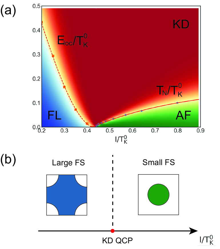
Figure 1: (a) Finite-temperature phase diagram vs $I/T_{K}^{0}$ for type I model. For small $I/T_{K}^{0}$, the model is in a heavy Fermi liquid (FL) phase characterized by the static spin susceptibility saturating to a constant for $T\ll E_{\mathrm{loc}}$. For large $I/T_{K}^{0}$, the model develops antiferromagnetic (AF) order. Between these two regions, in a “fan” above the point where $E_{\mathrm{loc}}$ goes to zero at the QCP, is the quantum critical Kondo destruction (KD) regime of non-Fermi liquid behavior. (b) Schematic reconstruction of the Fermi surface from large to small through the KD QCP. In the quantum critical regime, the Fermi surface fluctuates between the two.

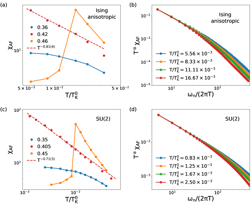
Figure 2: (a) Temperature dependence of $\chi_{AF}$, the static lattice spin susceptibility at the ordering wave vector, and (b) demonstration of $\omega_{n}/T$ scaling for the dynamical lattice spin susceptibility, at the KD QCP in the Ising-anisotropic model. Their counterparts for the SU(2) case are shown in (c) and (d), respectively.

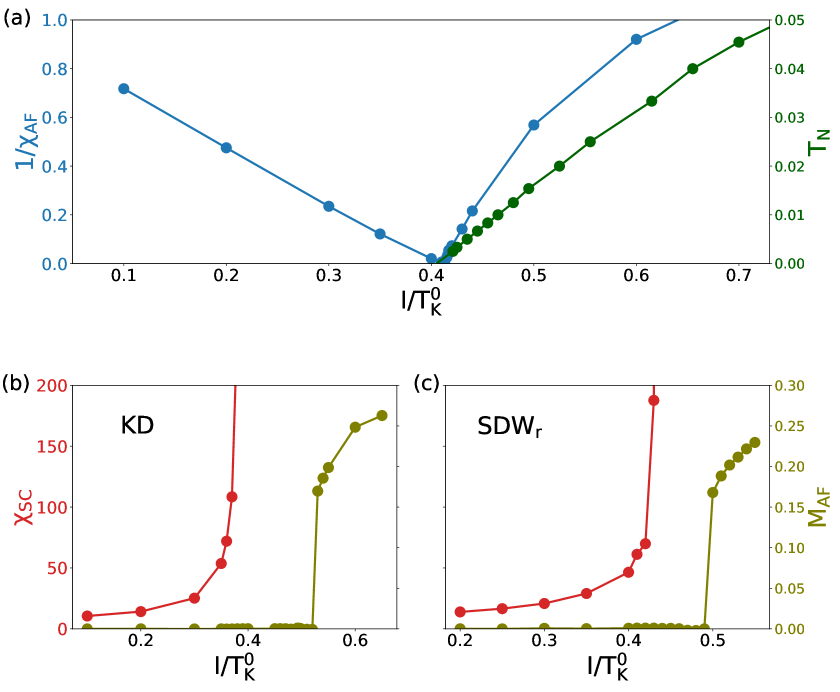
Figure 3: (a) Variation with $I/T_{K}^{0}$ of the inverse static lattice spin susceptibility at the ordering wave vector, $1/\chi_{AF}$, calculated at the lowest accessed temperature $T/T_{K}^{0}=0.001$, and of the AF transition temperature $T_{N}$. (b), (c) Static lattice pairing susceptibility $\chi_{SC}$ and AF order parameter ${M_{AF}}$ vs $I/T_{K}^{0}$ in the type I and type II models, respectively, at a relatively high temperature $T/T_{K}^{0}=0.02$.

Methods

C-EDMFT method   We solve the periodic Anderson model [Eq. (1)] using the C-EDMFT approach of Ref. ²⁷, focusing on a two-site cluster that allows us to study the formation of unconventional Cooper pairs. We iteratively solve the C-EDMFT equations seeking self consistency. In order to achieve reasonably high accuracy, we solve the cluster model at finite temperature using the numerically exact CT-QMC method. Away from the critical regime, the self-consistency loop converges quite fast, within about $30$ iterations. Near the critical point, however, there is a critical slowing down. We find it useful to employ simple mixing techniques ⁴³ to accelerate convergence. Still, the number of iterations can become very large (even exceeding $1000$).

Quantum phase transition   We concentrate on the static spin susceptibility $\chi_{AF}(T)$ at the AF ordering wave vector ${\bf Q}_{\mathrm{AF}}$ (e.g. ${\bf Q}_{\mathrm{AF}}=(\pi/a,\pi/a)$ for a lattice spacing equal to $a$ in two dimensions) and temperature $T$. We mark entry into the antiferromagnetically ordered phase through a diverging $\chi_{AF}$ and a nonzero order parameter $M_{AF}$. To determine the fate of the renormalized Kondo energy scale $E_{\mathrm{loc}}$, we also consider the local spin susceptibility in the AF channel $\chi_{\mathrm{loc}}({\bf Q}_{\mathrm{AF}},i\omega_{n},T)$, where $\omega_{n}=2\pi nk_{B}T/\hbar$ denotes the Matsubara frequency. For zero RKKY interaction, a measure of the effective single ion Kondo temperature $T_{K}^{0}$ can be determined through the inverse of $\chi_{\mathrm{loc}}({\bf Q}_{\mathrm{AF}},i\omega_{n}=0,T=0)$ (see Supplementary Information). The renormalized Kondo energy scale $E_{\mathrm{loc}}$ is related to the dynamical local spin susceptibility (see Supplementary Information and Ref. ¹², ²¹). All spin susceptibilities are measured in units of $(g\mu_{B})^{2}$, where $g$ is the Landé $g$-factor of the local moment and $\mu_{B}$ is the Bohr magneton.

Superconducting instability   To investigate the superconducting instability, we calculate the static pairing susceptibility in the spin-singlet channel $\chi_{SC}(T)$ via a Bethe-Salpeter equation. The superconducting transition temperature is determined by the divergence of the pairing susceptibility $\chi_{SC}(T\rightarrow T_{c})\rightarrow\infty$.

Data availability   The data that support the findings of this study are available from the corresponding author upon reasonable request.

Code availability   The relevant codes used in this study are available from the corresponding author upon reasonable request.

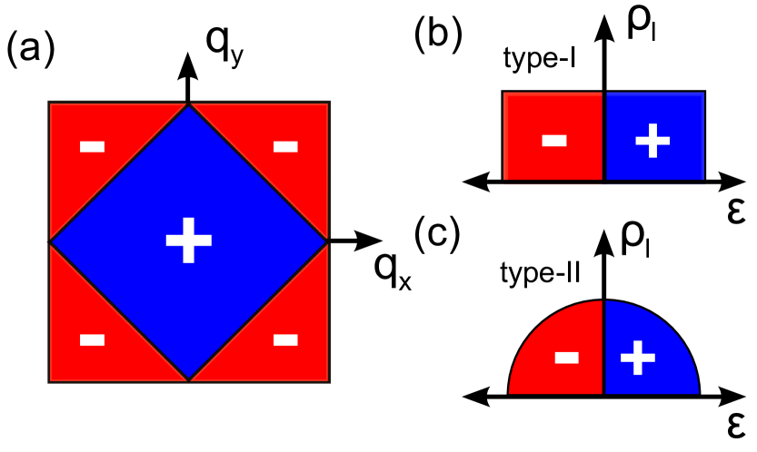
Figure 5: Tiling of the Brillioun zone with the two site cluster (a), where the ferromagnetic fluctuations are confined to the zone center [the blue region (+)] and the antiferromagnetic region at the zone corners [the red region (-)]. The RKKY density of states in the type-I (b) and type-II (c) models are reflective of the two- and three-dimensional magnetic fluctuations.

Supplementary Information

C-EDMFT method   The effective RKKY density of states is defined as follows:

$$\rho_{I}(\epsilon)=\sum_{\mathbf{q}}\delta(\epsilon-I_{\mathbf{q}})$$ (S1)

where $I_{\mathbf{q}}$ is the Fourier transform of $I_{ij}$. Using the two-site cluster, we tile the Brillioun zone so that all ferromagnetic fluctuations are confined to the zone center with cluster momentum ${\bf Q}={\bf Q}_{+}$, and the antiferromagnetic fluctuations on the zone corners with cluster momentum ${\bf Q}={\bf Q}_{-}$, see Fig. 5. In the following we use ${\bf Q}$ and $\tilde{{\bf q}}$ to denote inter and intra cluster momentum respectively and the ordering wavevector is given by ${\bf Q}_{AF}={\bf Q}_{-}$. This tiling of the Brillioun zone leads to a density of states per patch, with $\rho_{I}(\epsilon)=\sum_{\tilde{{\bf q}},{\bf Q}}\delta(\epsilon-I_{\tilde{{\bf q}}+{\bf Q}})=\sum_{{\bf Q}}\rho_{I}({\bf Q},\epsilon)$ and we have defined the density of states in patch ${\bf Q}$.

$$\rho_{I}({\bf Q},\epsilon)=\sum_{\tilde{{\bf q}}}\delta(\epsilon-I_{\tilde{{\bf q}}+{\bf Q}}).$$ (S2)

In the Ising anisotropic case, we choose the cluster momentum in two dimensions ${\bf Q}_{+}=(0,0)$ and ${\bf Q}_{-}=(\pi,\pi)$, as well as ${\bf Q}_{+}=(0,0,0)$ and ${\bf Q}_{-}=(\pi,\pi,\pi)$ in three dimensions (note that the antiferromagnetic ordering wave vector corresponds to ${\bf Q}_{AF}={\bf Q}_{-}$). We set the RKKY interaction $I_{ij}$ to be AF and only consider nearest neighbor interaction, i.e. $I_{q}=I(\cos(q_{x})+\cos(q_{y}))$ for the type I case and $I_{q}=\frac{2}{3}I(\cos(q_{x})+\cos(q_{y})+\cos(q_{z}))$ for the type II case. (We always take $I_{{\bf Q}_{AF}}=-2I$, which serves as our definition for $I$). We approximate the two dimensional density of states with a jump at the lower zone edge. Whereas the three dimensional magnetic density of states vanishes in a square root fashion at the lower zone edge (see Fig. 5).

$$\rho^{\rm type-I}_{I}({\bf Q}_{\pm},\omega) = \frac{1}{2I}\Theta(\pm\omega)\Theta(2I\mp\omega)$$ (S3)

$$\rho^{\rm type-II}_{I}({\bf Q}_{\pm},\omega) = \frac{1}{\pi I^{2}}\Theta(\pm\omega)\Theta(2I\mp\omega)\sqrt{(2I)^{2}-\omega^{2}}$$ (S4)

In the SU(2) case, we also incorporate the next nearest neighbor RKKY interaction. For the type-I case we have $I_{q}=I_{1}(\cos(q_{x})+\cos(q_{y}))+I_{2}(\cos(q_{x}+q_{y})+\cos(q_{x}-q_{y}))$. We choose $I_{1}=-1.5I_{2}>0$ and the cluster momentum ${\bf Q}_{+}=(0,0)$ and ${\bf Q}_{-}=(\pi,\pi)$. For the type II case we have $I_{q}=I_{1}(\cos(q_{x})+\cos(q_{y})\cos(q_{z}))+I_{2}(\cos(q_{x}+q_{y})+\cos(q_{x}-q_{y})+\cos(q_{y}+q_{z})+\cos(q_{y}-q_{z})+\cos(q_{z}+q_{x})+\cos(q_{z}-q_{x}))$. We choose $I_{1}=0.65I_{2}>0$ and the cluster momentum ${\bf Q}_{+}=(0,0,0)$ and ${\bf Q}_{-}=(\pi,\pi,0)$. The ratio of $I_{1}/I_{2}$ is chosen to give us the same value of the RKKY interaction in the cluster, $\bar{I}({\bf Q})$ (defined as $\bar{I}({\bf Q})=2/N\sum_{\tilde{{\bf q}}}I_{\tilde{{\bf q}}+{\bf Q}}$). Again we fix $I_{{\bf Q}_{AF}}=2I$ for both cases.

Here we provide the form of $\rho({\bf Q},\omega)$ we use at only ${\bf Q}_{-}$; for the low-energy behavior, we will only need to keep the bosonic bath at ${\bf Q}={\bf Q}_{-}$.

$$\rho^{\rm type-I}_{I}({\bf Q}{-},\omega) = \frac{\Theta(2I_{2}-\omega)\Theta(2I_{1}+2I_{2}+\omega)}{2I_{1}+4I_{2}}$$ (S5)

$$\rho^{\rm type-II}_{I}({\bf Q}{-},\omega) = \frac{\Theta(\omega-c+r)\Theta(c-\omega)\sqrt{r^{2}-(\omega-c)^{2}}}{\pi r^{2}/4}$$ (S6)

where, for $\rho^{type-II}_{I}$ ,we have used the parameterization $c=2I_{2}$, $r=-2I_{1}+8I_{2}$. They represent the same shape as in equation (S3) (S4) for the Ising case but shifted along the $\epsilon$ axis.

Within the C-EDMFT approach, the single particle and spin self energies depend on cluster momentum ${\bf Q}$, which yields a spin susceptibility

$$\chi(\tilde{{\bf q}}+{\bf Q},i\omega_{n},T)=\frac{1}{I_{\tilde{{\bf q}}+{\bf Q}}+M({\bf Q},i\omega_{n})}.$$ (S7)

To avoid double-counting the RKKY interactions, the conduction electron bath does not become polarized by the finite magnetic order parameter ²⁷. This is achieved by taking a featureless density of states for the conduction band

$$\rho_{c}(\epsilon)=\rho_{0}\Theta(D-|\epsilon|),$$ (S8)

for a half bandwidth $D$ and self-consistently solve for the bosonic baths (see references ^{44, 24, 25} for the one site case). Likewise, because the RKKY interaction is explicitly included (via $I_{ij}$), we drop the dynamic inter-impurity interaction in the lattice model. This is achieved within the effective cluster model, by taking the two impurities to be infinitely far apart ²⁷, and they are then only coupled by $\bar{I}_{{\bf Q}}$ and the bosonic baths. This then corresponds to the cluster Hamiltonian

$$H_{C} = \sum_{i=1,2}H_{AI}^{i}+\sum_{{\bf Q},m}\bar{I}_{{\bf Q}}S^{m}_{{\bf Q},f}S^{m}_{{\bf Q},f}+\sum_{\tilde{{\bf q}},{\bf Q},m}\omega_{\tilde{{\bf q}},{\bf Q}}^{m}\phi^{m{\dagger}}_{\tilde{{\bf q}},{\bf Q}}\phi^{m}_{\tilde{{\bf q}},{\bf Q}}$$ (S9)

$$+ \sum_{\tilde{{\bf q}},{\bf Q},m}g^{m}_{{\bf Q}}(\tilde{{\bf q}})S^{m}_{{\bf Q},f}(\phi^{m{\dagger}}_{\tilde{{\bf q}},{\bf Q}}+\phi^{m}_{-\tilde{{\bf q}},-{\bf Q}})+h_{\mathrm{loc}}S_{{\bf Q},f}^{z}.$$

where ${\bf Q}={\bf Q_{\pm}}$, $\tilde{\bf q}$ run though the momentum points in each patches, and $m=z$ for the ising anisotropic case and $m=x,y,z$ for the SU(2) symmetric case. In the last term, we have included $h_{\mathrm{loc}}=[\delta I_{{\bf Q}_{AF}}+\chi^{z}_{0,-}(i\omega_{n}=0)]\langle S_{{\bf Q}_{AF},f}^{z}\rangle$, with $\delta I_{{\bf Q}_{AF}}=I_{{\bf Q}_{AF}}-\bar{I}_{{\bf Q}_{AF}}$, to incorporate antiferromagnetic order. This then determines the magnetic order parameter $M_{AF}=\langle S_{{\bf Q}_{AF},f}^{z}\rangle/\sqrt{2}$, where the spin operators in cluster momentum are $S^{z}_{{\bf Q}_{\pm},f}=(S_{1,f}^{z}\pm S_{2,f}^{z})/\sqrt{2}$. The Greens function of the bosonic baths give rise to the dynamic Weiss fields through

$${\chi_{0,{\bf Q}}^{m}}^{-1}(i\omega_{n})=\sum_{\tilde{{\bf q}}}\frac{2g^{m}_{{\bf Q}}(\tilde{{\bf q}})^{2}\omega^{m}_{\tilde{{\bf q}},{\bf Q}}}{(\omega_{\tilde{{\bf q}},{\bf Q}}^{m})^{2}-(i\omega_{n})^{2}},$$ (S10)

where $g^{m}_{{\bf Q}}$, and $\omega^{m}_{\mathbf{q},{\bf Q}}$ are determined self consistently. Due to the coarse graining, the relevant energy scale for the RKKY interaction is the inter-site interaction at the ordering wave vector, which we take to be $I_{{\bf Q}_{AF}}\equiv-2I$ (note, this serves as a definition of $I$). Each cluster spin $S^{m}_{{\bf Q}_{\pm},f}$ couples to two self consistent bosonic baths that represent ferro- $(\phi^{m}_{\tilde{{\bf q}},{\bf Q}_{+}})$ and antiferro- $(\phi^{m}_{\tilde{{\bf q}},{\bf Q}_{-}})$ magnetic fluctuations in the lattice model. We have defined $H_{AI}^{i}$ with $i=1,2$, which are two independent Anderson impurity models (as a result of taking the infinite separation limit that eliminates the sign problem ³⁰),

$$H^{i}_{AI} = \sum_{{\bf{k}},\sigma}\bigl{[}\epsilon_{{\bf{k}}}c_{{\bf{k}}i\sigma}^{{\dagger}}c_{{\bf{k}}i\sigma}+V\bigl{(}f_{i\sigma}^{{\dagger}}c_{{\bf{k}}i\sigma}+\text{H.c.}\bigr{)}\bigr{]}+\epsilon_{f}n_{i,f}+Un_{i\uparrow,f}n_{i\downarrow,f},$$ (S11)

and $n_{i\sigma,f}=f_{i\sigma}^{{\dagger}}f_{i\sigma}$, $n_{i,f}=\sum_{\sigma}n_{i\sigma,f}$. We take the Anderson parameters of each impurity to be the same and therefore each has the same Kondo temperature. For $I=0$ the two impurities are independent, and we can characterize the bare Kondo temperature through $T_{K}^{0}\equiv 1/\chi_{\mathrm{loc},i}(T\rightarrow 0)$, where $\chi_{\mathrm{loc},i}=\int_{0}^{\hbar/k_{B}T}d\tau\langle T_{\tau}S^{z}_{i}(\tau)S^{z}_{i}\rangle$ is the local static spin susceptibility of impurity $i$. We fix $U=0.25D=-2\epsilon_{f}$ at particle hole symmetry, and take a hybridization $\Gamma_{0}=\pi\rho_{0}|V|^{2}=0.25D.$ This leads to a relatively high bare Kondo temperature $T_{K}^{0}\approx 1.0D$, where a high $T_{K}^{0}$ is advantageous to try and reach the quantum critical regime (which is quite challenging ²⁹).

Within the C-EDMFT formalism the local spin susceptibilities $\chi_{\mathrm{loc}}({\bf Q},\tau)=\langle T_{\tau}S^{z}_{{\bf Q}}(\tau)S^{z}_{-{\bf Q}}\rangle$ are related to the lattice susceptibility through the self consistent equation

$$\chi_{\mathrm{loc}}({\bf Q},i\omega_{n}) = \frac{N_{c}}{N}\sum_{\tilde{{\bf q}}}\chi({\bf Q}+\tilde{{\bf q}},i\omega_{n})$$ (S12)

$$= \int d\epsilon\frac{\rho_{I}({\bf Q},\epsilon)}{\epsilon+M({\bf Q},i\omega_{n})}.$$

For type-I model, we define the local Kondo energy scale in the lattice model as

$$E_{\mathrm{loc},{\rm type-I}}=\lim_{T\rightarrow 0}T_{K}^{0}\exp\left[-\frac{2I}{\alpha}\chi_{\mathrm{loc}}({\bf Q}_{-},T)\right],$$ (S13)

as described in Ref. ^{12, 21} and $\alpha$ is defined in Eq. (2). Whereas in type-II model, the local Kondo energy scale is nonzero at the QCP. This leads to the following functional form ^{12, 21}, which we use to fit the numerical data of $\chi_{\mathrm{loc}}({\bf Q}_{-},i\omega_{n},T)$ to

$$a-\sqrt{8}/(\tilde{E}_{\mathrm{loc}}(T)\sqrt{I})\sqrt{\omega_{n}}-2/\tilde{E}_{\mathrm{loc}}(T)^{2}\omega_{n}+b\omega_{n}^{3/2}$$ (S14)

where $a,b$ and $\tilde{E}_{\mathrm{loc}}(T)$ are fitting parameters. Extrapolating to zero temperature yields $\tilde{E}_{\mathrm{loc},{\rm type-II}}=\tilde{E}_{\mathrm{loc}}(T\rightarrow 0)$ to zero temperature. However, this definition of the local energy scale has an overall arbitrary scale factor, namely $E_{loc,3d}=\mathcal{A}\tilde{E}_{\mathrm{loc},{\rm type-II}}$. We fix the overall scale by determining the low energy scale where $\chi_{\mathrm{loc}}({\bf Q}_{-},i\omega_{n},T)$ fails to follow the leading $\omega_{n}^{1/2}$ behavior. The functional form of the fit has been obtained analytically for single site EDMFT in Ref. ^{12, 21} in the long wavelength limit, and we have included the fit parameter $b$ to extend to higher energies.

Type-I model
Solving the model for a type-I RKKY density of states in the Ising limit we arrive at the finite temperature phase diagram shown in Fig. 1(a). For a small ratio $I/T_{K}^{0}$ we find a heavy Fermi liquid (FL) phase with a finite temperature crossover at $E_{\mathrm{loc}}$ to the quantum critical non-Fermi liquid (NFL) regime which then gives way to an AF phase for a large $I/T_{K}^{0}$. The finite temperature magnetic phase boundary is given by the Néel temperature $T_{N}$ where $M_{AF}$ develops a finite value. Extrapolating $T_{N}$ to zero temperature, yields a critical value for the $T=0$ transition at $I_{c}/T_{K}^{0}=0.42(1)$. As shown in Fig. 3(a), at zero temperature $\chi_{AF}$ diverges when the order parameter becomes finite, proving that the $T=0$ transition is second order. In Fig. 2(a), we show the temperature dependence of lattice susceptibilities $\chi_{AF}$. At the QCP we find a power-law temperature dependence with a critical exponent $\alpha_{\mathrm{Ising}}=0.81(4)$ in good agreement with a value of $\alpha\approx 0.75$ as found in experiments on CeCu_6-xAu_x ²⁶, as well as previous numerical result from EDMFT ^{22, 23, 25, 24} where $\alpha$ is found to be from 0.72 to 0.78 depending on specific implementations. As a result of the self-consistent equation we find in the type-I model $\chi_{\mathrm{loc}}({\bf Q}-,i\omega_{n}=0,T)=1/(2I)\log|1+2I\chi_{AF}(T)|$, therefore the diverging lattice susceptibility implies logarithmically diverging local spin susceptibility. Correspondingly, using Eq. (S13), a diverging $\chi_{\mathrm{loc}}$ implies that the local Kondo energy scale $E_{\mathrm{loc}}$ vanishes, which means that the Kondo effect is critically destroyed at the QCP. We therefore conclude the type-I solution within C-EDMFT yields a Kondo destruction QCP, with a critical exponent consistent with the value experimentally measured on CeCu_6-xAu_x.

Type-II model
Solving the model with a type-II RKKY density of states yields a nonzero renormalized Kondo energy scale at the QCP (see Fig. S1). Similar to the type-I case we find an AF phase boundary $T_{N}$ where $M_{AF}$ becomes finite and $\chi_{AF}$ diverges. Extrapolating $T_{N}$ to zero temperature yields a QCP at $I_{c}/T_{K}^{0}=0.42(1)$. However, in contrast to the type-I case the finite value of $E_{\mathrm{loc}}$ at the QCP can be seen directly in the self consistent equation for $\chi_{\mathrm{loc}}({\bf Q}_{-},i\omega_{n},T)$, where the static susceptibility takes a finite value at the QCP and $E_{\mathrm{loc}}/T_{K}^{0}$ remains non-zero. However, due to the dynamical RKKY-Kondo competition, it is expected—and indeed found—to be small.

Static lattice pairing susceptibility
We now turn to studying the strength of the superconducting pairing correlations between the correlated $4f$ electrons in the vicinity of a QCP. We do this by calculating the static lattice pairing susceptibility defined as

$$\chi_{SC}(T)=\frac{1}{N(z/2)}\sum_{\langle i,j\rangle,\sigma}\sum_{\langle k,l\rangle,\lambda}f^{*}_{i,j}f_{k,l}g^{*}_{\sigma\bar{\sigma}}g_{\lambda\bar{\lambda}}\int_{0}^{\hbar/k_{B}T}d\tau\langle T_{\tau}\hat{\Delta}_{i\sigma j\bar{\sigma}}(\tau)\hat{\Delta}^{{\dagger}}_{k\lambda l\bar{\lambda}}\rangle,$$ (S15)

where we have introduced the pair operator $\hat{\Delta}_{i\sigma j\bar{\sigma}}=f_{i\sigma}f_{j\bar{\sigma}}$. In addition, $N(z/2)$ is the number of bonds in the lattice (and serves as a normalization), with $N$ being the total number of sites and $z$ being the number of nearest neighbors. We project the pairing susceptibility into different symmetry channels through the symmetry factor in real space $f_{ij}$ and that in spin space $g_{\sigma\bar{\sigma}}$ (see ref. ⁴⁵). In the following we are only concerned with the spin-singlet superconductivity, which is given by $g_{\uparrow\downarrow/\downarrow\uparrow}=\pm 1$. Restricting to a two site cluster, we consider $f_{ij}=1$ for $i$ and $j$ being nearest neighbors and zero otherwise. The two site cluster EDMFT only distinguishes spin singlet vs triplet pairing symmetries; extended s-wave and d-wave susceptibilities are indistinguishable within the current 2-site cluster approximation; a minimum of four site cluster is needed to resolve this, which is left for future work. Within our approach $\chi_{SC}$ is obtained by solving for the irreducible vertex function in the particle-particle channel of the Bethe-Salpeter equation in the cluster. In turn, using the vertex function and the bare particle-particle bubble, we can construct the lattice pairing correlation function. We consider the case of the RKKY interaction being SU(2) symmetric.

Calculation of the pairing susceptibility
We now discuss the calculation of the lattice pairing susceptibility. This is most conveniently formulated in the momentum space. The dynamical lattice pairing susceptibility is defined as ⁴⁶,

$$\chi_{{\uparrow\downarrow}}^{\nu_{n}\nu_{n}^{\prime},kk^{\prime}}(\omega_{n},q) = \int d\tau_{1}d\tau_{2}d\tau_{3}d\tau_{4}e^{i\nu_{n}(\tau_{3}-\tau_{1})}e^{i\nu_{n}^{\prime}(\tau_{4}-\tau_{2})}e^{i\omega_{n}(\tau_{2}-\tau_{3})}$$ (S16)

$$\times \langle T_{\tau}c_{k+q\uparrow}^{\dagger}(\tau_{1})c_{-k^{\prime}\downarrow}(\tau_{2})c_{-k\downarrow}^{\dagger}(\tau_{3})c_{k^{\prime}+q\uparrow}(\tau_{4})\rangle$$

Here $\nu_{n}$ and $\nu^{\prime}_{n}$ are fermionic matsubara frequencies, and $\omega_{n}$ are bosonic matsubara frequencies. It is related to the static lattice pairing susceptibility defined earlier in Eq. (S15) through ⁴⁷,

$$\chi_{SC}(T)=-\frac{1}{\beta^{2}}\sum_{\nu_{n}\nu^{\prime}_{n},kk^{\prime}}\chi^{\nu_{n}\nu^{\prime}_{n},kk^{\prime}}_{{\uparrow\downarrow}}(\omega_{n}=0,q=0)f(k)f(k^{\prime})$$ (S17)

with $f(k)=\cos(k_{x})+\cos(k_{y})$ (type-I) or $f(k)=\cos(k_{x})+\cos(k_{y})+\cos(k_{z})$ (type-II) being the pairing form factor in the momentum space. Since we only focus on the $\omega_{n}=0,q=0$ case in the remaining part we will drop these two indices.

The dynamical pairing susceptibility is given by ⁴⁸,

$$\chi_{{\uparrow\downarrow}}^{\nu_{n}\nu_{n}^{\prime},kk^{\prime}}=\chi_{0,{\uparrow\downarrow}}^{\nu_{n}\nu_{n}^{\prime},kk^{\prime}}-\frac{1}{\beta^{2}}\sum_{\begin{subarray}{c}\nu_{1n}\nu_{2n}\\ k_{1}k_{2}\end{subarray}}\chi_{0,{\uparrow\downarrow}}^{\nu_{n}\nu_{1n},kk_{1}}F^{\nu_{1n}\nu_{2n},k_{1}k_{2}}_{\overline{\uparrow\downarrow}}\chi_{0,{\uparrow\downarrow}}^{\nu_{2n}\nu_{n}^{\prime},k_{2}k^{\prime}}$$ (S18)

where $F^{\nu_{1n}\nu_{2n},k_{1}k_{2}}_{\overline{\uparrow\downarrow}}$ is the full vertex function in the particle-particle channel, and $\chi_{{\uparrow\downarrow},0}^{\nu_{1n}\nu_{2n},k_{1}k_{2}}$ is the bare particle-particle bubble given by the single particle Greens function $\chi_{0,{\uparrow\downarrow}}^{\nu_{1n}\nu_{2n},k_{1}k_{2}}=-\beta G_{\uparrow}(k_{1},\nu_{1n})G_{\downarrow}(-k_{2},-\nu_{2n})\delta_{\nu_{1n},\nu_{2n}}\delta_{k_{1},k_{2}}$. We will also use the shorthand notation that $\overline{\uparrow\downarrow}$ stands for $\uparrow\downarrow\downarrow\uparrow$ and ${\uparrow\downarrow}$ stands for $\uparrow\uparrow\downarrow\downarrow$.

From the Bethe Salpeter equation, the full vertex can be expressed in terms of the irreducible vertex ⁴⁸.

$$F_{\overline{\uparrow\downarrow}}^{\nu_{n}\nu_{n}^{\prime},kk^{\prime}}=\Gamma_{\overline{\uparrow\downarrow}}^{\nu_{n}\nu_{n}^{\prime},kk^{\prime}} + \frac{1}{2\beta^{2}}\sum_{\begin{subarray}{c}\nu_{1n}\nu_{2n}\\ k_{1}k_{2}\end{subarray}}\Gamma_{\overline{\uparrow\downarrow}}^{\nu_{2n}\nu_{n}^{\prime},k_{2}k^{\prime}}\chi_{0,{\uparrow\downarrow}}^{\nu_{1n}\nu_{2n},k_{1}k_{2}}F_{{\uparrow\downarrow}}^{\nu_{n}(-\nu_{1n}),k(-k_{1})}$$ (S19)

$$+ \frac{1}{2\beta^{2}}\sum_{\begin{subarray}{c}\nu_{1n}\nu_{2n}\\ k_{1}k_{2}\end{subarray}}\Gamma_{\overline{\downarrow\uparrow}}^{\nu_{2n}\nu_{n}^{\prime},k_{2}k^{\prime}}\chi_{0,{\downarrow\uparrow}}^{(-\nu_{1n})(-\nu_{2n}),(-k_{1})(-k_{2})}F_{{\downarrow\uparrow}}^{\nu_{n}(-\nu_{1n}),k(-k_{1})}$$

When the model has SU(2) symmetry, we can utilize the relation $\Gamma_{{\downarrow\uparrow}}^{\nu_{n}\nu_{n}^{\prime},kk^{\prime}}{=}\Gamma_{\uparrow\downarrow}^{\nu_{n}\nu_{n}^{\prime},kk^{\prime}}$, $\chi_{0,{\uparrow\downarrow}}^{\nu_{n}\nu_{n}^{\prime},kk^{\prime}}=\chi_{0,{\downarrow\uparrow}}^{\nu_{n}\nu_{n}^{\prime},kk^{\prime}}$ and use crossing symmetry ⁴⁸ $F_{{\uparrow\downarrow}}^{\nu_{n}(-\nu^{\prime}_{n}),k(-k^{\prime})}{=}-F_{\overline{\uparrow\downarrow}}^{\nu_{n}\nu_{n}^{\prime},kk^{\prime}}$ to simplify the above equation,

$$F_{\overline{\uparrow\downarrow}}^{\nu_{n}\nu_{n}^{\prime},kk^{\prime}} = \Gamma_{\overline{\uparrow\downarrow}}^{\nu_{n}\nu_{n}^{\prime},kk^{\prime}}-\frac{1}{\beta^{2}}\sum_{\begin{subarray}{c}\nu_{1n}\nu_{2n}\\ k_{1}k_{2}\end{subarray}}\Gamma_{\overline{\uparrow\downarrow}}^{\nu_{2n}\nu_{n}^{\prime},k_{2}k^{\prime}}\chi_{0,{\uparrow\downarrow}}^{\nu_{1n}\nu_{2n},k_{1}k_{2}}F_{\overline{\uparrow\downarrow}}^{\nu_{n}\nu_{1n},kk_{1}}$$ (S20)

From Eq. (S18) and Eq. (S20) we can eliminate $F_{\overline{\uparrow\downarrow}}^{\nu_{n}\nu_{n}^{\prime},kk^{\prime}}$ and obtain

$$\chi_{{\uparrow\downarrow}}^{\nu_{n}\nu_{n}^{\prime},kk^{\prime}}=\chi_{0,{\uparrow\downarrow}}^{\nu_{n}\nu_{n}^{\prime},kk^{\prime}}-\frac{1}{\beta^{2}}\sum_{\begin{subarray}{c}\nu_{1n}\nu_{2n}\\ k_{1}k_{2}\end{subarray}}\chi_{0,{\uparrow\downarrow}}^{\nu_{n}\nu_{1n},kk_{1}}\Gamma^{\nu_{n1}\nu_{2n},k_{1}k_{2}}_{\overline{\uparrow\downarrow}}\chi_{0,{\uparrow\downarrow}}^{\nu_{2n}\nu_{n}^{\prime},k_{2}k^{\prime}}$$ (S21)

Withinquantum cluster theories ^{47 49}, the irreducible vertex is depends on cluster momentum,

$$\Gamma^{\nu_{n}\nu_{n}^{\prime},kk^{\prime}}_{\overline{\uparrow\downarrow}}=\Gamma^{\nu_{n}\nu_{n}^{\prime},KK^{\prime}}_{\overline{\uparrow\downarrow}}$$ (S22)

Defining $\chi_{c,{\uparrow\downarrow}}^{\nu\nu^{\prime},kk^{\prime}}$ and $\chi_{c0,{\uparrow\downarrow}}^{\nu\nu^{\prime},kk^{\prime}}$ as the corresponding cluster quantities for $\chi_{{\uparrow\downarrow}}^{\nu\nu^{\prime},kk^{\prime}}$ and $\chi_{0,{\uparrow\downarrow}}^{\nu\nu^{\prime},kk^{\prime}}$, we have the analogous equation for the cluster quantities (notice that they share the same irreducible vertex due to the approximation we have made).

$$\chi_{c,{\uparrow\downarrow}}^{\nu_{n}\nu_{n}^{\prime},KK^{\prime}} = \chi_{c0,{\uparrow\downarrow}}^{\nu_{n}\nu_{n}^{\prime},KK^{\prime}}-\frac{1}{\beta^{2}}\sum_{\begin{subarray}{c}\nu_{1n}\nu_{2n}\\ k_{1}k_{2}\end{subarray}}\chi_{c,{\uparrow\downarrow}}^{\nu_{n}\nu_{1n},KK_{1}}\Gamma^{\nu_{1n}\nu_{2n},K_{1}K_{2}}_{\overline{\uparrow\downarrow}}\chi_{c0,{\uparrow\downarrow}}^{\nu_{2n}\nu^{\prime},K_{2}K^{\prime}}$$ (S23)

Our strategy is to obtain $\chi_{c,{\uparrow\downarrow}}^{\nu_{n}\nu_{n}^{\prime},KK^{\prime}}$ and $\chi_{c0,{\uparrow\downarrow}}^{\nu_{n}\nu_{n}^{\prime},KK^{\prime}}$ from the cluster model in the converged C-EDMFT solution, from which we obtain $\Gamma^{\nu_{n}\nu_{n}^{\prime},KK^{\prime}}_{\overline{\uparrow\downarrow}}$ using Eq. (S23) and finally get $\chi_{{\uparrow\downarrow}}^{\nu_{n}\nu_{n}^{\prime},kk^{\prime}}$ using Eq. (S21). In CT-QMC, the calculation of $\chi_{c,{\uparrow\downarrow}}^{\nu_{n}\nu_{n}^{\prime},KK^{\prime}}$ is achieved using worm algorithm ^{50, 51}.

To obtain the single particle Greens function for the bare particle bubble, we use the Dyson equation,

$${G}^{-1}(k,i\nu_{n})={G}_{0}^{-1}(k,i\nu_{n})-{\Sigma}(k,i\nu_{n})$$ (S24)

and coarse-grain the single particle self-energy

$${\Sigma}(k,i\nu_{n})={\Sigma}(K,i\nu_{n})$$ (S25)

which is obtained from the cluster Dyson equation

$${G}_{c}^{-1}(K,i\nu_{n})={G}_{0,c}^{-1}(K,i\nu_{n})-{\Sigma}(K,i\nu_{n})$$ (S26)

The lattice non-interacting Greens function for the lattice and the cluster is given by,

$$\hat{G}_{0}^{-1}(k,i\nu_{n}) = \frac{1}{i\nu_{n}+\mu-\frac{2\Gamma_{0}^{lat}/\pi}{i\nu_{n}-\epsilon_{k}}}$$ (S27)

$$\hat{G}_{0,c}^{-1}(K,i\nu_{n}) = \frac{1}{i\nu_{n}+\mu-\int_{-D}^{D}d\epsilon\frac{2\Gamma_{0}/\pi}{i\nu_{n}-\epsilon}}$$ (S28)

Following the prescription for the fermionic section in C-EDMFT, we do not enforce the following self-consistency equation for the single particle Greens function,

$$G_{c}(K,i\nu_{n})=\sum_{\tilde{k}}G(K+\tilde{k},i\nu_{n})$$ (S29)

Instead we choose an effective hybridization parameter $\Gamma_{0}^{lat}=0.6\Gamma_{0}$ for the lattice non-interacting Greens function so that the above relation will hold to a good approximation.

The component in the bare particle $\hat{\chi}_{0,{\uparrow\downarrow}}^{\nu_{n}\nu_{n}^{\prime},kk^{\prime}}$ containing the anomalous Greens function is given by,

$$\chi^{\nu_{n}\nu_{n}^{\prime},kk^{\prime}+Q_{AF}}_{0,{\uparrow\downarrow}} = G_{\uparrow}(k+Q_{AF},k,i\nu_{n})G_{\downarrow}(-k-Q_{AF},-k,-i\nu_{n})$$

$$\chi^{\nu_{n}\nu_{n}^{\prime},k+Q_{AF}k^{\prime}}_{0,{\uparrow\downarrow}} = G_{\uparrow}(k,k+Q_{AF},i\nu_{n})G_{\downarrow}(-k,-k-Q_{AF},-i\nu_{n})$$ (S30)

where $G_{\sigma}(k+Q_{AF},k,i\nu_{n})=\int_{0}^{\beta}d\tau\langle T_{\tau}c_{K,\sigma}(\tau)c_{K+Q_{AF},\sigma}^{\dagger}\rangle$.

After manipulation using the crossing relation and $\chi_{0,\downarrow\uparrow}^{(-\nu_{n})(-\nu_{n}^{\prime}),(-k)(-k^{\prime})}=\chi_{0,\uparrow\downarrow}^{\nu_{n}\nu_{n}^{\prime},kk^{\prime}}$ (which only hold in the special case of $\omega=0,q=0$), we can write the Bethe-Salpeter equation in a compact matrix form,

$$\hat{F}_{\overline{\uparrow\downarrow}}^{\nu_{n}\nu_{n}^{\prime},kk^{\prime}}=\hat{\Gamma}_{\overline{\uparrow\downarrow}}^{\nu_{n}\nu_{n}^{\prime},kk^{\prime}} - \frac{1}{2\beta^{2}}\sum_{\nu_{1n},\nu_{2n}}\hat{F}_{\overline{\uparrow\downarrow}}^{\nu_{n}\nu_{1n},kk_{1}}\hat{\chi}_{0,{\uparrow\downarrow}}^{\nu_{1n}\nu_{2n},k_{1}k_{2}}\hat{\Gamma}_{\overline{\uparrow\downarrow}}^{\nu_{2n}\nu_{n}^{\prime},k_{2}k^{\prime}}$$ (S31)

$$- \frac{1}{2\beta^{2}}\sum_{\nu_{1n},\nu_{2n}}\hat{F}_{\overline{\uparrow\downarrow}}^{\nu_{n}\nu_{1n},kk_{1}}\hat{\chi}_{0,{\uparrow\downarrow}}^{\nu_{1n}\nu_{2n},k_{1}k_{2}}\hat{\Gamma}_{\overline{\downarrow\uparrow}}^{\nu_{2n}\nu_{n}^{\prime},k_{2}k^{\prime}}$$

$$\hat{\chi}_{{\uparrow\downarrow}}^{\nu_{n}\nu_{n}^{\prime},kk^{\prime}}=\hat{\chi}^{\nu_{n}\nu_{n}^{\prime},kk^{\prime}}_{0,{\uparrow\downarrow}}-\hat{\chi}^{\nu_{n}\nu_{1n},kk_{1}}_{0,{\uparrow\downarrow}}\hat{F}_{{\uparrow\downarrow}}^{\nu_{1n}\nu_{2n},k_{1}k_{2}}\hat{\chi}_{0,{\uparrow\downarrow}}^{\nu_{2n}\nu_{n}^{\prime},k_{2}k^{\prime}}$$ (S32)

where

$$\hat{F}_{\overline{\uparrow\downarrow}}^{\nu_{n}\nu_{n}^{\prime},kk^{\prime}}=\begin{pmatrix}F^{\nu_{n}\nu_{n}^{\prime},kk^{\prime}}_{\overline{\uparrow\downarrow}}&F^{\nu_{n}\nu_{n}^{\prime},kk^{\prime}+Q_{AF}}_{\overline{\uparrow\downarrow}}\\ F^{\nu_{n}\nu_{n}^{\prime},k+Q_{AF}k^{\prime}}_{\overline{\uparrow\downarrow}}&F^{\nu_{n}\nu_{n}^{\prime},k+Q_{AF}k^{\prime}+Q_{AF}}_{\overline{\uparrow\downarrow}}\end{pmatrix}$$ (S33)

and similarly for $\hat{\Gamma}_{\overline{\uparrow\downarrow}}^{\nu_{n}\nu_{n}^{\prime},kk^{\prime}}$,and $\hat{\chi}_{{\uparrow\downarrow}}^{\nu_{n}\nu_{n}^{\prime},kk^{\prime}}$.

Numerical implementation
For the Ising case, using the fact that the two bosonic baths commute, we can apply the CT-QMC approach used in Ref. ³⁰ to solve the cluster model. For the SU(2) case, we use the CT-QMC approach in Ref. ³¹, ⁵², ⁵³ to deal with the three component vector bosonic bath and the Heisenberg spin-spin interaction in the cluster model. For the low energy physics, we focus on the coupling to the antiferromagnetic bosonic bath. This is fortuitous, as the coupling to the ferromagnetic bosonic bath will introduce a sign problem.

References

- 1 Keimer, B. & Moore, J. E. The physics of quantum materials. Nat. Phys. 13, 1045 (2017).
- 2 Paschen, S. & Si, Q. Quantum phases driven by strong correlations. Nat. Rev. Phys. 3, 9 (2021).
- 3 Shrestha, K., Zhang, S., Greene, L. H., Lai, Y., Baumbach, R. E., Sasmal, K., Maple, M. B. & Park, W. K. Spectroscopic evidence for the direct involvement of local moments in the pairing process of the heavy-fermion superconductor . Phys. Rev. B 103, 224515 (2021).
- 4 Park, T., Ronning, F., Yuan, H., Salamon, M., Movshovich, R., Sarrao, J. & Thompson, J. Hidden magnetism and quantum criticality in the heavy fermion superconductor . Nature 440, 65 (2006).
- 5 Stockert, O., Arndt, J., Faulhaber, E., Geibel, C., Jeevan, H., Kirchner, S., Loewenhaupt, M., Schmalzl, K., Schmidt, W., Si, Q. & Steglich, F. Magnetically driven superconductivity in . Nat. Phys. 7, 119 (2011).
- 6 Badoux, S., Tabis, W., Laliberté, F., Grissonnanche, G., Vignolle, B., Vignolles, D., Béard, J., Bonn, D. A., Hardy, W. N., Liang, R., Doiron-Leyraud, N., Taillefer, L. & Proust, C. Change of carrier density at the pseudogap critical point of a cuprate superconductor. Nature 531, 210 (2016).
- 7 Oike, H., Miyagawa, K., Taniguchi, H. & Kanoda, K. Pressure-induced Mott transition in an organic superconductor with a finite doping level. Phys. Rev. Lett. 114, 067002 (2015).
- 8 Coleman, P. & Schofield, A. J. Quantum criticality. Nature 433, 226 (2005).
- 9 Kirchner, S., Paschen, S., Chen, Q., Wirth, S., Feng, D., Thompson, J. D. & Si, Q. Colloquium: Heavy-electron quantum criticality and single-particle spectroscopy. Rev. Mod. Phys. 92, 011002 (2020).
- 10 Flint, R., Dzero, M. & Coleman, P. Heavy electrons and the symplectic symmetry of spin. Nat. Phys. 4, 643–648 (2008).
- 11 Wu, W. & Tremblay, A.-M.-S. -wave superconductivity in the frustrated two-dimensional periodic Anderson model. Phys. Rev. X 5, 011019 (2015).
- 12 Si, Q., Rabello, S., Ingersent, K. & Smith, J. L. Locally critical quantum phase transitions in strongly correlated metals. Nature 413, 804 (2001).
- 13 Coleman, P., Pépin, C., Si, Q. & Ramazashvili, R. How do Fermi liquids get heavy and die? J. Phys. Condens. Matter 13, R723 (2001).
- 14 Senthil, T., Vojta, M. & Sachdev, S. Weak magnetism and non-Fermi liquids near heavy-fermion critical points. Phys. Rev. B 69, 035111 (2004).
- 15 Prochaska, L., Li, X., MacFarland, D. C., Andrews, A. M., Bonta, M., Bianco, E. F., Yazdi, S., Schrenk, W., Detz, H., Limbeck, A., Si, Q., Ringe, E., Strasser, G., Kono, J. & Paschen, S. Singular charge fluctuations at a magnetic quantum critical point. Science 367, 285 (2020).
- 16 Paschen, S., Lühmann, T., Wirth, S., Gegenwart, P., Trovarelli, O., Geibel, C., Steglich, F., Coleman, P. & Si, Q. Hall-effect evolution across a heavy-fermion quantum critical point. Nature 432, 881 (2004).
- 17 Friedemann, S., Oeschler, N., Wirth, S., Krellner, C., Geibel, C., Steglich, F., Paschen, S., Kirchner, S. & Si, Q. Fermi-surface collapse and dynamical scaling near a quantum-critical point. Proc. Natl. Acad. Sci. U.S.A 107, 14547–14551 (2010).
- 18 Shishido, H., Settai, R., Harima, H. & Ōnuki, Y. A drastic change of the Fermi surface at a critical pressure in : dhva study under pressure. J. Phys. Soc. Jpn 74, 1103–1106 (2005).
- 19 Ghiotto, A., Shih, E.-M., Pereira, G. S. S. G., Rhodes, D. A., Kim, B., Zang, J., Millis, A. J., Watanabe, K., Taniguchi, T., Hone, J. C., Wang, L., Dean, C. R. & Pasupathy, A. N. Quantum criticality in twisted transition metal dichalcogenides. Nature 597, 345–349 (2021).
- 20 Li, T., Jiang, S., Li, L., Zhang, Y., Kang, K., Zhu, J., Watanabe, K., Taniguchi, T., Chowdhury, D., Fu, L., Shan, J. & Mak, K. F. Continuous Mott transition in semiconductor moiré superlattices. Nature 597, 350–354 (2021).
- 21 Si, Q., Rabello, S., Ingersent, K. & Smith, J. L. Local fluctuations in quantum critical metals. Phys. Rev. B 68, 115103 (2003).
- 22 Grempel, D. & Si, Q. Locally critical point in an anisotropic Kondo lattice. Phys. Rev. Lett. 91, 026401 (2003).
- 23 Zhu, J.-X., Grempel, D. & Si, Q. Continuous quantum phase transition in a Kondo lattice model. Phys. Rev. Lett. 91, 156404 (2003).
- 24 Glossop, M. T. & Ingersent, K. Magnetic quantum phase transition in an anisotropic Kondo lattice. Phys. Rev. Lett. 99, 227203 (2007).
- 25 Zhu, J.-X., Kirchner, S., Bulla, R. & Si, Q. Zero-temperature magnetic transition in an easy-axis Kondo lattice model. Phys. Rev. Lett. 99, 227204 (2007).
- 26 Schröder, A., Aeppli, G., Coldea, R., Adams, M., Stockert, O., Löhneysen, H., Bucher, E., Ramazashvili, R. & Coleman, P. Onset of antiferromagnetism in heavy-fermion metals. Nature 407, 351 (2000).
- 27 Pixley, J., Cai, A. & Si, Q. Cluster extended dynamical mean-field approach and unconventional superconductivity. Phys. Rev. B 91, 125127 (2015).
- 28 Gull, E., Millis, A. J., Lichtenstein, A. I., Rubtsov, A. N., Troyer, M. & Werner, P. Continuous-time Monte Carlo methods for quantum impurity models. Rev. Mod. Phys. 83, 349 (2011).
- 29 Pixley, J., Kirchner, S., Ingersent, K. & Si, Q. Quantum criticality in the pseudogap Bose-Fermi Anderson and Kondo models: Interplay between fermion-and boson-induced Kondo destruction. Phys. Rev. B 88, 245111 (2013).
- 30 Pixley, J., Deng, L., Ingersent, K. & Si, Q. Pairing correlations near a Kondo-destruction quantum critical point. Phys. Rev. B 91, 201109 (2015).
- 31 Cai, A. & Si, Q. Bose-Fermi Anderson model with SU(2) symmetry: Continuous-time quantum Monte Carlo study. Phys. Rev. B 100, 014439 (2019).
- 32 Cai, A., Pixley, J. H., Ingersent, K. & Si, Q. Critical local moment fluctuations and enhanced pairing correlations in a cluster Anderson model. Phys. Rev. B 101, 014452 (2020).
- 33 Hu, H., Cai, A., Chen, L. & Si, Q. Spin-singlet and spin-triplet pairing correlations in antiferromagnetically coupled Kondo systems. arXiv:2109.xxxxx (2021).
- 34 Hu, H., Cai, A. & Si, Q. Quantum criticality and dynamical Kondo effect in an SU(2) Anderson lattice model. arXiv:2004.04679 (2020).
- 35 Hertz, J. A. Quantum critical phenomena. Phys. Rev. B 14, 1165 (1976).
- 36 Millis, A. Effect of a nonzero temperature on quantum critical points in itinerant fermion systems. Phys. Rev. B 48, 7183 (1993).
- 37 Knebel, G., Aoki, D., Brison, J.-P. & Flouquet, J. The quantum critical point in : a resistivity study. J. Phys. Soc. Jpn. 77, 114704 (2008).
- 38 Thompson, J. D. & Fisk, Z. Progress in heavy-fermion superconductivity: 115 and related materials. J. Phys. Soc. Jpn. 81, 011002 (2012).
- 39 Shishido, H., Settai, R., Harima, H. & Onuki, Y. A drastic change of the Fermi surface at a critical pressure in : dHvA study under pressure. J. Phys. Soc. Jpn. 74, 1103 (2005).
- 40 Smidman, M., Stockert, O., Arndt, J., Pang, G. M., Jiao, L., Yuan, H. Q., Vieyra, H. A., Kitagawa, S., Ishida, K., Fujiwara, K., Kobayashi, T. C., Schuberth, E., Tippmann, M., Steinke, L., Lausberg, S., Steppke, A., Brando, M., Pfau, H., Stockert, U., Sun, P., Friedemann, S., Wirth, S., Krellner, C., Kirchner, S., Nica, E. M., Yu, R., Si, Q. & Steglich, F. Interplay between unconventional superconductivity and heavy-fermion quantum criticality: versus . Philos. Mag. 98, 2930–2963 (2018).
- 41 Arndt, J., Stockert, O., Schmalzl, K., Faulhaber, E., Jeevan, H. S., Geibel, C., Schmidt, W., Loewenhaupt, M. & Steglich, F. Spin fluctuations in normal state on approaching the quantum critical point. Phys. Rev. Lett. 106, 246401 (2011).
- 42 Chowdhury, D., Georges, A., Parcollet, O. & Sachdev, S. Sachdev-Ye-Kitaev models and beyond: A window into non-Fermi liquids. arXiv:2109.05037 (2021).
- 43 Zitko, R. Convergence acceleration and stabilization of dynamical mean-field theory calculations. Phys. Rev. B 80 (2009).
- 44 Si, Q., Zhu, J.-X. & Grempel, D. Magnetic quantum phase transitions in Kondo lattices. J. Phys. Condens. Matter 17, R1025 (2005).
- 45 Mineev, V. P., Samokhin, K. & Landau, L. Introduction to unconventional superconductivity (CRC Press, 1999).
- 46 Chen, X., LeBlanc, J. & Gull, E. Superconducting fluctuations in the normal state of the two-dimensional Hubbard model. Phys. Rev. Lett. 115, 116402 (2015).
- 47 Jarrell, M., Maier, T., Huscroft, C. & Moukouri, S. Quantum Monte Carlo algorithm for nonlocal corrections to the dynamical mean-field approximation. Phys. Rev. B 64, 195130 (2001).
- 48 Rohringer, G., Valli, A. & Toschi, A. Local electronic correlation at the two-particle level. Phys. Rev. B 86, 125114 (2012).
- 49 Maier, T. A., Jarrell, M. & Scalapino, D. Structure of the pairing interaction in the two-dimensional Hubbard model. Phys. Rev. Lett. 96, 047005 (2006).
- 50 Gunacker, P., Wallerberger, M., Gull, E., Hausoel, A., Sangiovanni, G. & Held, K. Continuous-time quantum Monte Carlo using worm sampling. Phys. Rev. B 92, 155102 (2015).
- 51 Gunacker, P., Wallerberger, M., Ribic, T., Hausoel, A., Sangiovanni, G. & Held, K. Worm-improved estimators in continuous-time quantum Monte Carlo. Phys. Rev. B 94, 125153 (2016).
- 52 Otsuki, J. Spin-boson coupling in continuous-time quantum Monte Carlo. Phys. Rev. B 87, 125102 (2013).
- 53 Steiner, K., Nomura, Y. & Werner, P. Double-expansion impurity solver for multiorbital models with dynamically screened and . Phys. Rev. B 92, 115123 (2015).