Exact solutions of interacting dissipative systems via weak symmetries

Abstract

We demonstrate how the presence of continuous weak symmetry can be used to analytically diagonalize the Liouvillian of a class Markovian dissipative systems with arbitrary strong interactions or nonlinearity. This enables an exact description of the full dynamics and dissipative spectrum. Our method can be viewed as implementing an exact, sector-dependent mean-field decoupling, or alternatively, as a kind of quantum-to-classical mapping. We focus on two canonical examples: a nonlinear bosonic mode subject to incoherent loss and pumping, and an inhomogeneous quantum Ising model with arbitrary connectivity and local dissipation. In both cases, we calculate and analyze the full dissipation spectrum. Our method is applicable to a variety of other systems, and could provide a powerful new tool for the study of complex driven-dissipative quantum systems.

Introduction.— Identifying symmetries provides powerful insights into non-dissipative quantum systems, often providing a route towards finding exact descriptions of dynamics and thermal states. The key ingredient is usually the direct connection between the existence of symmetry and dynamically-conserved quantities. Turning to dissipative (open) quantum systems, the situation becomes more subtle, as the non-unitary nature of the evolution makes the link between symmetry and conservation laws less direct (see, e.g. [1, 2, 3, 4, 5, 6]). In the typical case of a Markovian system described by a Lindblad master equation, one often has only a so-called “weak symmetry” [3]. While this symmetry ensures that the generator of the dynamics (i.e. the Liouvillian) has a block-diagonal structure, it does not guarantee the existence of a true conserved quantity. Hence, while such weak symmetries can simplify numerical calcuations [7, 8], they are not a priori a useful tool for obtaining analytic solutions.

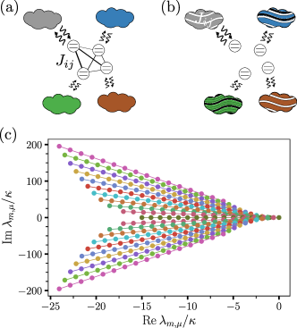
Fig. 1: (a) Schematic of the second model analyzed in this work: $N$ two-level systems interact via arbitrary Ising interactions $J_{ij}$, and are also subject to local dissipation, c.f. Eq. (12). (b) Using weak symmetry, one can make an exact mean-field decoupling for each symmetry-constrained dynamical sector, leaving one with an easily-solved but unusual independent, dissipative spin problem. (c) A similar solution method can be used for an incoherently-driven non-linear bosonic mode (c.f. Eq. (1)), enabling an exact calculation of the Liouvillian eigenvalues $\lambda_{m,\mu}$. We plot these here for $|m|\leq 10$ and $\mu\leq 15$. Each color corresponds to a different value of $|m|$. By fixing $|m|$, the level spacing $\lambda_{m,\mu+1}-\lambda_{m,\mu}=-\tilde{\kappa}_{m}-i\tilde{U}_{m}$ is constant, reflecting the non-interacting nature of the problem in each symmetry-constrained block. We work in a rotating frame where $\omega_{0}$ is shifted to $0$, and set $U=\kappa,\bar{n}_{\rm th}=0.1$.

In this Letter, we show that in many cases, the existence of a continuous weak symmetry is in fact a far more powerful tool that one might initially suspect. We show how weak symmetry can be exploited to fully and analytically diagonalize a set of non-trivial Lindblad superoperators that describe interacting, dissipative quantum systems. As explained below, this is possible because the weak symmetry makes an unusual kind of mean-field decoupling exact in each symmetry-constrained block, reducing it to an effective (but unusual) non-interacting problem (see Fig. 1). Alternatively, the solution method can be viewed as a kind of quantum-to-classical mapping. The underlying mechanism arises in a wide class of models, but for concreteness, we analyze in detail both a bosonic example (a nonlinear bosonic mode subject to thermal dissipation), and a dissipative spin model (a quantum Ising model subject to single-spin dephasing and relaxation). Both these examples are directly relevant to a variety of systems under active experimental study. Our approach yields closed form expressions for all eigenvalues and eigenvectors of the Liouvillian, enabling one to clearly identify structures that would not be apparent otherwise. This diagonalization provides a full picture of the dissipative dynamics, and also allows the calculation of a variety of observable quantities (e.g. correlation functions).

We stress that our general method is distinct from approaches used in previous work to obtain exact descriptions of specific quantum dissipative models, e.g. [9, 10, 11, 12, 13, 14, 15, 16, 17, 18, 19, 20, 21, 22, 23, 24]. Our method provides the exact dissipative spectrum and eigenvectors, and moreover, presents them in a simple and intuitive form which is tailor-made to perform analytic computations. This is crucial, as it provides the necessary starting point if one wants to make use of the burgeoning tool of Lindblad perturbation theory [25, 26, 27, 28] to more complicated systems.

Dissipative Kerr Oscillator.— Consider a bosonic mode with a Kerr (or Hubbard) type nonlinearity, subject to Markovian thermal dissipation. The evolution of the system density matrix $\hat{\rho}$ is (setting $\hbar=1$):

$$\partial_{t}\hat{\rho} =-i[\omega_{0}\hat{a}^{\dagger}\hat{a}+\frac{U}{2}\hat{a}^{\dagger}\hat{a}^{\dagger}\hat{a}\hat{a},\hat{\rho}]+\kappa(\bar{n}_{\rm th}+1)\mathcal{D}[\hat{a}]\hat{\rho}$$

$$+\kappa\bar{n}_{\rm th}\mathcal{D}[\hat{a}^{\dagger}]\hat{\rho}\equiv\mathcal{L}\hat{\rho}.$$ (1)

Here $\hat{a}$ is the mode annihilation operator, $\omega_{0}$ ($U$) is the mode natural frequency (nonlinearity), $\kappa$ the energy decay rate, and $\bar{n}_{\rm th}$ the bath’s thermal occupation. We define $\mathcal{D}[\hat{X}]\hat{\rho}\equiv\hat{X}\hat{\rho}\hat{X}^{\dagger}-\{\hat{X}^{\dagger}\hat{X},\hat{\rho}\}/2$. Eq. (1) has an obvious weak $U(1)$ symmetry, as it is invariant under $\hat{a}\to e^{-i\theta}\hat{a}$. This gives $\mathcal{L}$ a block-diagonal structure [4, 2, 3, 8, 29], which has been used previously to simplify numerical calculations [7, 8]. We show below that something more powerful is possible: despite the nonlinearity, the weak symmetry can also be used to analytically diagonalize each block and thus all of $\mathcal{L}$. Our analysis complements and extends previous studies that derive exact results for this model without explicit use of weak symmetry [12, 11, 13, 14]. In particular, our approach provides simple analytic expressions for all eigenvalues and eigenvectors of $\mathcal{L}$.

To diagonalize $\mathcal{L}$, we use the formalism of third-quantization [30, 31, 32]; relevant details can be found in the SM [33]. One first introduces four new superoperators $\bm{\hat{a}}_{\rm L}\ket{\hat{\rho}}\equiv\ket{\hat{a}\hat{\rho}}$, $\bm{\hat{a}}_{\rm R}\ket{\hat{\rho}}\equiv|\hat{\rho}\hat{a}\rangle$, $\bm{\hat{a}}_{\rm L}^{\dagger}\ket{\hat{\rho}}\equiv|\hat{a}^{\dagger}\hat{\rho}\rangle$, and $\bm{\hat{a}}_{\rm R}^{\dagger}\ket{\hat{\rho}}\equiv|\hat{\rho}\hat{a}^{\dagger}\rangle$ which we will refer to as annihilation and creation superoperators. We will also reserve the bold typeface to indicate a third-quantized superoperator $\mathcal{L}\to\mathbfcal{\hat{L}}$. We can now express our Liouvillian as $\mathbfcal{\hat{L}}=(i\omega_{0}+\kappa/2)\bm{\hat{1}}+\mathbfcal{\hat{L}}_{0}+\mathbfcal{\hat{L}}_{\rm int}$ where

$$\mathbfcal{\hat{L}}_{0} =\underline{\bm{\hat{a}}}^{\dagger}\begin{pmatrix}-i\omega_{0}-\frac{\kappa}{2}(2\bar{n}_{\rm th}+1)&\kappa\bar{n}_{\rm th}\\ \kappa(\bar{n}_{\rm th}+1)&i\omega_{0}-\frac{\kappa}{2}(2\bar{n}_{\rm th}+1)\end{pmatrix}\underline{\bm{\hat{a}}}$$ (2)

$$\mathbfcal{\hat{L}}_{\rm int} =-i\frac{U}{2}\left(\bm{\hat{a}}_{\rm L}^{\dagger}\bm{\hat{a}}_{\rm L}-\bm{\hat{a}}_{\rm R}\bm{\hat{a}}_{\rm R}^{\dagger}\right)\left(\bm{\hat{a}}_{\rm L}^{\dagger}\bm{\hat{a}}_{\rm L}+\bm{\hat{a}}_{\rm R}\bm{\hat{a}}_{\rm R}^{\dagger}-\bm{\hat{1}}\right)$$ (3)

correspond to the quadratic and interacting parts of the Linbladian respectively. Here $\underline{\bm{\hat{a}}}^{\dagger}=\begin{pmatrix}\bm{\hat{a}}_{\rm L}^{\dagger}&\bm{\hat{a}}_{\rm R}^{\dagger}\end{pmatrix}$. The quadratic part of the superoperator $\mathbfcal{\hat{L}}_{0}$ is easily diagonalized via standard third-quantization techniques [30, 31]. The nonlinear quartic terms however represent a true interaction of third-quantized bosons, and at first glance destroy exact solvability.

We now exploit the weak symmetry of our system. At the superoperator level, the weak symmetry corresponds to the invariance of Eq. (3) under $\bm{\hat{a}}_{\rm L/R}\to\bm{\hat{a}}_{\rm L/R}e^{-i\theta}$. The superoperator generating this effective unitary transformation is $\bm{\hat{a}}_{\rm L}^{\dagger}\bm{\hat{a}}_{\rm L}-\bm{\hat{a}}_{\rm R}\bm{\hat{a}}_{\rm R}^{\dagger}$, which immediately implies $[\mathbfcal{\hat{L}},\bm{\hat{a}}_{\rm L}^{\dagger}\bm{\hat{a}}_{\rm L}-\bm{\hat{a}}_{\rm R}\bm{\hat{a}}_{\rm R}^{\dagger}]=0$. Standard linear algebra then dictates that $\mathbfcal{\hat{L}}$ is block-diagonal in the eigenbasis of $\bm{\hat{a}}_{\rm L}^{\dagger}\bm{\hat{a}}_{\rm L}-\bm{\hat{a}}_{\rm R}\bm{\hat{a}}_{\rm R}^{\dagger}$. We can thus write $\mathbfcal{\hat{L}}=\bigoplus_{m}\mathbfcal{\hat{L}}_{m}$, where each block $\mathbfcal{\hat{L}}_{m}$ is indexed by $m$, an eigenvalue of $\bm{\hat{m}}\equiv\bm{\hat{a}}_{\rm L}^{\dagger}\bm{\hat{a}}_{\rm L}-\bm{\hat{a}}_{\rm R}\bm{\hat{a}}_{\rm R}^{\dagger}$. A simple calculation reveals that any outer-product of Fock states $\ket{p}\bra{q}$ is an eigenvector of the generator $\bm{\hat{m}}\ket{p}\bra{q}=[\hat{a}^{\dagger}\hat{a},\ket{p}\bra{q}]=m\ket{p}\bra{q}$ and the corresponding eigenvalue $m=p-q\in\mathbb{Z}$ characterizes the degree of coherence or off-diagonalness in Fock space. Further, since any outer product of Fock states of the form $\ket{p+n}\bra{q+n}$ has the same eigenvalue as $\ket{p}\bra{q}$, each block $\mathbfcal{\hat{L}}_{m}$ is infinite in extent.

While weak symmetry provides a block-diagonal structure, we are still left with the seemingly formidable task of diagonalizing the infinite-dimensional matrix corresponding to each block; further, apart from $m=0$, each block’s form depends on the non-trivial interaction $U$. As we now show, surprisingly these remaining tasks can be done exactly. By definition $\mathbfcal{\hat{L}}_{m}$, is the full Lindbladian projected onto the subspace spanned by eigenvectors of $\bm{\hat{m}}$ with eigenvalue $m$. We may thus, in each block $\mathbfcal{\hat{L}}_{m}$, make the substitution $\bm{\hat{m}}\to m$. Next, note that the non-linear part of $\mathcal{L}$ can be written as

$$\mathbfcal{\hat{L}}_{\rm int}=-i\frac{U}{2}\bm{\hat{m}}\times\mathbfcal{\hat{L}}_{0}^{\prime}$$ (4)

where $\mathbfcal{\hat{L}}_{0}^{\prime}=\left(\bm{\hat{a}}_{\rm L}^{\dagger}\bm{\hat{a}}_{\rm L}+\bm{\hat{a}}_{\rm R}\bm{\hat{a}}_{\rm R}^{\dagger}-\bm{\hat{1}}\right)$ is quadratic in creation an annihilation superoperators. Projecting onto the subspace indexed by $m$, when have $\mathbfcal{\hat{L}}_{\rm int}\to-iUm/2\mathbfcal{\hat{L}}_{0}^{\prime}$. We finally obtain

$$\mathbfcal{\hat{L}}_{m} =\underline{\bm{\hat{a}}}^{\dagger}\begin{pmatrix}-i\frac{Um}{2}-\frac{\kappa}{2}(2\bar{n}_{\rm th}+1)&\kappa\bar{n}_{\rm th}\\ \kappa(\bar{n}_{\rm th}+1)&-i\frac{Um}{2}-\frac{\kappa}{2}(2\bar{n}_{\rm th}+1)\end{pmatrix}\underline{\bm{\hat{a}}}$$

$$+(-i(\omega_{0}-U)m+\frac{\kappa}{2})\bm{\hat{1}}.$$ (5)

We thus have a crucial first result: in each symmetry-constrained sector, $\mathbfcal{\hat{L}}$ becomes quadratic in creation and annihilation superoperators, and can thus be diagonalized exactly. It is as though a mean-field ansatz has become exact in each block (though note the mean-field decoupling is block dependent, and results in a Liouvillian that is not in Lindblad form). We stress that the mere existence of a weak symmetry was not enough for solvability, as this by itself only guarantees the existence of the block-diagonal structure. Instead, we also needed the interacting part of the Lindbladian to factor as in Eq. (4). Identifying this general structure is a main result of this work.

As it is quadratic in creation and annihilation superoperators, Eq. (5) can be diagonalized using conventional third-quantization. One ultimately needs to diagonalize a $2\times 2$ matrix in each sector to obtain both the eigenvalues and eigenvectors. We denote the Liouvillian eigenvalues $\lambda_{m,\mu}$ where $m$ labels the different symmetry-constrained blocks (i.e. the degree of off-diagonalness), and the non-negative integer $\mu$ labels eigenmodes in a given block. It roughly characterizes the average number of particles in the eigenmode. Using the above structure (see SM [33]), we find:

$$\lambda_{m,\mu} =-i\left[\omega_{0}-U+\frac{\tilde{U}_{m}}{2}(|m|+1+2\mu)\right]m$$

$$-\frac{1}{2}\Big{[}\tilde{\kappa}_{m}(|m|+1+2\mu)-\kappa\Big{]}$$ (6)

where

$$\tilde{U}_{m} =|U|\>\text{Im}\sqrt{(\frac{\kappa}{Um})^{2}-1+2i\frac{\kappa}{Um}(2\bar{n}_{\rm th}+1)}$$ (7)

$$\tilde{\kappa}_{m} =\kappa\>\text{Re}\sqrt{1-(\frac{Um}{\kappa})^{2}+2i\frac{Um}{\kappa}(2\bar{n}_{\rm th}+1)}$$ (8)

are renormalized sector-dependent non-linearities and decay rates respectively. If $\kappa\rightarrow 0$, $\tilde{U}_{m}\rightarrow U$, whereas for non-zero $\kappa$ it is temperature dependent. We also see that the effective damping rate in each sector generically depends on temperature when $U\neq 0$. In Fig. 1 we plot the spectrum for $|m|\leq 10$ and $\mu\leq 15$. Expressions for eigenvectors are provided in the SM [33].

The ability to analytically describe the eiegenvectors and eigenvalues evidently constitutes a full solution of our system: any quantity we wish to calculate or initial state we wish to time-evolve can be readily computed using the spectral decomposition of $\mathbfcal{\hat{L}}$. This spectral information in and of itself carries a wealth of physically and experimentally relevant information. We will focus on two such examples. It is for instance interesting to note that $\tilde{U}_{m}$ and $\tilde{\kappa}_{m}$ obey

$$|U|\leq|\tilde{U}_{m}|<|U|(2\bar{n}_{\rm th}+1),$$ (9)

$$\kappa\leq\tilde{\kappa}_{m}<\kappa(2\bar{n}_{\rm th}+1),$$ (10)

where the lower bound in both cases is reached if and only if $\bar{n}_{\rm th}=0$. For a fixed non-zero temperature, the dimensionless parameter $\kappa/(Um)$ determines how close one is to reaching the lower or upper bound. For strong non-linearity or large coherences $\kappa\ll Um$ we obtain $\tilde{\kappa}_{m}\lesssim\kappa(2\bar{n}_{\rm th}+1)$. As explained in Sec. I of the [33], in this limit the right and left eigenvectors are simply outer product of Fock states and the real part of $\lambda_{m,\mu}$ corresponds to the average of the Fermi’s Golden rule decay rate for the Fock states $\ket{\mu+|m|}$ and $\ket{\mu}$ [11]. We plot $\tilde{\kappa}_{m}$ as a function of $m$ for different values of $U$ in Fig. S1 of the SM [33]. In the opposite limit of strong dissipation $\kappa\gg Um$ we see that the non-linearity scales linearly with temperature $\tilde{U}_{m}\lesssim U(2\bar{n}_{\rm th}+1)$. If we were to probe a single-particle quantity like the retarded Green’s function $G^{R}(t)=-i\Theta(t)\langle[\hat{a}(t),\hat{a}^{\dagger}(0)]\rangle$, this corresponds to the Hartree-type frequency shift one would obtain via leading-order perturbation theory.

The retarded Green’s function, which controls how the average value $\langle\hat{a}(t)\rangle$ changes in response to a weak coherent drive applied at time $t=0$, can of course be computed to all orders in $U$. Since $\hat{\rho}_{\rm ss}$ is an incoherent mixture of Fock states, it is an element of the $m=0$ block. Applying $\hat{a}^{\dagger}$ to either side of the density matrix raises the coherence by one, and thus excites all $m=1$ right eigenvectors. Using the spectral decomposition of $e^{\mathbfcal{\hat{L}}t}$ we show in the SM [33] that

$$G^{R}(t)=-i\Theta(t)\sum_{\mu=0}^{\infty}e^{\lambda_{m=1,\mu}t}\Tr(\hat{a}\hat{r}_{m=1,\mu})\Tr(\hat{l}^{\dagger}_{m=1,\mu}[\hat{a}^{\dagger},\hat{\rho}_{\rm ss}])$$

$$=-i\Theta(t)\frac{e^{-i(\omega_{0}-U)t+\frac{\kappa}{2}t}}{\left(\cosh(\frac{\tilde{\kappa}_{1}+i\tilde{U}_{1}}{2}t)+R_{1}\sinh(\frac{\tilde{\kappa}_{1}+i\tilde{U}_{1}}{2}t)\right)^{2}}.$$ (11)

where $R_{1}=(\kappa+iU(2\bar{n}_{\rm th}+1))/(\tilde{\kappa}_{1}+i\tilde{U}_{1})$ in agreement with Ref. [11]. Here $\hat{r}_{m,\mu}$ and $\hat{l}_{m,\mu}$ are the right and left eigenvectors of $\mathbfcal{\hat{L}}$ with eigenvalue $\lambda_{m,\mu}$ (see SM [33]). Fourier-transforming Eq. (11) gives us the frequency-resolved Green’s function $G^{R}[\omega]$, which can easily be accesssed in several experimental platforms. In a similar manner, higher-order response functions can be directly tied to eigenvalues and eigenvectors for higher $m$ modes.

While for clarity we have focused here on a single-mode problem, a completely analogous approach allows one to analytically diagonalize a truly many-body model, where we now have a set of bosonic modes, each with Kerr nonlinearities and thermal dissipation, coupled to one another via cross-Kerr interaction of the form $U_{ab}\hat{a}^{\dagger}\hat{a}\hat{b}^{\dagger}\hat{b}$. As we show in the SM [33], our method applies directly here: in each symmetry-constrained block, the non-trivial interaction terms become effectively quadratic. We also show this setup remains solvable if we were to add dephasing to each mode (as described by the dissipators $2\kappa_{\phi,j}\mathcal{D}[\hat{a}_{j}^{\dagger}\hat{a}_{j}]\hat{\rho}$).

Dissipative Ising Model.— We next show that our symmetry-based approach can be used for a completely different kind of system, namely a dissipative Ising model of $N$ spins. The Lindblad master equation reads

$$\partial_{t}\hat{\rho} =-i[\sum_{j<k}J_{jk}\hat{\sigma}^{z}_{j}\hat{\sigma}^{z}_{k}+\sum_{j}h_{j}\hat{\sigma}^{z}_{j},\hat{\rho}]+\sum_{j}\gamma_{-,j}\mathcal{D}[\hat{\sigma}^{-}_{j}]\hat{\rho}$$

$$+\sum_{j}\gamma_{+,j}\mathcal{D}[\hat{\sigma}^{+}_{j}]\hat{\rho}+\sum_{j}\gamma_{\phi,j}\mathcal{D}[\hat{\sigma}^{z}_{j}]\hat{\rho}\equiv\mathcal{L}\hat{\rho}.$$ (12)

It describes $N$ interacting two-level systems with arbitrary Ising couplings $J_{jk}$, each with its own local magnetic field $h_{j}$. Each spin is also subject to local spin relaxation, pumping, and dephasing characterized by the rates $\gamma_{-,j}$, $\gamma_{+,j}$ and $\gamma_{\phi,j}$ respectively. Note that Ref. 34 was able to exactly calculate equal-time averages of one and two spin operators for this model, by using a stochastic unravelling of $\mathcal{L}$ and analytically performing the average over trajectories. Our alternate approach goes much further: not only does it permit a simpler method for calculating averages, it also provides a direct means for obtaining the full dissipation spectrum, multi-time correlation functions and the full many-body density matrix.

$\mathcal{L}$ is invariant under arbitrary, independent local rotations around the $z$ axis of each spin, i.e. $\hat{\sigma}_{j}^{\pm}\to e^{\pm i\theta_{j}}\hat{\sigma}_{j}^{\pm}$. There are thus $N$ weak $U(1)$ symmetries, one for each spin, generated by the superoperators $[\hat{\sigma}^{z}_{j},\cdot]/2$. Each of these generators has two non-degenerate eigenvalues $m_{j}=\pm 1$ whose eigenvectors are coherences $\ket{\uparrow_{j}}\bra{\downarrow_{j}}=\hat{\sigma}^{+}_{j}$ and $\ket{\downarrow_{j}}\bra{\uparrow_{j}}=\hat{\sigma}^{-}_{j}$. There is also a two-fold degenerate eigenvalue $m_{j}=0$ with associated population eigenvectors $\ket{\uparrow_{j}}\bra{\uparrow_{j}}$ and $\ket{\downarrow_{j}}\bra{\downarrow_{j}}$. The Lindbladian necessarily commutes with each generator and thus takes on a block diagonal form, where each block is indexed by $\vec{M}=\{m_{1},\dots,m_{N}\}$, i.e. the vector formed by the eigenvalues of the generators. Given that the $m_{j}=\pm 1$ eigenvalues are non-degenerate whereas the $m_{j}=0$ eigenvalues are two-fold degenerate, for a specific block indexed by $\vec{M}$, we can parition our spins into a a set of “frozen” spins (i.e. spins $j$ with $m_{j}=\pm 1$) and “active” spins (i.e. spins $j$ with $m_{j}=0$). Within the specific block described by a given $\vec{M}$, the populations of the active spins can fluctuate. Formally, if we let $\hat{\rho}_{\vec{M}}$ denote the density matrix projected onto the subspace indexed by $\vec{M}$, then we have

$$\hat{\rho}_{\vec{M}} =\hat{\rho}_{\rm froz}\times\hat{\rho}_{\rm act}$$

$$=\left(\prod_{j\>\rm{frozen}}\hat{\sigma}^{m_{j}}_{j}\right)\left(\sum_{\vec{s}_{\rm act}}P(\vec{s}_{\rm act})\ket{\vec{s}_{\rm act}}\bra{\vec{s}_{\rm act}}\right)$$ (13)

where $\vec{s}_{\rm act}=\{s_{j}\>|\>j\>\rm{active}\}$ and $s_{j}\in\{\uparrow_{j},\downarrow_{j}\}$. In each block $\hat{\rho}_{\vec{M}}$ factorizes as a product over coherences $\hat{\rho}_{\rm froz}$ and a classical density matrix $\hat{\rho}_{\rm act}$ described entirely by a probability distribution $P(\vec{s}_{\rm act})$ for a ensemble of two-level systems. If we let $z(\vec{M})$ denote the number of zero eigenvalues of $\vec{M}$, which is by definition the number of active spins, then the size of the Lindblad block indexed by $\vec{M}$ is $2^{z(\vec{M})}$.

Just as in the dissipative non-linear oscillator model, the existence of weak symmetry is not enough to make the system analytically solvable, as it only guarantees the block diagonal structure of Eq. (13). There are still many blocks whose dimension is exponentially large in the number of spins, encoding what would seem to be a complicated dissipative many-body problem. Instead, further simplification emerges from the form of the interaction and the fact that a mean-field decoupling becomes exact in each symmetry sector. We show in the SM [33] that, upon projecting into the subspace indexed by $\vec{M}$, this amounts to making the replacement

$$[\sum_{j<k}J_{jk}\hat{\sigma}^{z}_{j}\hat{\sigma}^{z}_{k},\hat{\rho}]\to\sum_{j}\{J_{j}^{\rm eff}(\vec{M})\hat{\sigma}^{z}_{j},\hat{\rho}_{\vec{M}}\}$$ (14)

where we have defined $J_{j}^{\rm eff}(\vec{M})=\sum_{k\neq j}J_{jk}m_{k}$. Using Eq. (14), we therefore see that within each block, mean-field theory becomes exact: the spin-spin interaction has been replaced by a (sector-dependent) static $z$ magnetic field on each spin, $J_{j}^{\rm eff}(\vec{M})$. Combined with the local nature of the dissipation, it follows that the classical probability describing the active spin factorizes $\hat{\rho}_{\rm active}=\prod_{j\>\rm active}\left(p_{\uparrow,j}\ket{\uparrow_{j}}\bra{\uparrow_{j}}+p_{\downarrow,j}\ket{\downarrow_{j}}\bra{\downarrow_{j}}\right)$ and the equations of motion for the coefficients read

$$\partial_{t}\begin{pmatrix}p_{\uparrow,j}\\ p_{\downarrow,j}\end{pmatrix}=\begin{pmatrix}-2iJ^{\rm eff}_{j}-\gamma_{-,j}&\gamma_{+,j}\\ \gamma_{-,j}&2iJ^{\rm eff}_{j}-\gamma_{+,j}\end{pmatrix}\begin{pmatrix}p_{\uparrow,j}\\ p_{\downarrow,j}\end{pmatrix}$$ (15)

where, for the sake of compactness, we have dropped the $\vec{M}$ dependence of $J_{j}^{\rm eff}$.

The above exact decoupling has thus allowed us to map a many-body quantum problem onto an effective classical model of non-interacting spins. To see this explicitly, note that Eq. (15) would correspond precisely to a classical master equation for a two-state system if not for the strange imaginary terms $\propto J_{j}^{\rm eff}$ on the diagonals. These terms also admit a simple classical interpretation. Consider the random variable $\hat{s}_{j}=\int_{0}^{t}dt^{\prime}\hat{\sigma}^{z}_{j}(t^{\prime})$, i.e. the integral of the classical telegraph fluctuations of spin $j$. We can now interpret $2J_{j}^{\rm eff}$ as a conjugate variable to this stochastic quantity (i.e. a so-called “counting field”). Viewed as a function of $2J_{j}^{\rm eff}$, the solution to Eq. (15) allows us to obtain the time-dependent moment-generating function of $\hat{s}_{j}$, i.e. $\Lambda[2J_{j}^{\rm eff}]=\int ds_{j}P(s_{j})e^{-2iJ^{\rm eff}_{j}s_{j}}$. In a concrete sense, one concludes that the frozen spins are measuring the classical fluctuations of the active spins at a rate determined by $J_{ij}$. The upshot is that our solution method can be viewed as having made a quantum-to-classical mapping in each symmetry-constrained block.

The above exact decoupling of spins in each symmetry block immediately implies that all Liouvillian eigenvalues can be written as a sum over single-spin eigenvalues $\lambda_{j}(\vec{M})$. A simple calculation yields

$$\lambda_{j}(\vec{M})=\begin{cases}\mp i2h_{j}-\Gamma_{j}-2\gamma_{\phi,j},&j\>\rm{frozen}\\ \Gamma_{j}\pm\sqrt{\Gamma_{j}^{2}-4J^{\rm eff}_{j}(J^{\rm eff}_{j}+i\eta_{j})},&j\>\rm{active}\end{cases}$$ (16)

with $\Gamma_{j}=(\gamma_{+,j}+\gamma_{-,j})/2$ and $\eta_{j}=(\gamma_{+,j}-\gamma_{-,j})/2$. Equation (16) tells us that coherences $\ket{\downarrow_{j}}\bra{\uparrow_{j}}$ and $\ket{\uparrow_{j}}\bra{\downarrow_{j}}$ behave as expected: they oscillate with a frequency controlled by the local magnetic field and decay at a rate set by the local dephasing and relaxation processes, independently of all other spins. Populations however both decay and oscillate depending on the strength of the counting field $2J^{\rm eff}$ relative to the strength of the relaxation processes. The right and left eigenvectors factorize in a similar way, and one only needs to solve a $2\times 2$ matrix eigenvalue problem to determine their form. As such, we leave those details to the SM [33].

With both the eigenvectors and eigenvalues in hand, we can again compute any physical quantity of interest for this model. In the SM [33], we provide an example of this, for the case where all spins are initially all pointing along the $x$ direction. As mentioned earlier, analogous quantities were calculated in Ref. [34] using an alternative method. Our approach greatly simplifies the calculation, and also allows insights not possible using the trajectory method of Ref. [34], as we have access to the full dissipation spectrum. For example, we find that our many-body Liouvillian can exhibit an exceptional point (EP) structure (see SM [33]), wherein the dynamics are exceptionally sensitive to small parameter changes. Such Lindblad EPs have been the subject of considerable recent interest [35, 36, 37], though there are few truly many-body examples. Our approach can also be used to analytically find the full time-evolved many-body density matrix $\hat{\rho}(t)$ for an arbitrary initial condition (which would be difficult if not impossible to do using trajectories).

Similar to our discussion of the dissipative nonlinear bosonic model earlier, we have for clarity sketched the simplest non-trivial dissipative spin model where our symmetry-based solution method holds. The effective quantum-to-classical mapping we have established is in fact valid for a large class of dissipative spin models. For example, there are still $N$ weak $U(1)$ symmetries if we add to our model correlated spin-loss or flips for an arbitrarily large number of spins such as, e.g. $\mathcal{D}[\hat{\sigma}_{j}^{-}\hat{\sigma}_{k}^{+}]$. The block-diagonal decomposition Eq. (13) thus follows, as does the mean-field replacement Eq. (14). The only difference is that classical probability distribution describing the active spins does not factorize; nevertheless the equations of motion in each block is exactly equivalent to a classical master equation of correlated spins with a counting field for each spin $J^{\rm eff}_{j}$. This suggests that our approach could be a powerful means to attack a range of dissipative spin models.

Conclusion.— Our work shows how continuous weak symmetries can enable the analytic solution of a wide class of interacting dissipative quantum models. While we analyzed to specific examples (one bosonic, the other spin-based), we stress that the method could be applied to a variety of other systems. It also provides a powerful starting point for systematic approximation methods for systems with additional terms that break the relevant weak symmetry. For example, as our approach provides simple analytic expressions for all eigenvalues and eigenvectors, it could be directly combined with Lindblad perturbation theory [25, 26, 27]. In future work, it would be interesting to reformulate the general structure we have exploited here in terms of a dissipative Keldysh action [38, 39]; this could enable an extension of our method to non-Markovian dissipative systems.

This work is supported by the Air Force Office of Scientific Research MURI program under Grant No. FA9550-19-1-0399, and by the Simons Foundation (Award No. 669487, AC).

References

- Lieu et al. [2020] S. Lieu, R. Belyansky, J. T. Young, R. Lundgren, V. V. Albert, and A. V. Gorshkov, Phys. Rev. Lett. 125, 240405 (2020).
- Albert and Jiang [2014] V. V. Albert and L. Jiang, Phys. Rev. A 89, 022118 (2014).
- Buča and Prosen [2012] B. Buča and T. Prosen, New J. Phys. 14, 073007 (2012).
- Cattaneo et al. [2020] M. Cattaneo, G. L. Giorgi, S. Maniscalco, and R. Zambrini, Phys. Rev. A 101, 042108 (2020).
- Zhang et al. [2020] Z. Zhang, J. Tindall, J. Mur-Petit, D. Jaksch, and B. Buča, J. Phys. A: Math. Theor. 53, 215304 (2020).
- Lieu et al. [2021] S. Lieu, M. McGinley, O. Shtanko, N. R. Cooper, and A. V. Gorshkov, Kramers’ degeneracy for open systems in thermal equilibrium (2021), arXiv:2105.02888 [cond-mat.mes-hall] .
- Scarlatella et al. [2019] O. Scarlatella, A. A. Clerk, and M. Schiro, New J. Phys. 21, 043040 (2019).
- Seclì et al. [2021] M. Seclì, M. Capone, and M. Schirò, New J. Phys. 23, 063056 (2021).
- Agarwal [1970] G. S. Agarwal, Phys. Rev. A 2, 2038 (1970).
- Drummond and Walls [1980] P. D. Drummond and D. F. Walls, Journal of Physics A: Mathematical and General 13, 725 (1980).
- Dykman and Krivoglaz [1984] M. I. Dykman and M. A. Krivoglaz, Soviet Physics Reviews(vol 5) , pp 265–441 (1984).
- Peinová and Luk [1990] V. Peinová, V and A. Luk, Phys. Rev. A 41, 414 (1990).
- Chaturvedi and Srinivasan [1991a] S. Chaturvedi and V. Srinivasan, J. Mod. Opt. 38, 777 (1991a).
- Chaturvedi and Srinivasan [1991b] S. Chaturvedi and V. Srinivasan, V, Phys. Rev. A 43, 4054 (1991b).
- Stannigel et al. [2012] K. Stannigel, P. Rabl, and P. Zoller, New Journal of Physics 14, 063014 (2012).
- Torres [2014] J. M. Torres, Phys. Rev. A 89, 052133 (2014).
- Medvedyeva et al. [2016] M. V. Medvedyeva, F. H. L. Essler, and T. c. v. Prosen, Phys. Rev. Lett. 117, 137202 (2016).
- Bartolo et al. [2016] N. Bartolo, F. Minganti, W. Casteels, and C. Ciuti, Phys. Rev. A 94, 033841 (2016).
- Foss-Feig et al. [2017] M. Foss-Feig, J. T. Young, V. V. Albert, A. V. Gorshkov, and M. F. Maghrebi, Phys. Rev. Lett. 119, 190402 (2017).
- Nakagawa et al. [2018] M. Nakagawa, N. Kawakami, and M. Ueda, Phys. Rev. Lett. 121, 203001 (2018).
- Roberts and Clerk [2020] D. Roberts and A. A. Clerk, Phys. Rev. X 10, 021022 (2020).
- Buča et al. [2020] B. Buča, C. Booker, M. Medenjak, and D. Jaksch, New J. Phys. 22, 123040 (2020).
- Nakagawa et al. [2021] M. Nakagawa, N. Kawakami, and M. Ueda, Phys. Rev. Lett. 126, 110404 (2021).
- Roberts et al. [2021] D. Roberts, A. Lingenfelter, and A. Clerk, PRX Quantum 2, 020336 (2021).
- Li et al. [2014] A. C. Y. Li, F. Petruccione, and J. Koch, Scientific Reports 4, 48879 (2014).
- Li et al. [2016] A. C. Y. Li, F. Petruccione, and J. Koch, Phys. Rev. X 6, 021037 (2016).
- Hanai et al. [2021] R. Hanai, A. McDonald, and A. Clerk, Intrinsic mechanisms for drive-dependent purcell decay in superconducting quantum circuits (2021), arXiv:2106.05179 [quant-ph] .
- Albert et al. [2016] V. V. Albert, B. Bradlyn, M. Fraas, and L. Jiang, Phys. Rev. X 6, 041031 (2016).
- Minganti et al. [2018] F. Minganti, A. Biella, N. Bartolo, and C. Ciuti, Phys. Rev. A 98, 042118 (2018).
- Prosen [2008] T. Prosen, New J. Phys. 10, 043026 (2008).
- Prosen and Seligman [2010] T. Prosen and T. H. Seligman, J. Phys. A: Math. Theor. 43, 392004 (2010).
- Albert [2018] V. V. Albert, Lindbladians with multiple steady states: theory and applications (2018), arXiv:1802.00010 [quant-ph] .
- [33] See the Supplemental Material for: (I) Derivation of the eigenvalues and eigenvectors of the incoherently pumped Kerr Lindbladian Eq. (1) (II) Computing the retarded Green’s function (III) Extending the method to solving a set of harmonic oscillators coupled via a cross-Kerr interaction and subject to dephasing (IV) Derivation of the eigenvectors and eigenvalues of the dissipative Ising model Eq. (12) (V) Computing the single-spin coherence function The Supplemental Material includes Refs. [25, 26, 11, 40, 34].
- Foss-Feig et al. [2013] M. Foss-Feig, K. R. A. Hazzard, J. J. Bollinger, and A. M. Rey, Phys. Rev. A 87, 042101 (2013).
- Insinga et al. [2018] A. Insinga, B. Andresen, P. Salamon, and R. Kosloff, Phys. Rev. E 97, 062153 (2018).
- Minganti et al. [2019] F. Minganti, A. Miranowicz, R. W. Chhajlany, and F. Nori, Phys. Rev. A 100, 062131 (2019).
- Arkhipov et al. [2020] I. I. Arkhipov, A. Miranowicz, F. Minganti, and F. Nori, Phys. Rev. A 102, 033715 (2020).
- Sieberer et al. [2016] L. M. Sieberer, M. Buchhold, and S. Diehl, Rep. Prog. Phys. 79, 096001 (2016).
- Kamenev [2011] A. Kamenev, Field Theory of Non-Equilibrium Systems (Cambridge University Press, 2011).
- Heiss [2012] W. D. Heiss, J. Phys. A: Math. Theor. 45, 444016 (2012).