Bounds on heat flux for Rayleigh-Bénard convection
between Navier-slip fixed-temperature boundaries

Abstract.

We study two-dimensional Rayleigh-Bénard convection with Navier-slip, fixed temperature boundary conditions and establish bounds on the Nusselt number. As the slip-length varies with Rayleigh number ${\mathsf{Ra}}$, this estimate interpolates between the Whitehead–Doering bound by ${\mathsf{Ra}}^{\frac{5}{12}}$ for free-slip conditions [13] and classical Doering–Constantin ${\mathsf{Ra}}^{\frac{1}{2}}$ bound [4].

1. Introduction

The standard Rayleigh-Bénard convection model describes the dynamics of a fluid layer confined between two rigid plates held at different uniform temperatures: the lower plate is hot and the upper plate is cool. This temperature difference triggers density variations of the fluid layers and instability ensues, leading to a convective fluid motion and, as the control parameter Rayleigh number ${\mathsf{Ra}}$ increases, eventually becomes turbulent. Rayleigh-Bénard convection is a paradigm of nonlinear dynamics, including pattern formation and fully developed turbulence and has important applications in meteorology, oceanography and industry. A principal quantity of interest due to its relevance in geophysical and industrial applications is the vertical heat transport across the domain. This is usually expressed through the non-dimensional Nusselt number ${\mathsf{Nu}}$, which is the ratio between the total heat flux and the flux due to thermal conduction. Famously, experiment and numerical simulation suggest a power-law scaling for the Nusselt number ${\mathsf{Nu}}$

$${\mathsf{Nu}}\sim{\mathsf{Pr}}^{\alpha}{\mathsf{Ra}}^{\beta}\,\quad\mbox{ for some }\alpha,\beta\in{\mathbb{R}}\,,$$

where ${\mathsf{Ra}}$ and ${\mathsf{Pr}}$ are the non-dimensional Rayleigh and Prandtl number, respectively. In [15] a systematic theory for the scaling of the Nusselt number ${\mathsf{Nu}}$ is proposed, based on the decomposition of the global thermal and kinetic energy dissipation rates into their boundary layer and bulk contributions. As such, it is of interest to provide mathematical constraints on allowed exponents from the equations of motion.

In physical theories, scaling laws are based, in part, on the structure of (thermal and viscous) boundary layers. It is therefore interesting to understand how the heat transport properties change with respect to different choice of boundary conditions for the velocity. Most research has focused on the cases where the velocity field satisfies the no-slip [2, 3, 4, 10] and free-slip boundary conditions [11, 12, 13, 14]. In this paper we consider the nondimensional Rayleigh-Bénard convection model subject to Navier-slip boundary conditions. We note that, in contrast to the free-slip boundary conditions studied by Whitehead–Doering, the Navier-slip boundary conditions allow for vorticity to be produced at the boundary. In a sense, these conditions interpolate between the no-slip and free-slip conditions as the slip length is increased from $0$ to $\infty$. As such our bounds degenerate to those available for no-slip in the small slip length regime. As we show later in this paper, the bound ${\mathsf{Nu}}\lesssim{\mathsf{Ra}}^{\frac{1}{2}}$, holds uniformly in Prandtl number in any dimension and for any boundary conditions such that the vertical component of the velocity is zero at the (upper and lower) boundaries. At fixed $\Pr$, this bound corresponds to the classical Spiegel–Kraichnan scaling and has since been termed the “ultimate regime”. To this day, there is active debate regarding the validity of the ultimate regime insofar as it can be inferred from data [7, 5, 18]. We remark that the bound holds in any dimension and for any of the three type of boundary conditions mentioned above and its estimation uses only non-penetration of the velocity at the walls.

We now describe our setup precisely. Let $\Omega=[0,\Gamma]\times[0,1]$ be the channel with boundaries at $\{x_{2}=0\}$ and $\{x_{2}=1\}$ and periodic in $x_{1}$. We consider the Rayleigh-Bénard system [9]

$$\frac{1}{{\mathsf{Pr}}}(\partial_{t}u+u\cdot\nabla u)+\nabla p-\Delta u ={\mathsf{Ra}}Te_{2},\qquad\text{in}\ \ \Omega\,,$$ (1)

$$\nabla\cdot u =0,\qquad\quad\quad\ \text{in}\ \ \Omega,$$ (2)

$$\partial_{t}T+u\cdot\nabla T =\Delta T,\qquad\quad\ \text{in}\ \ \Omega,$$ (3)

$$\partial_{2}u_{1} =\frac{1}{{\mathsf{L}_{\mathsf{s}}}}u_{1},\qquad\ \ \text{on}\ \ \{x_{2}=0\},$$ (4)

$$-\partial_{2}u_{1} =\frac{1}{{\mathsf{L}_{\mathsf{s}}}}u_{1},\qquad\ \ \text{on}\ \ \{x_{2}=1\},$$ (5)

$$u_{2} =0,\qquad\ \quad\ \ \ \text{on}\ \ \{x_{2}=0\}\cup\{x_{2}=1\},$$ (6)

$$T =1,\qquad\quad\ \ \ \ \text{on}\ \ \{x_{2}=0\},$$ (7)

$$T =0,\qquad\quad\ \ \ \ \text{on}\ \ \{x_{2}=1\}.$$ (8)

In the horizontal direction $x_{1}$, all the unknowns are $\Gamma$-periodic. See Figure 1 for a depiction of the setup in 2d. For higher dimensions, $e_{2}$ in equation (1) becomes $e_{d}$ and the boundary conditions are (5)–(6) in all tangential components. There are two nondimensional parameters appearing in the system: the Rayleigh number ${\mathsf{Ra}}$ which expresses the strength of the thermal forcing and the Prandtl number ${\mathsf{Pr}}$ which represents the ratio of kinematic viscosity to thermal diffusivity.

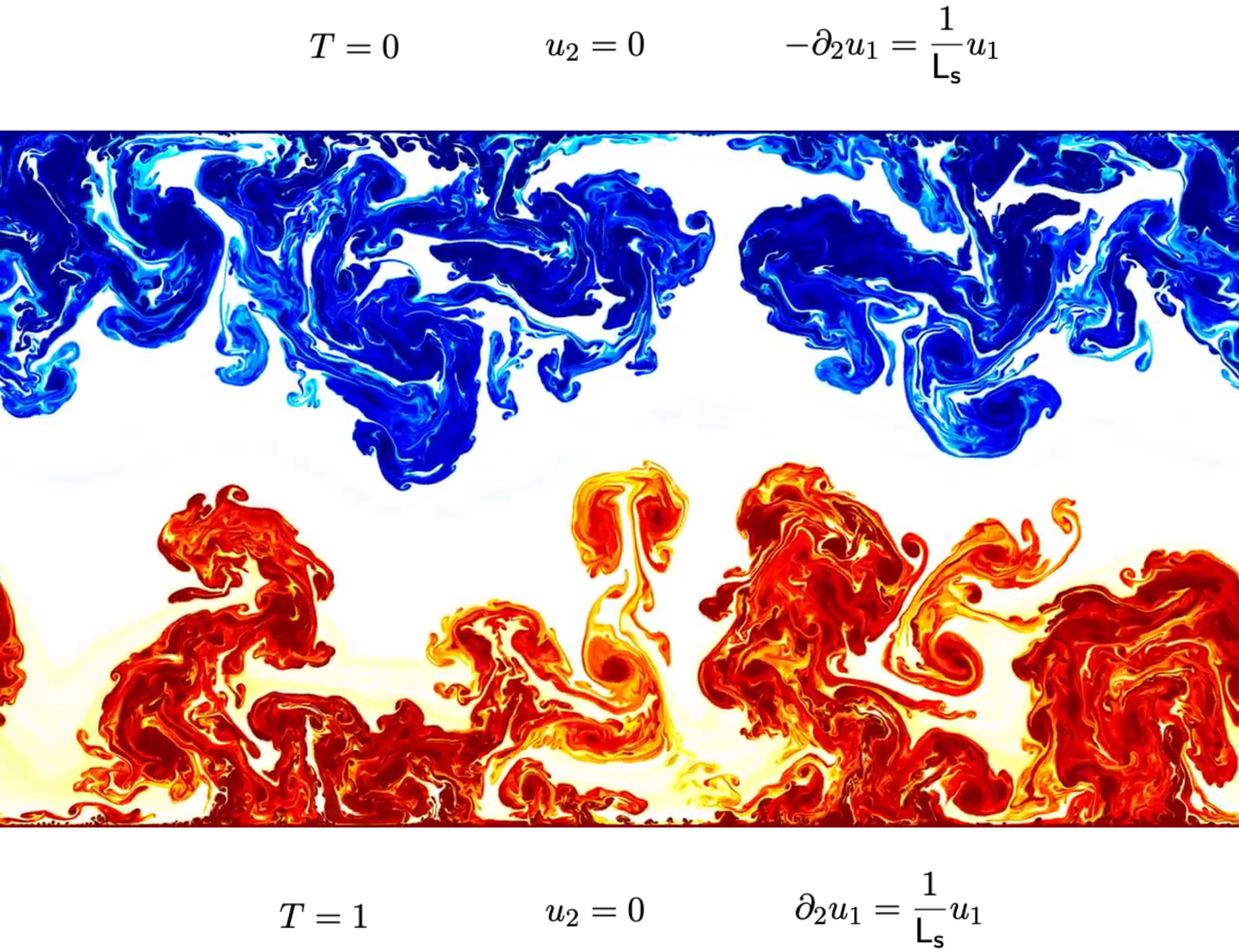
Figure 1. Visualization (with data from no-slip convection [17]) of temperature field.

As (1)–(8) is already non-dimensional, the Nusselt number is defined simply by

$${\mathsf{Nu}}:=\langle u_{2}T-\partial_{2}T\rangle,$$ (9)

where we have introduced notation for the long-time, global-in-space average

$$\langle\varphi\rangle=\limsup_{T\rightarrow\infty}\frac{1}{T}\int_{0}^{T}\frac{1}{\Gamma}\int_{0}^{\Gamma}\int_{0}^{1}\varphi(x_{1},x_{2},t)\,{\rm d}x_{2}\,{\rm d}x_{1}\,{\rm d}t.$$ (10)

We shall also write $\langle\varphi\rangle_{x_{j}}$ for the long-time and $x_{j}$ average. Our main result is the following:

Theorem 1.

Let ${\mathsf{L}_{\mathsf{s}}}>0$. Then

• For any $d\geq 2$, we have

  $${\mathsf{Nu}}\lesssim{\mathsf{Ra}}^{\frac{1}{2}}.$$ (11)

• For $d=2$, if $\Pr$ satisfies ${\mathsf{L}_{\mathsf{s}}}^{2}{\mathsf{Pr}}^{2}\geq{\mathsf{Ra}}^{\frac{3}{2}}$, then for all ${\mathsf{Ra}}>1$ it holds

  $${\mathsf{Nu}}\lesssim{\mathsf{Ra}}^{\frac{5}{12}}+{\mathsf{L}_{\mathsf{s}}}^{-2}{\mathsf{Ra}}^{\frac{1}{2}}.$$ (12)

The implicit constants depend only on $\Gamma$, $\|T_{0}\|_{L^{\infty}}$ and $\|u_{0}\|_{W^{1,r}}$ for any fixed $r\in(2,\infty)$.

Note that when ${\mathsf{L}_{\mathsf{s}}}={c_{\mathsf{s}}}{\mathsf{Ra}}^{\alpha}$ with ${c_{\mathsf{s}}}>0$ then for ${\mathsf{Pr}}\geq{c_{\mathsf{s}}}^{-1}{\mathsf{Ra}}^{\frac{3}{4}-\alpha}$ the bound (12) reads

$${\mathsf{Nu}}\lesssim{\mathsf{Ra}}^{p(\alpha)},\qquad p(\alpha):=\begin{cases}\frac{5}{12}&\text{if }\alpha\geq\frac{1}{24}\\ \frac{1}{2}-2\alpha&\text{if }0\leq\alpha\leq\frac{1}{24}\end{cases}.$$ (13)

Theorem 1 recovers the Whitehead–Doering bound of [13] in 2d with ${\mathsf{L}_{\mathsf{s}}}=\infty$ and of [14] in 3d with ${\mathsf{L}_{\mathsf{s}}}={\mathsf{Pr}}=\infty$. For smaller slip-lengths, the bound (13) approaches the classical result of Doering–Constantin [4]. Our result improves upon available bounds at fixed Prandtl numbers when the system is equipped with no-slip boundary conditions instead of (4)–(5) provided that the slip-length is sufficiently large ${\mathsf{L}_{\mathsf{s}}}\geq{c_{\mathsf{s}}}{\mathsf{Ra}}^{\frac{3}{4}}$, suggesting that the Navier-slip conditions may slightly inhibit turbulent heat transport. We remark that the work of Choffrut-Nobili-Otto [2] for no-slip boundaries (in arbitrary dimensions) gives ${\mathsf{Nu}}\lesssim{\mathsf{Ra}}^{\frac{1}{3}}$ for $\Pr\gtrsim{\mathsf{Ra}}^{\frac{1}{3}}$, which improves the bound over Doering–Constantin in that regime. Similar arguments may improve our estimates in that case. Moreover we observe that for the 3d model with free-slip boundary conditions, Wang and Whitehead proved the estimate ${\mathsf{Nu}}\lesssim{\mathsf{Ra}}^{\frac{5}{12}}+\rm{Gr^{2}}{\mathsf{Ra}}^{\frac{1}{4}}$ where the Grashof number $\rm{Gr}=\frac{{\mathsf{Ra}}}{\Pr}$ is small.

Remark 1 (Infinite Prandtl number).

For $d\geq 2$, ${\mathsf{Pr}}=\infty$, J. Whitehead (unpublished) proved ${\mathsf{Nu}}\lesssim{\mathsf{Ra}}^{\frac{5}{12}}$ for all ${\mathsf{L}_{\mathsf{s}}}>0$. In Remark 3, we show how this follows from our argument.

Inspired by [13], we employ the background field method with the simple ansatz of a background profile $\tau(x_{2})$ being constant in the bulk and linear in the boundary layers of size $\delta$. Since the Navier-slip conditions allow vorticity production at the walls, our argument is delicate in a number of places compared to that for free-slip conditions. A consequence of the vorticity production at the walls is the lack of conservation of the mean of $u_{1}$. As a result, our uniform-in-time bound for the kinetic energy grows linearly with the slip-length ${\mathsf{L}_{\mathsf{s}}}$ (see Lemma 1 and Remark 2). Another consequence is that the uniform-in-time bound for the enstrophy does not follow directly from an energy estimate for the vorticity equation. Here, following an idea in [8], we establish the uniform $L^{p}$ bounds

$$\|\omega(t)\|_{L^{p}}\leq C\Big{(}\|\omega_{0}\|_{L^{p}}+\frac{1}{{\mathsf{L}_{\mathsf{s}}}}\|u_{0}\|_{L^{2}}+{\mathsf{Ra}}\Big{)}\qquad\forall t>0,~{}p\in[1,\infty).$$ (14)

Firstly, (14) yields the long-time average enstrophy balance (36). Secondly, (14) is carefully combined with an appropriate pressure estimate (see (24)) to handle the bad boundary term in (52) in such a way that our Nusselt bound (12) recovers the result in [13] when ${\mathsf{L}_{\mathsf{s}}}\to\infty$.

Following [13], we use the long-time average energy/enstrophy balances and reduce the proof of (12) to establishing the positivity of certain quadratic functional $\mathcal{Q}$ (see Prop. 8) when parameters are suitably chosen. By obtaining a new estimate for the term $\langle\tau^{\prime}u_{2}\theta\rangle$ generated by the background field, we bypass a Fourier argument in [13] and base the proof entirely in physical space.

2. Energy Identities and Uniform Bounds

In what follows, we always consider smooth initial data so that the system (1)-(8) has a unique global smooth solution. See e.g. [1, 6]. We will repeatedly use that $\|T(t)\|_{L^{\infty}(\Omega)}\leq\max\{1,\|T_{0}\|_{L^{\infty}(\Omega)}\}$ for all $t\geq 0$ by the maximum principle. Without loss of generality, we consider initial data $\|T_{0}\|_{L^{\infty}(\Omega)}\leq 1$ so that

$$\|T\|_{L^{\infty}(\Omega)}\leq 1.$$ (15)

Now we recall the well-known (see e.g. [4]) identification of the Nusselt number with the heating rate

Proposition 1.

The Nusselt number satisfies ${\mathsf{Nu}}=\langle|\nabla T|^{2}\rangle$.

Proof.

Multiplying the temperature equation (3) by $T$, integrating by part in space, and using the incompressibility condition (2) and the boundary conditions for $u_{2}$ and $T$, we get

$$\frac{1}{2}\frac{{\rm d}}{{\rm d}t}\|T\|_{L^{2}(\Omega)}^{2}=-\|\nabla T\|_{L^{2}(\Omega)}^{2}-\int_{0}^{\Gamma}\partial_{2}T\big{|}_{x_{2}=0}{\rm d}x_{1}.$$

Since $\|T(t)\|_{L^{2}(\Omega)}$ is uniformly bounded in $t$, averaging in time yields

$$\langle|\nabla T|^{2}\rangle=-\langle\partial_{2}T\big{|}_{x_{2}=0}\rangle_{x_{1}},$$

where $\langle\cdot\rangle_{x_{1}}$ denotes the long time and $x_{1}$ average. On the other hand, if we integrate (3) in $x_{1}$ and time average, we find $\partial_{2}\langle u_{2}T-\partial_{2}T\rangle_{x_{1}}=0$. Integrating in $x_{2}$ gives

$$\langle u_{2}T-\partial_{2}T\rangle_{x_{1}}=\langle(u_{2}T-\partial_{2}T)\big{|}_{x_{2}=0}\rangle_{x_{1}}=\langle-\partial_{2}T\big{|}_{x_{2}=0}\rangle_{x_{1}}.$$

In view of the definition (9), we deduce that ${\mathsf{Nu}}=-\langle\partial_{2}T\big{|}_{x_{2}=0}\rangle_{x_{1}}=\langle|\nabla T|^{2}\rangle$. ∎

Proposition 2 (Energy Balance).

Strong solutions of (1)–(8) satisfy the balance

$$\frac{1}{2{\mathsf{Pr}}}\frac{{\rm d}}{{\rm d}t}\|u\|_{L^{2}}^{2}+\|\nabla u\|_{L^{2}}^{2}+\frac{1}{{\mathsf{L}_{\mathsf{s}}}}\left(\|u_{1}\|_{L^{2}(\{x_{2}=1\})}^{2}+\|u_{1}\|_{L^{2}(\{x_{2}=0\})}^{2}\right)={\mathsf{Ra}}\int_{\Omega}u_{2}T{\rm d}x.$$ (16)

Proof.

Dotting equation (1) with $u$, integrating over $\Omega$ and using (2) and (6), we find

$$\frac{1}{2{\mathsf{Pr}}}\frac{{\rm d}}{{\rm d}t}\|u\|_{L^{2}}^{2}=\int_{\Omega}u\cdot\Delta u+{\mathsf{Ra}}\int_{\Omega}u_{2}T{\rm d}x.$$

Using the periodicity and (4), (5) and (6) gives

$$\int_{\Omega}u\cdot\Delta u\ {\rm d}x =-\|\nabla u\|_{L^{2}}^{2}+\int_{0}^{\Gamma}\left(u\cdot\partial_{2}u\Big{|}_{x_{2}=1}-u\cdot\partial_{2}u\Big{|}_{x_{2}=0}\right){\rm d}x_{1}$$

$$=-\|\nabla u\|_{L^{2}}^{2}+\int_{0}^{\Gamma}\left(\partial_{2}u_{1}u_{1}\Big{|}_{x_{2}=1}-\partial_{2}u_{1}u_{1}\Big{|}_{x_{2}=0}\right){\rm d}x_{1}$$

$$=-\|\nabla u\|_{L^{2}}^{2}-\frac{1}{{\mathsf{L}_{\mathsf{s}}}}\left(\|u_{1}\|_{L^{2}(\{x_{2}=1\})}^{2}+\|u_{1}\|_{L^{2}(\{x_{2}=0\})}^{2}\right).$$

∎

From the energy balance, we find that the kinetic energy is bounded for all times.

Lemma 1.

The energy of $u$ satisfies the following bound

$$\|u(t)\|_{L^{2}}\leq\|u_{0}\|_{L^{2}}e^{-t\frac{2}{3}{\mathsf{Pr}}\min\{1,\frac{1}{{\mathsf{L}_{\mathsf{s}}}}\}}+3\Gamma\max\{1,{{\mathsf{L}_{\mathsf{s}}}}\}{\mathsf{Ra}},\qquad\forall t>0.$$ (17)

Proof.

From the fundamental theorem of calculus we have

$$|u_{1}(x_{1},x_{2})|^{2}\leq 2|u_{1}(x_{1},0)|^{2}+2\left(\int_{0}^{x_{2}}|\partial_{2}u_{1}(x_{1},y)|{\rm d}y\right)^{2}\leq 2|u_{1}(x_{1},0)|^{2}+2x_{2}\int_{0}^{1}|\partial_{2}u_{1}(x_{1},y)|^{2}{\rm d}y$$

and thus upon integrating over $\Omega$, we obtain

$$\|u_{1}\|_{L^{2}(\Omega)}^{2} \leq 2\|u_{1}(\cdot,0)\|_{L^{2}(0,\Gamma)}^{2}+2\|\partial_{2}u_{1}\|_{L^{2}(\Omega)}^{2}.$$

Combing this with the Poincaré inequality $\|u_{2}\|_{L^{2}(\Omega)}\leq\|\partial_{2}u_{2}\|_{L^{2}(\Omega)}$, we obtain

$$\|u\|_{L^{2}(\Omega)}^{2}\leq 2\|u_{1}(\cdot,0)\|_{L^{2}(0,\Gamma)}^{2}+3\|\nabla u\|_{L^{2}(\Omega)}^{2}.$$

In addition, the temperature $T$ obeys the maximum principle (15); hence $\|T(t)\|_{L^{2}}\leq|\Omega|\|T(t)\|_{L^{\infty}}\leq\Gamma$. Then, Proposition 2 gives

$$\frac{1}{{\mathsf{Pr}}}\frac{{\rm d}}{{\rm d}t}\|u\|_{L^{2}}\leq 2{\mathsf{Ra}}\Gamma-\frac{2}{3}\min\{1,\tfrac{1}{{\mathsf{L}_{\mathsf{s}}}}\}\|u\|_{L^{2}}.$$ (18)

∎

Remark 2.

Consider the free-slip boundary conditions $u_{2}=0$ and $\partial_{2}u_{1}=0$ on $x_{2}=0,\,1$, which can be formally obtained by setting ${\mathsf{L}_{\mathsf{s}}}=\infty$ in (6)-(7). The (spatial) mean of $u_{1}$ is conserved upon integrating the first component of (1). Appealing to the Galilean symmetry of the system, one can assume without loss of generality that the mean of $u_{1}$ is zero for all time. Consequently, the Poincaré inequality $\|u\|_{L^{2}}\leq C\|\nabla u\|_{L^{2}}$ holds. Then, the energy balance

$$\frac{1}{2{\mathsf{Pr}}}\frac{{\rm d}}{{\rm d}t}\|u\|_{L^{2}}^{2}=-\|\nabla u\|_{L^{2}}^{2}+{\mathsf{Ra}}\int_{\Omega}u_{2}T{\rm d}x$$

yields the uniform bound $\|u(t)\|_{L^{2}}\leq e^{-\frac{t}{C}}\|u_{0}\|_{L^{2}}+C\|T_{0}\|_{L^{\infty}}{\mathsf{Ra}}$. This bound is better than (17) by the factor ${\mathsf{L}_{\mathsf{s}}}$ in front of ${\mathsf{Ra}}$. On the other hand, for the Navier-slip boundary condition, the mean of $u_{1}$ is not conserved due to the generation of vorticity at the walls.

Corollary 1 (Average Energy Balance).

The following balance holds

$$\langle|\nabla u|^{2}\rangle+\frac{1}{{\mathsf{L}_{\mathsf{s}}}}\left(\langle u_{1}^{2}\big{|}_{x_{2}=1}\rangle+\langle u_{1}^{2}\big{|}_{x_{2}=0}\rangle\right)={\mathsf{Ra}}({\mathsf{Nu}}-1).$$ (19)

Proof.

Using the boundary conditions for the temperature (7)–(8), one finds

$${\mathsf{Nu}}=1+\langle u_{2}T\rangle$$ (20)

from the definition (9). Then the claim follows upon integrating (16) in time and taking the long time limit using the uniform bound for $\|u(t)\|_{L^{2}}$ given by Lemma 1. ∎

Proposition 3 (Pressure-Poisson equation).

The pressure in (1) satisfies

$$\Delta p =-\frac{1}{{\mathsf{Pr}}}\nabla u^{T}:\nabla u+{\mathsf{Ra}}\partial_{2}T\qquad\quad\ \ \text{in}\ \ \Omega\,,$$ (21)

$$-\partial_{2}p =\frac{1}{{\mathsf{L}_{\mathsf{s}}}}\partial_{1}u_{1}-{\mathsf{Ra}}\qquad\qquad\qquad\ \ \ \ \ \ \ \text{on}\ \ \{x_{2}=0\},$$ (22)

$$\partial_{2}p =\frac{1}{{\mathsf{L}_{\mathsf{s}}}}\partial_{1}u_{1}\qquad\qquad\qquad\qquad\ \ \ \ \ \ \ \ \text{on}\ \ \{x_{2}=1\}.$$ (23)

Proof.

The equation (21) follows from taking the divergence of the momentum equation. The boundary conditions come from tracing the second component of the momentum equation along the boundaries. Specifically, one has

$$\partial_{2}p=\partial_{2}^{2}u_{2}+{\mathsf{Ra}}T=-\partial_{1}\partial_{2}u_{1}+{\mathsf{Ra}}T,$$

where $\partial_{2}u_{1}$ is given by (4) and (5). ∎

Proposition 4.

For any $r\in(2,\infty)$, there exists $C=C(r,\Gamma)$ such that

$$\|p\|_{H^{1}(\Omega)}\leq C\Big{(}\frac{1}{{\mathsf{L}_{\mathsf{s}}}}\|\partial_{1}\omega\|_{L^{2}(\Omega)}+{\mathsf{Ra}}\|T\|_{L^{2}(\Omega)}+\frac{1}{\Pr}\|\omega\|_{L^{2}(\Omega)}\|\omega\|_{L^{r}(\Omega)}\Big{)}.$$ (24)

Proof.

On one hand, using the boundary conditions (22)–(23) gives

$$\int_{\Omega}p\Delta p\ {\rm d}x =-\|p\|_{\dot{H}^{1}}^{2}+\int_{0}^{\Gamma}p\partial_{2}p|^{x_{2}=1}_{x_{2}=0}{\rm d}x_{1}$$

$$=-\|\nabla p\|_{L^{2}}^{2}+\frac{1}{{\mathsf{L}_{\mathsf{s}}}}\int_{0}^{\Gamma}\left(p\partial_{1}u_{1}|_{x_{2}=1}+p\partial_{1}u_{1}|_{x_{2}=0}\right){\rm d}x_{1}-{\mathsf{Ra}}\int_{0}^{\Gamma}p|_{x_{2}=0}{\rm d}x_{1}.$$

On the other hand, using (21), (7) and (8), we find

$$\int_{\Omega}p\Delta p\ {\rm d}x =-\frac{1}{\Pr}\int_{\Omega}p\nabla u^{T}:\nabla u\ {\rm d}x-{\mathsf{Ra}}\int_{\Omega}\partial_{2}pT{\rm d}x-{\mathsf{Ra}}\int_{0}^{\Gamma}p|_{x_{2}=0}{\rm d}x_{1}.$$

Consequently,

$$\|\nabla p\|_{L^{2}}^{2} =\frac{1}{{\mathsf{L}_{\mathsf{s}}}}\int_{0}^{\Gamma}\left(p\partial_{1}u_{1}|_{x_{2}=1}+p\partial_{1}u_{1}|_{x_{2}=0}\right){\rm d}x_{1}+\frac{1}{\Pr}\int_{\Omega}p\nabla u^{T}:\nabla u\ {\rm d}x+{\mathsf{Ra}}\int_{\Omega}\partial_{2}pT{\rm d}x.$$

By virtue of the Sobolev trace inequality and Hölder’s inequality, it follows that

$$\|\nabla p\|_{L^{2}}^{2} \lesssim\frac{1}{{\mathsf{L}_{\mathsf{s}}}}\|p\|_{{H}^{1}}\|\partial_{1}u_{1}\|_{{H}^{1}}+{\mathsf{Ra}}\|p\|_{{H}^{1}}\|T\|_{L^{2}}+\frac{1}{\Pr}\|p\nabla u^{T}:\nabla u\|_{L^{1}}.$$

For any $r\in(2,\infty)$, letting $\frac{1}{q}=\frac{1}{2}-\frac{1}{r}$, we have $q\in(2,\infty)$ and

$$\|p\nabla u^{T}:\nabla u\|_{L^{1}}\leq\|p\|_{L^{q}}\|\nabla u\|_{L^{2}}\|\nabla u\|_{L^{r}}\leq C\|p\|_{H^{1}}\|\omega\|_{L^{2}}\|\omega\|_{L^{r}},$$

where we use the Sobolev embedding and (62).

Since $p$ has mean zero, we have $\|p\|_{H^{1}}\leq C\|\nabla p\|_{L^{2}}$, so that upon using $\partial_{1}u_{1}=-\partial_{2}u_{2}$ we get

$$\|p\|_{H^{1}} \lesssim\frac{1}{{\mathsf{L}_{\mathsf{s}}}}\|\partial_{2}u_{2}\|_{{H}^{1}}+{\mathsf{Ra}}\|T\|_{L^{2}}+\frac{C}{\Pr}\|\omega\|_{L^{2}}\|\omega\|_{L^{r}}.$$

From Lemma 6 and (62), $\|\nabla u\|_{L^{2}}=\|\omega\|_{L^{2}}$ and $\|\partial_{2}u_{2}\|_{{H}^{1}}\leq C\|\partial_{1}\omega\|_{L^{2}}$, whence (24) follows. ∎

Proposition 5 (Vorticity formulation).

The vorticity $\omega=\nabla^{\perp}\cdot u$ where $\nabla^{\perp}=(-\partial_{2},\partial_{1})$ satisfies

$$\frac{1}{{\mathsf{Pr}}}(\partial_{t}\omega+u\cdot\nabla\omega)-\Delta\omega ={\mathsf{Ra}}\partial_{1}T\qquad\text{in}\ \ \Omega\,,$$ (25)

$$-\omega =\frac{1}{{\mathsf{L}_{\mathsf{s}}}}u_{1}\qquad\ \ \text{on}\ \ \{x_{2}=0\},$$ (26)

$$\omega =\frac{1}{{\mathsf{L}_{\mathsf{s}}}}u_{1}\qquad\ \ \text{on}\ \ \{x_{2}=1\}.$$ (27)

Proof.

Equation (25) follows from taking the curl of the momentum equation (1). The boundary conditions (26)–(27) follow from the conditions (4)–(5) since the vorticity on the boundary is simply $\omega=-\partial_{2}u_{1}$ upon recalling (6). ∎

Lemma 2.

The normal derivative of vorticity satisfies

$$-\partial_{2}\omega=\frac{1}{{\mathsf{Pr}}}\big{(}\partial_{t}u_{1}+u_{1}\partial_{1}u_{1}\big{)}+\partial_{1}p,\quad\text{on}\quad\{x_{2}=0\}\ \text{and}\ \{x_{2}=1\}.$$ (28)

Proof.

Using incompressibility of $u$, we find

$$\partial_{2}\omega =-\partial_{2}^{2}u_{1}+\partial_{1}\partial_{2}u_{2}=-\Delta u_{1}.$$ (29)

From the first component of (1) traced on the boundary (using $u_{2}=0$ there) we have

$$\Delta u_{1}=\frac{1}{{\mathsf{Pr}}}\big{(}\partial_{t}u_{1}+u_{1}\partial_{1}u_{1}\big{)}+\partial_{1}p.$$ (30)

∎

Proposition 6 (Enstrophy Balance).

The following identity holds

$$\frac{1}{2{\mathsf{Pr}}}\frac{{\rm d}}{{\rm d}t}\|\omega\|_{L^{2}}^{2} +\frac{1}{2{\mathsf{L}_{\mathsf{s}}}{\mathsf{Pr}}}\frac{{\rm d}}{{\rm d}t}\left(\|u_{1}\|_{L^{2}(\{x_{2}=1\})}^{2}+\|u_{1}\|_{L^{2}(\{x_{2}=0\})}^{2}\right)+\|\nabla\omega\|_{L^{2}}^{2}$$ (31)

$$=\frac{1}{{\mathsf{L}_{\mathsf{s}}}}\left(\int_{0}^{\Gamma}p\partial_{1}u_{1}\Big{|}_{x_{2}=1}{\rm d}x_{1}+\int_{0}^{\Gamma}p\partial_{1}u_{1}\Big{|}_{x_{2}=0}{\rm d}x_{1}\right)+{\mathsf{Ra}}\int_{\Omega}\omega\partial_{1}T{\rm d}x.$$

Proof.

Multiplying (25) by $\omega$ and integrating over the domain, we obtain

$$\frac{1}{2{\mathsf{Pr}}}\frac{{\rm d}}{{\rm d}t}\|\omega\|_{L^{2}}^{2}=\int_{\Omega}\omega\Delta\omega{\rm d}x+{\mathsf{Ra}}\int_{\Omega}\omega\partial_{1}T{\rm d}x,$$ (32)

where we have use the non-penetration boundary conditions for the velocity (6). Now note that

$$\int_{\Omega}\omega\Delta\omega{\rm d}x =-\|\nabla\omega\|_{L^{2}}^{2}+\int_{0}^{\Gamma}\omega\partial_{2}\omega\Big{|}_{x_{2}=1}{\rm d}x_{1}-\int_{0}^{\Gamma}\omega\partial_{2}\omega\Big{|}_{x_{2}=0}{\rm d}x_{1}$$

$$=-\|\nabla\omega\|_{L^{2}}^{2}+\frac{1}{{\mathsf{L}_{\mathsf{s}}}}\int_{0}^{\Gamma}u_{1}\partial_{2}\omega\Big{|}_{x_{2}=1}{\rm d}x_{1}+\frac{1}{{\mathsf{L}_{\mathsf{s}}}}\int_{0}^{\Gamma}u_{1}\partial_{2}\omega\Big{|}_{x_{2}=0}{\rm d}x_{1}$$

$$=-\|\nabla\omega\|_{L^{2}}^{2}-\frac{1}{2{\mathsf{L}_{\mathsf{s}}}{\mathsf{Pr}}}\frac{{\rm d}}{{\rm d}t}\left(\int_{0}^{\Gamma}u_{1}^{2}\Big{|}_{x_{2}=1}{\rm d}x_{1}+\int_{0}^{\Gamma}u_{1}^{2}\Big{|}_{x_{2}=0}{\rm d}x_{1}\right)$$

$$\qquad+\frac{1}{{\mathsf{L}_{\mathsf{s}}}}\left(\int_{0}^{\Gamma}\partial_{1}u_{1}p\Big{|}_{x_{2}=1}{\rm d}x_{1}+\int_{0}^{\Gamma}\partial_{1}u_{1}p\Big{|}_{x_{2}=0}{\rm d}x_{1}\right),$$

where we have used Lemma 2 together with periodicity of the function $u_{1}$ in $x_{1}$. ∎

Next we provide uniform in time bounds for the vorticity

Lemma 3 ($L^{p}$ vorticity bounds).

Let ${\mathsf{L}_{\mathsf{s}}}\geq 1$, $p\in[1,\infty)$. There is $C=C(p,\Gamma)<\infty$ so that

$$\|\omega(t)\|_{L^{p}}\leq C\Big{(}\|\omega_{0}\|_{L^{p}}+\frac{1}{{\mathsf{L}_{\mathsf{s}}}}\|u_{0}\|_{L^{2}}+{\mathsf{Ra}}\Big{)}\qquad\forall t>0.$$ (33)

Proof.

Since $\Omega$ is bounded it suffices to prove (33) for $p\in(2,\infty)$. To this end, we follow a strategy used in [8]. For arbitrary $T>0$ set

$$\Lambda:=\frac{1}{{\mathsf{L}_{\mathsf{s}}}}\|u_{1}\|_{L^{\infty}(\{x_{2}=0,1\}\times(0,T))}$$

and consider the problems

$$\frac{1}{{\mathsf{Pr}}}(\partial_{t}\tilde{\omega}_{\pm}+u\cdot\nabla\tilde{\omega}_{\pm})-\Delta\tilde{\omega}_{\pm} ={\mathsf{Ra}}\partial_{1}T\qquad\text{in}\ \ \Omega\,,$$

$$\tilde{\omega}_{\pm}|_{t=0} =\pm|\omega_{0}|\qquad\ \ \text{in}\ \ \Omega,$$

$$\tilde{\omega}_{\pm} =\pm\Lambda\qquad\ \ \ \ \text{on}\ \ \{x_{2}=0\}\cup\{x_{2}=1\}.$$

Now let $\omega^{\prime}_{\pm}:=\omega-\tilde{\omega}_{\pm}$. This quantity satisfies

$$\frac{1}{{\mathsf{Pr}}}(\partial_{t}\omega^{\prime}_{\pm}+u\cdot\nabla{\omega}^{\prime}_{\pm})-\Delta\omega^{\prime}_{\pm} =0\qquad\qquad\ \ \quad\quad\ \text{in}\ \ \Omega\,,$$

$$\omega^{\prime}_{\pm}|_{t=0} =\omega_{0}\mp|\omega_{0}|\ \ \qquad\ \ \ \text{in}\ \ \Omega$$

$$-\omega^{\prime}_{\pm} =\frac{1}{{\mathsf{L}_{\mathsf{s}}}}u_{1}\pm\Lambda\qquad\ \ \ \ \text{on}\ \ \{x_{2}=0\},$$

$$\omega^{\prime}_{\pm} =\frac{1}{{\mathsf{L}_{\mathsf{s}}}}u_{1}\mp\Lambda\qquad\ \ \ \ \text{on}\ \ \{x_{2}=1\}.$$

By the maximum principle, we have $\omega^{\prime}_{+}\leq 0$ and $\omega^{\prime}_{-}\geq 0$ a.e. $\Omega\times[0,T)$. Thus we obtain $\tilde{\omega}_{-}\leq\omega\leq\tilde{\omega}_{+}$ and hence

$$|\omega|\leq\max\{|\tilde{\omega}_{+}|,|\tilde{\omega}_{-}|\}\qquad\text{a.e.}\qquad\Omega\times[0,T).$$ (34)

We now bound $\tilde{\omega}_{\pm}$ in $L^{p}$. We focus on $\tilde{\omega}=\tilde{\omega}_{+}$, the other is similar. Let $\hat{\omega}:=\tilde{\omega}-\Lambda$. This solves

$$\frac{1}{{\mathsf{Pr}}}(\partial_{t}\hat{\omega}+u\cdot\nabla\hat{\omega})-\Delta\hat{\omega} ={\mathsf{Ra}}\partial_{1}T\qquad\quad\quad\ \text{in}\ \ \Omega\,,$$

$$\hat{\omega}|_{t=0} =|\omega_{0}|-\Lambda\ \ \qquad\ \ \text{in}\ \ \Omega,$$

$$\omega =0\qquad\qquad\ \ \ \ \quad\text{on}\ \ \{x_{2}=0\}\cup\{x_{2}=1\}.$$

We now perform $L^{p}$ estimates; multiplying by $\hat{\omega}|\hat{\omega}|^{p-2}$ where $p>2$ we find

$$\frac{1}{p}\frac{{\rm d}}{{\rm d}t}\|\hat{\omega}\|_{L^{p}}^{p}+(p-1)\int_{\Omega}|\nabla\hat{\omega}|^{2}|\hat{\omega}|^{p-2}{\rm d}x=-{\mathsf{Ra}}\int_{\Omega}\partial_{1}(\hat{\omega}|\hat{\omega}|^{p-2})T{\rm d}x.$$

We bound using Cauchy-Schwarz and Young’s inequality

$${\mathsf{Ra}}\left|\int_{\Omega}\partial_{1}(\hat{\omega}|\hat{\omega}|^{p-2})T{\rm d}x\right| \leq(p-1)\left(\int_{\Omega}|\nabla\hat{\omega}|^{2}|\hat{\omega}|^{p-2}{\rm d}x\right)^{\frac{1}{2}}\left({\mathsf{Ra}}^{2}\int_{\Omega}|\hat{\omega}|^{p-2}T^{2}{\rm d}x\right)^{\frac{1}{2}}$$

$$\leq\frac{p-1}{2}\int_{\Omega}|\nabla\hat{\omega}|^{2}|\hat{\omega}|^{p-2}{\rm d}x+\frac{p-1}{2}|\Omega|^{\frac{2}{p}}{\mathsf{Ra}}^{2}\|\hat{\omega}\|_{L^{p}}^{p-2},$$

where we used that $\|T\|_{L^{\infty}}=1$. Thus we obtain

$$\frac{1}{p}\frac{{\rm d}}{{\rm d}t}\|\hat{\omega}\|_{L^{p}}^{p}+\frac{p-1}{2}\int_{\Omega}|\nabla\hat{\omega}|^{2}|\hat{\omega}|^{p-2}{\rm d}x\leq\frac{p-1}{2}|\Omega|^{\frac{2}{p}}{\mathsf{Ra}}^{2}\|\hat{\omega}\|_{L^{p}}^{p-2}.$$

Finally, since $\hat{\omega}$ vanishes on the boundary, we have the Poincaré inequality

$$\int_{\Omega}|\nabla\hat{\omega}|^{2}|\hat{\omega}|^{p-2}{\rm d}x=\frac{4}{p^{2}}\|\nabla|\omega|^{\frac{p}{2}}\|_{L^{2}}^{2}\geq\frac{4}{p^{2}C_{p}^{2}}\||\omega|^{\frac{p}{2}}\|_{L^{2}}^{2}=\frac{4}{p^{2}C_{p}^{2}}\|\omega\|_{L^{p}}^{p}$$

Thus we obtain (dividing through by $\|\hat{\omega}\|_{L^{p}}^{p-2}$) the inequality

$$\frac{{\rm d}}{{\rm d}t}\|\hat{\omega}\|_{L^{p}}^{2}\leq-\frac{p-1}{2}\frac{4}{p^{2}C_{p}^{2}}\|\hat{\omega}\|_{L^{p}}^{2}+\ \frac{p-1}{2}|\Omega|^{\frac{2}{p}}{\mathsf{Ra}}^{2}.$$

It follows that for all $t\geq 0$

$$\|\hat{\omega}(t)\|_{L^{p}}\leq\|\hat{\omega}_{0}\|_{L^{p}}e^{-t\frac{(p-1)}{p^{2}C_{p}^{2}}}+\frac{pC_{p}}{2}|\Omega|^{\frac{1}{p}}{\mathsf{Ra}}\leq C\Big{(}\|\omega_{0}\|_{L^{p}}e^{-\frac{t}{C}}+\Lambda+{\mathsf{Ra}}\Big{)},\quad C=C(p,\Gamma).$$ (35)

Given this bound, we estimate $\Lambda$ using interpolation as follows

$$\Lambda\leq\frac{1}{{\mathsf{L}_{\mathsf{s}}}}\|u\|_{L^{\infty}(\Omega\times(0,T))} \leq\frac{C}{{\mathsf{L}_{\mathsf{s}}}}\|u\|_{L^{\infty}([0,T];L^{2}_{x})}^{\theta}\|\nabla u\|_{L^{\infty}([0,T];L^{p}_{x})}^{1-\theta}+\frac{C}{{\mathsf{L}_{\mathsf{s}}}}\|u\|_{L^{\infty}([0,T];L^{2}_{x})}$$

$$\leq\frac{C}{{\mathsf{L}_{\mathsf{s}}}}\|u\|_{L^{\infty}([0,T];L^{2}_{x})}^{\theta}\|\omega\|_{L^{\infty}([0,T];L^{p}_{x})}^{1-\theta}+\frac{C}{{\mathsf{L}_{\mathsf{s}}}}\|u\|_{L^{\infty}([0,T];L^{2}_{x})}$$

$$\leq C_{\varepsilon}\left(\frac{1}{{\mathsf{L}_{\mathsf{s}}}^{\frac{1}{\theta}}}+\frac{1}{{\mathsf{L}_{\mathsf{s}}}}\right)\|u\|_{L^{\infty}([0,T];L^{2}_{x})}+{\varepsilon}\|\omega\|_{L^{\infty}([0,T];L^{p}_{x})},$$

where $\theta=\frac{p-2}{2p-2}\in(0,1)$, ${\varepsilon}>0$ is arbitrary and, appealing to Lemma 7, we used $\|\nabla u\|_{L^{p}}\lesssim\|\omega\|_{L^{p}}$. By virtue of Lemma 1, for ${\mathsf{L}_{\mathsf{s}}}\geq 1$ we obtain

$$\Lambda\leq C_{\varepsilon}\left(\frac{1}{{\mathsf{L}_{\mathsf{s}}}}\|u_{0}\|_{L^{2}}+{\mathsf{Ra}}\right)+{\varepsilon}\|\omega\|_{L^{\infty}([0,T];L^{p}_{x})}.$$

In view of this, (34) and (35), choosing $\varepsilon$ small enough gives

$$\|\omega\|_{L^{\infty}([0,T];L^{p})}\leq C\Big{(}\|\omega_{0}\|_{L^{p}}+\frac{1}{{\mathsf{L}_{\mathsf{s}}}}\|u_{0}\|_{L^{2}}+{\mathsf{Ra}}\Big{)},$$

where $C$ is independent of $T$. Since $T>0$ is arbitrary, this completes the proof. ∎

An immediate consequence of the enstrophy balance (31) and the uniform vorticity bound (33) is the following global balance

Corollary 2 (Average Enstrophy Balance).

We have the balance for long-time averages

$$\langle|\nabla\omega|^{2}\rangle=\frac{1}{{\mathsf{L}_{\mathsf{s}}}}\left(\langle p\partial_{1}u_{1}\big{|}_{x_{2}=1}\rangle+\langle p\partial_{1}u_{1}\big{|}_{x_{2}=0}\rangle\right)+{\mathsf{Ra}}\langle\omega\partial_{1}T\rangle.$$ (36)

3. Proof of Theorem 1

The theorem follows by an application of the background field method [4]. This method is based on adopting the ansatz

$$T(x_{1},x_{2},t)=:\tau(x_{2})+\theta(x_{1},x_{2},t).$$ (37)

We choose the “background” profile $\tau:[0,1]\to[0,1]$ to be the continuous function given by

$$\tau(z):=1-\frac{1}{2\delta}\begin{cases}z&z\in[0,\delta]\\ \delta&z\in(\delta,1-\delta)\\ z+2\delta-1&z\in[1-\delta,1]\end{cases},$$ (38)

for some $\delta>0$ to be chosen later in the proof. Note that

$$\tau^{\prime}(z)=-\frac{1}{2\delta}\begin{cases}1&z\in[0,\delta)\\ 0&z\in(\delta,1-\delta)\\ 1&z\in(1-\delta,1]\end{cases}.$$ (39)

Note that $\|\tau^{\prime}\|_{L^{2}([0,1])}^{2}=\frac{1}{2\delta}$. Note that $\theta$ vanishes at the boundaries $x_{2}=\{0,1\}$.

Proposition 7.

With $\theta$ and $\tau$ defined by (37) and (38), the following identity holds

$${\mathsf{Nu}}-\frac{1}{2\delta}=-\langle|\nabla\theta|^{2}\rangle-2\langle\tau^{\prime}u_{2}\theta\rangle.$$ (40)

Proof.

According to Proposition 1, the decomposition (37) and the profile (39), we have

$${\mathsf{Nu}} =\langle|\nabla\theta|^{2}\rangle+\|\tau^{\prime}\|_{L^{2}([0,1])}^{2}+2\langle\tau^{\prime}\partial_{2}\theta\rangle.$$ (41)

Inserting now the ansatz (37) into (3), we find the fluctuation $\theta$ satisfies

$$\partial_{t}\theta+u_{2}\tau^{\prime}+u\cdot\nabla\theta-\Delta\theta-\tau^{\prime\prime} =0\ \qquad\ \ \text{in}\ \ \Omega\,,$$ (42)

$$\theta =0\qquad\ \ \text{on}\ \ \{x_{2}=0\}\cup\{x_{2}=1\}.$$ (43)

Integrating (42) against $\theta$ and taking the long-time average (using the fact that $\theta$, like $T$, is uniformly bounded in time), we obtain

$$\langle\tau^{\prime}\partial_{2}\theta\rangle=-\langle|\nabla\theta|^{2}\rangle-\langle\tau^{\prime}u_{2}\theta\rangle.$$ (44)

This argument can be made rigorous by smooth approximation of the profile $\tau$. Inserting this equality above yields the claimed identity. ∎

Similarly to the bound of Doering–Constantin for the no-slip boundary condition [4], we have

Lemma 4.

For any ${\mathsf{L}_{\mathsf{s}}}>0$, we have ${\mathsf{Nu}}\lesssim{\mathsf{Ra}}^{\frac{1}{2}}$.

Proof.

Equation (40) implies ${\mathsf{Nu}}\leq\frac{1}{2\delta}-2\langle\tau^{\prime}u_{2}\theta\rangle$. Since $\tau^{\prime}=\frac{1}{2\delta}$ on its support $(0,\delta)\cup(1,1-\delta)$ and $\theta$ and $u_{2}$ vanish on $x_{2}=0,\ 1$, we have

$$|\theta(x_{1},x_{2})|\leq\sqrt{\delta}\|\partial_{2}\theta(x_{1},\cdot)\|_{L^{2}(0,1)}\quad\forall x_{2}\in(0,\delta)\cup(1,1-\delta)$$

and similarly for $u_{2}$. Consequently,

$$\frac{1}{\Gamma}\int_{0}^{\Gamma}\int_{0}^{1}2|\tau^{\prime}u_{2}\theta|{\rm d}x_{2}{\rm d}x_{1}\leq\delta\frac{1}{\Gamma}\|\partial_{2}u_{2}\|_{L^{2}(\Omega)}\|\partial_{2}\theta\|_{L^{2}(\Omega)}.$$

Integrating in time and applying the Cauchy-Schwarz inequality gives

$$|\langle-2\tau^{\prime}u_{2}\theta\rangle|\leq 2\delta\langle|\partial_{2}u_{2}|^{2}\rangle^{\frac{1}{2}}\langle|\partial_{2}\theta|^{2}\rangle^{\frac{1}{2}}.$$ (45)

Appealing to Proposition 1 and Corollary 1 we deduce

$${\mathsf{Nu}}\leq\frac{1}{2\delta}+2\delta({\mathsf{Nu}})^{\frac{1}{2}}(({\mathsf{Nu}}-1){\mathsf{Ra}})^{\frac{1}{2}}\lesssim\frac{1}{2\delta}+2\delta{\mathsf{Nu}}{\mathsf{Ra}}^{\frac{1}{2}}\,.$$ (46)

Choosing $\delta\sim{\mathsf{Nu}}^{-\frac{1}{2}}{\mathsf{Ra}}^{-\frac{1}{4}}\,$ by balancing the contributions of each term yields ${\mathsf{Nu}}\lesssim{\mathsf{Ra}}^{\frac{1}{2}}\,$. ∎

To improve the bound, we follow [13] by using the energy and enstrophy balances

(a) $$:=\langle|\nabla\omega|^{2}\rangle-\frac{1}{{\mathsf{L}_{\mathsf{s}}}}\left(\langle p\partial_{1}u_{1}\big{|}_{x_{2}=1}\rangle+\langle p\partial_{1}u_{1}\big{|}_{x_{2}=0}\rangle\right)-{\mathsf{Ra}}\langle\omega\partial_{1}T\rangle,$$

(b) $$:=\langle|\nabla u|^{2}\rangle+\frac{1}{{\mathsf{L}_{\mathsf{s}}}}\left(\langle u_{1}^{2}\big{|}_{x_{2}=1}\rangle+\langle u_{1}^{2}\big{|}_{x_{2}=0}\rangle\right)-{\mathsf{Ra}}({\mathsf{Nu}}-1).$$

Note that $\textbf{(a)}=\textbf{(b)}=0$ by Corollary 1 and 2. Thus in view of (40) we have

$${\mathsf{Nu}}=\frac{1}{2\delta}-\langle|\nabla\theta|^{2}\rangle-2\langle\tau^{\prime}u_{2}\theta\rangle-\frac{b}{{\mathsf{Ra}}}\textbf{(b)}-a\textbf{(a)},$$ (47)

for all $b\in[0,1)$ and $a\in\mathbb{R}$.

Proposition 8.

Let $\delta>0$, $b\in[0,1)$, $a>0$ and $M>0$. Then the following identity holds

$$(1-b){\mathsf{Nu}}+b =\frac{1}{2\delta}+M{\mathsf{Ra}}^{2}-\mathcal{Q}[\theta,u,\tau],$$ (48)

where $\mathcal{Q}[\theta,u,\tau]$ is defined by

$$\mathcal{Q}[\theta,u,\tau] :=M{\mathsf{Ra}}^{2}+\langle|\partial_{1}\theta|^{2}\rangle+\langle|\partial_{2}\theta|^{2}\rangle+2\langle\tau^{\prime}u_{2}\theta\rangle$$

$$\qquad+\frac{b}{{\mathsf{Ra}}}\langle|\omega|^{2}\rangle+\frac{b}{{\mathsf{Ra}}{\mathsf{L}_{\mathsf{s}}}}\left(\langle u_{1}^{2}\big{|}_{x_{2}=1}\rangle+\langle u_{1}^{2}\big{|}_{x_{2}=0}\rangle\right)$$

$$\qquad\quad+a\langle|\nabla\omega|^{2}\rangle-\frac{a}{{\mathsf{L}_{\mathsf{s}}}}\left(\langle p\partial_{1}u_{1}\big{|}_{x_{2}=1}\rangle+\langle p\partial_{1}u_{1}\big{|}_{x_{2}=0}\rangle\right)-a{\mathsf{Ra}}\langle\omega\partial_{1}\theta\rangle.$$ (49)

The strategy is to show that $\mathcal{Q}$ is non-negative for an appropriate choice of $\delta:=\delta({\mathsf{Ra}})$. Then (48) will yield the desired bound on the Nusselt number. This requires bounds for the pressure and for $2\langle\tau^{\prime}u_{2}\theta\rangle$, where the former is handled by virtue of (24) and the latter requires a bound different from (45). The main result is

Proposition 9.

There exists a universal constant $L_{0}>0$ such that for all ${\mathsf{L}_{\mathsf{s}}}\geq L_{0}$ and $\Pr$ such that ${\mathsf{L}_{\mathsf{s}}}^{2}{\mathsf{Pr}}^{2}\geq{\mathsf{Ra}}^{\frac{3}{2}}$, we have

$${\mathsf{Nu}}\lesssim{\mathsf{Ra}}^{\frac{5}{12}}+{\mathsf{L}_{\mathsf{s}}}^{-2}{\mathsf{Ra}}^{\frac{1}{2}},\qquad\forall\\ Ra>1.$$ (50)

Here, the implicit constant depends only on $\Gamma$, $\|T_{0}\|_{L^{\infty}}$ and $\|u_{0}\|_{W^{1,r}}$ for any fixed $r\in(2,\infty)$.

Proof.

First we use Cauchy-Schwarz and Young’s inequality to get

$$|a{\mathsf{Ra}}\langle\omega\partial_{1}\theta\rangle|\leq\frac{a^{2}{\mathsf{Ra}}^{2}}{2}\langle|\omega|^{2}\rangle+\frac{1}{2}\langle|\partial_{1}\theta|^{2}\rangle,$$ (51)

so that $\mathcal{Q}$ of Proposition 8 enjoys the lower bound

$$\mathcal{Q}[\theta,u,\tau] \geq M{\mathsf{Ra}}^{2}+\frac{1}{2}\langle|\partial_{1}\theta|^{2}\rangle+\langle|\partial_{2}\theta|^{2}\rangle+2\langle\tau^{\prime}u_{2}\theta\rangle+\left(\frac{b}{{\mathsf{Ra}}}-\frac{a^{2}{\mathsf{Ra}}^{2}}{2}\right)\langle|\omega|^{2}\rangle+a\langle|\nabla\omega|^{2}\rangle$$ (52)

$$\qquad+\frac{b}{{\mathsf{Ra}}{\mathsf{L}_{\mathsf{s}}}}\left(\langle u_{1}^{2}\big{|}_{x_{2}=1}\rangle+\langle u_{1}^{2}\big{|}_{x_{2}=0}\rangle\right)-\frac{a}{{\mathsf{L}_{\mathsf{s}}}}\left(\langle p\partial_{1}u_{1}\big{|}_{x_{2}=1}\rangle+\langle p\partial_{1}u_{1}\big{|}_{x_{2}=0}\rangle\right).$$

Note that from the Sobolev trace inequality and the incompressibility, we have

$$\frac{a}{{\mathsf{L}_{\mathsf{s}}}}\left|\langle p\partial_{1}u_{1}\big{|}_{x_{2}=1}\rangle+\langle p\partial_{1}u_{1}\big{|}_{x_{2}=0}\rangle\right|\leq\frac{C_{1}a}{{\mathsf{L}_{\mathsf{s}}}}\langle\|p\|_{H^{1}}\|\partial_{2}u_{2}\|_{L^{2}}\rangle\leq\frac{C_{1}a}{{\mathsf{L}_{\mathsf{s}}}}\langle\|\nabla p\|_{L^{2}}\|\partial_{1}\omega\|_{L^{2}}\rangle,$$

where we used (62) and $C_{1}=C_{1}(\Gamma)$. To bound the pressure, we recall from (24) that for any $r\in(2,\infty)$,

$$\|p\|_{H^{1}(\Omega)}\leq C\Big{(}\frac{1}{{\mathsf{L}_{\mathsf{s}}}}\|\partial_{1}\omega\|_{L^{2}(\Omega)}+{\mathsf{Ra}}\|T\|_{L^{2}(\Omega)}+\frac{1}{\Pr}\|\omega\|_{L^{2}(\Omega)}\|\omega\|_{L^{r}(\Omega)}\Big{)}.$$

Recall also from Lemma 3 that $\|\omega\|_{L^{r}}\leq C(\|u_{0}\|_{W^{1,r}}+{\mathsf{Ra}})$ and hence

$$C_{1}\|p\|_{H^{1}(\Omega)}\leq C_{2}\Big{(}\frac{1}{{\mathsf{L}_{\mathsf{s}}}}\|\partial_{1}\omega\|_{L^{2}(\Omega)}+{\mathsf{Ra}}+\frac{\|u_{0}\|_{W^{1,r}}+{\mathsf{Ra}}}{\Pr}\|\omega\|_{L^{2}(\Omega)}\Big{)}.$$

Using Young’s inequality yields

$$\frac{aC_{1}}{{\mathsf{L}_{\mathsf{s}}}}\|\nabla p\|_{L^{2}}\|\partial_{1}\omega\|_{L^{2}} \leq\frac{aC_{2}}{{\mathsf{L}_{\mathsf{s}}}^{2}}\|\partial_{1}\omega\|_{L^{2}}^{2}+\frac{aC_{2}}{{\mathsf{L}_{\mathsf{s}}}}\|\partial_{1}\omega\|_{L^{2}}\Big{(}{\mathsf{Ra}}+\frac{\|u_{0}\|_{W^{1,r}}+{\mathsf{Ra}}}{\Pr}\|\omega\|_{L^{2}}\Big{)}$$

$$\leq\frac{aC_{2}}{{\mathsf{L}_{\mathsf{s}}}^{2}}\|\partial_{1}\omega\|^{2}_{L^{2}}+\frac{a}{2}\|\partial_{1}\omega\|^{2}_{L^{2}}+\frac{aC_{2}^{2}}{2{\mathsf{L}_{\mathsf{s}}}^{2}}\left({\mathsf{Ra}}^{2}+\frac{\|u_{0}\|^{2}_{W^{1,r}}}{\Pr^{2}}\|\omega\|^{2}_{L^{2}}+\frac{{\mathsf{Ra}}^{2}}{\Pr^{2}}\|\omega\|_{L^{2}}^{2}\right).$$

Choosing $M=\frac{aC_{2}^{2}}{2{\mathsf{L}_{\mathsf{s}}}^{2}}$ in the definition on $\mathcal{Q}$, we find

$$\mathcal{Q}[\theta,u,\tau] \geq\frac{1}{2}\langle|\partial_{1}\theta|^{2}\rangle+\langle|\partial_{2}\theta|^{2}\rangle+2\langle\tau^{\prime}u_{2}\theta\rangle+\left(\frac{b}{{\mathsf{Ra}}}-\frac{a^{2}{\mathsf{Ra}}^{2}}{2}-\frac{aC_{2}^{2}\|u_{0}\|^{2}_{W^{1,r}}}{2{\mathsf{L}_{\mathsf{s}}}^{2}\Pr^{2}}-\frac{aC_{2}^{2}{\mathsf{Ra}}^{2}}{2{\mathsf{L}_{\mathsf{s}}}^{2}\Pr^{2}}\right)\langle|\omega|^{2}\rangle$$

$$\qquad\qquad+a\Big{(}\frac{1}{2}-\frac{C_{2}}{{\mathsf{L}_{\mathsf{s}}}^{2}}\Big{)}\langle|\nabla\omega|^{2}\rangle.$$ (53)

Lemma 5.

For some $C_{0}>0$ and any ${\varepsilon}>0$ we have

1. $$|2\langle\tau^{\prime}u_{2}\theta\rangle|\leq\frac{1}{2}\langle|\partial_{2}\theta|^{2}\rangle+C_{0}\delta^{6}{\varepsilon}^{-1}\langle|\omega|^{2}\rangle+\frac{{\varepsilon}}{4}\langle|\partial_{1}\omega|^{2}\rangle,$$ (54)

2. $$|2\langle\tau^{\prime}u_{2}\theta\rangle|\leq\frac{1}{2}\langle|\partial_{2}\theta|^{2}\rangle+C_{0}\delta^{4}{\varepsilon}^{-\frac{2}{3}}\langle|\omega|^{2}\rangle+\frac{{\varepsilon}^{2}}{4}\langle|\partial_{1}^{2}\omega|^{2}\rangle.$$ (55)

Proof of Lemma 5.

Note that

$$2\int_{0}^{1}\tau^{\prime}u_{2}\theta{\rm d}x_{2}=\frac{1}{\delta}\left(\int_{0}^{\delta}u_{2}\theta{\rm d}x_{2}+\int_{1-\delta}^{1}u_{2}\theta{\rm d}x_{2}\right).$$

We shall consider the first integral; the second one is treated similarly. Since $\theta$ and $u_{2}$ vanish on $x_{2}=0$, we have

$$|\theta(x_{1},x_{2})|\leq\sqrt{x_{2}}\|\partial_{2}\theta(x_{1},\cdot)\|_{L^{2}(0,x_{2})},\quad|u_{2}(x_{1},x_{2})|\leq x_{2}\|\partial_{2}u_{2}(x_{1},\cdot)\|_{L^{\infty}(0,1)}\quad\forall x_{2}\in(0,1),$$

where, for the second bound, we used the fundamental theorem of calculus to have $u_{2}(x_{1},x_{2})=\int_{0}^{x_{2}}\partial_{2}u_{2}(x_{1},z)\,dz\leq x_{2}\sup_{0\leq z\leq x_{2}}|\partial_{2}u_{2}(x_{1},\cdot)|$. Noting that $\int_{0}^{1}\partial_{2}u_{2}(x_{1},x_{2})dx_{2}=0$, we deduce $\partial_{2}u_{2}(x_{1},z_{0})=0$ for some $z_{0}=z_{0}(x_{1})\in(0,1)$. Then by the fundamental theorem of calculus and Hölder’s inequality, we obtain

$$|\partial_{2}u_{2}(x_{1},x_{2})|^{2}=2\left|\int_{z_{0}}^{x_{2}}\partial_{2}u_{2}(x_{1},z)\partial^{2}_{2}u_{2}(x_{1},z){\rm d}z\right|\lesssim\|\partial_{2}u_{2}(x_{1},\cdot)\|_{L^{2}(0,1)}\|\partial_{2}^{2}u_{2}(x_{1},\cdot)\|_{L^{2}(0,1)}.$$ (56)

Applying Hölder’s inequality for $x_{1}$ yields

$$I:=\frac{1}{\delta}\frac{1}{\Gamma}\left|\int_{0}^{\Gamma}\int_{0}^{\delta}{u}_{2}{\theta}{\rm d}x_{2}{\rm d}x_{1}\right| \lesssim\delta^{\frac{3}{2}}\frac{1}{\Gamma}\|\partial_{2}\theta\|_{L^{2}(\Omega)}\|\partial_{2}u_{2}\|_{L^{2}(\Omega)}^{\frac{1}{2}}\|\partial_{2}^{2}u_{2}\|_{L^{2}(\Omega)}^{\frac{1}{2}}$$

$$\leq\frac{C}{\Gamma}\delta^{\frac{3}{2}}\|\partial_{2}\theta\|_{L^{2}(\Omega)}\|\omega\|_{L^{2}(\Omega)}^{\frac{1}{2}}\|\partial_{1}\omega\|_{L^{2}(\Omega)}^{\frac{1}{2}},$$

where we have used Lemma 6 and (62).
Proof of (a): From the above we have

$$I \leq\frac{C}{\Gamma}\|\partial_{2}\theta\|_{L^{2}(\Omega)}\{\delta^{\frac{3}{2}}{\varepsilon}^{-\frac{1}{4}}\|\omega\|_{L^{2}(\Omega)}^{\frac{1}{2}}\}\{{\varepsilon}^{\frac{1}{4}}\|\partial_{1}\omega\|_{L^{2}(\Omega)}^{\frac{1}{2}}\}.$$

Taking the time average and using the Hölder and Young inequalities, we deduce

$$\langle I\rangle\leq\frac{1}{4}\langle|\partial_{2}\theta|^{2}\rangle+C\delta^{6}{\varepsilon}^{-1}\langle|\omega|^{2}\rangle+\frac{{\varepsilon}}{8}\langle|\partial_{1}\omega|^{2}\rangle.$$

Proof of (b): As in (56), we have the interpolation inequality $\|\partial_{1}\omega\|_{L^{2}(\Omega)}^{2}\leq\|\omega\|_{L^{2}(\Omega)}\|\partial_{1}^{2}\omega\|_{L^{2}(\Omega)}.$ Thus we obtain the bound

$$I \leq\frac{C}{\Gamma}\|\partial_{2}\theta\|_{L^{2}(\Omega)}\{\delta^{\frac{3}{2}}{\varepsilon}^{-\frac{1}{4}}\|\omega\|_{L^{2}(\Omega)}^{\frac{3}{4}}\}\{{\varepsilon}^{\frac{1}{4}}\|\partial_{1}^{2}\omega\|_{L^{2}(\Omega)}^{\frac{1}{4}}\}$$

$$\leq\frac{1}{4}\|\partial_{2}\theta\|_{L^{2}(\Omega)}^{2}+C_{0}\{\delta^{\frac{3}{2}}{\varepsilon}^{-\frac{1}{4}}\|\omega\|_{L^{2}(\Omega)}^{\frac{3}{4}}\}^{\frac{8}{3}}+\frac{1}{8}\{{\varepsilon}^{\frac{1}{4}}\|\partial_{1}^{2}\omega\|_{L^{2}(\Omega)}^{\frac{1}{4}}\}^{8}.$$

The proof is complete. ∎

Applying Lemma 5 (a) with ${\varepsilon}=a$ to (53), we find

$$\mathcal{Q}[\theta,u,\tau] \geq\frac{1}{2}\langle|\partial_{1}\theta|^{2}\rangle+\frac{1}{2}\langle|\partial_{2}\theta|^{2}\rangle+\left(\frac{b}{{\mathsf{Ra}}}-\frac{a^{2}{\mathsf{Ra}}^{2}}{2}-\frac{aC_{2}^{2}\|u_{0}\|^{2}_{W^{1,r}}}{2{\mathsf{L}_{\mathsf{s}}}^{2}\Pr^{2}}-\frac{aC_{2}^{2}{\mathsf{Ra}}^{2}}{2{\mathsf{L}_{\mathsf{s}}}^{2}\Pr^{2}}-C_{0}\delta^{6}a^{-1}\right)\langle|\omega|^{2}\rangle$$

$$\qquad\qquad+a\Big{(}\frac{1}{4}-\frac{C_{2}}{{\mathsf{L}_{\mathsf{s}}}^{2}}\Big{)}\langle|\nabla\omega|^{2}\rangle.$$ (57)

Clearly, the coefficient of $\langle|\nabla\omega|^{2}\rangle$ in (57) is positive for sufficiently large ${\mathsf{L}_{\mathsf{s}}}$. Fixing an arbitrary $b\in(0,1)$ and imposing ${\mathsf{L}_{\mathsf{s}}}^{2}\Pr^{2}\geq{\mathsf{Ra}}^{\frac{3}{2}}$ and $a=a_{0}{\mathsf{Ra}}^{-\frac{3}{2}}$ gives

$$A:=\frac{b}{{\mathsf{Ra}}}-\frac{a^{2}{\mathsf{Ra}}^{2}}{2}-\frac{aC_{2}^{2}\|u_{0}\|^{2}_{W^{1,r}}}{2{\mathsf{L}_{\mathsf{s}}}^{2}\Pr^{2}}-\frac{aC_{2}^{2}{\mathsf{Ra}}^{2}}{2{\mathsf{L}_{\mathsf{s}}}^{2}\Pr^{2}}\geq\frac{b}{{\mathsf{Ra}}}-\frac{a_{0}^{2}}{2{\mathsf{Ra}}}-\frac{a_{0}C_{2}^{2}\|u_{0}\|^{2}_{W^{1,r}}}{{\mathsf{Ra}}^{3}}-\frac{a_{0}C_{2}^{2}}{2{\mathsf{Ra}}}.$$

We choose

$$a_{0}=\frac{b}{100C_{2}^{2}}\min\big{\{}1,\frac{{\mathsf{Ra}}^{2}}{\|u_{0}\|^{2}_{W^{1,r}}}\big{\}}$$

so that $A\geq\frac{b}{2{\mathsf{Ra}}}$. Letting $\delta$ solve $\frac{b}{2{\mathsf{Ra}}}=2C_{0}\delta^{6}a_{0}^{-1}{\mathsf{Ra}}^{\frac{3}{2}}$, the coefficient of $\langle|\omega|^{2}\rangle$ in (57) is positive and hence $\mathcal{Q}$ is positive. This gives

$$\delta=\left(\frac{a_{0}b}{4C_{0}}\right)^{\frac{1}{6}}{\mathsf{Ra}}^{-\frac{5}{12}}.$$

In view of (48) with $M=\frac{aC_{2}^{2}}{2{\mathsf{L}_{\mathsf{s}}}^{2}}$, we obtain ${\mathsf{Nu}}\leq\frac{1}{2}\big{(}\frac{4C_{0}}{a_{0}b}\big{)}^{\frac{1}{6}}{\mathsf{Ra}}^{\frac{5}{12}}+\frac{a_{0}C_{2}^{2}}{2}{\mathsf{L}_{\mathsf{s}}}^{-2}{\mathsf{Ra}}^{\frac{1}{2}}$. Inserting $a_{0}$ we finally arrive at (50). ∎

For ${\mathsf{L}_{\mathsf{s}}}\in(0,L_{0})$, we have ${\mathsf{Nu}}\lesssim{\mathsf{Ra}}^{\frac{1}{2}}$ according to Lemma 4, and hence the bound (50) is still valid. If ${\mathsf{L}_{\mathsf{s}}}=\infty$, the entire argument follows the same way in view of Remark 2.

Remark 3 (A proof of the $\Pr=\infty$ result of Whitehead).

If $\Pr=\infty$, the inertial term in the momentum equation vanishes. We work in $2d$ for the sake of simplicity. The key observation of Whitehead is that from (25) with $\Pr=\infty$ we have

$$\langle|\partial_{1}\theta|^{2}\rangle=\frac{1}{{\mathsf{Ra}}^{2}}\langle|\Delta\omega|^{2}\rangle\geq\frac{1}{C}\langle|\partial_{1}^{2}\omega|^{2}\rangle,$$ (58)

since $\partial_{1}\theta=\partial_{1}T$ and according to Lemma 8, we have $\langle|\partial_{1}^{2}\omega|^{2}\rangle\leq C\langle|\Delta\omega|^{2}\rangle$ for some $C>0$ for any ${\mathsf{L}_{\mathsf{s}}}>0$. Applying Lemma 5 (b) to (53) with $M=a=0$, we find

$$\mathcal{Q}[\theta,u,\tau] \geq\left(\frac{b}{{\mathsf{Ra}}}-C_{0}\delta^{4}{\varepsilon}^{-\frac{2}{3}}\right)\langle|\omega|^{2}\rangle+\Big{(}\frac{1}{2C{\mathsf{Ra}}^{2}}-\frac{{\varepsilon}^{2}}{8}\Big{)}\langle|\partial_{1}^{2}\omega|^{2}\rangle.$$

The bound $\mathcal{Q}[\theta,u,\tau]\geq 0$ follows by choosing ${\varepsilon}=C^{-1/2}{\mathsf{Ra}}^{-1}$ and $\delta\sim{\mathsf{Ra}}^{-5/12}$.

Appendix A Some elliptic estimates

Here we record some useful identities/inequalities involving the vorticity.

Lemma 6.

With $\omega=\nabla^{\perp}\cdot u$, the following identities hold

• $\|\nabla u\|_{L^{2}}=\|\omega\|_{L^{2}}$,

• $\|\Delta u\|_{L^{2}}=\|\nabla\omega\|_{L^{2}}$.

Proof.

The second identity is a consequence of $\Delta u=\nabla^{\perp}\omega$. Next we prove the first identity. By the periodicity in $x_{1}$ and the boundary condition $u_{2}=0$ on $\{x_{2}=0\}\cup\{x_{2}=1\}$, we have

$$\sum_{i,j=1,2}\int_{\Omega}\partial_{j}u_{i}\partial_{j}u_{i}{\rm d}x =-\int_{\Omega}u\cdot\Delta u{\rm d}x+\int_{0}^{\Gamma}u_{1}\partial_{2}u_{1}\Big{|}_{x_{2}=0}^{x_{2}=1}{\rm d}x_{1}$$

$$=-\int_{\Omega}u\cdot\nabla^{\perp}\omega{\rm d}x+\int_{0}^{\Gamma}u_{1}\partial_{2}u_{1}\Big{|}_{x_{2}=0}^{x_{2}=1}{\rm d}x_{1}$$

$$=\int_{\Omega}|\omega|^{2}{\rm d}x+\int_{0}^{\Gamma}u_{1}(\partial_{2}u_{1}+\omega)\Big{|}_{x_{2}=0}^{x_{2}=1}{\rm d}x_{1}=\int_{\Omega}|\omega|^{2}{\rm d}x,$$

where we have used that $\partial_{2}u_{1}+\omega=\partial_{1}u_{2}=0$ on $\partial\Omega$. ∎

Lemma 7.

For any $m\geq 1$ and $p\in(1,\infty)$, there exists $C$ such that $\|\nabla u\|_{W^{m,p}}\leq C\|\omega\|_{W^{m,p}}$.

Proof.

Let $\psi$ be the streamfunction for $u$, i.e. $u=\nabla^{\perp}\psi$ such that

$$\Delta\psi =\omega\qquad\quad\ \ \text{in}\ \ \Omega\,,$$

$$\qquad\psi =0\qquad\ \ \ \ \ \text{on}\ \ \{x_{2}=0\},$$

$$\qquad\psi =c(t)\qquad\ \ \text{on}\ \ \{x_{2}=1\},$$

for some possibly time dependent but spatially constant $c(t)$. Consequently, $\partial_{1}\psi$ satisfies

$$\Delta\partial_{1}\psi =\partial_{1}\omega\qquad\quad\ \ \text{in}\ \ \Omega\,,$$ (59)

$$\qquad\partial_{1}\psi =0\qquad\ \ \ \ \ \text{on}\ \ \{x_{2}=0\}\cup\{x_{2}=1\}.$$ (60)

Fix $k\geq 1$ and $p\in(1,\infty)$. By elliptic regularity, we have

$$\|\nabla u_{2}\|_{L^{p}}=\|\nabla\partial_{1}\psi\|_{L^{p}}\leq C\|\omega\|_{L^{p}},$$ (61)

$$\|u_{2}\|_{W^{1+k,p}}=\|\partial_{1}\psi\|_{W^{1+k,p}}\leq C\|\partial_{1}\omega\|_{W^{k-1,p}}.$$ (62)

Now note that by divergence-free and the definition of the vorticity we have $\partial_{1}u_{1}=-\partial_{2}u_{2}$ and $\partial_{2}u_{1}=\partial_{1}u_{2}-\omega$. Therefore, for any $m\geq 0$, we have the bound

$$\|\nabla u_{1}\|_{W^{m,p}}\leq C\left(\|\nabla u_{2}\|_{W^{m,p}}+\|\omega\|_{W^{m,p}}\right)\leq C\|\omega\|_{W^{m,p}}.$$

∎

Lemma 8.

With $\omega=\nabla^{\perp}\cdot u$, we have $\|\partial_{1}\omega\|_{L^{2}}\leq C\|\Delta\omega\|_{L^{2}}$ for some $C>0$.

Proof.

From (59)–(60) we have $\Delta\partial_{1}u_{2}=\partial_{1}^{2}\omega$ in $\Omega$ and $\partial_{1}u_{2}=0$ on $\{x_{2}=0\}\cup\{x_{2}=1\}$ since $\partial_{1}$ is a tangential derivative. It follows

$$\int_{\Omega}\Delta^{2}\partial_{1}u_{2}\partial_{1}u_{2}{\rm d}x_{1}{\rm d}x_{2}=\int_{\Omega}\Delta\partial_{1}^{2}\omega\partial_{1}u_{2}{\rm d}x_{1}{\rm d}x_{2}.$$

First note

$$\int_{\Omega}\Delta^{2}\partial_{1}u_{2}\partial_{1}u_{2}{\rm d}x_{1}{\rm d}x_{2} =-\int_{\Omega}\nabla\Delta\partial_{1}u_{2}\cdot\nabla\partial_{1}u_{2}{\rm d}x_{1}{\rm d}x_{2}$$

$$=\|\Delta\partial_{1}u_{2}\|_{L^{2}(\Omega)}^{2}-\int_{0}^{\Gamma}\partial_{2}^{2}\partial_{1}u_{2}\partial_{2}\partial_{1}u_{2}{\rm d}x_{1}{\rm d}x_{2}\Big{|}_{x_{2}=0}^{1}$$

$$=\|\Delta\partial_{1}u_{2}\|_{L^{2}(\Omega)}^{2}-\int_{0}^{\Gamma}\partial_{1}^{2}\partial_{2}u_{1}\partial_{1}^{2}u_{1}{\rm d}x_{1}{\rm d}x_{2}\Big{|}_{x_{2}=0}^{1}$$

$$=\|\Delta\partial_{1}u_{2}\|_{L^{2}(\Omega)}^{2}+\frac{1}{{\mathsf{L}_{\mathsf{s}}}}\int_{0}^{\Gamma}(\partial_{1}^{2}u_{1})^{2}{\rm d}x_{1}{\rm d}x_{2}\Big{|}_{x_{2}=1}+\frac{1}{{\mathsf{L}_{\mathsf{s}}}}\int_{0}^{\Gamma}(\partial_{1}^{2}u_{1})^{2}{\rm d}x_{1}{\rm d}x_{2}\Big{|}_{x_{2}=0}$$

$$\geq\|\Delta\partial_{1}u_{2}\|_{L^{2}(\Omega)}^{2},$$

where we used incompressibility, the fact that $\partial_{1}^{3}u_{2}$ is zero on the boundary and the boundary conditions (4)–(5). On the other hand

$$\int_{\Omega}\Delta\partial_{1}^{2}\omega\partial_{1}u_{2}{\rm d}x_{1}{\rm d}x_{2}=\int_{\Omega}\Delta\omega\partial_{1}^{3}u_{2}{\rm d}x_{1}{\rm d}x_{2}\leq\|\Delta\omega\|_{L^{2}(\Omega)}\|\partial_{1}^{3}u_{2}\|_{L^{2}(\Omega)}\leq C\|\Delta\omega\|_{L^{2}(\Omega)}\|\Delta\partial_{1}u_{2}\|_{L^{2}(\Omega)}\,,$$

where we used that, since $\partial_{1}u_{2}=0$ on the boundary, elliptic regularity tells us $\|\partial_{1}^{3}u_{2}\|_{L^{2}(\Omega)}\leq\|\partial_{1}u_{2}\|_{H^{2}(\Omega)}\leq C\|\Delta\partial_{1}u_{2}\|_{L^{2}(\Omega)}$. Finally since $\Delta\partial_{1}u_{2}\partial_{1}^{2}\omega$, we are done. ∎

Acknowledgments

We would like to remember and thank Charlie for his advice and encouragement, as well as for sharing his vision of science with us. We thank J. Whitehead for insightful remarks and for letting us know about his unpublished result in the infinite Prandlt number case. We also thank D. Goluskin and V. Martinez for useful discussions, and gratefully acknowledge Johannes Lülff for allowing us to use his simulation data to produce Figure 1 (see [17] for simulation details). Research of TD was partially supported by NSF grant DMS-2106233. HQN was partially supported by NSF grant DMS-19077. Research of CN was partially supported by the DFG-GrK2583 and DFG-TRR181.

References

- [1] Clopeau, T., Mikelic, A., & Robert, R. (1998). On the vanishing viscosity limit for the 2D incompressible Navier-Stokes equations with the friction type boundary conditions. Nonlinearity, 11(6), 1625.
- [2] Choffrut, A., Nobili, C., & Otto, F. (2016). Upper bounds on Nusselt number at finite Prandtl number. Journal of Differential Equations, 260(4), 3860-3880.
- [3] Constantin, P., & Doering, C. R. (1999). Infinite Prandtl number convection. Journal of Statistical Physics, 94(1), 159-172.
- [4] Doering, C. R., & Constantin, P. (1996). Variational bounds on energy dissipation in incompressible flows. III. Convection. Physical Review E, 53(6), 5957.
- [5] Doering, C. R., Toppaladoddi, S., & Wettlaufer, J. S. (2019). Absence of evidence for the ultimate regime in two-dimensional Rayleigh-Bénard convection. Physical review letters, 123(25), 259401.
- [6] Hu, W., Wang, Y., Wu, J., Xiao, B., & Yuan, J. (2018). Partially dissipative 2D Boussinesq equations with Navier type boundary conditions. Physica D: Nonlinear Phenomena, 376, 39-48.
- [7] Johnston, H., & Doering, C. R. (2009). Comparison of turbulent thermal convection between conditions of constant temperature and constant flux. Physical review letters, 102(6), 064501.
- [8] Lopes Filho, M. C., Nussenzveig Lopes, H., & Planas, G. (2005). On the inviscid limit for two-dimensional incompressible flow with Navier friction condition. SIAM journal on mathematical analysis, 36(4), 1130-1141.
- [9] Otto, F., Pottel, S., & Nobili, C. (2017). Rigorous bounds on scaling laws in fluid dynamics. In Mathematical Thermodynamics of Complex Fluids (pp. 101-145). Springer, Cham.
- [10] Wang, X. (2008). Bound on vertical heat transport at large Prandtl number. Physica D: Nonlinear Phenomena, 237(6), 854-858.
- [11] Wang, Q., Chong, K. L., Stevens, R. J., Verzicco, R., & Lohse, D. (2020). From zonal flow to convection rolls in Rayleigh–Bénard convection with free-slip plates. Journal of Fluid Mechanics, 905.
- [12] Wen, B., Goluskin, D., LeDuc, M., Chini, G. P., & Doering, C. R. (2020). Steady Rayleigh–Bénard convection between stress-free boundaries. Journal of Fluid Mechanics, 905.
- [13] Whitehead, J. P., & Doering, C. R. (2011). Ultimate state of two-dimensional Rayleigh-Bénard convection between free-slip fixed-temperature boundaries. Physical review letters, 106(24), 244501.
- [14] Whitehead, J. P., & Doering, C. R. (2012). Rigid bounds on heat transport by a fluid between slippery boundaries. Journal of Fluid Mechanics, 707, 241-259.
- [15] Grossmann, S., & Lohse, D. (2000). Scaling in thermal convection: a unifying theory. Journal of Fluid Mechanics, 407, 27-56.
- [16] Wang, X., & Whitehead, J. P. (2013). A bound on the vertical transport of heat in the ‘ultimate’state of slippery convection at large Prandtl numbers. Journal of fluid mechanics, 729, 103-122.
-
[17]
Lülff, J., Statistical and dynamical properties of convecting systems, University of Münster, 2015
https://nbn-resolving.de/urn:nbn:de:hbz:6-96279474894
https://www.youtube.com/watch?v=OM0l2YPVMf8 - [18] Zhu, X., Mathai, V., Stevens, R. J., Verzicco, R., & Lohse, D. (2018). Transition to the ultimate regime in two-dimensional Rayleigh-Bénard convection. Physical review letters, 120(14), 144502.