Differential Games in Spread of Covid-19

Abstract

Given the ongoing Covid-19 pandemic, it is of interest to understand how the infections spread as the combined result of measures taken by central planners (governments) and individual behavior. In this work, the spread of Covid-19 is modelled as a differentiable game between the planner and population with appropriate disease spread dynamical equations. We first characterise the equilibrium dynamics of only the population with modifed Susceptible-Infected-Recovered (SIR) equations to highlight the qualitative nature of the equilbrium. Using this result, we formulate the joint equilibrium exposure profile between the planner and population. Additionally, as in case of Covid-19, the role of asymptomatic carriers, inadequacies in testing, contact tracing and quarantining can lead to a significant underestimate of the true infected numbers as compared to just the detected numbers. Therefore, it is vital to model the true infected numbers within the context of choices made by individuals within the population. To incorporate this, we extend our framework by modifying the dynamics to include additional sub-compartments of ‘undetected infected’ and ‘detected infected’ in the disease dynamics. The individuals make their own estimates of the total infected from the detected numbers and base their strategies on those estimates. We show that these considerations lead to a retarded optimal control problem for the players. We present some simulation results based on these results to demonstrate how population behavior, planner control, detection rates and trust in the reported numbers play a key role in how the disease spreads.

I INTRODUCTION

Infectious diseases spread because of interactions between the infected and the susceptible. At an individual level, a simple strategy to reduce the possibility of transmission is to voluntarily reduce ones interaction with others, i.e., to do social distancing. A central planner aims to impose constraints to individual behavior so as to maximise the total societal welfare. To model the disease spread effectively it is important to combine the choices of both the planner and the individuals in a unified way. The main goal of this work is to formulate a game theoretic framework in which one can analyse and characterise the resulting equilibrium between the individuals and the planner. A secondary goal is to modify the disease spread dynamics so as to account for the spread of disease by infected individuals who are not detected and isolated from the susceptibles. This also leads to incorporating the individual’s estimate of infection in the disease spread model. Using this, we present some simulations to qualitatively demonstrate the impact of planner control, population choices, detection rates and trust in the detected numbers in the spread of the disease.

I-A Related Work

In mathematical epidemiology the spread of diseases is often modelled through various compartmental models. The simplest of them is the SIR model [1]. A considerable literature has been built up to include many extensions and variations to this basic model (see for example [2], [3], [4] and references therein). An issue with these models is that they don’t capture interventions of government nor individual choices. These decisions can have a significant impact on the disease spread trajectory.

Prior to the outbreak of Covid-19 some applications of optimal control in field of epidemiology include masking rates to prevent swine flu [5], treatment rates in dengue transmission [6], etc. Since the Covid-19 pandemic began there have been a considerable number of works which formulate optimal Non-Pharmaceutical Intervention (NPI) as a control problem. [7] proposed a a lockdown that tapers down gradually. [8] has a multi-group SIR model in which the authors look at the optimal control problem for a social planner with control to do age-specific targeted lockdowns. They show that the optimal solution is to enforce stringent lockdowns for the older section of the population. [9] shows that intermittent lockdowns may be better than moderate measures suggested above for a class of utility functions particularly in low sero-prevalence scenarios. In a line of work closely related to the current work, [10] and [11] combine game theoretic equilibrium analysis based on utility considerations of the individuals with the SIR model. It is clear from disease trajectories of many countries that it is not sufficient to study a control problem for a planner or the equilibrium strategies of the population separately. In all these models, they don’t study combined interaction between individual choices and governmental policies. We find that the planner can try to take advantage of social distancing tendencies of individuals to control the spread of diseases. The above models also don’t incorporate how perceptions of the extent of disease spread affects the further spread of the disease.

II Preliminaries

II-A Game theoretic setup

We assume that the game is played till a finite horizon time $T$. This $T$ can be interpreted as the idealized vaccine arrival time wherein the vaccine affects the entire population instantly and puts an end to the disease.

The planner tries to control the spread of disease by imposing constraints on individual exposure choices. The individual tries to modify their behavior by either reducing or increasing their exposure fraction at any time $t$ while complying with the constraints imposed by the planner.

A strategy $A\in C[0,T]$ of the planner is such that $A_{t}$$\in[0,1],$ $\forall t\in[0,T]$. $A_{t}$ sets the maximum permissible exposure of an individual at time $t$. $A_{t}$ represents the restrictions imposed by the planner on the individual’s exposure profiles in the form of lockdowns, closing down schools, restricting public transport and other NPIs. $A_{t}$ can vary between $[0,1]$ but, as will be argued later, a natural upper bound of $A_{t}$ to be binding is the so called ‘population equilibrium’ formed by individuals amongst themselves. In a realistic setting it is unacceptable (due to public disapproval of harsh lockdowns) for the planner to keep the threshold extremely low for extended periods of time. To capture this we extend the model to ensure certain average threshold limits are imposed on the planner.

An individual is assumed to respond to the spread of the disease by modifying their exposure to other individuals while complying with the threshold ($A_{t}$) imposed by the planner. To keep the analysis simple, each individual is considered indistinguishable from another (one could consider the more realistic setting of several distinct groups) and is assumed to symmetrically employ an exposure strategy (or individual control or exposure profile) $g\in C[0,T]$ with $g_{t}\in[0,A_{t}]$, $\forall t\in[0,T]$. $g_{t}$ represents the reduced exposure from a normal baseline of unity prior to the onset of the disease. For the purposes of calculating the equilbrium we shall, at times, also consider the strategy $g^{\alpha}$ of a canonical individual $\alpha$ differing from the symmetric strategy $g$ employed by the rest of the population.

In the simplest setting we assume that infected individuals are not isolated from the rest of the population and know the total number of infected at any given time. Later, we remove these restrictions by modelling the detecting of infection by introducing new infection compartments of ‘undetected infected’ and ‘detected infected’.

II-B Dynamics of Disease Spread

The evolution of susceptible fraction $S_{t}\in[0,1]$ and the infected fraction $I_{t}\in[0,1]$ is given by:

$$\frac{dS_{t}}{dt} =-\beta g_{t}^{2}S_{t}I_{t}$$ (1)

$$\frac{dI_{t}}{dt} =\beta g_{t}^{2}S_{t}I_{t}-\gamma I_{t}$$

with the initial conditions $S_{0}=1-\epsilon$, $I_{0}=\epsilon$. $\epsilon$ is the initial fraction of infection in the population, $\beta$ is the probability of getting infected per interaction with an infected individual and $\gamma$ is the recovery rate from infection. If the entire population plays a uniform exposure fraction $g_{t}$, the effective susceptible and infection fractions are $g_{t}S_{t}$ and $g_{t}I_{t}$ respectively, and the total number of interactions between the susceptibles and infected is $g_{t}^{2}S_{t}I_{t}$. This explains the quadratic dependence on $g_{t}$. We note that if all individuals played $g_{t}=1$, $\forall t\in[0,T]$ then we get the standard SIR model.

A canonical individual $\alpha$, will get infected at an unknown random time $\tau_{\alpha}$. We assume that each individual has an estimate for their own survival probability which they estimate through a hazard rate model

$$\frac{dP(\tau_{\alpha}>t)}{dt}=-\beta g^{\alpha}_{t}g_{t}I_{t}P(\tau_{\alpha}>t)$$ (2)

Here $g^{\alpha}_{t}$ is the exposure fraction strategy played by the individual $\alpha$ and $P(\tau_{\alpha}>t)$ is the survival probability at time $t$. This estimate of the infection/survival probability and the trade off between benefits and risks of exposure will drive the individual’s exposure strategy. To model the benefits and risks for the players we next define the cost functionals which they each will seek to minimise.

II-C Cost Functionals of Players

For simplicity, we assume $\alpha$ gets a linear rate of benefit $B$ per unit time from interacting with other individuals in the society. We also assume that upon contracting the disease, the individual suffers a one time cost $C$. If $\alpha$ survives till $T$, there is a reward $R$ for surviving. Thus, $\alpha$ minimises the following cost functional $J_{\alpha}$ where ( in what follows $\mbox{1{1}}_{\{E\}}$ is the characteristic function of a set $E$.)

$$J_{\alpha}(g,g^{\alpha},A)=\mathbb{E}\bigg{[}-\int\displaylimits_{0}^{T\wedge\tau_{\alpha}}Bg^{\alpha}_{s}ds+C\mbox{1{1}}_{\{\tau_{\alpha}\leq T\}}-R\mbox{1{1}}_{\{\tau_{\alpha}>T\}}\bigg{]}.$$

The expectation above is with respect to the $\alpha$’s survival probability defined in (2) above. An equivalent formulation of the functional more suited for optimal control methods we seek to apply is

$$J_{\alpha}(g,g^{\alpha},A)= \int\displaylimits_{0}^{T}P(\tau_{\alpha}>t)g^{\alpha}_{t}\bigg{\{}-B+C\beta g_{t}I_{t}\bigg{\}}dt$$ (3)

$$-RP(\tau_{\alpha}>T).$$

In the objective functionals above, we impose the restriction $g^{\alpha}_{t},g_{t}\leq A_{t}$.

An individual gets a benefit of $-Bg_{t}\Delta t$ and has an expected cost of infection $C\beta g_{t}^{2}I_{t}$ from an exposure strategy of $g_{t}$ in the interval $[t,t+\Delta t]$. Thus, a measure of cost borne by the entire society is then $(-B+C\beta g_{t}I_{t})g_{t}S_{t}\Delta t$ during this interval. Similarly, the total societal reward for surviving is $RS_{T}$. The above discussion motivates the planner’s functional to be

$$J_{P}(g,A)=\int\displaylimits_{0}^{T}S_{t}g_{t}\bigg{\{}-B+C\beta g_{t}I_{t}\bigg{\}}dt-RS_{T}$$

III MAIN RESULTS

We shall first describe the result when there is no planner control ($A_{t}=1,\forall t$). The result highlights the qualitative nature of the equilibrium amongst only the individuals in the population. It will also serve as a natural constraint on $A_{t}$ when we consider the more involved case with the planner control. This allows one to take a symmetric view on strategies - choices of the planner constrains the choices of the individual and vice versa.

III-A Pure Population Equilibrium Without Detection

We shall assume that there is no control from the planner, i.e., $A_{t}=1$ for all $t\in[0,T]$. It is only a game between the individuals of the population. An equilibrium result similar to that mentioned in this subsection can be found in [10]. To derive the equilibrium exposure strategy we use the Pontryagin Minimum Principle (PMP) (see section 3.3 in [12]). Let $\alpha$ play the strategy profile $g^{\alpha}_{t}$ and let the rest of the population play $g_{eq,t}$. Then in equilibrium we have

$$J_{\alpha}(g_{eq},g^{\alpha}_{eq},1) \leq J_{\alpha}(g_{eq},g^{\alpha},1)$$ (4)

$$g^{\alpha}_{eq,t} =g_{eq,t}$$

The first condition is the definition of an equilibrium (Nash) while the second equation follows from the symmetric assumption on the individual’s exposure profile.

Theorem 1

For the dynamical game without a central planner the equilibrium exposure profile must be of the form:

$$g^{\alpha}_{eq,t}=g_{eq,t}=\min\bigg{(}\frac{B}{\beta I_{t}(C-\lambda_{t})},1\bigg{)}\mbox{1{1}}_{\{C>\lambda_{t}\}}+\mbox{1{1}}_{\{C\leq\lambda_{t}\}}.$$ (5)

The corresponding dynamics are governed by the equations:

$$\frac{dS_{t}}{dt} =-\beta g_{eq,t}^{2}S_{t}I_{t},$$

$$\frac{dI_{t}}{dt} =\beta g_{eq,t}^{2}S_{t}I_{t}-\gamma I_{t},$$

$$\frac{d\lambda_{t}}{dt} =g_{eq,t}(B-\beta I_{t}g_{eq,t}(C-\lambda_{t})),$$

with boundary conditions: $S_{0}=1-\epsilon,I_{0}=\epsilon,\lambda_{T}=-R$.

Proof:

Let $P_{t}:=P(\tau_{\alpha}>t).$ The Hamiltonian (dynamical system is (1)-(2) and (3) is the cost functional) for the individual $\alpha$’s minimisation problem when all the other individuals play the profile $g_{eq,t}$ is

$$H(g^{\alpha}_{t}S_{t},I_{t},P_{t},\lambda_{t},\mu_{t},\nu_{t}):=g^{\alpha}_{t}(-B+C\beta g_{eq,t}I_{t})P_{t}+$$

$$\lambda_{t}(-\beta g^{\alpha}_{t}g_{eq,t}I_{t}P_{t})+\mu_{t}(-\beta g_{eq,t}^{2}S_{t}I_{t})+\nu_{t}(\beta g_{eq,t}^{2}S_{t}I_{t}-\gamma I_{t}).$$

$\lambda_{t},\mu_{t},\nu_{t}$ are the adjoint functions. We know that the optimal control $g^{\alpha}_{t}$ minimises the Hamiltonian and combining this along with (4) gives

$$g^{\alpha}_{eq,t}=\underset{g^{\alpha}_{t}\in[0,1]}{\arg\min}\hskip 4.26773pt(-B+C\delta g_{eq,t}I_{t}-\lambda_{t}\beta g_{eq,t}I_{t})P_{t}g^{\alpha}_{t},$$

$$\implies g^{\alpha}_{eq,t}=\min\bigg{(}\frac{B}{\beta I_{t}(C-\lambda_{t})},1\bigg{)}\mbox{1{1}}_{\{C>\lambda_{t}\}}+\mbox{1{1}}_{\{C\leq\lambda_{t}\}}.$$

The only adjoint variable in the expression above is $\lambda_{t}$ and from PMP we have its dynamical equation to be

$$\frac{d\lambda_{t}}{dt}= -\frac{\partial H}{\partial P},$$

$$= g_{eq,t}(B-\beta I_{t}g_{eq,t}(C-\lambda_{t})).$$

with the additional boundary condition for this equation supplied by the transversality condition of PMP, i.e., $\lambda_{T}=-R$. ∎

From standard results in optimal control (see [15]) we can associate the adjoint variable with partial derivative of the value function wrt state variables. Here, $\lambda_{t}$ is the partial derivative of the value function wrt $P_{t}$. This leads us to conclude (see Appendix A for proof) that

$$\lambda_{t}=\mathbb{E}\bigg{[}\int\displaylimits_{t}^{T\wedge\tau_{\alpha}}-Bg^{\alpha}_{s}ds+C\mbox{1{1}}_{\{\tau_{\alpha}\leq T\}}-R\mbox{1{1}}_{\{\tau_{\alpha}>T\}}\bigg{|}\tau_{\alpha}>t\bigg{]}$$ (6)

Thus $\lambda_{t}$ can be interpreted as the future expected cost given the individual has survived till time t. With this interpretation the equilibrium profile in Theorem 1 implies that whenever either the total number of infections or the future expected costs are high then the population starts social distancing until the number of infections decrease.

Lemma 2

$\lambda_{t}$ is a non-decreasing function of $t$. More precisely whenever $g_{eq,t}<1$ then $\lambda_{t}$ is a constant and is strictly increasing whenever $g_{eq,t}=1$.

Proof:

This is easily verified by looking at the expressions for $g_{eq,t}$ and $\frac{d\lambda_{t}}{dt}$ from Theorem 1. ∎

This monotonicity intuitively is because for any arbitrarily small interval the equilibrium strategy must accrue more benefit than a strategy of complete social distancing, i.e, $g_{t}=0$ within the same time interval.

Lemma 2 indicates that in equilibrium the dynamics is a hybrid one with the value of $g_{eq,t}$ triggering the switch between the states of social distancing and normal behavior. When $g_{eq,t}=1$ we have normal behavior with no social distancing and the dynamics of $S_{t},I_{t}$ is just the same as the SIR model. We characterise the dynamics in social distancing regime $(g_{eq,t}<1)$ with the following lemma:

Lemma 3

In the social distancing regime we have the following relation between $S_{t}$ and $I_{t}$

$$I_{t}=\sqrt{\frac{S_{t}}{C_{0}}}\bigg{(}\frac{K_{1}(2\sqrt{C_{0}S_{t}})-C_{1}L_{1}(2\sqrt{C_{0}S_{t}})}{K_{0}(2\sqrt{C_{0}S_{t}})+C_{1}L_{0}(2\sqrt{C_{0}S_{t}})}\bigg{)}$$

where $L_{n}(x)$ and $K_{n}(x)$ denote the $n^{th}$ order modified Bessel functions of the first and the second kind, respectively. $C_{0}=\frac{\gamma\beta(C-\lambda_{0})^{2}}{B^{2}}$. $C_{1}$ is determined by the initial values $S_{0},I_{0},\lambda_{0}$ at the onset of social distancing.

Proof:

In the social distancing regime from Theorem 1 we have $g_{eq,t}=\frac{B}{\beta I_{t}(C-\lambda_{t})}$ and that $\lambda_{t}$ is constant. Thus we have:

$$\frac{dI}{dS} =-1+\frac{\gamma}{\beta g_{eq,t}^{2}S}$$

$$=-1+\frac{C_{0}I^{2}}{S}\hskip 28.45274pt$$

This is a Riccatti equation and the standard reduction of a Riccatti equation to a linear second order ODE (see [16]) gives the result. ∎

We shall use the results in this subsection to characterise the more complicated equilibrium that exists between the planner and population of individuals.

III-B Equilibrium with Population and Planner

In this case the planner is trying to optimally set a threshold to minmise its own cost functional. The constraint on the planner is that if it sets a high enough threshold then individuals behavior may follow the pure population equilibrium from the previous subsection (and hence the threshold $A_{t}$ becomes non-binding). We have the constraints that $0\leq g_{t}\leq A_{t}$ and $0\leq A_{t}\leq g^{pop}_{eq,t}$ . In this case at equilibrium we must have

$$J_{\alpha}(g_{eq},g^{\alpha}_{eq,t},A_{eq,t})\leq J_{\alpha}(g_{eq},g^{\alpha},A_{eq,t}),$$ (7)

$$J_{P}(g_{eq},A_{eq})\leq J_{P}(g_{eq},A),$$

$$g^{\alpha}_{eq,t}=g_{eq,t}.$$

As the set of admissible controls for the players vary with both time and state we use a generalised version of PMP (Theorem 3.1 in [13]). We have the following result characterising the equilibrium between population and planner:

Theorem 4

The population-central planner game has the following equilibrium profile:

$$g_{eq,t}= \min\bigg{(}\frac{B}{\beta I_{t}(C-\lambda_{t})},A_{eq,t}\bigg{)}\mbox{1{1}}_{\{C>\lambda_{t}\}}+A_{eq,t}\mbox{1{1}}_{\{C\leq\lambda_{t}\}}$$ (8)

$$A_{eq,t}= \min\bigg{(}\frac{B}{2\beta I_{t}(C-\lambda_{1,t}+\lambda_{2,t})},g^{pop}_{eq,t}\bigg{)}\mbox{1{1}}_{\{C+\lambda_{2,t}>\lambda_{1,t}\}}$$

$$+g^{pop}_{eq,t}\mbox{1{1}}_{\{C+\lambda_{2,t}\leq\lambda_{1,t}\}}$$

with $g^{pop}_{eq,t}$ as defined in (5) of Theorem 1. The corresponding dynamics is given by:

$$\frac{dS_{t}}{dt} =-\beta g_{eq,t}^{2}S_{t}I_{t},$$

$$\frac{dI_{t}}{dt} =\beta g_{eq,t}^{2}S_{t}I_{t}-\gamma I_{t},$$

$$\frac{d\lambda_{t}}{dt} =g_{eq,t}(B-\beta g_{eq,t}I_{t}(C-\lambda_{t})),$$

$$\frac{d\lambda_{1,t}}{dt} =g_{eq,t}(B-\beta g_{eq,t}I_{t}(C+\lambda_{2,t}-\lambda_{1,t})),$$

$$\frac{d\lambda_{2,t}}{dt} =-\beta g_{eq,t}^{2}S_{t}(C-\lambda_{1,t}+\lambda_{2,t})+\gamma\lambda_{2,t}.$$

with boundary conditions: $S_{0}=1-\epsilon,I_{0}=\epsilon,\lambda_{T}=-R,\lambda_{1,T}=0,\lambda_{2,T}=0.$

Proof:

The individual is trying to minimise $J_{\alpha}$ given the strategies $g_{eq,t}$ and $A_{eq,t}$. Assuming $A_{eq,t}$ to be a given function of time we can parametrize the admissible set of controls as $Q_{1}\leq 0$ where:

$$Q_{1}(t,S_{t},I_{t},g^{\alpha}_{t})=g^{\alpha}_{t}-A_{eq,t}.$$

This has a non-zero derivative wrt the control and hence we can apply Theorem 3.1 from [13] for the individual’s control problem. The difference from Theorem 1 is that the controls are restricted dynamically. The Hamiltonian has to be minimised only within this dynamically changing feasible control set. The Hamiltonian in this case is

$$H(S_{t},I_{t}, P_{t},g^{\alpha}_{t},\lambda_{t},\lambda_{2},\lambda_{3},\mu_{t}):=P_{t}g^{\alpha}_{t}(-B+C\beta g_{eq,t}I_{t})$$

$$+\lambda_{t}(-\beta g^{\alpha}_{t}g_{eq,t}I_{t}P_{t})+\kappa_{t}(-\beta g_{eq,t}^{2}S_{t}I_{t})$$

$$+\iota_{t}(\beta g_{eq,t}^{2}S_{t}I_{t}-\gamma I_{t})+\mu_{t}(g^{\alpha}_{t}-A_{eq,t}).$$

$\lambda_{t},\kappa_{t},\iota_{t}$ and $\mu_{t}$ are adjoint variables. Minimising the Hamiltonian with (7) gives

$$g^{\alpha}_{eq,t}=\underset{g^{\alpha}_{t}\in[0,A_{eq,t}]}{\arg\min} \hskip 7.11317ptP_{t}g^{\alpha}_{t}(-B+C\beta g_{eq,t}I_{t}-\lambda_{t}\beta f_{t}g_{eq,t}I_{t})$$

$$g^{\alpha}_{eq,t}=g_{eq,t} =\min\bigg{(}\frac{B}{\beta I_{t}(C-\lambda_{t})},A_{eq,t}\bigg{)}\mbox{1{1}}_{\{C>\lambda_{t}\}}$$

$$+A_{eq,t}\mbox{1{1}}_{\{C\leq\lambda_{t}\}}.$$

In the first step above $\mu_{t}$ doesn’t appear because of complementarity condition $\mu_{t}(g^{\alpha}_{t}-A_{eq,t})=0$. The exposure profile in this case is the population equilibrium with upper threshold now set to $A_{eq,t}$ rather than 1.

In case of the planner, for the threshold to be binding, it must be set lesser than the population equilibrium profile (see (5)).

$$g^{pop}_{eq,t}=\min\bigg{(}\frac{B}{\beta I_{t}(C-\lambda_{t})},1\bigg{)}\mbox{1{1}}_{\{C>\lambda_{t}\}}+\mbox{1{1}}_{\{C\leq\lambda_{t}\}}$$

Hence, for the planner, the state variables are $S_{t},I_{t},\lambda_{t}$. The planner minimises $J_{P}$ given the population strategy $g_{eq,t}$. The dynamical equations relevant to the planner are:

$$\frac{dS_{t}}{dt} =-\beta A_{t}^{2}I_{t}S_{t},$$

$$\frac{dI_{t}}{dt} =\beta A_{t}^{2}I_{t}S_{t}-\gamma I_{t},$$

$$\frac{d\lambda_{t}}{dt} =A_{t}(B-\beta I_{t}A_{t}(C-\lambda_{t})).$$

The set of admissible controls for the planner can be summarised by $Q_{2}\leq 0$ where

$$Q_{2}(t,S_{t},I_{t},\lambda_{t},A_{t})=A_{t}-g^{pop}_{eq,t}.$$

Thus we can again invoke Theorem 3.1 from [13] for the planners control problem, The Hamiltonian is given by

$$H(S_{t},I_{t},\lambda_{t} ,A_{t},\lambda_{1},\lambda_{2},\lambda_{3},\mu_{t}):=S_{t}A_{t}(-B+C\beta A_{t}I_{t})$$

$$+\lambda_{1,t}(-\beta A_{t}^{2}I_{t}S_{t})+\lambda_{2,t}(\beta A_{t}^{2}S_{t}I_{t}-\gamma I_{t})$$

$$+\lambda_{3,t}(BA_{t}-\beta A_{t}^{2}I_{t}(C-\lambda_{t}))+\mu_{t}(A_{t}-g^{pop}_{eq,t}).$$

Minimising the Hamiltonian along with (7) gives

$$A_{eq,t}=\underset{A_{t}\in[0,g^{pop}_{eq,t}]}{\arg\min} BA_{t}(\lambda_{3,t}-S_{t})+\beta I_{t}S_{t}A_{t}^{2}(C-\lambda_{1,t}$$

$$+\lambda_{2,t}-\lambda_{3,t}(C-\lambda_{t}))$$

The adjoint variables for the planner are denoted by $\lambda_{1,t},\lambda_{2,t},\lambda_{3,t}$. The adjoint equation of $\lambda_{3,t}$ becomes:

$$\dot{\lambda_{3,t}}=-\beta A_{t}^{2}S_{t}I_{t}$$

with the boundary condition $\lambda_{3,T}=0$. But as $S_{t},I_{t}$ are positive, the only way this boundary condition can be satisfied is when $\lambda_{3,t}=0,\forall t$. Using this in the minimum principle we get:

$$A_{eq,t} =\underset{A_{t}\in[0,g^{pop}_{eq,t}]}{\arg\min}-BA_{t}+\beta I_{t}S_{t}A_{t}^{2}(C-\lambda_{1,t}+\lambda_{2,t})$$

$$A_{eq,t} =\min\bigg{(}\frac{B}{2\beta I_{t}(C-\lambda_{1,t}+\lambda_{2,t})},g^{pop}_{eq,t}\bigg{)}\mbox{1{1}}_{\{C+\lambda_{2,t}>\lambda_{1,t}\}}$$

$$+g^{pop}_{eq,t}\mbox{1{1}}_{\{C+\lambda_{2,t}\leq\lambda_{1,t}\}}.$$

The adjoint equations become:

$$\dot{\lambda_{1,t}} =BA_{eq,t}-\beta A_{eq,t}^{2}I_{t}(C-\lambda_{1,t}+\lambda_{2,t}),$$

$$\dot{\lambda_{2,t}} =-\beta A_{eq,t}^{2}S_{t}(C-\lambda_{1,t}+\lambda_{2,t})+\gamma\lambda_{2,t}.$$

∎

It can be easily seen that $A_{eq,t}=g_{eq,t}$ and hence the planner’s threshold is always binding. The exposure profile of the population is also seen to be the net result of the strategic choices of the planner and the population.
Additionally, we impose an average threshold constraint on the planner ie. $\int_{0}^{T}A_{t}dt>C_{1}$. This is to prevent the planner from accessing strategies which entail harsh thresholds over an extended period. These types of constraints are called ”isoperimetric constraints” and are handled in a standard way in optimal control literature (see [14]).

III-C Detection of Infection

As mentioned earlier it is important to model the group of undetected infectious indivduals who spread the disease. This framework also allows us to model the estimates of infection spread made by individuals and the planner. In this section we partition the infected group $I_{t}$ into two subgroups - $I_{u,t}$, the undetected group of infected and $I_{d,t}$, the detected group of infected. We have:

$$I_{t}=I_{u,t}+I_{d,t}.$$ (9)

We assume that once the infected are detected they are effectively quarantined and no longer infect the susceptibles. Hence, an infected individual either recovers without being detected or gets quarantined after detection. An infected individual is modelled to remain infectious for a period of $\frac{1}{\gamma}$ and has a probability of being detected in this period. For an individual $\alpha$, conditioned on the event $\tau_{\alpha}=t$, we assume a probability density of detection over the period $(t,t+\frac{1}{\gamma}]$. $\tau_{d}$ denotes the random time of detection once $\alpha$ is infected. Thus $\tau_{d}\in[0,\frac{1}{\gamma}]$. For simplicity, we shall assume that the probability of detection is uniform over $[0,\frac{1}{\gamma}]$.Thus, the individual’s objective functional becomes:

$$\mathbb{E}[\int\displaylimits_{0}^{(\tau_{\alpha}+\tau_{d})\wedge T}-Bg^{\alpha}_{t}dt+C\mbox{1{1}}_{\{\tau_{\alpha}\leq T\}}-R\mbox{1{1}}_{\{\tau_{\alpha}>T\}}]$$

We can re-write the first term as:

$$-\int_{0}^{T}Bg^{\alpha}_{t}P\bigg{(}(\tau_{\alpha}+\tau_{d})\wedge T>t\bigg{)}dt.$$

We have $\forall t\in[0,T]$:

$$P\bigg{(}(\tau_{\alpha}+\tau_{d})\wedge T>t\bigg{)}=1-P\bigg{(}\tau_{\alpha}+\tau_{d}\leq t\bigg{)},$$

with

$$P\bigg{(}\tau_{\alpha}+\tau_{d}\leq t\bigg{)} =P\bigg{(}\tau_{\alpha}\leq t-\frac{1}{\gamma}\bigg{)}$$ (10)

$$+P\bigg{(}\tau_{d}\leq t-\tau_{\alpha}\leq\frac{1}{\gamma}\bigg{)}.$$

Assuming that $\tau_{\alpha}$ has a density $f$ and the uniform conditional density for $\tau_{d}$ is $\frac{\gamma}{\eta}$, we rewrite the second term in RHS of (9) as:

$$P\bigg{(}\tau_{d}\leq t- \tau_{\alpha}\leq\frac{1}{\gamma}\bigg{)}=\int_{t-\frac{1}{\gamma}}^{t}\bigg{(}\int_{t-\frac{1}{\gamma}}^{r}f(s)ds\bigg{)}\frac{\gamma}{\eta}dr$$

$$=P\bigg{(}\tau_{\alpha}>t-\frac{1}{\gamma}\bigg{)}\frac{1}{\eta}-\frac{\gamma}{\eta}\int_{t-\frac{1}{\gamma}}^{t}P(\tau_{\alpha}>r)dr$$

Here $\frac{1}{\eta}$ (with $\eta>1$) captures the probability of detection and is a parameter in the model. Setting $M_{t}:=\gamma\int_{t-\frac{1}{\gamma}}^{t}P(\tau_{\alpha}>r)dr,$ we rewrite the individual’s objective functional as (superscript $d$ stands for detected):

$$J^{d}_{\alpha}(g,g^{\alpha},A) =-B\int_{0}^{T}g^{\alpha}_{t}\bigg{\{}P\bigg{(}\tau_{\alpha}>t-\frac{1}{\gamma}\bigg{)}\bigg{(}1-\frac{1}{\eta}\bigg{)}$$ (11)

$$+\frac{M_{t}}{\eta}\bigg{\}}dt+CP(\tau_{\alpha}\leq T)-RP(\tau_{\alpha}>T).$$

The individual $\alpha$ has knowledge only of $I_{d,t}$ and makes an estimate of $I_{u,t}$ from $I_{d,t}$. For simplicity, we assume that the estimate has the form:

$$\widehat{I_{u,t}}=\kappa I_{d,t}.$$

$\kappa$ encapsulates the trust the population has on the reported detected numbers. Now as $P(\tau_{\alpha}>t)$ is linked to the individuals perception of infection, we must modify (2) to:

$$\frac{dP(\tau_{\alpha}>t)}{dt} =-\beta g^{\alpha}_{t}g_{t}\widehat{I_{u,t}}P(\tau_{\alpha}>t),$$

$$=-\beta g^{\alpha}_{t}g_{t}\kappa I_{d,t}P(\tau_{\alpha}>t).$$

The state equations for the individual are:

$$\frac{dS_{t}}{dt} =-\beta g_{t}^{2}S_{t}I_{u,t},$$ (12)

$$\frac{dI_{u,t}}{dt} =\beta g_{t}^{2}S_{t}I_{u,t}-\gamma(1+\frac{1}{\eta})I_{u,t},$$

$$\frac{dI_{d,t}}{dt} =\frac{\gamma}{\eta}I_{u,t}-\gamma I_{d,t},$$

$$\frac{dP(\tau_{\alpha}>t)}{dt} =-\beta g^{\alpha}_{t}g_{t}\kappa I_{d,t}P(\tau_{\alpha}>t),$$

$$\frac{dM_{t}}{dt} =\gamma\bigg{(}P(\tau_{\alpha}>t)-P\bigg{(}\tau_{\alpha}>t-\frac{1}{\gamma}\bigg{)}\bigg{)}.$$

New infections are caused by the interaction between the susceptibles and undetected infected. These new infections are intially always assumed to be undetected. Then, some of the undetected infected move to $I_{d,t}$ due to the detection density $\frac{\gamma}{\eta}$.

The control formulation now has constant delays in state variable $P_{t}(:=P(\tau_{\alpha}>t))$ for both the objective functional and state equations. These types of control problems are called Retarded Optimal Control Problems (ROCP). We shall use a version of the minimum principle for this ROCP (see theorem 4.2 in [13]). Although one can in principle also include the planner’s control in this more elaborate model, the resulting profile is rather messy and unwieldy. This joint equilibrium profile can be derived in an analogous manner as in section III-B and is omitted. We shall assume a control on the part of the planner and present the result for only the resulting population equilibrium under this control.

Theorem 5

The population game with detection has the following equilibrium profile:

$$g_{eq,t} =\min\bigg{(}\frac{B((1-1/\eta)P_{t-1/\gamma}+M_{t}/\eta)}{\beta P_{t}\kappa I_{d,t}(C-\lambda_{t})},1\bigg{)}\mbox{1{1}}_{\{C>\lambda_{t}\}}$$ (13)

$$+\mbox{1{1}}_{\{C\leq\lambda_{t}\}},$$

The equilibrium dynamics is given by (12). Additionally, the equation for the adjoint variable $\lambda_{t}$ is given by

$$\frac{d\lambda_{t}}{dt} =-(\beta g_{eq,t}^{2}\kappa I_{d,t}(C-\lambda_{t})+\frac{\gamma}{\eta}(T-t))$$

$$+\mbox{1{1}}_{[0,T-1/\gamma]}(t)\bigg{(}Bg_{eq,t+\frac{1}{\gamma}}\bigg{(}1-\frac{1}{\eta}\bigg{)}+\frac{\gamma}{\eta}\bigg{(}T-t-\frac{1}{\gamma}\bigg{)}\bigg{)},$$

with boundary conditions: $S_{0}=1-\epsilon,I_{u,0}=\epsilon,I_{d,0}=0,\lambda_{T}=-R.$

Proof:

We apply theorem 4.2 from [13] to the ROCP of the individual $\alpha$. Compared to Theorems 1 & 4 the Hamiltonian also incorporates the delayed state variables. Consequently, the adjoint equations and the optimal control depend on these delayed variables.The Hamiltonian is given by:

$$H(S_{t},I_{d,t}, I_{u,t},P_{t},M_{t},P_{t-1/\gamma},\lambda_{t}):=C\beta g^{\alpha}_{t}g_{t}\kappa I_{d,t}P_{t}$$

$$-Bg^{\alpha}_{t}\bigg{(}P_{t-1/\gamma}\bigg{(}1-\frac{1}{\eta}\bigg{)}+\frac{1}{\eta}M_{t}\bigg{)}$$

$$+\lambda_{t}(-\beta g^{\alpha}_{t}g_{t}\kappa I_{d,t}P_{t})+\lambda_{1,t}(-\beta g_{t}^{2}S_{t}I_{u,t})$$

$$+\lambda_{2,t}\bigg{(}\beta g_{t}^{2}S_{t}I_{u,t}-\gamma\bigg{(}1+\frac{1}{\eta}\bigg{)}I_{u,t}\bigg{)}$$

$$+\lambda_{3,t}\bigg{(}\frac{\gamma}{\eta}I_{u,t}-\gamma I_{d,t}\bigg{)}+\lambda_{4,t}(P_{t}-P_{t-1/\gamma})$$

Minimising the Hamiltonian as a function of $g^{\alpha}$ and using $g_{eq,t}=g^{\alpha}_{eq,t},$ we get

$$g^{\alpha}_{eq,t}=\underset{g^{\alpha}_{t}\in[0,1]}{\arg\min} -Bg^{\alpha}_{t}\bigg{(}\frac{P_{t-1/\gamma}(\eta-1)+M_{t}}{\eta}\bigg{)}$$

$$+(C-\lambda_{t})g^{\alpha}_{t}g_{t}\kappa I_{d,t}P_{t},$$

$$g^{\alpha}_{eq,t}= \min\bigg{(}\frac{B((1-1/\eta)P_{t-1/\gamma}+M_{t}/\eta)}{\beta P_{t}\kappa I_{d,t}(C-\lambda_{t})},1\bigg{)}\mbox{1{1}}_{\{C>\lambda_{t}\}}$$

$$+\mbox{1{1}}_{\{C\leq\lambda_{t}\}}$$

which is the profile in (13). As the exposure profile depends only on $\lambda_{t}$, which in turn depends on $\lambda_{4,t}$, we consider differential equations of only these two variables. We can explicitly solve for $\lambda_{4,t}$ with the condition $\lambda_{4,T}=0$. We have

$$\frac{d\lambda_{4,t}}{dt}=-\frac{\partial H}{\partial M_{t}}$$

$$\frac{d\lambda_{4,t}}{dt}=-\frac{\gamma}{\eta}$$

$$\lambda_{4,t}=\frac{\gamma}{\eta}(T-t).$$

The differential equation for $\lambda_{t}$ is then given by:

$$\frac{d\lambda_{t}}{dt}= -\frac{\partial H}{\partial P_{t}}-\mbox{1{1}}_{[0,T-1/\gamma]}(t)\frac{\partial H}{\partial P_{t-1/\gamma}}$$

$$= -(\beta g_{eq,t}^{2}\kappa I_{d,t}(C-\lambda_{t})+\frac{\gamma}{\eta}(T-t))+\mbox{1{1}}_{[0,T-1/\gamma]}$$

$$\bigg{(}Bg_{eq,t+\frac{1}{\gamma}}\bigg{(}1-\frac{1}{\eta}\bigg{)}+\frac{\gamma}{\eta}\bigg{(}T-t-\frac{1}{\gamma}\bigg{)}\bigg{)}.$$

∎

IV SIMULATION RESULTS

The theorems derived in section III provide a basis for simulating a dynamical system with initial infection. The equilibrium solution to the game leads to solving a system a differential equations with a two point boundary condition. This is fairly typical in optimal control and is due to the PMP. The equilibrium in the model with detection leads to a two point boundary value problem in a system of advanced-delay differential equations. We only approximately solve this system by using a cubic extrapolation for the advanced term (see [13, 17] for other numerical examples).

The boundary value problem was solved using a shooting approach coupled with an initial value differential and delay-differential equation solver. This then reduces the problem to solving a nonlinear problem (see [18]) of finding the appropriate initial values for the adjoint variables.

Parameter	Value
T	400
$\epsilon$	1.65e-08
B	0.01
C	1
R	0
$\beta$	0.2
$\gamma$	0.05

TABLE I: Parameter values used in simulations.

The values for the various parameters in the simulation are given in Table I above. The parameters $\eta$, the probability of detection, and $\kappa$, trust in detected numbers, are varied to give various scenarios shown in figures 4,5 and 6.

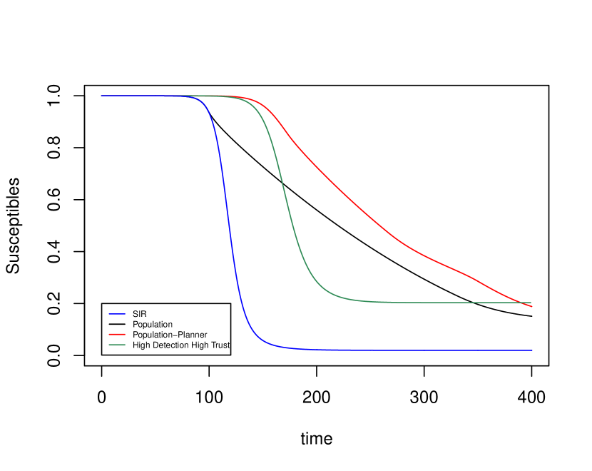
Figure 1: Susceptible fraction for SIR (blue), pure population equilibrium (black), planner-population equilibrium (red) and population equilbirium with high detection & trust (green).

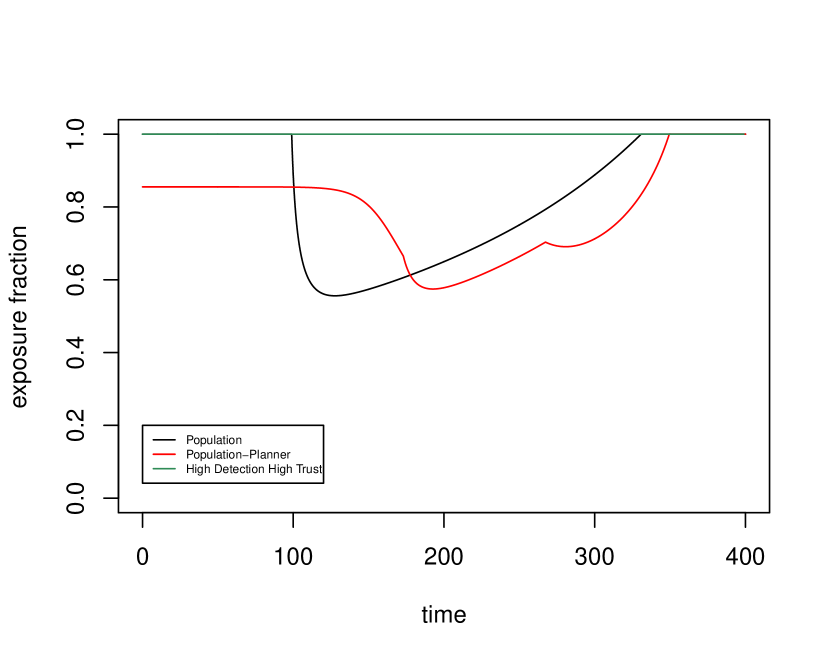
Figure 2: Exposure strategies for cases shown in figure 1.

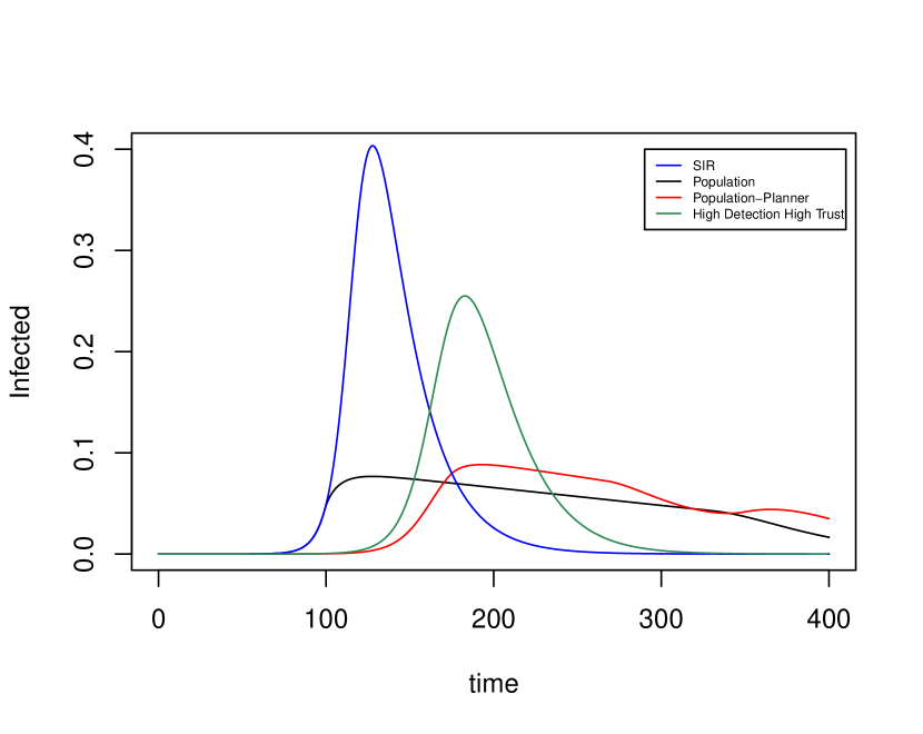
Figure 3: Infection fraction for cases shown in figure 1.

In figures 1, 2 and 3, we plot the susceptible fraction, exposure and infected fraction, respectively, versus time. SIR (blue) shows an exponential decrease in susceptibles at peak infection with almost no susceptibles remaining at the end. This is the worst case scenario- no social distancing, no detection, no quarantining and no planner control. It has the highest peak infection whose onset is advanced compared to other scenarios.

The case with population equilibrium (black) shows a prolonged infection peak with much slower decrease in susceptible numbers (vis-a-vis SIR). From figure 2 it is clear the population starts to socially distance as the infection numbers increase and only stops doing so when it is close to the vaccine arrival time (T).

In the case with planner control (red) the planner initially sets a moderate threshold (see figure 2) to control the spread of the disease. This results in a delayed infection peak. As the infection numbers inevitably rise the population voluntarily reduce exposure below even the planner’s threshold. This results in the peak infection becoming plateaued in a manner similar to population equilibrium. The social distancing and thresholding is gradually reduced as we approach the vaccine arrival (which is assumed to instantly stop the infection). Compared to the population equilibrium case the peak infection is delayed and the economic impact (as measured by exposure time) is reduced.

The case with high detection ($\eta=1$) and high trust ($\kappa=1$) leads to significantly lower peak than SIR but unlike the population or population planner cases the peak is not prolonged (though the peak infection itself is higher). There is no social distancing due to high levels of trust, detection and quarantining. The total susceptible surviving at the end is similar to population or population-planner case. This seems to be the most preferable case where the peak infection is delayed and not prolonged and the economic impact minimal assuming the higher peak infection can be managed.

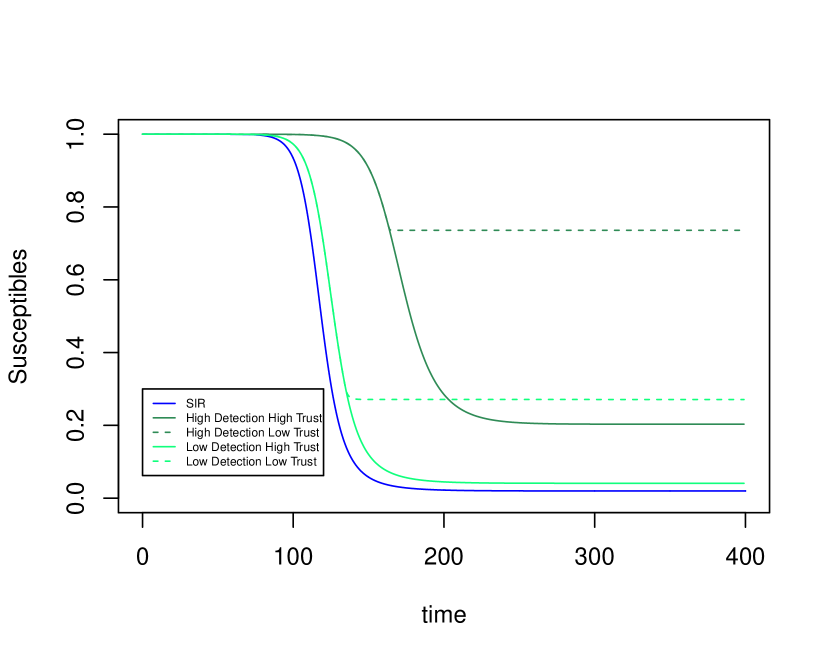
Figure 4: Susceptible fraction for SIR (blue), population equilibrium with high detection & trust (dark green), with high detection & low trust (dashed dark-green), with low detection & high trust (light green) and low detection & low trust (dashed light green).

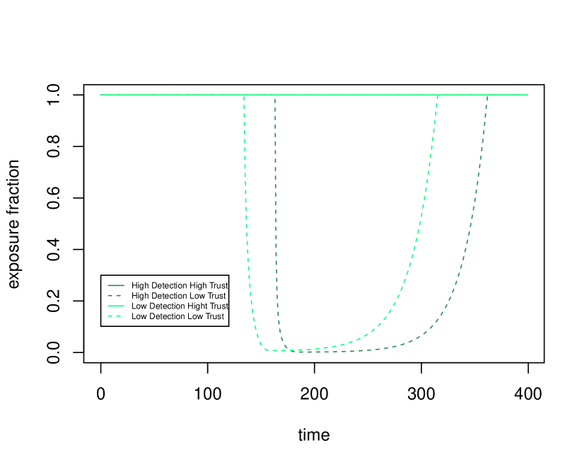
Figure 5: Exposure strategies for cases shown in figure 4.

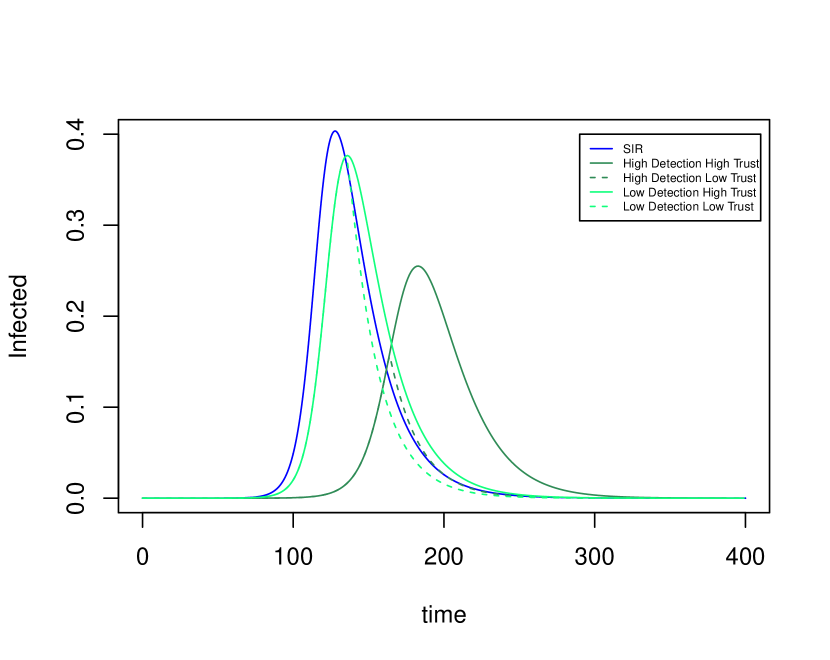
Figure 6: Infection fraction for cases shown in figure 4.

In figures 4, 5 and 6, we plot the effects of different detection rates ($\eta$) and trust parameters ($\kappa$) on the spread of disease. We have already discussed the case with high detection and high trust in the paragraph above. In the case where the detection rates are high ($\eta=1$) but trust ($\kappa=32$) is low (dashed dark green), then we observe that (see figure 5) as soon as infected numbers peak the population completely reduces exposure to zero. This completely stops the disease spread. This is due to the low trust in the detected numbers. The population believes the planner is doing a poor job of the detection even though in reality the detection rates are high. This leads to unnecessary loss of exposure benefits.

In the low detection ($\eta=5$) but high trust ($\kappa=1$) (light green) case, the disease spread curve is very close to the SIR situation. This is expected since in this case there is poor detection and yet the population trusts the detected numbers are an accurate measure of disease spread. This leads to the undetected infected comprising the entirety of the infected numbers while the population seeing the low detection numbers chooses not to socially distance. This is similar to the SIR situation where there is no planner control nor any social distancing.

Finally in the low detection ($\eta=5$) and low trust ($\kappa=32$) (dashed light green) case, just as in the high detection low trust case, the population reduces exposure completely as soon as the infection numbers start to peak. However, compared to the high detection setting the total infected numbers is higher because most of the infected aren’t detected and help spread the disease.

The various comparisons seem to suggest ideally for controlling disease spread one needs to have high detection rates with transparency in the reported numbers so that the population has confidence in the reported numbers. If the detection numbers are low and the planner tries to underplay the poor detection it could result in the worst possible scenario- an unmitigated disease spread which could stress the medical resources at peak infection. In practice, it is often difficult to achieve very high detection rates due to asymptomatic carriers, testing errors etc. and hence must be combined with some moderate amount of planner control in form of lockdowns and imposing social restrictions. The population also has an important role to play by voluntarily reducing exposure and other NPIs (wearing masks, sanitisation, adhering to restrictions etc.). The role of trust/confidence in the reported numbers is demonstrated - too little confidence can lead to a panic, societal intermingling can stop leading to other adverse effects like economic collpase and too much confidence can lead to scenarios where the confidence is unfounded, leading to unmitigated spread of the dissease.

V CONCLUSION

A unified game theoretic framework incorporating the interventions of a planner, behavioral choices of individuals, detection rates and trust in reported numbers has been developed. Both the planner and population begin to favor moderate social distancing when the infection numbers begin to peak. The detection and the subsequent trust in these reported numbers also play crucial role in the spread of disease. Too little detection coupled with unfounded confidence can lead to an unmitigated spread of the disease while too little confidence when the detection is reasonably high leads to unnecessary loss of economic activity. Simulation results supporting these conclusions are presented.

VI ACKNOWLEDGMENTS

The author acknowledges the useful discussions he had with Prof. Sandeep K. Juneja on this topic. This work was supported by the Department of Atomic Energy, Government of India, under project no. RTI4001.

Appendix A
Proof of (6).
In what follows we have set $P_{t}:=\mathbb{P}(\tau>t)$. Define $Z_{t}$, $\forall t\in[0,T]$ as follows :

$$Z_{t} :=\mathbb{E}\bigg{[}\int\displaylimits_{t}^{\tau\wedge T}Bg_{s}ds-(C+R)\mbox{1{1}}_{\{\tau\leq T\}}\bigg{|}\tau>t\bigg{]}$$

$$=\int\displaylimits_{0}^{\tau\wedge T-t}g_{r+t}\frac{P_{t+r}}{P_{t}}[B-\beta(C+R)g_{r+t}I_{r+t}]dr$$

Observe that $Z_{0}$ is the loss functional $J_{\alpha}$. For any time $t<T$ we have:

$$Z_{0}= \mathbb{E}\bigg{[}\int\displaylimits_{0}^{\tau\wedge T}Bg_{s}ds-(C+R)\mbox{1{1}}_{\{\tau\leq T\}}\bigg{]}$$

$$= \mathbb{E}\bigg{[}(\int\displaylimits_{0}^{\tau\wedge T}Bg_{s}ds-(C+R)\mbox{1{1}}_{\{\tau\leq T\}})\mbox{1{1}}_{\{\tau\leq t\}}\bigg{]}+$$

$$\mathbb{E}\bigg{[}\int\displaylimits_{0}^{\tau\wedge T}Bf_{s}ds-(C+R)\mbox{1{1}}_{\{\tau\leq T\}}\bigg{|}\tau>t\bigg{]}P_{t}$$

$$= H_{t}+P_{t}(\int_{0}^{t}Bg_{s}ds)+P_{t}Z_{t}$$

where $H_{t}$ is defined as

$$H_{t}:=\mathbb{E}[(\int_{0}^{\tau\wedge T}Bg_{s}ds-(C+R)\mbox{1{1}}_{\{\tau\leq T\}})\mbox{1{1}}_{\{\tau\leq t\}}]$$

Now since time $t$ was arbitrary we can write the same expression for $t+\Delta t<T$ with $\Delta t>0$. Thus:

$$H_{t}+P_{t}(\int\displaylimits_{0}^{t}Bf_{s}ds)+P_{t}Z_{t}= H_{t+\Delta t}+P_{t+\Delta t}(\int\displaylimits_{0}^{t+\Delta t}Bg_{s}ds)$$

$$+P_{t+\Delta t}Z_{t+\Delta t}$$

Solving for $Z_{t}$ we get:

$$Z_{t} =\frac{(H_{t+\Delta t}-H_{t})}{P_{t}}+\bigg{[}\frac{P_{t+\Delta t}}{P_{t}}(\int\displaylimits_{0}^{t+\Delta t}Bg_{s}ds)-\int_{0}^{t}Bg_{s}ds\bigg{]}$$

$$+\frac{P_{t+\Delta t}}{P_{t}}Z_{t+\Delta t}$$

Plugging in the definition of $H_{t}$ and doing some straightforward but tedious algebra we get:

$$Z_{t}= \frac{\mathbb{E}[\mbox{1{1}}_{\{t<\tau\leq t+\Delta t\}}\int_{t}^{\tau}Bg_{s}ds]}{P_{t}}+\frac{P_{t+\Delta t}}{P_{t}}(\int_{t}^{t+\Delta t}Bg_{s}ds)$$

$$+\frac{P_{t+\Delta t}}{P_{t}}Z_{t+\Delta t}-(C+R)\frac{\mathbb{E}_{\tau}[\mbox{1{1}}_{\{t<\tau\leq t+\Delta t\}}]}{P_{t}}$$

Zubtracting $Z_{t+\Delta t}$ on both sides and dividing by $\Delta t$ we get:

$$\underbrace{\frac{Z_{t}-Z_{t+\Delta t}}{\Delta t}}_{\text{A}}=\underbrace{\frac{\mathbb{E}[\mbox{1{1}}_{\{t<\tau\leq t+\Delta t\}}\int_{t}^{\tau}Bg_{s}ds]}{P_{t}\Delta t}}_{\text{B}}+\underbrace{\bigg{[}\frac{\frac{P_{t+\Delta t}}{P_{t}}-1}{\Delta t}\bigg{]}Z_{t+\Delta t}}_{\text{C}}$$

$$+\underbrace{\frac{P_{t+\Delta t}}{P_{t}}Z_{t+\Delta t}\bigg{[}\frac{\int_{t}^{t+\Delta t}Bg_{s}ds}{\Delta t}\bigg{]}}_{\text{D}}-\underbrace{(C+R)\frac{\mathbb{E}[\mbox{1{1}}_{\{t<\tau\leq t+\Delta t\}}]}{P_{t}\Delta t}}_{\text{E}}$$

We will analyse this in the limit $\Delta t\to 0$ term by term. For term $B$ we observe that:

$$\mathbb{E}[\mbox{1{1}}_{\{t<\tau\leq t+\Delta t\}}\int_{t}^{\tau}Bg_{s}ds] \leq B\mathbb{E}[\mbox{1{1}}_{\{t<\tau\leq t+\Delta t\}}(\tau-t)]$$

$$\leq B\mathbb{P}(t<\tau\leq t+\Delta t)\Delta t$$

Hence:

$$\underset{\Delta t\to 0}{lim}B=0$$

For term C we note that $\frac{1}{P_{t}}\frac{dP_{t}}{dt}=\underset{\Delta t\to 0}{lim}\frac{\mathbb{P}(\tau\leq t+\Delta t|\tau>t)}{\Delta t}$ to get:

$$\underset{\Delta t\to 0}{lim}C=-(\beta g_{t}^{2}I_{t})Z_{t}$$

For term D from Mean Value Theorem for integrals we have for some $t\leq s^{\prime}<t+\Delta t$:

$$\frac{\int_{t}^{t+\Delta t}Bg_{s}ds}{\Delta t}=Bg_{s^{\prime}}$$

This combined with continuity of $g_{t}$ and the fact $\mathbb{P}(\tau>t+\Delta t|\tau>t)\to 1$ as $\Delta t\to 0$ gives us :

$$\underset{\Delta t\to 0}{lim}D=Bg_{t}$$

Term E can be evaluated in a manner similar to term C:

$$\underset{\Delta t\to 0}{lim}E=(C+R)\beta g^{2}_{t}I_{t}$$

This shows that the limit in term A exists and is equal to $\frac{dZ_{t}}{dt}$. Hence we have the differential equation:

$$-\frac{dZ_{t}}{dt}=Bg_{t}-\beta g^{2}_{t}I_{t}Z_{t}-(C+R)\beta g^{2}_{t}I_{t}$$

We also observe from definition of $Z_{t}$ that $Z_{T}=0$. This is the same equation as the adjoint variable $\lambda_{t}$ in Theorem 1 with the relation $\lambda_{t}=-Z_{t}-R$.

References

• [1] Kermack, W. O., & McKendrick, A. G. (1927). A contribution to the mathematical theory of epidemics. Proceedings of the royal society of london. Series A, Containing papers of a mathematical and physical character, 115(772), 700-721.
• [2] Brauer, F., Driessche, P. D., & Wu, J. (2008). Lecture notes in mathematical epidemiology. Berlin, Germany. Springer, 75(1), 3-22.
• [3] Beckley, R., Weatherspoon, C., Alexander, M., Chandler, M., Johnson, A., & Bhatt, G. S. (2013). Modeling epidemics with differential equation. Tennessee State University Internal Report.
• [4] Gao, S., Teng, Z., Nieto, J. J., & Torres, A. (2007). Analysis of an SIR epidemic model with pulse vaccination and distributed time delay. Journal of biomedicine & biotechnology, 2007, 64870. https://doi.org/10.1155/2007/64870
• [5] Aldila, D., Nuraini, N., & Soewono, E. (2014). Optimal control problem in preventing of swine flu disease transmission. Applied Mathematical Sciences, (69-72), 3501-3512. https://doi.org/10.12988/ams.2014.44275
• [6] Aldila, D., Götz, T., & Soewono, E. (2013). An optimal control problem arising from a dengue disease transmission model. Mathematical biosciences, 242(1), 9–16. https://doi.org/10.1016/j.mbs.2012.11.014
• [7] Álvarez, F., Argente, D., & Lippi, F. (2020). A Simple Planning Problem for COVID-19 Lockdown. CEPR: International Macroeconomics & Finance (Topic).
• [8] Acemoglu, D., Chernozhukov, V., Werning, I., & Whinston, M. D. (2020). A multi-risk SIR model with optimally targeted lockdown (Vol. 2020). Cambridge, MA: National Bureau of Economic Research.
• [9] Scott R Sheffield, Anna York, Nicole A Swartwood, Alyssa Bilinski, Anne Williamson, and Meagan C Fitzpatrick. (2020). Strict physical distancing may be more efficient: A mathematical argument for making lockdowns count. medRxiv.
• [10] Farboodi, M., Jarosch, G., & Shimer, R. (2021). Internal and external effects of social distancing in a pandemic. Journal of Economic Theory, 196, 105293.
• [11] Toxvaerd, F.M.O, 2020. ”Equilibrium Social Distancing,” Cambridge Working Papers in Economics 2021, Faculty of Economics, University of Cambridge.
• [12] Friesz, T. L. (2010). Dynamic optimization and differential games (Vol. 135). Springer Science & Business Media.
• [13] Göllmann, L., Kern, D. and Maurer, H. (2009), Optimal control problems with delays in state and control variables subject to mixed control–state constraints. Optim. Control Appl. Meth., 30: 341-365. https://doi.org/10.1002/oca.843
• [14] Chachuat, B. (2007). Nonlinear and dynamic optimization: From theory to practice (No. LECTURE).
• [15] Liberzon, D. (2011). Calculus of variations and optimal control theory. Princeton university press.
• [16] Ince, E. L. (1956), Ordinary Differential Equations, New York: Dover Publications.
• [17] Chi, H., Bell, J. & Hassard, B. (1986), Numerical solution of a nonlinear advance-delay-differential equation from nerve conduction theory. J. Math. Biology 24, 583–601. https://doi.org/10.1007/BF00275686
• [18] Keller, H. B. (1976). Numerical Solution of Two Point Boundary Value Problems. United States: Society for Industrial and Applied Mathematics (SIAM, 3600 Market Street, Floor 6, Philadelphia, PA 19104).