KNN-Averaging for Noisy Multi-Objective Optimisation

Abstract

Multi-objective optimisation is a popular approach for finding solutions to complex problems with large search spaces that reliably yields good optimisation results. However, with the rise of cyber-physical systems, emerges a new challenge of noisy fitness functions, whose objective value for a given configuration is non-deterministic, producing varying results on each execution. This leads to an optimisation process that is based on stochastically sampled information, ultimately favouring solutions with fitness values that have co-incidentally high outlier noise. In turn, the results are unfaithful due to their large discrepancies between sampled and expectable objective values. Motivated by our work on noisy automated driving systems, we present the results of our ongoing research to counteract the effect of noisy fitness functions without requiring repeated executions of each solution. Our method kNN-Avg identifies the k-nearest neighbours of a solution point and uses the weighted average value as a surrogate for its actually sampled fitness. We demonstrate the viability of kNN-Avg on common benchmark problems and show that it produces comparably good solutions whose fitness values are closer to the expected value.

1 Introduction

In the past, multi-objective optimisation (MOO) has proven to be a robust and reliable means in the software engineering toolbox. Through iterative modifications of existing problem solutions, the algorithms try to approach optimal valuations. A fitness function evaluates the quality of each individual solution in one generation so that the best individuals can be used to guide the next generation. After reaching a target fitness or a given number of generations, the algorithm terminates and yields the best solutions found.

MOO algorithms such as genetic algorithms (GAs) have been successfully applied to various optimisation problems, ranging from evolutionary design [3], biological and chemical modelling [6], to artificial intelligence [14]. MOO are particularly well-suited for modern cyber-physical systems (CPSs) and internet of things (IoT) applications, given the high-dimensional search space, where combinatorial testing and exhaustive verification reach their limits. When applied to CPSs, however, a new difficulty arises. Many such systems suffer from sensor errors and measurement noise. Similarly, with growing component numbers, inter-process communication causes non-deterministic behaviour due to message delays and synchronisation time variations. As the messages’ processing times differ at runtime, noisy behaviour emerges [1]. Due to the noise, the reported fitness and the actually expected value (the mean over several evaluations) might vastly differ, leading to distrust of the method.

One of our lines of work is to identify problematic behaviour in automated driving systems (ADSs) by creating driving scenarios through map design changes (e.g. road shape), altering traffic participants (vehicles and pedestrians) and driving behaviour (e.g. aggressiveness). However, due to noisy inter-process communication, repeated executions of the same scenario can lead to differing observations, s.t. the distance between two cars may vary up to several meters. In other words, in our search for consistent collision scenarios, outliers for typical non-crash scenarios might be identified as crash scenarios. This leads to volatile test scenarios, non-reproducible crash reports, and otherwise inconsistent scenario design.

Evidently, a naive fix is to repeatedly run each configuration and select the mean or median fitness value to check for robustness. However, in our setting this is not possible, as a typical simulation takes 1 to 2 minutes. Assuming 1000 total optimisation steps, re-evaluating every run five more times adds some 80 to 160 hours of simulation time to each individual scenario search, rendering this method infeasible for broad application.

In this paper, we introduce kNN-averaging to overcome the problem of lacking fitness robustness and outliers in noisy optimisation problems and provide our advances on common, theoretical benchmark problems. Our method kNN-Avg uses the k-nearest neighbours (kNN) ($k$ being a hyper-parameter) to compute the fitness value and thereby reduce the noise. We show that in a typical setting without noise mitigation, GAs tend to predict outlier values and that kNN-Avg helps to overcome this problem, making the found solutions more robust. To evaluate our approach, we adapt three well-known MOO benchmarks to noisy environments and quantify our results using common quality indicators (QIs).

2 Multi-Objective Optimisation & Genetic Algorithms

Multi-objective optimisation problems are a family of problems that aim to optimise multiple function values. Formally, the goal is to find the minimum parameter (a.k.a. variable) values $\vec{x}\in\mathbb{X}$ such that the function values of a vector of objective functions $f$ are minimised. $\mathbb{X}\subseteq\mathbb{R}^{n}$ represents the solution space, i.e. the input to $f$, and relates to the scenario parameters that we defined above. $\vec{x}$ is called a solution.

$$\min_{\vec{x}\in\mathbb{X}}f(\vec{x})=\{f_{1}(x),\dots,f_{m}(x)\},\forall i\in\{1,\dots,m\},f_{i}:\mathbb{X}\rightarrow\mathbb{R}$$ (1)

The output $f(\vec{x})\in\mathbb{Y}$ is called the objective value of $\vec{x}$; $\mathbb{Y}\subseteq\mathbb{R}^{m}$ being the objective space. An optimisation problem is called multi-objective if $m>1$.

While for single-objective optimisation problems, a solution leading to a smaller objective value than another is considered better (dominant), this notion is not as clear in the MOO setting. Here, given two solutions $\vec{x}_{a},\vec{x}_{b}\in\mathbb{X}$, we say that $\vec{x}_{a}$ dominates $\vec{x}_{b}$ ($\vec{x}_{a}\prec\vec{x}_{b}$) iff $\forall i\in\{1,\dots,n\},f_{i}(\vec{x}_{a})\leqslant f_{i}(\vec{x}_{b})\wedge\exists j\in\{1,\dots,n\}\colon f_{j}(\vec{x}_{a})<f_{j}(\vec{x}_{b})$.

A solution is Pareto optimal iff there is no other solution that dominates it. A Pareto set $PS^{*}\in\mathbb{X}$ is the set of all Pareto optimal solutions, a Pareto-front PF^∗ is the image of the Pareto set in the objective space. Roughly speaking, PS^∗ is the set of solutions where we cannot optimise one $f_{i}$-dimension without having to reduce optimality in another one. This means, however, that there might be numerous Pareto optimal solutions for some problems. Fig. 1(a) shows a solution set for the benchmark problem ZDT1 [17] alongside its Pareto front PF^∗. Note that each value of the solution set is Pareto optimal.

Quality Indicators (QI) QIs allow an estimation of a MOO’s performance. Numerous QIs have been proposed [13]. In this paper, we focus on two of the most common ones.

Hypervolume (HV) It calculates the hypervolume between a given reference point in the objective space and each of the solutions’ objective values. Typically, it uses a reference that is worse than all expected objective values. Thus, the HV increases as the solutions approach the Pareto-optimality.

Inverse generational distance (IGD) IGD calculates the average Euclidean distance from each PF^∗-point to its closest solution. IGD decreases when approaching PF^∗.

Genetic algorithms (GAs) GAs [7] are a subfamily of evolutionary algorithms (EAs) whose working principle is based on the iterative creation of populations (sets of solutions, a.k.a. generations). An initial population can be created from random samples, and all following generations are based on the best candidates from their predecessors. This is achieved by ranking the solutions according to their fitness values $f(\vec{x})$ and applying operators to the best ones: selection keeps the good ones, crossover produces new solutions by “mating” two others, and mutation creates a slightly altered version of an existing one.

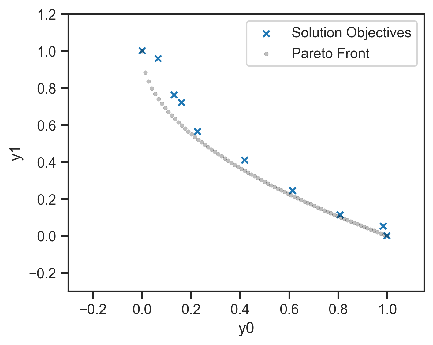
(a) A solution set for the MOO problem ZDT1 and optimal Pareto front PF^∗

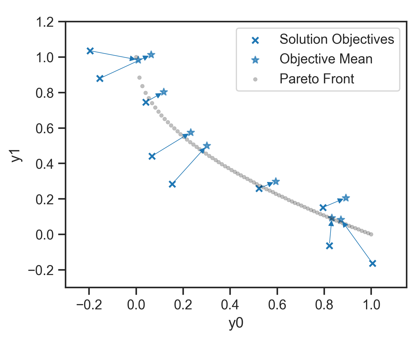
(b) Noisy ZDT1_σ=0.1 objectives after optimisation, and the solutions’ mean objectives.

Figure 1: Left: search problem without noise; Right: Noisy search problem

3 Noisy MOO and K-Nearest-Neighbour Averaging

We use the term noisy MOO to refer to problems whose fitness function $f(x)$ is non-deterministic. The formal problem statement, introduced in Eq. 1, can be updated to

$$\min_{\vec{x}\in X}f(\vec{x})=\{f_{1}(\vec{x})+\delta_{1},\dots,f_{m}(\vec{x})+\delta_{m}\}$$ (2)

where each $\delta_{i}$ is a noise value sampled from a distribution. In many real-world systems, as well as common benchmark studies, the noise in the system is Gaussian-distributed [11]. To make our results comparable, we follow this lead, and therefore, for the rest of this paper, we fix that $\delta_{i}$ is sampled from a normal distribution with mean $\mu=0$ and a standard deviation $\sigma$. We use $\sigma$ as a variable and alter it depending on the particular benchmark. For noisy systems, we indicate the problem’s noise $\sigma$-parameter as subscript, e.g. ZDT1_σ=0.1, as in Fig. 1(b).

Noise Effect

When introducing noise into an optimisation problem, the effect is that PF^∗ no longer represents the optimal objective values but instead marks the mean objective values for PS^∗. Given a solution $s\in PS^{*}$ and high enough repetitions, the mean value should be placed near the solution’s expected (non-noisy) objective.

Interestingly though, when executing a GA on such a problem, the typical result (see also  [10]) is that the algorithm computes a set of solutions that approaches PS^∗, but predicts objective values with high negative noise, falsely indicating extraordinarily good fitness values. Thus, in the final solution set $\mathit{S}$, the GA “pushes” the reported fitness value far beyond PF^∗, as can be seen in Fig. 1(b). The result is that the objective values do not match the actual distributions of the solutions’ expected mean objective values, and in fact over-estimate the quality of the $\mathit{S}$. Fig. 1(b) displays both the sampled solutions’ objective values as well as these solutions’ mean objective values. $\mathit{S}$ was obtained by running 100 iterations of the GA-optimisation of the noisy ZDT1_σ=0.1 problem. In the figure, we can observe several properties:

1. The objective values of the found non-dominated solution set $\mathit{S}$ (marked by crosses) actually significantly surpass PF^∗.

2. By evaluating $s\in\mathit{S}$ repeatedly (or by removing the noise), we reveal the actual mean objective values, i.e. the centre points of the noisy objective distributions (marked by asterisks).

3. Some of the mean objective values are clearly dominated by others. Thus, evaluating $s\in\mathit{S}$ will likely lead to non-dominated solutions.

4. The observed objective values are typically based on large noise values, i.e. they are outliers.

5. On average, the distance between observed objectives and the mean objectives (indicated by the arrows) is rather large — even exceeding $\sigma$. Thus, the obtained solutions’ fitness is misleading.

6. Even though the solutions’ objective values do not match the mean objective values, the solutions’ mean objective values approach PF^∗. This means that while we cannot expect fitness values to be as good as predicted by the optimisation process, on average the solution values will still be good.

7. It appears that the noise causes the search to stop further improvement, since outlier noise suggests the greatest possible fitness was already reached.

Ideally, the solutions’ mean objectives would align with PF^∗, s.t. this result would produce the best fitness on average.

Research Goal

Indeed, in Fig. 1 where we know that the noise (induced by $\sigma$) is constant throughout the search space and as we know PF^∗, we can easily see the offset. However, for unknown problems, problems with potentially fluctuating noise magnitudes or similar situations, we should aim to produce solutions whose sampled objective values are close to the mean objective values. This way, we know that the individuals’ objectives are reliable and the obtained values representative. In other words, our goal is to push the crosses in Fig. 1(b) closer towards the asterisks, while keeping the asterisks close to the ideal Pareto front PF^∗.

Mean Offset $\Delta f$

We introduce a new measure $\Delta f$ to calculate the mean Euclidean distance between $\mathit{S}$’s reported objective values $f(s),s\in\mathit{S}$ — as obtained by the search — and the mean expected objective values $\tilde{f}(s)$ — obtained e.g. by taking the mean of repeated invocations of $f$ on $s$. $\Delta f$ thus measures the average length of the arrows in Fig. 1(b). The rest of this section describe our method which leverages the weighted average of the k-nearest neighbours to robustify the sampling process and reduce $\Delta f$.

$$\Delta f=\frac{\sum_{s\in\mathit{S}}\sqrt{(f(s)-\tilde{f}(s))^{2}}}{\mid\mathit{S}\mid}$$ (3)

3.1 KNN-Averaging

Theoretically, inputs to noisy fitness functions can be repeatedly evaluated and the sampled values averaged. Given high enough repetition frequency, this mean objective value should approach the actual expectation value. The problem of this method is the cost involved in the re-sampling of values, which can be significant for complex systems such as automated driving simulators, even rendering the search effectively infeasible.

Our novel approach kNN-Avg aims to approximate the re-sampling process and decrease the objective values noise, without actually performing the costly repeated sampling. Our concept is based on the hypothesis that solutions that are close to one another in the solution space will produce similarly distributed objective values. Thus, the goal is to identify previously evaluated solutions close to the currently sampled point and use their fitness values to help decrease the impact of outliers.

Standardised Euclidean Distance

Euclidean distance (ED)is one of the go-to distance measures when it comes to evaluating the proximity of multi-dimensional data points, providing the “shortest direct distance” between two points. On closer inspection, however, we notice that often the values depend on the individual dimensions’ units. Thus, the Euclidean distance of values expressed in kilometres is vastly different than the one in metres. Moreover, the measure is not robust against large magnitude differences. When one dimension expresses vehicle size in metres, but the other travelled distances in kilometres, the second dimension will probably dominate the measure.

Our goal is thus to use a measure that normalises over the actually used search space to avoid such tilting of the distance measure. We therefore use the standardised Euclidean distance (SED), which normalises the values by relating the value difference to the dimension’s variance within the total set of values in that dimension.

Definition 1 (Standardised Euclidean distance)

The standardised Euclidean distance (SED)of two vectors is the square-root of the sum of the squared element-wise difference divided by the dimension’s variance $\sigma_{i}^{2}$:

$$\mathit{sed}(\vec{x}_{1},\vec{x}_{2})=\sqrt{\sum_{i=1}^{N}{\frac{(x_{1,i}-x_{2,i})^{2}}{\sigma_{i}^{2}}}},$$ (4)

Note that the difference to the “common” Euclidean distance, i.e. the division by the dimension’s variance $\sigma_{i}^{2}$, places each dimension in relation to the global value spread. This robustifies standardised Euclidean distance (SED) against magnitude changes in the solution space and we can—in theory—even change, e.g. the units from km to m.

3.2 Hyper-Parameters of kNN-Avg

Next to the choice of distance measure, the kNN-Avg algorithm offers several other configuration parameters. Here, we will briefly outline some of the questions that have to be answered before executing the algorithm.

How big should $k$ be?

Intuitively, we might want to include as many neighbours as possible to minimise the noise factor. The problem is, however, that higher $k$-values take more distant neighbours into account, which are less similar to the solution under investigation. Typically, the answer also depends on the shape of the search space and the standard deviation of the noise.

When does a neighbour stop being “near”?

Especially at the beginning of the search when the sampling history is still sparse, a kNN algorithm without a cutoff limit might select rather distant neighbours for the averaging. To avoid this, we use a maximum distance $\mathtt{MD}$ to limit the kNN search to the local neighbourhood.

Should close neighbours weigh more?

By default, our hypothesis is that close neighbours produce more similar value distributions than those further away. Based on an informal initial exploration, our algorithm uses the squared SED to decrease a neighbours impact weight. Nonetheless, this raises the question as to how those weights are shaped in general. We leave this more general question as future works.

We performed an upfront literature search, but it did not reveal conclusive answers or best practices for good choices on these hyper-parameter values. Thus, $k$ and maximum distance $\mathtt{MD}$ are left variable. The experiments section explores the relationship between these hyper-parameter values and the performance of the MOO process. The weight measure on the other hand was fixed as the inverse-square of the SED. Before choosing squared, we also experimented with linear and uniform distance weights, but did not observe as good results.

3.3 Algorithm

Based on the kNN-Avg approach and the identified hyper-parameters we implemented the algorithm, as displayed in LABEL:lst:knn-algorithm.

Listing 1: KNN-Evaluation algorithm in (Python-ish) pseudo-code

⬇

1"""Store the solutions with actually sampled values."""

2HISTORY = list() # global store of solutions

3"""Calculate KNN-averaged objectives for a list of solutions."""

4def knn_evaluate(population: List[Solution], KNN: int, MAX_DIST: float) -> List[Solution]:

5 # standard evaluation of each solution; add results to the history

6 sampled = [evaluate(solution) for solution in population]

7 HISTORY.extend(sampled)

8 # calculates the list of variance (one per variable dimension)

9 variances = get_variances(HISTORY)

10 # calculate solutions with KNN-averaged objectives

11 knn_solutions = list()

12 for solution in population:

13 # store a map of solution-to-SED

14 distances={other:SED(solution, other, variances) for other in HISTORY}

15 # remove those that are larger than MAX_DISTANCE

16 knn = {sol: val for sol, val in knn.items() if val <= MAX_DIST)

17 # sort by distance and limit to KNN values

18 knn = distances.sort(by=distances.values())[:KNN]

19 # calculate the weights as the square of distance values;

20 # negate and add MAX_DIST so sol itself is largest

21 weights = math.square(knn.values()) ^∗ -1 + MAX_DIST

22 objs = [sol.objs for sol in knn]

23 avgs = weighted_mean(objs, weights, column=True)

24 # append to the list of returned solutions

25 knn_solutions.append(Solution(solution.vars, avgs))

26 return knn_solutions

27

28"""Data-class for solutions and corresponding objective values."""

29class Solution(object):

30 vars = list() # variables will be filled by the GA

31 objs = list() # objectives are filled by us

The algorithm is presented in a Python-like pseudo-language and makes references to “mock” functions such as get_variances. The actual implementation uses common Python libraries such as numpy and pandas.

The listing’s knn_evaluate-function is meant to replace the native evaluate-function of a GA implementation. It is called once per generation and takes as input a list of solutions, as well as the KNN and MAX_DIST hyper-parameters. The output is a list of Solution objects, each containing variables and kNN-averaged objective values. Specifically, each population cycles through the following steps:

1. The algorithm first invokes the (noisy) default evaluate method (L 6). This can be e.g. the triggering of a simulator.

2. After this evaluation, the solutions (now containing the sampling results) are added to the global HISTORY (L 2 and L 7).

3. In the next step, the variances are calculated for each solution dimension separately (L 9). The variances are later used to calculate the SED.

4. Then, each solution iterates through the following steps:

   1. Calculate the solution’s SEDs to each other solution in the global history — including itself and all other newly generated solutions (L 14).

   2. Select all solutions closer than MAX_DIST (L 16).

   3. Sort solutions by the SED and only keep the k-nearest neighbours (L 18).

   4. Calculate the weights of each knn as the negative square of its SED (L 21). Then add MAX_DIST to make all values positive.

   5. Calculate the objective values as the weighted mean values. Note that since objectives is a two-dimensional list, we have to specify column-wise aggregation, such that each dimension is averaged separately (L 22 – 23). The solution variables and averaged objectives are used to append a new Solution to the list that will be returned to the algorithm.

kNN-Avg Effect

The effect of the algorithm is visualised in Fig. 2. It shows the kNN-Avg approach at the evaluation of the 25th generation of a search problem. The evaluation history is shown as coloured crosses. Red dots display the sampled objective values, arrows indicate the corresponding objective values after kNN-Avg (red crosses).

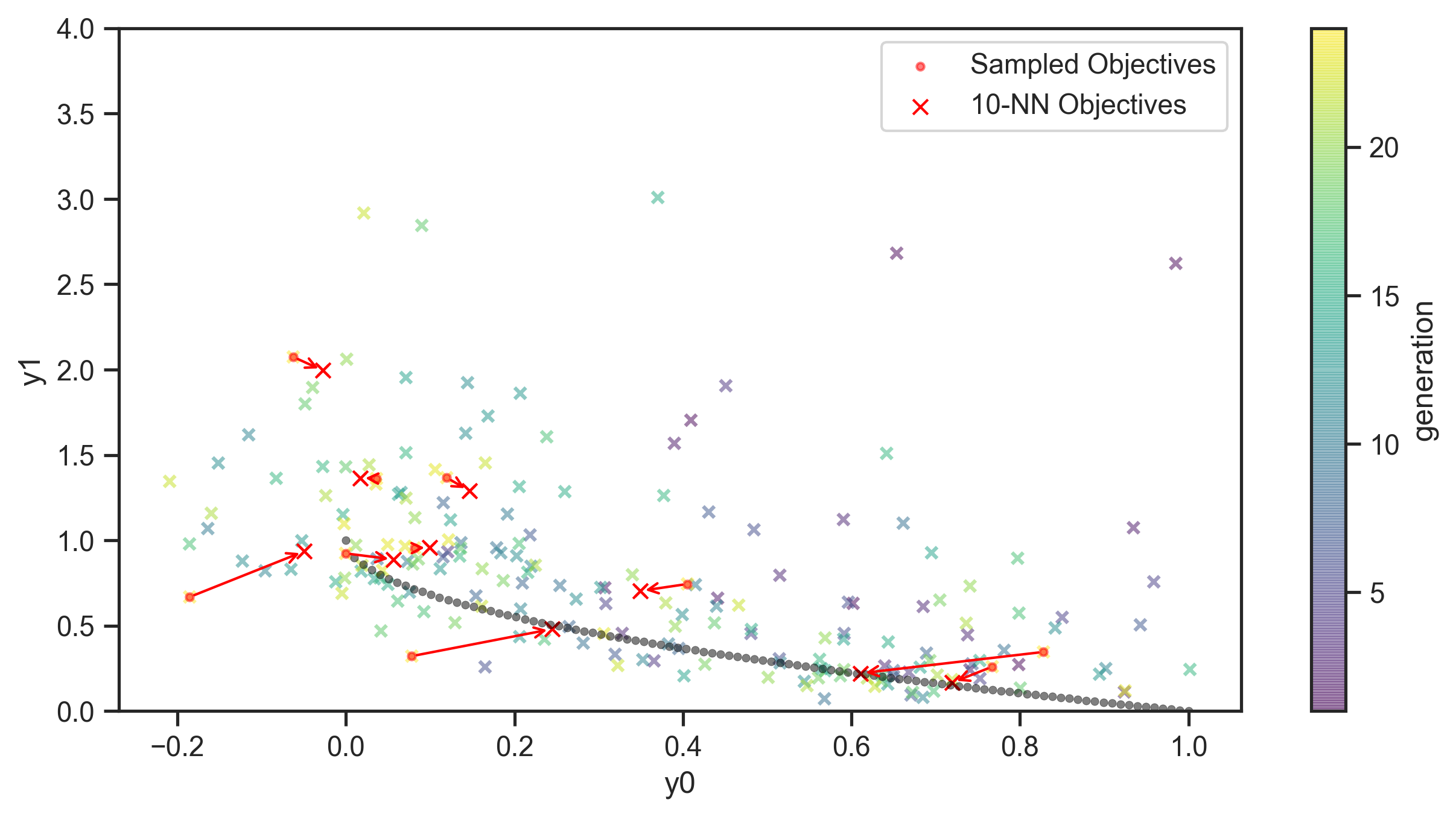
Figure 2: 10-NN Averaging at Generation #25 for ZDT1_σ=0.1. Arrows connect sampled and respective 10-NN-averaged objective values.

4 Evaluation

This section describes the experiments and analyses we performed to answer the following research questions (RQs):

• RQ1: Can kNN-Avg mitigate the outlier-effect of noisy MOO and bring the reported and mean objective values closer together (i.e. reduce $\Delta f$)?

• RQ2: How do the solutions of kNN-Avg compare to those of the baseline in terms of optimality (measured by quality indicators (QIs))?

• RQ3: Does the level of noise have an impact on whether kNN-Avg is able to produce good results?

• RQ4: What influence does the choice of hyper-parameters have on the efficiency of the approach?

4.0.1 Experimental Setup

To evaluate the kNN-Avg method, we implemented a set of noisy benchmarks. The implementation is based on the pymoo Python library [4], which provides a flexible framework for evaluation of MOO problems and algorithms.

For the kNN-Avg evaluation, we developed a KNNAvgMixin-wrapper that we can dynamically add to existing pymoo problems. The wrapper serves two purposes: First, it modifies the wrapped problem and artificially injects noise into the evaluated solutions. Second, it implements the kNN-Avg algorithm to counteract the effects of the noise. The wrapper also stores the full evaluation history and adds data logging for our analysis. It can be flexibly added to existing benchmark problems, e.g. those already available in pymoo.

Using this class, we ran experiments on three benchmark problems: ZDT1, ZDT2 and ZDT3[17]. These artificial MOO benchmarks aim to minimise two-function objectives, based on a variable number of up to 30 inputs. In total, we selected six individual settings with multiple values each, to avoid biasing our algorithm and also obtain an overview of the influence of various hyper-parameters (RQ4). Following guidelines [2], we executed 30 repetitions in each setting to avoid statistical fluctuations and gain enough data for our later analysis. Table 1 displays the experiment settings and the values that each one may take. The total number of experimental settings is given by the Cartesian product of the settings’ values. In total, we executed $67{,}500$ individual optimisation runs.

As MOO method we use NSGA-II, configured with a random initial population, simulated binary crossover (probability 0.9) and polynomial mutation (probability 1.0). The search was run for 100 generations using population size 10 or 20 (see Table 1).

Table 1: Configurations of benchmarks and search algorithms

Label	Values	Comment
Problem	ZDT1, ZDT2, ZDT3	Benchmark name
Num Variables	2, 4, 10	Benchmark configuration
$\sigma$ (Noise Std. Dev.)	0.00, 0.05, 0.10, 0.25, 0.50	Benchmark Noise
Population Size	10,  20	GA setting
$k$ (Num Neighbours)	10, 25, 50, 100, 1000	kNN-Avg hyper-parameter
$\mathtt{MD}$ maximum distance	0.25, 0.5, 1.0, 2.0, 4.0	kNN-Avg hyper-parameter

4.1 Experimental Results

In order to evaluate the effectiveness of the approach, we proceeded as follows.

For each experiment, we took the set of optimised solutions $\mathit{S}$ as computed by the GA; then for each solution $s\in\mathit{S}$, we computed its “mean” objective value $\tilde{s}$; all solutions $\tilde{s}$ constitute the “adjusted” solution set $\widetilde{\mathit{S}}$. Based thereon, we computed the following metrics: (i) $\Delta f$, the average error in estimation between the objective values of solutions in $\mathit{S}$ and the adjusted ones in $\widetilde{\mathit{S}}$ (see Eq. 3); (ii) $\widetilde{\text{HV}}$and $\widetilde{\text{IGD}}$, the hypervolume and IGD (see § 2) of the mean objectives $\tilde{s}\in\widetilde{\mathit{S}}$.

As an example, Fig. 3 shows $\widetilde{\text{HV}}$, $\widetilde{\text{IGD}}$, and $\Delta f$ for the ZDT1_σ=0.1 experiment with 2 variables, grouped by $k$ and maximum distance $\mathtt{MD}$, i.e. by the hyper-parameters we want to evaluate.

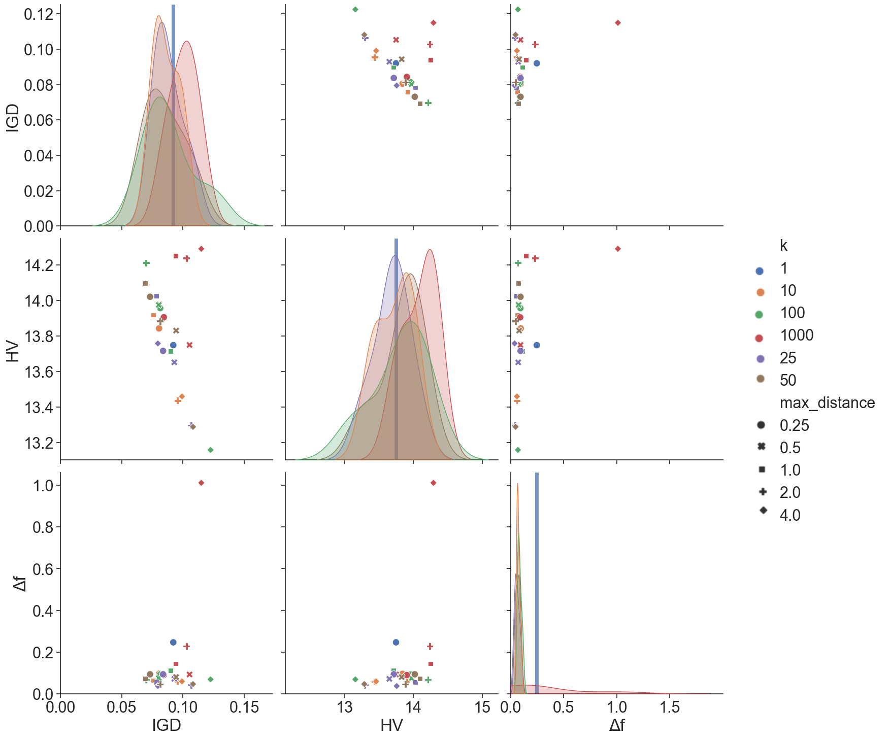
Figure 3: Pairplot of average QI and $\Delta f$ of 30 runs for ZDT1_σ=0.1. Diagonal plots show kernel density estimates. Baseline B ($k=1$; no averaging) is shown as a vertical line.

The plots show the mean results of 30 individual NSGA-II optimisation runs after 100 generations with population size 10. The individual plots show two metrics plotted against each other, while the diagonal plots display the kernel density estimate by $k$ value. Roughly speaking, this is a distribution of where the individual metrics (grouped by $k$) are along the x-axis. Thus, for $\widetilde{\text{IGD}}$ and $\Delta f$, lower (left) is better, while for $\widetilde{\text{HV}}$ higher (right) is advantageous. Further, a flat, wide density shows a spread of values along the axis, while a short, high curve signifies a concentrated values. The baseline represents the standard (non-averaging) noisy MOO, where only the sampled value is chosen without any neighbours(i.e. $k=1$). It is is drawn as vertical blue line. Note, that a comparison to other solution approaches to noisy MOO is left as future work.

We see from the positions of the data points, as well as from the density plots, that for most $k$ values (except $k$$=$$1000$) the $\widetilde{\text{IGD}}$ is lower than B (blue line). For $\widetilde{\text{HV}}$ the value is higher, except $k$$=$$25$. Of particular interest is $\Delta f$, which shows a significant discrepancy between the kNN-Avg evaluations and B, in favour of kNN-Avg.

Thus, we conclude that for this particular benchmark, the kNN-Avg approach produces better results on average than B. We report in the online repository² the detailed analyses of all the 45 benchmarks. In the following, we perform an overall analysis to assess how the proposed approach performs in general.

We calculated the experiments results’ average (grouped by $k$ and $\mathtt{MD}$) and compared them with the results of the baseline B, across all experiment configurations (all combinations of Problem, Num Variables, $\sigma$, and Population size). By following guidelines for conducting experiments with randomised algorithms [2], we compared them using the Wilcoxon signed rank test for the statistical significance (at significance level $\alpha$$=$$0.05$), and the Vargha-Delaney’s Â₁₂ as effect size. Table 2 reports the results of the statistical tests, displaying whether kNN-Avg’s performance is statistically significantly better, equal, or worse than the B’s.

Table 2: Comparison between the kNN-based settings $\mathtt{KNN}_{k}^{\mathtt{MD}}$ and the baseline B.

(a) No noise

App.	$\widetilde{\text{HV}}$	$\widetilde{\text{IGD}}$	$\Delta f$
$\mathtt{KNN}_{10}^{0.25}$	$\equiv$	✗	✗
$\mathtt{KNN}_{10}^{0.5}$	✗	✗	✗
$\mathtt{KNN}_{10}^{1.0}$	✗	✗	✗
$\mathtt{KNN}_{10}^{2.0}$	✗	✗	✗
$\mathtt{KNN}_{10}^{4.0}$	✗	✗	✗
$\mathtt{KNN}_{25}^{0.25}$	✗	✗	✗
$\mathtt{KNN}_{25}^{0.5}$	✗	✗	✗
$\mathtt{KNN}_{25}^{1.0}$	✗	✗	✗
$\mathtt{KNN}_{25}^{2.0}$	✗	✗	✗
$\mathtt{KNN}_{25}^{4.0}$	✗	✗	✗
$\mathtt{KNN}_{50}^{0.25}$	✗	✗	✗
$\mathtt{KNN}_{50}^{0.5}$	✗	✗	✗
$\mathtt{KNN}_{50}^{1.0}$	✗	✗	✗
$\mathtt{KNN}_{50}^{2.0}$	✗	✗	✗
$\mathtt{KNN}_{50}^{4.0}$	✗	✗	✗
$\mathtt{KNN}_{100}^{0.25}$	✗	✗	✗
$\mathtt{KNN}_{100}^{0.5}$	✗	✗	✗
$\mathtt{KNN}_{100}^{1.0}$	✗	✗	✗
$\mathtt{KNN}_{100}^{2.0}$	✗	✗	✗
$\mathtt{KNN}_{100}^{4.0}$	✗	✗	✗
$\mathtt{KNN}_{1000}^{0.25}$	✗	✗	✗
$\mathtt{KNN}_{1000}^{0.5}$	✗	✗	✗
$\mathtt{KNN}_{1000}^{1.0}$	✗	✗	✗
$\mathtt{KNN}_{1000}^{2.0}$	✗	✗	✗
$\mathtt{KNN}_{1000}^{4.0}$	✗	✗	✗

(b) $\sigma={0.05}$

App.	$\widetilde{\text{HV}}$	$\widetilde{\text{IGD}}$	$\Delta f$
$\mathtt{KNN}_{10}^{0.25}$	✗	$\equiv$	✓
$\mathtt{KNN}_{10}^{0.5}$	$\equiv$	$\equiv$	✓
$\mathtt{KNN}_{10}^{1.0}$	✗	✗	✓
$\mathtt{KNN}_{10}^{2.0}$	✗	✗	✓
$\mathtt{KNN}_{10}^{4.0}$	✗	✗	✓
$\mathtt{KNN}_{25}^{0.25}$	$\equiv$	$\equiv$	✓
$\mathtt{KNN}_{25}^{0.5}$	✗	✗	✓
$\mathtt{KNN}_{25}^{1.0}$	✗	✗	✓
$\mathtt{KNN}_{25}^{2.0}$	✗	✗	✓
$\mathtt{KNN}_{25}^{4.0}$	✗	✗	$\equiv$
$\mathtt{KNN}_{50}^{0.25}$	$\equiv$	$\equiv$	✓
$\mathtt{KNN}_{50}^{0.5}$	$\equiv$	$\equiv$	✓
$\mathtt{KNN}_{50}^{1.0}$	✗	✗	✓
$\mathtt{KNN}_{50}^{2.0}$	✗	✗	$\equiv$
$\mathtt{KNN}_{50}^{4.0}$	✗	✗	$\equiv$
$\mathtt{KNN}_{100}^{0.25}$	$\equiv$	$\equiv$	✓
$\mathtt{KNN}_{100}^{0.5}$	✗	✗	✓
$\mathtt{KNN}_{100}^{1.0}$	✗	✗	$\equiv$
$\mathtt{KNN}_{100}^{2.0}$	✗	✗	$\equiv$
$\mathtt{KNN}_{100}^{4.0}$	✗	✗	$\equiv$
$\mathtt{KNN}_{1000}^{0.25}$	$\equiv$	$\equiv$	✓
$\mathtt{KNN}_{1000}^{0.5}$	✗	✗	✓
$\mathtt{KNN}_{1000}^{1.0}$	✗	✗	$\equiv$
$\mathtt{KNN}_{1000}^{2.0}$	✗	✗	✗
$\mathtt{KNN}_{1000}^{4.0}$	✗	✗	✗

(c) $\sigma={0.1}$

App.	$\widetilde{\text{HV}}$	$\widetilde{\text{IGD}}$	$\Delta f$
$\mathtt{KNN}_{10}^{0.25}$	$\equiv$	✓	✓
$\mathtt{KNN}_{10}^{0.5}$	$\equiv$	$\equiv$	✓
$\mathtt{KNN}_{10}^{1.0}$	$\equiv$	$\equiv$	✓
$\mathtt{KNN}_{10}^{2.0}$	✗	✗	✓
$\mathtt{KNN}_{10}^{4.0}$	✗	✗	✓
$\mathtt{KNN}_{25}^{0.25}$	$\equiv$	✓	✓
$\mathtt{KNN}_{25}^{0.5}$	$\equiv$	$\equiv$	✓
$\mathtt{KNN}_{25}^{1.0}$	✗	$\equiv$	✓
$\mathtt{KNN}_{25}^{2.0}$	✗	✗	✓
$\mathtt{KNN}_{25}^{4.0}$	✗	✗	✓
$\mathtt{KNN}_{50}^{0.25}$	$\equiv$	$\equiv$	✓
$\mathtt{KNN}_{50}^{0.5}$	$\equiv$	$\equiv$	✓
$\mathtt{KNN}_{50}^{1.0}$	$\equiv$	$\equiv$	✓
$\mathtt{KNN}_{50}^{2.0}$	✗	✗	✓
$\mathtt{KNN}_{50}^{4.0}$	✗	✗	✓
$\mathtt{KNN}_{100}^{0.25}$	$\equiv$	$\equiv$	✓
$\mathtt{KNN}_{100}^{0.5}$	$\equiv$	$\equiv$	✓
$\mathtt{KNN}_{100}^{1.0}$	$\equiv$	$\equiv$	✓
$\mathtt{KNN}_{100}^{2.0}$	✗	✗	✓
$\mathtt{KNN}_{100}^{4.0}$	✗	✗	✓
$\mathtt{KNN}_{1000}^{0.25}$	$\equiv$	✓	✓
$\mathtt{KNN}_{1000}^{0.5}$	$\equiv$	$\equiv$	✓
$\mathtt{KNN}_{1000}^{1.0}$	$\equiv$	$\equiv$	✓
$\mathtt{KNN}_{1000}^{2.0}$	✗	✗	$\equiv$
$\mathtt{KNN}_{1000}^{4.0}$	✗	✗	✗

(d) $\sigma={0.25}$

App.	$\widetilde{\text{HV}}$	$\widetilde{\text{IGD}}$	$\Delta f$
$\mathtt{KNN}_{10}^{0.25}$	$\equiv$	$\equiv$	✓
$\mathtt{KNN}_{10}^{0.5}$	$\equiv$	✓	✓
$\mathtt{KNN}_{10}^{1.0}$	$\equiv$	✓	✓
$\mathtt{KNN}_{10}^{2.0}$	$\equiv$	✓	✓
$\mathtt{KNN}_{10}^{4.0}$	✗	$\equiv$	✓
$\mathtt{KNN}_{25}^{0.25}$	$\equiv$	$\equiv$	✓
$\mathtt{KNN}_{25}^{0.5}$	$\equiv$	$\equiv$	✓
$\mathtt{KNN}_{25}^{1.0}$	$\equiv$	$\equiv$	✓
$\mathtt{KNN}_{25}^{2.0}$	✗	$\equiv$	✓
$\mathtt{KNN}_{25}^{4.0}$	✗	$\equiv$	✓
$\mathtt{KNN}_{50}^{0.25}$	✓	✓	✓
$\mathtt{KNN}_{50}^{0.5}$	$\equiv$	$\equiv$	✓
$\mathtt{KNN}_{50}^{1.0}$	$\equiv$	✓	✓
$\mathtt{KNN}_{50}^{2.0}$	✗	$\equiv$	✓
$\mathtt{KNN}_{50}^{4.0}$	✗	$\equiv$	✓
$\mathtt{KNN}_{100}^{0.25}$	$\equiv$	✓	✓
$\mathtt{KNN}_{100}^{0.5}$	$\equiv$	✓	✓
$\mathtt{KNN}_{100}^{1.0}$	$\equiv$	✓	✓
$\mathtt{KNN}_{100}^{2.0}$	$\equiv$	$\equiv$	✓
$\mathtt{KNN}_{100}^{4.0}$	✗	$\equiv$	✓
$\mathtt{KNN}_{1000}^{0.25}$	$\equiv$	✓	✓
$\mathtt{KNN}_{1000}^{0.5}$	$\equiv$	✓	✓
$\mathtt{KNN}_{1000}^{1.0}$	$\equiv$	✓	✓
$\mathtt{KNN}_{1000}^{2.0}$	$\equiv$	✓	✓
$\mathtt{KNN}_{1000}^{4.0}$	$\equiv$	$\equiv$	✓

(e) $\sigma={0.5}$

App.	$\widetilde{\text{HV}}$	$\widetilde{\text{IGD}}$	$\Delta f$
$\mathtt{KNN}_{10}^{0.25}$	$\equiv$	$\equiv$	✓
$\mathtt{KNN}_{10}^{0.5}$	$\equiv$	$\equiv$	✓
$\mathtt{KNN}_{10}^{1.0}$	$\equiv$	$\equiv$	✓
$\mathtt{KNN}_{10}^{2.0}$	$\equiv$	$\equiv$	✓
$\mathtt{KNN}_{10}^{4.0}$	$\equiv$	$\equiv$	✓
$\mathtt{KNN}_{25}^{0.25}$	$\equiv$	$\equiv$	✓
$\mathtt{KNN}_{25}^{0.5}$	$\equiv$	$\equiv$	✓
$\mathtt{KNN}_{25}^{1.0}$	$\equiv$	✓	✓
$\mathtt{KNN}_{25}^{2.0}$	$\equiv$	$\equiv$	✓
$\mathtt{KNN}_{25}^{4.0}$	$\equiv$	$\equiv$	✓
$\mathtt{KNN}_{50}^{0.25}$	$\equiv$	$\equiv$	✓
$\mathtt{KNN}_{50}^{0.5}$	$\equiv$	$\equiv$	✓
$\mathtt{KNN}_{50}^{1.0}$	$\equiv$	$\equiv$	✓
$\mathtt{KNN}_{50}^{2.0}$	$\equiv$	$\equiv$	✓
$\mathtt{KNN}_{50}^{4.0}$	$\equiv$	$\equiv$	✓
$\mathtt{KNN}_{100}^{0.25}$	$\equiv$	$\equiv$	✓
$\mathtt{KNN}_{100}^{0.5}$	$\equiv$	$\equiv$	✓
$\mathtt{KNN}_{100}^{1.0}$	$\equiv$	$\equiv$	✓
$\mathtt{KNN}_{100}^{2.0}$	$\equiv$	$\equiv$	✓
$\mathtt{KNN}_{100}^{4.0}$	$\equiv$	$\equiv$	✓
$\mathtt{KNN}_{1000}^{0.25}$	$\equiv$	$\equiv$	✓
$\mathtt{KNN}_{1000}^{0.5}$	$\equiv$	$\equiv$	✓
$\mathtt{KNN}_{1000}^{1.0}$	$\equiv$	✓	✓
$\mathtt{KNN}_{1000}^{2.0}$	$\equiv$	✓	✓
$\mathtt{KNN}_{1000}^{4.0}$	$\equiv$	✓	✓

(f) All

App.	$\widetilde{\text{HV}}$	$\widetilde{\text{IGD}}$	$\Delta f$
$\mathtt{KNN}_{10}^{0.25}$	$\equiv$	✓	✓
$\mathtt{KNN}_{10}^{0.5}$	$\equiv$	✓	✓
$\mathtt{KNN}_{10}^{1.0}$	✗	$\equiv$	✓
$\mathtt{KNN}_{10}^{2.0}$	✗	$\equiv$	✓
$\mathtt{KNN}_{10}^{4.0}$	✗	✗	✓
$\mathtt{KNN}_{25}^{0.25}$	$\equiv$	✓	✓
$\mathtt{KNN}_{25}^{0.5}$	$\equiv$	$\equiv$	✓
$\mathtt{KNN}_{25}^{1.0}$	✗	$\equiv$	✓
$\mathtt{KNN}_{25}^{2.0}$	✗	✗	✓
$\mathtt{KNN}_{25}^{4.0}$	✗	✗	✓
$\mathtt{KNN}_{50}^{0.25}$	$\equiv$	✓	✓
$\mathtt{KNN}_{50}^{0.5}$	$\equiv$	$\equiv$	✓
$\mathtt{KNN}_{50}^{1.0}$	✗	$\equiv$	✓
$\mathtt{KNN}_{50}^{2.0}$	✗	✗	✓
$\mathtt{KNN}_{50}^{4.0}$	✗	✗	✓
$\mathtt{KNN}_{100}^{0.25}$	$\equiv$	$\equiv$	✓
$\mathtt{KNN}_{100}^{0.5}$	$\equiv$	$\equiv$	✓
$\mathtt{KNN}_{100}^{1.0}$	✗	$\equiv$	✓
$\mathtt{KNN}_{100}^{2.0}$	✗	✗	✓
$\mathtt{KNN}_{100}^{4.0}$	✗	✗	✓
$\mathtt{KNN}_{1000}^{0.25}$	$\equiv$	✓	✓
$\mathtt{KNN}_{1000}^{0.5}$	$\equiv$	$\equiv$	✓
$\mathtt{KNN}_{1000}^{1.0}$	$\equiv$	$\equiv$	✓
$\mathtt{KNN}_{1000}^{2.0}$	✗	$\equiv$	✓
$\mathtt{KNN}_{1000}^{4.0}$	✗	✗	$\equiv$

Legend: $\equiv$: there is no statistically significant difference between $\mathtt{KNN}_{k}^{\mathtt{MD}}$ and B.
✓: $\mathtt{KNN}_{k}^{\mathtt{MD}}$ is statistically significantly better.  ✗: B is statistically significantly better.

Table 2(a) reports the results for the benchmarks with no noise, Table 2(b)-2(e) the results for the benchmarks having a specific noise level $\sigma={a}$, and Table 2(f) the results by benchmarks with any level of noise.

4.2 Evaluation

RQ1: Can kNN-Avg mitigate the outlier-effect of noisy MOO and bring the reported and mean objective values closer together? From Table 2(a), it is clear there is no advantage in using kNN-Avg for non-noisy systems. Indeed, the approach computes approximated fitness values, although the sampled ones are already precise. Instead, for any noise level (Table 2(b)-2(e)) and most experimental settings, statistically, kNN-Avg outperforms B in terms of $\Delta f$. This clearly shows that kNN-Avg succeeds in producing solutions whose sampled objective values are closer to their mean values.

RQ2: How do the solutions of kNN-Avg compare to those of B in terms of optimality (i.e. in terms of quality indicators)? For non-noisy benchmarks (Table 2(a)), kNN-Avg is worse than B in term of solution quality; this effect is expected, as the approach perturbates the fitness value when it is not needed. Nonetheless, for any noise level (Table 2(b)-2(e)), we observe that there are several hyper-parameter configurations where kNN-Avg produces equal or better results for both $\widetilde{\text{HV}}$ and $\widetilde{\text{IGD}}$.

RQ3: Does the level of noise have an impact on whether kNN-Avg is able to produce good results? With increasing noise level, kNN-Avg’s results improve. For noise $\sigma={0.5}$ (Table 2(e)), none of the settings of kNN-Avg produces worse solutions. This shows that our approach is particularly efficient for highly noisy systems.

RQ4: Which is the influence of the method hyper-parameters on the efficiency of the approach? kNN-Avg is initialised with two parameters, the number of neighbours $k$, and the maximum distance $\mathtt{MD}$. The results suggest that there is no big influence of the used $k$. For $\mathtt{MD}$ on the other hand, lower values usually provide better results across noise levels. This is reasonable, as smaller values of $\mathtt{MD}$ make the approach more conservative and avoid averaging too different values.

4.3 Threats to Validity

The validity of kNN-Avg could be affected by some threats. We discuss them in terms of construct, conclusion, internal, and external validity.

Construct validity One threat is that the evaluation metrics may not reflect the object of the investigation, that is, the ability of kNN-Avg to produce solutions with low $\Delta f$ and still have a good quality in terms of the objective functions. Furthermore, it may be that the newly introduced measure $\Delta f$ is not a faithful measure for robustness in this context. As different QIs may give different results (in terms of solution ranking), we used two distinct ones [13] to avoid biasing; of course, many more indicators could have been used. We further applied this result on several benchmarks to judge the results.

Conclusion validity Different factors can affect the ability to draw definitive conclusions; one of these is the random behaviour of the search algorithms. To mitigate such a threat, we executed each experiment 30 times, as suggested in a guideline on conducting experiments with randomised algorithms [2]. Still following [2], we compared the results of different versions of kNN-Avg and of the baseline approach by using suitable tests that account both for statistical significance and effect size.

Internal validity One threat could be to wrongly identify a causal relationship between the usage of kNN-Avg and the improvement in $\Delta f$. To mitigate, we carefully tested the implementation, and we make it available for inspection and experiments reproduction.

External Validity kNN-Avg has been experimented on 45 benchmark models, varying in objective functions, variable numbers, and noise. The benchmarks are commonly used in the MOO community to assess search algorithms. However, more experiments are needed to claim the generability of the approach, possibly using more complex CPSs affected by noise, such as ADSs. This is left as future work.

5 Related Works

Other approaches have been proposed for handling noise in multi-objective optimisation; see [11] for a survey. Early works [9] suggest performing multiple evaluations of the fitness functions and try to understand the sufficient number of evaluations; such approaches may not be applicable in practice when evaluating the fitness functions is expensive (e.g. using ADS simulators).

Park and Ryu [15] propose to handle the noise by performing multiple evaluations of the solutions over several different generations. The approach differs from ours, as we rely on the average fitness values of the kNN, while they calculate the average of multiple re-executions of the same solution.

Other methods [12, 16], instead, propose to modify the ranking method to take the system noise into account. The main problem of these works is that they make prior assumptions on the distribution of objective function values; kNN-Avg, instead, makes no assumption on the noise distribution and tries to discover it at runtime.

The closest approach to ours is proposed by Branke [5]. It considers averaging as one of the 10 possible ways to estimate fitness. However, the approach differs in several ways: (i) the approach only applies to single-objective problems; (ii) the distance function does not consider the different dimensions (as we do with SED, see § 3.1); (iii) it takes the whole population into account, instead of limiting the averaging to the kNN.

6 Conclusion & Future Works

This paper presents a novel approach to multi-objective optimisation (MOO) of noisy fitness functions. In such settings, MOO methods such as genetic algorithms tend to wrongly rely on outlier values to guide the optimisation. This results in the problem that the fitness of the reported solutions differs significantly from the expected fitness values obtained by re-running the solutions, which harms trustworthiness. A naive fix would be to repeatedly sample a solution and calculate the mean of observed values, which can easily become very costly for more complex systems.

We present an approach for reducing the noise while avoiding re-sampling. Our kNN-Avg algorithm works by keeping the history of all evaluated solutions and calculates the weighted mean of the k-nearest neighbours (kNN). We show the details of our implementation and provide an experimental evaluation based on three common benchmark problems, modified with different noise levels. The results indicate that our kNN-Avg method indeed succeeds in reducing the discrepancy between the solution’s fitness and the actual target fitness, thereby increasing the trustworthiness of results.

In future, we plan to extend our approach in several directions. First, we plan on applying kNN-Avg to more benchmark problems, including constrained ones, and evaluate its performance on different types of noise. Next, we are in the process of evaluating the method in a scenario generation setting for an automated driving system. Finally, we want to investigate the algorithm’s hyper-parameters and test if any correlations between problem, noise level and algorithm configuration exist.

References

- [1] Afzal, A., Goues, C.L., Hilton, M., Timperley, C.S.: A study on challenges of testing robotic systems. In: 2020 IEEE 13th International Conference on Software Testing, Validation and Verification (ICST). pp. 96–107 (2020)
- [2] Arcuri, A., Briand, L.: A practical guide for using statistical tests to assess randomized algorithms in software engineering. In: Proceedings of the 33rd International Conference on Software Engineering. pp. 1–10. ICSE ’11, ACM, New York, NY, USA (2011)
- [3] Bentley, P.J., Wakefield, J.P.: Generic evolutionary design. In: Soft Computing in Engineering Design and Manufacturing. pp. 289–298. Springer (1998)
- [4] Blank, J., Deb, K.: Pymoo: Multi-objective optimization in Python. IEEE Access 8, 89497–89509 (2020)
- [5] Branke, J.: Creating robust solutions by means of evolutionary algorithms. In: Proceedings of the 5th International Conference on Parallel Problem Solving from Nature. pp. 119–128. PPSN V, Springer-Verlag, Berlin, Heidelberg (1998)
- [6] Carroll, D.L.: Chemical laser modeling with genetic algorithms. AIAA journal 34(2), 338–346 (1996)
- [7] Eiben, A.E., Smith, J.E.: Introduction to Evolutionary Computing. Springer Publishing Company, Incorporated, 2nd edn. (2015)
- [8] Fan, Z., Fang, Y., Li, W., Lu, J., Cai, X., Wei, C.: A comparative study of constrained multi-objective evolutionary algorithms on constrained multi-objective optimization problems. In: 2017 IEEE Congress on Evolutionary Computation (CEC). pp. 209–216. IEEE (2017)
- [9] Fitzpatrick, J.M., Grefenstette, J.J.: Genetic algorithms in noisy environments. Mach. Learn. 3(2–3), 101–120 (Oct 1988)
- [10] Goh, C.K., Tan, K.C.: An investigation on noisy environments in evolutionary multiobjective optimization. IEEE Transactions on Evolutionary Computation 11(3), 354–381 (2007)
- [11] Goh, C.K., Tan, K.C.: Evolutionary multi-objective optimization in uncertain environments, vol. 186. Springer (2009)
- [12] Hughes, E.: Evolutionary multi-objective ranking with uncertainty and noise. In: Proceedings of the First International Conference on Evolutionary Multi-Criterion Optimization. pp. 329–343. EMO ’01, Springer-Verlag, Berlin, Heidelberg (2001)
- [13] Li, M., Yao, X.: Quality evaluation of solution sets in multiobjective optimisation: A survey. ACM Computing Surveys (CSUR) 52(2), 1–38 (2019)
- [14] Mirjalili, S.: Genetic Algorithm, pp. 43–55. Springer International Publishing, Cham (2019)
- [15] Park, T., Ryu, K.R.: Accumulative sampling for noisy evolutionary multi-objective optimization. In: Proceedings of the 13th Annual Conference on Genetic and Evolutionary Computation. pp. 793–800. GECCO ’11, Association for Computing Machinery, New York, NY, USA (2011)
- [16] Teich, J.: Pareto-front exploration with uncertain objectives. In: Proceedings of the First International Conference on Evolutionary Multi-Criterion Optimization. pp. 314–328. EMO ’01, Springer-Verlag, Berlin, Heidelberg (2001)
- [17] Zitzler, E., Deb, K., Thiele, L.: Comparison of Multiobjective Evolutionary Algorithms: Empirical Results. Evolutionary Computation 8(2), 173–195 (06 2000)