Absence of Normal Fluctuations in an Integrable Magnet

Abstract

We investigate dynamical fluctuations of transferred magnetization in the one-dimensional lattice Landau–Lifshitz magnet with uniaxial anisotropy, representing an emblematic model of interacting spins. We demonstrate that the structure of fluctuations in thermal equilibrium depends radically on the characteristic dynamical scale. In the ballistic regime, typical fluctuations are found to follow a normal distribution and scaled cumulants are finite. In stark contrast, on the diffusive and superdiffusive timescales, relevant respectively for the easy-axis and isotropic magnet at vanishing total magnetization, typical fluctuations are no longer Gaussian and, remarkably, scaled cumulants are divergent. The observed anomalous features disappear upon breaking integrability, suggesting that the absence of normal fluctuations is intimately tied to the presence of soliton modes. In a nonequilibrium setting of the isotropic magnet with weakly polarized step-profile initial state we find a slow drift of dynamical exponent from the superdiffusive towards the diffusive value.

Introduction.—Explaining how phenomenological laws of physics emerge on macroscopic scales from reversible microscopic dynamics underneath presents a formidable task. The challenge only grows in many-body interacting systems, both in and out of equilibrium, where analytic results without resorting to assumptions or uncontrolled approximations are rarely available. This explains, at least in part, the perpetual fascination with exactly solvable models and stimulates our quest for non-trivial exact results.

It has long been known that one-dimensional systems occupy a very special place in this regard, hosting a wide range of unorthodox phenomena such as lack of conventional thermalization Cassidy et al. (2011); Vidmar and Rigol (2016); Essler and Fagotti (2016); Caux (2016); Ilievski et al. (2015, 2016), anomalous transport behavior Bertini et al. (2021); De Nardis et al. (2021); Bulchandani et al. (2021) and unconventional entanglement properties Alba and Calabrese (2018); Calabrese (2020). Integrable models defy ordinary hydrodynamics De Nardis et al. (2018); Gopalakrishnan et al. (2018); Doyon et al. (2018, 2017); Bastianello et al. (2019) due to ballistically propagating quasiparticles stabilized by infinitely many conservation laws. This readily explains why many of their dynamical properties are markedly different from generic (i.e. ergodic) systems, such as non-zero finite-temperature Drude weights Castella et al. (1995); Zotos (1999); Prosen (2011); Ilievski and De Nardis (2017a); Doyon and Spohn (2017); Ilievski and De Nardis (2017b) or superdiffusive spin transport in models with nonabelian symmetries that has sparked great theoretical interest both in quantum Žnidarič (2011); Prosen and Žunkovič (2013); Ljubotina et al. (2017); Ilievski et al. (2018); Ljubotina et al. (2019); Gopalakrishnan and Vasseur (2019); De Nardis et al. (2019); Dupont and Moore (2020); Bulchandani (2020); Ilievski et al. (2021) and classical Prosen and Žunkovič (2013); Das et al. (2019); Krajnik and Prosen (2020); Krajnik et al. (2020a) integrable models, see Ref. Bulchandani et al. (2021) for a review. Understanding these aspects goes beyond just theoretical interest. Experimental techniques with cold atoms have now finally advanced to the point to enable the fabrication of various low-dimensional paradigms Langen (2015); Schemmer et al. (2019); Weiner et al. (2020); Jepsen et al. (2020); Malvania et al. (2021); Scheie et al. (2021); Joshi et al. (2021); Wei et al. (2021), thereby offering a great opportunity to directly probe many different facets of nonequilibrium phenomena.

A more refined information about dynamical processes, extending beyond hydrodynamics, can be inferred by inspecting the structure of fluctuating macroscopic quantities. In this respect, large deviation (LD) theory Touchette (2009); Esposito et al. (2009); Garrahan (2018) has cemented itself as a versatile theoretical apparatus designed to quantify the probability of rare events. It is quite remarkable that in certain scenarios the large deviation rate function can be deduced analytically, including the Levitov–Lesovik formula Lesovik and Levitov (1994); Levitov et al. (1996), free fermionic systems Moriya et al. (2019); Gamayun et al. (2020) and field theories Yoshimura (2018); Doyon et al. (2015), noninteracting Žnidarič (2014a, b) and interacting Buča and Prosen (2014); Buča et al. (2019) systems with dissipative boundary driving, conformal field theories Bernard and Doyon (2014, 2016), in conjunction with a body of exact results from the domain of classical stochastic gases de Gier and Essler (2005); Golinelli and Mallick (2006); Derrida (2007); Derrida and Gerschenfeld (2009); Lazarescu (2013). While in classical diffusive systems the rate function can be in principle deduced within the framework of macroscopic fluctuation theory (MFT) Bertini et al. (2002, 2015), the resulting equations typically prove difficult to handle. A general LD theory for classical and quantum integrable systems on ballistic scales has been developed in Refs. Myers et al. (2020); Doyon and Myers (2019); Perfetto and Doyon (2021).

In spite of tremendous progress, it nonetheless appears that in deterministic (Hamiltonian) many-body systems of interacting degrees of freedom there are, except for a numerical survey in non-integrable anharmonic chains Mendl and Spohn (2015), no explicit results concerning the nature of typical or large fluctuations, especially on subballistic scales. This motivates the study of integrable systems, which are promising candidates to reveal novel unorthodox features due to their distinct non-ergodic properties. Additional inspiration comes from an earlier study Žnidarič (2014c) of the anisotropic quantum Heisenberg chain driven out of equilibrium by means of Lindbladian baths that hints at anomalous scaling of higher cumulants in the gapped (i.e. diffusive) phase of the model (albeit for moderately small system sizes), suggesting that despite a well-defined diffusion constant, the gapped Heisenberg chain may not be an ordinary diffusive conductor. Efficient simulations of quantum dynamics are unavoidably hampered by a rapid increase of entanglement which often precludes a reliable extraction of asymptotic scaling laws. This shortcoming motivates the study of classical integrable models where this is no longer a concern and much longer simulation times are accessible.

In this paper, we examine fluctuations of spin current over a finite time interval in a thermodynamic ensemble of interacting classical spins evolving under a deterministic integrable dynamics. In our simulations we take full advantage of a symplectic integrator developed in Ref. Krajnik et al. (2021) which exactly preserves integrability.

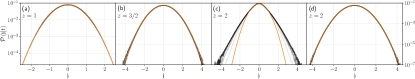
Figure 1: Convergence of distributions $\mathcal{P}(\mathfrak{j}|t)$ for various dynamical regimes: (a) integrable easy-plane regime with ballistic exponent $z=1$, (b) integrable isotropic model with superdiffusive exponent $z=3/2$ and (c) integrable easy-axis regime with diffusive exponent $z=2$. For comparison, (d) is a non-integrable isotropic trotterization with $z=2$. Best-fit Gaussian distributions are depicted by full orange lines. Time increases from gray $(t=40)$ to black $(t=500)$. Simulation parameters: timestep $\tau=1$, length $L=2^{10}$, anisotropy $\varrho=\gamma=1$, $N_{\textrm{avg}}=3\times 10^{5}$. The models and conventions are given in sup .

Strikingly, in the diffusive and superdiffusive dynamics regimes we encounter hitherto undisclosed anomalous fluctuations and divergent scaled cumulants.

Fluctuations on typical scale.— Our main objective is to characterize the dynamics of magnetization in a one-dimensional classical spin system governed by a deterministic equation of motion for the spin field ${\bf S}\equiv(S^{1},S^{2},S^{3})^{\rm T}$ (subject to constraint $|{\bf S}|=1$). We are specifically interested in extended (i.e. thermodynamic) homogeneous systems of interacting spins in which the third component of total magnetization is a globally conserved charge, $Q=\int{\rm d}x\,S^{3}(x)$, satisfying a local continuity equation $\partial_{t}S^{3}(x,t)+\partial_{x}j(x,t)=0$.

In this work, we aim to characterize the fluctuations of the time-integrated spin current density passing through the origin in a finite interval of length $t$,

$$\mathfrak{J}(t)=\int^{t}_{0}{\rm d}t^{\prime}\,j(0,t^{\prime}).$$ (1)

Equation (1) represents the net transferred magnetization between two semi-infinite regions of the system that can be regarded as a fluctuating macroscopic dynamical variable, and the main scope of this work is to examine its statistical properties in thermal equilibrium. While on average there is no transferred charge, $\langle\mathfrak{J}(t)\rangle=0$, the variance of $\mathfrak{J}(t)$ at large times times grows algebraically with an equilibrium dynamical exponent $z$,

$$\left\langle[\mathfrak{J}(t)]^{2}\right\rangle^{c}\sim t^{1/z},$$ (2)

where $\langle\bullet\rangle^{c}$ denotes the connected part of the $n$-point correlation in thermal equilibrium. For simplicity, we shall subsequently compute averages with respect to an unbiased stationary measure, representing the high-temperature limit of the canonical Gibbs ensemble.

Notice that typical fluctuations of $\mathfrak{J}(t)$ are of the order $\mathcal{O}(t^{1/2z})$. In order to quantify them, we introduce the dynamical distribution $\mathcal{P}(\mathfrak{j}|t)$ of the scaled integrated current density

$$\mathfrak{j}(t)\equiv t^{-1/2z}\mathfrak{J}(t),$$ (3)

and subsequently determine the stationary probability distribution that may emerge at large times, $\mathcal{P}(\mathfrak{j})=\lim_{t\to\infty}\mathcal{P}(\mathfrak{j}|t)$, normalized as $\int\mathcal{P}(\mathfrak{j}|t){\rm d}\mathfrak{j}=1$. We shall characterize it by its cumulants $\kappa_{n}=\lim_{t\to\infty}\kappa_{n}(t)$,

$$\kappa_{n}(t)\equiv\left\langle[\mathfrak{j}(t)]^{n}\right\rangle^{c}=t^{-n/2z}\left\langle[\mathfrak{J}(t)]^{n}\right\rangle^{c}.$$ (4)

By the time-reversal symmetry of an equilibrium state $\mathcal{P}(\mathfrak{j})$ is symmetric and hence $\kappa_{2n+1}=0$ for all $n\in\mathbb{N}$. If all $\kappa_{n\neq 2}=0$, then $\mathcal{P}(\mathfrak{j})$ takes the form of a Gaussian and typical fluctuations are said to be normal. For rapidly decaying temporal correlations of local currents, this property, for $z=1$, is indeed guaranteed by the central limit theorem, as eg. in rule 54 dynamics Buča et al. (2021). In Hamiltonian systems, temporal correlations of currents of conserved charges are invariably present and very little is known about their clustering properties, therefore no general conclusions about the dynamical exponent and Gaussianity of $\mathfrak{J}(t)$ can be drawn. However, in non-integrable (chaotic) systems having the hydrodynamic mode with zero velocity, one may expect spatiotemporal correlations to follow diffusive phenomenology, implying dynamical exponent $z=2$ and Gaussian fluctuations.

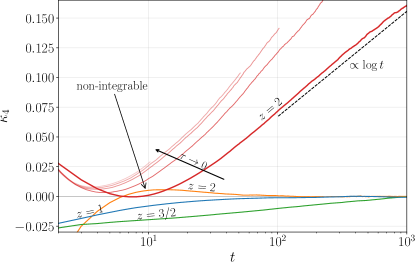
Figure 2: Time dependence of $\kappa_{4}(t)$ in different dynamical regimes characterized by the dynamical exponent $z$: diffusive easy-axis regime (red curves, indicating dependence on time-step $\tau\in\{1,0.3,0.1,0.05,0.01\}$), isotropic point (green), ballistic easy-plane regime (blue), and diffusive isotropic non-integrable model (orange). Dashed black line indicates a $\log t$ dependence as a guide to the eye. Other simulation parameters: timestep $\tau=1$, length $L=2^{11}$, anisotropy $\varrho=\gamma=1$, $N_{\rm avg}=3\times 10^{5}$. The models and conventions are given in sup .

Fluctuations in an integrable magnet.— We subsequently consider the anisotropic Landau–Lifshitz magnet, one of the best studied paradigms of interacting spins. In continuous space-time, the model is described by the equation of motion

$$\partial_{t}{\bf S}={\bf S}\times\partial^{2}_{x}{\bf S}+{\bf S}\times{\mathrm{J}}\,{\bf S},$$ (5)

with anisotropy tensor $\mathrm{J}={\rm diag}(0,0,\delta)$, representing one of the simplest completely integrable PDEs Takhtajan (1977); Faddeev and Takhtajan (1987). Equation (5) is particularly convenient since tuning the anisotropy $\delta$ permits the study of three distinct dynamical regimes Prosen and Žunkovič (2013); Krajnik and Prosen (2020); Krajnik et al. (2021): (i) the ‘easy-plane’ ballistic regime ($z=1$, $\delta<0$), (ii) the easy-axis diffusive regime ($z=2$, $\delta>0$) and finally (iii) the isotropic point with superdiffusive spin transport ($z=3/2$, $\delta=0$) – in exact correspondence with the dynamical phases of the Heisenberg $XXZ$ spin-$1/2$ chain Bulchandani et al. (2021). Indeed, Eq. (5) is known to be the effective evolution law for the semi-classical eigenstates (i.e. spin waves of large wavelengths) in the quantum spin chain (see e.g. De Nardis et al. (2020); Miao et al. (2021)).

We have performed numerical simulations on the lattice counterpart of Eq. (5) (details in sup ). One should be aware that a naïve lattice discretization of Eq. (5) does not preserve integrability, which may introduce certain spurious effects that affect dynamical properties at large times. This can be overcome by taking advantage of an exact symplectic integrator based on an integrable regularization in discrete space-time constructed in Ref. Krajnik et al. (2021), thereby significantly boosting efficiency of numerical integration (we have verified that the results do not qualitatively change upon varying the time-step $\tau$, see Fig. 2). The accuracy of our data is only subject to statistical errors due to the size $N_{\rm avg}$ of an ensemble of initial conditions sampling the unbiased equilibrium infinite temperature state.

We start by assessing the fluctuations of transferred magnetization $\mathfrak{J}(t)=\sum_{x>0}(S^{3}_{x}(t)-S^{3}_{x}(0))$ by computing the dynamical distribution of the integrated current $\mathcal{P}(\mathfrak{j}|t)$, rescaled to the timescale of typical fluctuations. There results are collected in Fig. 1. Most notably, we observe a significant deviation from Gaussianity in the diffusive case (Fig. 1c). In all other regimes of interest, fluctuations appear to be fairly consistent with a Gaussian profile. To quantify the degree of non-Gaussianity we focus next on the fourth cumulant $\kappa_{4}(t)$, see Fig. 2, where we observe (approximately) logarithmic divergence of $\kappa_{4}$ in the diffusive (i.e. easy-axis) regime, while in other cases $\kappa_{4}(t)$ converges to zero.

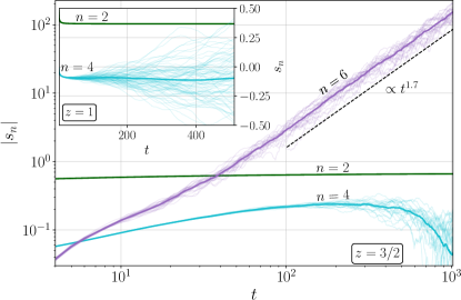
Figure 3: Temporal growth of scaled cumulants $s_{n}(t)$ (absolute values) at (main figure) the isotropic point ($z=3/2$) and (inset) in the easy plane regime ($z=1$). Faint lines show $N_{\rm par}$ partial averages, each over $N_{\rm avg}$ initial random spin configurations. Full line is the total average over $N_{\rm par}\cdot N_{\rm avg}$ initial configurations. Dashed black line indicates the scaling $s_{6}(t)\sim t^{\nu_{6}}$ with $\nu_{6}\approx 1.7$. Simulation parameters: timestep $\tau=1$, length $L=2^{11}\,(\textrm{main figure})$, $2^{10}\,(\textrm{inset})$, anisotropy $\gamma=1$ (inset), $N_{\rm avg}=3\times 10^{5}$, $N_{\rm par}=25\,(\textrm{main figure}),10^{2}\,(\textrm{inset})$. The models and conventions are given in sup .

Long-time growth of cumulants.— The discernible departure from Gaussianity indicates that spin transport in the diffusive phase escapes the usual paradigm of normal diffusion, as conventionally described within the framework of the MFT. In the scope of LD theory, another universal feature of stochastic diffusive systems (such as e.g. simple exclusion processes) is the existence of the scaled cumulants $s_{n}(t)=t^{-1/z}\left\langle[\mathfrak{J}(t)]^{n}\right\rangle^{c}=({\rm d}/{\rm d}\lambda)^{n}F(\lambda|t)|_{\lambda=0}$, where $F(\lambda|t)\equiv t^{-1/z}\log\left\langle e^{\lambda\mathfrak{J}(t)}\right\rangle$. Following the standard prescription form the literature, the limits of scaled cumulants can be computed from the series expansion of the scaled cumulant generating function (SCGF) $F(\lambda)=\lim_{\to\infty}F(\lambda|t)$ as $\lim_{t\to\infty}s_{n}(t)=({\rm d}/{\rm d}\lambda)^{n}F(\lambda)|_{\lambda=0}$. This scheme however hinges on certain subtle requirements Ž. Krajnik et al. which, as we argue next, may be violated in integrable deterministic dynamics. Specifically, we show in Fig. 3 that the scaled cumulants diverge in the isotropic and easy-axis regimes of our model, i.e. when $z>1$. At the isotropic point $\delta=0$ we detect a robust algebraic divergence of the sixth scaled cumulant $s_{6}(t)\sim t^{\nu_{6}}$ with $\nu_{6}\approx 1.7$, in turn implying divergent $\kappa_{6}(t)=t^{-4/(2z)}\,s_{6}(t)$. It is worth noting that such a ‘higher-order discrepancy’ of a tiny amplitude $\kappa_{6}\lessapprox 10^{-2}$ on the accessible timescale (by order of magnitude smaller than in the diffusive regime, cf. Figure 2) can hardly be discerned from Figure 1b), where no noticeable deviations from Gaussianity are visible. Lastly, in the easy-plane (i.e. ballistic) regime, the scaled cumulant $s_{4}(t)$ converges to a finite value, see inset in Fig. 4. Although a reliable extraction of higher scaled cumulants is obstructed by the rapidly growing spread of partial averages, our data (see sup ) gives no indications of divergent scaled cumulants. We finally note that upon (strongly) breaking integrability, scaled cumulants are expectedly finite for any value of anisotropy (see sup ).

Fluctuations out of equilibrium.—A convenient setting that is widely used for studying fluctuations of charge transfer in one-dimensional systems away from equilibrium is the two-partition protocol. Several important analytic results have been obtained in this way, predominantly in the domain of stochastic systems Johansson (2000); Tracy and Widom (2009a, b); Eisler and Rácz (2013); Bulchandani and Karrasch (2019); Derrida and Gerschenfeld (2009). To study fluctuations of transferred magnetization, one initializes the system in two semi-infinite partitions in equilibrium states at equal temperatures and opposite chemical potentials $\pm\mu$, related to magnetization densities via $\langle S^{3}\rangle(\mu)=\coth{(\mu)}-\mu^{-1}$. The ensuing dynamical interface region expands asymptotically as $x\sim t^{1/\varkappa}$ while reaching a ‘local quasi-stationary state’. Owing to a finite bias (i.e. a jump in the chemical potential $\mu$), the average integrated current does not vanish and (by assuming algebraic asymptotic scaling) we can accordingly write $\langle\mathfrak{J}(t)\rangle_{\rm noneq}\sim t^{1/\varkappa}$.

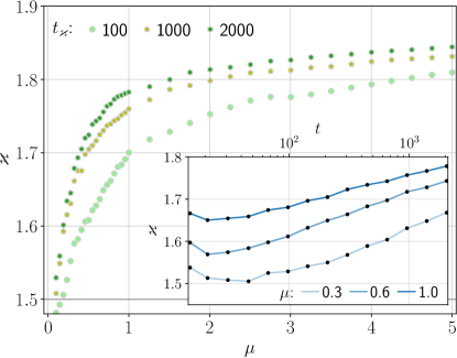
Figure 4: Estimated dynamical exponent $\varkappa$ depending on chemical potential $\mu$ for different integration times $t_{\varkappa}$ (with gray line showing $z_{\rm KPZ}=3/2$). (inset) Time dependnece of the estimated exponent for $\mu\in\{0.3,0.6,1.0\}$. Simulation parameters: $\tau=1$, $L=2^{12}$, $N_{\rm avg}=$ $3\times 10^{5}$ (main figure), $10^{6}$ (inset). The models and conventions are given in sup .

Regarding a practical implementation there are now two major stumbling blocks that one has to confront: (I) our simulations reveal (see Fig. 4) that the running (i.e. time-dependent) algebraic exponent $\varkappa$ converges very slowly towards the expected value at late times, thereby preventing reliable estimation of the stationary distribution $\mathcal{P}(\mathfrak{j})$ of the rescaled current; (II) due to absence of translational symmetry in the initial state, the sampling size is reduced by a factor of system length $L$ compared to the equilibrium setting. It is nonetheless instructive to expand on point (I). Firstly, we wish to point out that the nonequlibrium dynamical exponent $\varkappa$ should not be a-priori identified with the equilibrium exponent $z$ that governs the asymptotic growth of the variance (see Eq. (2)). As we shortly demonstrate, this is delicate matter at the isotropic point ($\delta=0$) where the equilibrium dynamical exponent $z_{\rm KPZ}=3/2$ of the Kardar–Parisi–Zhang (KPZ) equation Kardar et al. (1986) is known to be ‘protected’ by a global nonabelian symmetry Krajnik et al. (2020a); Bulchandani et al. (2021) that has to be preserved both at the level of the time propagator and the underlying equilibrium state. Despite the fate of KPZ scaling becomes less obvious upon departing from equilibrium, a recent experimental study suggests that it might survive Wei et al. (2021).

Implementing a two-partition protocol, we numerically extract the running dynamical exponent $\varkappa$ as a function of $\mu$ as shown in Fig. 4. For any finite simulation time $t_{\varkappa}$, we observe a smooth crossover from $\varkappa\approx 3/2$ in the vicinity of $\mu\to 0$ towards the diffusive exponent $\varkappa\approx 2$ upon approaching strong polarizations $\mu\to\infty$. This indicates that in spite of a pronounced $\mu$-dependent transient, the running dynamical exponent eventually saturates to $\varkappa=2$. This analysis is aligned with theoretical expectation: KPZ physics of spin transport is sensitive to explicit breaking of rotational symmetry (here by the initial nonequilibrium state); our simulations show that the broken symmetry is not dynamically restored, and the dynamics is more reminiscent of the melting magnetic domain at zero temperature Gamayun et al. (2019); Misguich et al. (2019).

Conclusion.—We numerically investigated the properties of fluctuations in various dynamical regimes of the one-dimensional lattice Landau–Lifshitz magnet by computing the distribution of the time-integrated spin current and analyzing the time dependence of its cumulants. Most strikingly, we encountered non-Gaussian typical fluctuations on sub-ballistic scales, comprising both the diffusive easy-axis regime and the isotropic point with superdiffusive spin transport (where the effect is much less pronounced). This follows as a consequence of divergent scaled cumulants, which moreover imply that the SCGF is not a generator of scaled cumulants. While two-point functions in the easy-axis ($\mathbb{Z}_{2}$-symmetric) and isotropic (SU(2)-symmetric) regimes have previously been found to excellently match Ljubotina et al. (2017, 2019); Weiner et al. (2020); Krajnik and Prosen (2020); Krajnik et al. (2021), respectively, the diffusive (Gaussian) and KPZ (Prähoffer-Spohn Prähofer and Spohn (2004)) scaling functions, our new data shows that higher-point functions (or distribution of fluctuations) are distinct from diffusive and KPZ universality classes. In particular, as KPZ equation manifestly refers to out-of-equilibrium, breaking detailed balance, the distribution of finite time fluctuations in the KPZ equation are always skewed (eg. Tracy-Widom or Baik-Rains, depending on the initial condition) unlike in our equilibrium scenario, where they are symmetric.

On the ballistic timescale, i.e. at finite magnetization density or in the easy-plane regime at zero magnetization, we found no traces of irregular or non-normal behavior (apart from considerably slower convergence of averages compared to a nonintegrable chain). By explicitly breaking integrability we restored ergodicity and we expectedly recovered both the Gaussian form of typical fluctuations and finite scaled cumulants. This suggests that the observed singularity of the SCGF is subtly linked to the presence of interacting quasiparticles (solitons, see Ref. Faddeev and Takhtajan (1987); Ablowitz and Segur (1981), whose asymptototic stability is ensured by a hierarchy of non-trivial conservation laws) which we envision to be responsible for ‘weak’ clustering of temporal multipoint current correlations. This possibility has been discussed in Ref. Doyon and Myers (2019), where it is argued that anomalous fluctuations could occur on the ballistic scale along the ray corresponding to an isolated co-propagating normal mode. As per Doyon and Myers (2019) however, a continuous spectrum of normal modes (which is to be anticipated in the Landau–Lifshitz magnet, by analogy to the quantum Heisenberg chain) need not necessarily be detrimental for Gaussianity. Concerning the ballistic regime, the absence of any irregularities is thus consistent with the described scenario. Altough the exact expressions for low-order cumulants have been recently derived Perfetto and Doyon (2021) by employing the ‘generalized hydrodynamics’ Castro-Alvaredo et al. (2016); Bertini et al. (2016), their explicit evaluation crucially relies on the knowledge of the ‘flux Jacobian’ Doyon (2020) which for the particular case of the anisotropic Landau–Lifshitz model is currently out of reach. The discernible divergence of scaled cumulants that we captured on subballistic scales however goes beyond the current capabilities and for the time being remains entirely elusive. In this view, the most pressing question is to identify a microscopic mechanism responsible for the observed anomalous behavior.

Our hope is that the technical difficulties we encountered in extending our analysis to the nonequilibrium setting can be surmounted, as it would help tremendously to establish a more complete phenomenological picture. It would likewise be valuable to complement the earlier findings of Ref. Žnidarič (2014c) by a similar analysis for the case of the anisotropic quantum Heisenberg chain. Our expectation here is that the anomalous structure of dynamical fluctuations in subballistic regimes will also surface at the quantum level. Finally, amidst many recent experimental breakthroughs we firmly believe the time is ripe to initiate a pursuit to find irregular features in flucuating macroscopic quantities.

Acknowledgements.

We thank I. Bloch, S. Gopalakrishnan, V. Pasquier, V. Popkov, J. Schmidt, J. Zeiher and M. Žnidarič for insightful discussions and comments. ŽK acknowledges support of the Milan Lenarčič foundation. This work has been supported by the European Research Council (ERC) under the Advanced Grant No. 694544 – OMNES, and by the Slovenian Research Agency (ARRS) under the Program P1-0402.

Supplemental Material for
“Absence of Normal Fluctuations in an Integrable Magnet”

I Integrable discretizations

In this section, we collect the essential information about the integrable models used in our study. We employ an integrable space-time discretization of the classical Landau–Lifshitz one-dimensional magnet, whose continuum theory describe the motion of the classical spin field ${\bf S}=(S^{1},S^{2},S^{3})$ constrained to a two-sphere ${\bf S}\in\mathcal{S}\cong S^{2}$, evolving according to

$$\partial_{t}{\bf S}={\bf S}\times\partial^{2}_{x}{\bf S}+{\bf S}\times{\mathrm{J}}\,{\bf S},\qquad{\rm J}=\textrm{diag}(0,0,\delta),$$ (6)

where parameter $\delta\in\mathbb{R}$ parametrizes the interaction anisotropy. Using the $SO(3)$ Lie-Poisson algebra

$$\left\{S^{a}(x),S^{b}(y)\right\}=\sum_{c}\varepsilon^{abc}S^{c}(x)\delta(x-y),$$ (7)

where $\varepsilon$ is the Levi-Civita tensor, equation (6) can be cast in Hamiltonian form

$$\partial_{t}{\bf S}=\{{\bf S},H\}=-{\bf S}\times\frac{\delta H}{\delta{\bf S}},$$ (8)

with

$$H=\frac{1}{2}\int\left[\left(\partial_{x}{\bf S}\right)^{2}-{\bf S}\cdot{\rm J}{\bf S}\right]\,{\rm d}x.$$ (9)

Depending on the value of $\delta$, we distiguish between three different dynamical regimes characterized by the dynamical exponent $z$ (in a maximum entropy state with no net magnetization, see Eq. (2) of the main text):

$$\delta \,>0\quad\textrm{easy-axis regime, } z=2,$$

$$\delta \,=0\quad\textrm{isotropic regime, } z=3/2,$$

$$\delta \,>0\quad\textrm{easy-plane regime, } z=1.$$ (10)

I.1 Space-time discretization

We briefly review an integrable space-time lattice discretization of Eq. (6) constructed in Refs. Krajnik and Prosen (2020); Krajnik et al. (2020a). The main object of the integration scheme is a two-body map $\Phi_{\tau}:\mathcal{S}\times\mathcal{S}\mapsto\mathcal{S}\times\mathcal{S}$ that provides a local propagator for a pair of adjacent spins

$$({\bf S}_{1},{\bf S}_{2})\mapsto({\bf S}_{1}^{\prime},{\bf S}_{2}^{\prime}).$$ (11)

The parameter $\tau\in\mathbb{R}_{+}$ is an ajustable integration timestep. The two-body propagator (11) serves as the elementary building block of the full (i.e. many-body) propagator $\Phi^{\textrm{full}}:\mathcal{S}^{\times L}\mapsto\mathcal{S}^{\times L}$ over the phase space of $L$ spins (where $L\in 2\mathbb{N}$), consisting of alternating odd and even steps (see Fig. 5)

$$(\vec{S}^{2t+2}_{2\ell-1},\vec{S}^{2t+2}_{2\ell})=\Phi(\vec{S}^{2t+1}_{2\ell-1},\vec{S}^{2t+1}_{2\ell}),\qquad(\vec{S}^{2t+1}_{2\ell},\vec{S}^{2t+1}_{2\ell+1})=\Phi(\vec{S}^{2t}_{2\ell},\vec{S}^{2t}_{2\ell+1}).$$ (12)

By making use of the embedding prescription, $\Phi^{(j)}=I^{\times(j-1)}\,\times\,\Phi_{\tau}\,\times\,I^{\times(L-j-1)}$, the full propagator $\Phi^{\rm full}$ for two units of time $t\mapsto t+2$ decomposes as

$$\Phi^{{\rm full}}=\Phi^{\rm even}\circ\Phi^{\rm odd},$$ (13)

with odd and even propagators further factorizing into commuting two-body maps,

$$\Phi^{\rm odd}=\prod_{\ell=1}^{L/2}\Phi^{(2\ell)},\qquad\Phi^{\rm even}=\prod_{\ell=1}^{L/2}\Phi^{(2\ell-1)}.$$ (14)

Such an integration scheme constitutes an integrable Trotterization of Eq. (6).

Figure 5: Symplectic circuit from two-body propagators: classical spin degrees of freedom $\vec{S}^{t}_{\ell}$ (circles) are attach to the middle of the edges of a discrete space-time lattice represented by a tilted checkerboard. A two-body symplectic map $\Phi_{\tau}$ (red square) that maps a pairs of incoming physical spins forward in time is attached to the middle of each square plaquette. [The figure has been reproduced from Ref. Krajnik et al. (2021).]

I.2 Integrable two-body propagators

I.2.1 Isotropic interaction

The integrable two-body propagator for the isotropic interaction was obtained in Ref. Krajnik and Prosen (2020)

$$\Phi_{\tau}(\vec{S}_{1},\vec{S}_{2})=\frac{1}{s^{2}+\tau^{2}}\left(s^{2}\mathbf{S}_{1}+\tau^{2}\vec{S}_{2}+\tau\vec{S}_{1}\times\vec{S}_{2},s^{2}\vec{S}_{2}+\tau^{2}\vec{S}_{1}+\tau\vec{S}_{2}\times\vec{S}_{1}\right),\quad s^{2}=\frac{1}{2}\left(1+\vec{S}_{1}\cdot\vec{S}_{2}\right),$$ (15)

and manifestly preserves the total spin

$$\vec{S}_{1}+\vec{S}_{2}=\vec{S}_{1}^{\prime}+\vec{S}_{2}^{\prime}.$$ (16)

I.2.2 Anisotropic interaction

The integrable space-time discretization in the anisotropic case was obtained in Ref. Krajnik et al. (2021), which can be compactly expressed in terms of ‘Sklyanin’ variables $\mathcal{K},\,\mathcal{S}^{\pm}$, satisfying the following Poisson relations,

$$\{\mathcal{K},\mathcal{S}^{\pm}\}=\mp{\rm i}\varrho\,\mathcal{S}^{\pm}\mathcal{K},\qquad\{\mathcal{S}^{+},\mathcal{S}^{-}\}=-\frac{{\rm i}\varrho}{2}\left(\mathcal{K}^{2}-\mathcal{K}^{-2}\right),$$ (17)

with the Casimir function $\mathcal{C}_{0}\equiv\mathcal{S}^{+}\mathcal{S}^{-}+\tfrac{1}{4}\left(\mathcal{K}-\mathcal{K}^{-1}\right)^{2}$. The two-body propagator takes the form

$$\left(\frac{\mathcal{K}^{\prime}_{1}}{\mathcal{K}_{1}}\right)^{2} =\frac{(\nu^{2}+\nu^{-2})\left(\mathcal{K}_{1}\mathcal{K}_{2}+\mathcal{K}_{1}^{-1}\mathcal{K}_{2}^{-1}\right)-2\mathcal{K}_{1}\mathcal{K}_{2}^{-1}-(w^{2}+w^{-2})\mathcal{K}_{1}^{-1}\mathcal{K}_{2}+4w\mathcal{S}^{+}_{1}\mathcal{S}^{-}_{2}+4w^{-1}\mathcal{S}^{-}_{1}\mathcal{S}^{+}_{2}}{(\nu^{2}+\nu^{-2})\left(\mathcal{K}_{1}\mathcal{K}_{2}+\mathcal{K}_{1}^{-1}\mathcal{K}_{2}^{-1}\right)-2\mathcal{K}_{1}^{-1}\mathcal{K}_{2}-(w^{2}+w^{-2})\mathcal{K}_{1}\mathcal{K}_{2}^{-1}+4w\mathcal{S}^{-}_{1}\mathcal{S}^{+}_{2}+4w^{-1}\mathcal{S}^{+}_{1}\mathcal{S}^{-}_{2}},$$

$$\left(\frac{\mathcal{K}^{\prime}_{2}}{\mathcal{K}_{2}}\right)^{2} =\frac{(\nu^{2}+\nu^{-2})\left(\mathcal{K}_{1}\mathcal{K}_{2}+\mathcal{K}_{1}^{-1}\mathcal{K}_{2}^{-1}\right)-2\mathcal{K}_{1}^{-1}\mathcal{K}_{2}-(w^{2}+w^{-2})\mathcal{K}_{1}\mathcal{K}_{2}^{-1}+4w\mathcal{S}^{-}_{1}\mathcal{S}^{+}_{2}+4w^{-1}\mathcal{S}^{+}_{1}\mathcal{S}^{-}_{2}}{(\nu^{2}+\nu^{-2})\left(\mathcal{K}_{1}\mathcal{K}_{2}+\mathcal{K}_{1}^{-1}\mathcal{K}_{2}^{-1}\right)-2\mathcal{K}_{1}\mathcal{K}_{2}^{-1}-(w^{2}+w^{-2})\mathcal{K}_{1}^{-1}\mathcal{K}_{2}+4w\mathcal{S}^{+}_{1}\mathcal{S}^{-}_{2}+4w^{-1}\mathcal{S}^{-}_{1}\mathcal{S}^{+}_{2}},$$

$$\begin{bmatrix}(\mathcal{S}^{\pm}_{1})^{\prime}\\ (\mathcal{S}^{\pm}_{2})^{\prime}\end{bmatrix} =\Omega(w^{\pm 1})\begin{bmatrix}\mathcal{S}^{\pm}_{1}\\ \mathcal{S}^{\pm}_{2}\end{bmatrix},$$ (18)

with

$$\Omega(w)=\frac{1}{\mathcal{K}_{1}\mathcal{K}_{2}w-(\mathcal{K}_{1}\mathcal{K}_{2}w)^{-1}}\!\begin{bmatrix}\mathcal{K}^{\prime}_{1}\mathcal{K}_{2}-(\mathcal{K}^{\prime}_{1}\mathcal{K}_{2})^{-1}&\kern-10.00002pt(\mathcal{K}^{\prime}_{1}/\mathcal{K}_{1})w-(\mathcal{K}_{1}/\mathcal{K}^{\prime}_{1})w^{-1}\\ (\mathcal{K}^{\prime}_{2}/\mathcal{K}_{2})w-(\mathcal{K}_{2}/\mathcal{K}^{\prime}_{2})w^{-1}&\kern-10.00002pt\mathcal{K}^{\prime}_{1}\mathcal{K}_{2}-(\mathcal{K}^{\prime}_{1}\mathcal{K}_{2})^{-1}\end{bmatrix},$$ (19)

and parameters

$$\nu=e^{\varrho},\qquad w=e^{{\rm i}\varrho\tau}.$$ (20)

The anisotropy of interaction is controlled by a parameter $\varrho$ with the following domains:

– $$\textrm{ the \emph{easy-axis} regime with anisotropy }\varrho\in\mathbb{R}_{+},$$

– $$\textrm{ the \emph{easy-plane} regime with anisotropy }\gamma\in[-\pi/2,\pi/2].$$ (21)

The easy plane anisotropy $\gamma$ is related to the easy axis anisotropy via analytic continuation as $\varrho\to{\rm i}\gamma$. Sklyanin’s spins are bijectively related to classical spins via

$$\mathcal{K}=e^{\varrho\,S^{3}},\qquad\mathcal{S}^{\pm}=F_{\varrho}(S^{3})S^{\pm},\quad F_{\varrho}(s)\equiv\sqrt{\frac{\sinh^{2}(\varrho)-\sinh^{2}(\varrho s)}{1-s^{2}}}.$$ (22)

The propagator (18) preserves the third component of magnetization

$$S^{3}_{1}+S^{3}_{2}=(S^{3}_{1})^{\prime}+(S^{3}_{2})^{\prime}.$$ (23)

I.3 Discrete Noether current

The full propagator has a global $U(1)$ symmetry which implies a conserved charge $Q=\sum_{\ell}q_{\ell}$, representing the total magnetization along the third axis, $q_{\ell}=S^{3}_{\ell}$. Due to the even-odd structure of the dynamics, Eq. (13), the local density satisfies a pair of discrete continuity equations

$$\frac{1}{\tau}\left(q_{2\ell}^{2t+2}-q_{2\ell}^{2t}\right)+j_{2\ell+1}^{2t+1}-j_{2\ell}^{2t}=0,\qquad\frac{1}{\tau}\left(q_{2\ell+1}^{2t+2}-q_{2\ell+1}^{2t}\right)+j_{2\ell+2}^{2t}-j_{2\ell+1}^{2t+1}=0,$$ (24)

which are satisfied by a current of the form

$$j_{\ell}^{t}\equiv j(\ell,t)=\frac{1}{\tau}\big{(}q_{\ell}^{t+1}-q_{\ell}^{t}\big{)}.$$ (25)

I.4 Ensemble average

We introduce the stationary maximum entropy measure $\rho_{1}$ on $\mathcal{S}$ (i.e. Gibbs states at infinite temperature) and define a separable measure $\rho_{L}$ by extending it to the many-body phase $\mathcal{M}_{L}\equiv\mathcal{S}^{\times L}$, namely

$$\rho_{L}=\prod_{\ell=1}^{L}\rho_{1}(\vec{S}_{\ell}).$$ (26)

For the normalized one-body measure we consider the grand-canonical ensemble with a chemical potential $\mu\in\mathbb{R}$,

$$\rho_{1}(\vec{S})=\frac{1}{4\pi}\frac{\mu}{\sinh\mu}e^{\mu\,S^{3}}.$$ (27)

Passing to the thermodynamic limit by sending $L\to\infty$, the grand-canonical partition function per site is given by

$$\mathcal{Z}_{1}(\mu)=\int_{\mathcal{S}}{\rm d}\Omega\,\rho_{1}(\vec{S})=\frac{4\pi\sinh{\mu}}{\mu},$$ (28)

with ${\rm d}\Omega$ denoting the volume element on $\mathcal{S}$. Writting ${\rm d}\Omega^{\rm full}\equiv\prod_{\ell=1}^{L}{\rm d}\Omega(\vec{S}_{\ell})$, the average of a local observable $\mathcal{O}$ is computed as

$$\langle\mathcal{O}\rangle_{\mu}=\lim_{L\to\infty}\big{[}\mathcal{Z}^{L}_{1}(\mu)\big{]}^{-1}\int_{\mathcal{M}_{L}}{\rm d}\Omega^{\rm full}\,\rho_{L}\,\mathcal{O}.$$ (29)

The average magnetization is related to $\mu$ via

$$\langle S^{3}\rangle(\mu)=\coth{\mu}-1/\mu.$$ (30)

I.5 Field theory limit

The reduction to the field theory involves two steps. Firstly, we send $\tau\to 0$ to obtain a Hamiltonian lattice model

$$H_{\rm LLL}^{\varrho}\simeq\sum_{\ell=1}^{L}\log\left[(\sinh\varrho)^{2}\,\mathcal{S}^{0}_{\ell}\mathcal{S}^{0}_{\ell+1}+\mathcal{S}^{1}_{\ell}\mathcal{S}^{1}_{\ell+1}+\mathcal{S}^{2}_{\ell}\mathcal{S}^{2}_{\ell+1}+(\cosh\varrho)^{2}\,\mathcal{S}^{3}_{\ell}\mathcal{S}^{3}_{\ell+1}\right],$$ (31)

in terms of Sklyanin spins $\mathcal{S}^{0}\equiv\frac{1}{2}(\mathcal{K}+\mathcal{K}^{-1}),\enspace\mathcal{S}^{1}\equiv\frac{1}{2}(\mathcal{S}^{+}+\mathcal{S}^{-}),\enspace\mathcal{S}^{2}\equiv\frac{1}{2{\rm i}}(\mathcal{S}^{+}-\mathcal{S}^{-}),\enspace\mathcal{S}^{3}\equiv\frac{1}{2}(\mathcal{K}-\mathcal{K}^{-1}).$ We then reinstate a lattice spacing $\varDelta$ and subsequently retain smooth lattice spin configurations $\vec{S}_{\ell}=\vec{S}(x=\Delta\ell)$, $\vec{S}_{\ell\pm 1}=\vec{S}(x)\pm\varDelta\partial_{x}\vec{S}+\frac{1}{2}\varDelta^{2}\,\partial_{x}^{2}\vec{S}+\mathcal{O}(\varDelta^{3})$ by keeping only variations at the leading non-trivial order $\mathcal{O}(\varDelta^{2})$. Finally taking the continuum limit $\varDelta\to 0$, both the Sklyanin variables and the anisotropy parameter have to be rescaled by the lattice spacing, namely

$$\mathcal{S}^{0}=1+\mathcal{O}(\varDelta^{2}),\qquad\mathcal{S}^{a}=\varDelta\,\vec{S}^{a}+\mathcal{O}(\varDelta^{2})\quad{\rm for}\quad a=1,2,3,$$ (32)

and $\varrho\rightarrow\varDelta\,\varrho$, thus recovering the Hamiltonian of the Landau–Lifshitz field theory,

$$H=\frac{1}{2}\int\left[\left(\partial_{x}{\bf S}\right)^{2}-{\bf S}\cdot{\rm J}{\bf S}\right]\,{\rm d}x,\qquad{\rm J}=\textrm{diag}(0,0,\varrho^{2}),$$ (33)

upon making the identification $\delta=\varrho^{2}$.

I.6 Integrable easy-plane regime: higher scaled cumulants

Here we provide the numerical data on scaled higher cumulants $s_{n}(t)$ associated to the time-integrated current density (refer to the main text for definitions) in the ballistic ($z=1$) easy-plane regime of (18). The non-zero scaled cumulants $n=6$ and $n=8$ are shown in Fig. 6. The rapidly growing spread of partial averages makes it difficult to make any definite statements about the asymptotic values of $s_{n\geq 6}(t)$. We nevertheless observe no significant divergent behaviour in any of the cumulants and attribute the late-time behaviour of $s_{6}(t)$ and $s_{8}(t)$ to statistical fluctuations (thin lines) which are an order of magnitude larger than the magnitude of the average (thick line). We emphasize that the full average is not the arithmetic average of partial averages owing to the nonlinearity of the cumulants.

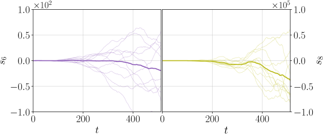
Figure 6: Temporal growth of scaled cumulants $s_{6},s_{8}$ in the easy-plane regime ($z=1$). Faint lines show $N_{\rm par}$ partial averages, each over $N_{\rm avg}$ initial random spin configurations. Full line is the total average over $N_{\rm par}\cdot N_{\rm avg}$ initial configurations. Simulation parameters: timestep $\tau=1$, length $L=2^{10}$, anisotropy $\gamma=1$, $N_{\rm avg}=6\times 10^{6}$, $N_{\rm par}=10$.

II Non-integrable discretizations

It is instructive to make a comparisson to an ergodic Hamiltonian dynamics. To this end, we also consider the scaled cumulants of the time integrated current density in nonintegrable discretizations of the anisotropic Landau-Lifhsitz field theory, Eq. (6), as outlined below.

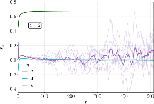
Figure 7: Temporal growth of scaled cumulants $s_{n}$ in the nonintegrable isotropic regime (z=2). Faint lines show $N_{\rm par}$ partial averages, each over $N_{\rm avg}$ initial random spin configurations. Full line is the total average over $N_{\rm par}\cdot N_{\rm avg}$ initial configurations. Simulation parameters: timestep $\tau=1$, length $L=2^{10}$, $N_{\rm avg}=3\times 10^{6}$, $N_{\rm par}=6$.

II.1 Two-body propagator for isotropic interaction

The isotropic dynamics can be efficiently discretized by employing the same Trotterization scheme (cf. Eq. (12)) as in the integrable case, only replacing the two-body propagator $\Phi_{\tau}$. Deriving an non-integrable two-body map is straighforward and does not require any integrability techniques. Instead, it suffices to find the explicit solution to the two-body problem governed by the simple Hamiltonian

$$H=\vec{S}_{1}\cdot\vec{S}_{2},$$ (34)

yielding the equations of motion (see also the Supplemental Material of Ref. Krajnik et al. (2020b))

$$\dot{\vec{S}}_{1}=\vec{S}_{1}\times\vec{S}_{2},\qquad\dot{\vec{S}}_{2}=\vec{S}_{2}\times\vec{S}_{1}.$$ (35)

A non-integrable two-body propagator $\Phi_{\tau}$ corresponds to evaluating the solution of the above at time $t=\tau$, yielding

$$S_{\ell}^{\prime}=e^{{\rm i}\tau S}S_{\ell}e^{-{\rm i}\tau S},\qquad{\rm with}\quad S=S_{1}+S_{2},\quad S_{\ell}=\vec{S}_{\ell}\cdot\boldsymbol{\sigma},\quad\ell=1,2,$$ (36)

where $\boldsymbol{\sigma}=(\sigma^{1},\sigma^{2},\sigma^{3})$ is a vector of Pauli matrices. The discrete dynamics given by Eq. (36) permits efficient simulation of non-integrable spin dynamics with local isotropic spin interaction.

II.2 Scaled cumulants

Simulating the non-integrable isotropic model, cf. Eq. (36), we expectedly observe diffusive spreading at late time, characterized by dynamical exponent $z=2$. We moreover computed the scaled cumulants $s_{n}(t)$ (shown in Fig. 7). We find that $s_{4}$ rapidly decays towards zero. The large spread of partial averages of $s_{6}(t)$ does not allow for an extraction of its asymptotic value, but we observe no systematic divergent behaviour (cf. Fig. 3 of the main text), indicating the existence of scaled cumulants in the nonintegrable model (36). Moreover $s_{6}$ asyptoticaly decaying towards zero is within the range of statistical fluctuations of the data.

References

- Cassidy et al. (2011) A. C. Cassidy, C. W. Clark, and M. Rigol, Physical Review Letters 106 (2011), 10.1103/physrevlett.106.140405.
- Vidmar and Rigol (2016) L. Vidmar and M. Rigol, Journal of Statistical Mechanics: Theory and Experiment 2016, 064007 (2016).
- Essler and Fagotti (2016) F. H. L. Essler and M. Fagotti, J. Stat. Mech. Theory Exp 2016, 064002 (2016).
- Caux (2016) J.-S. Caux, Journal of Statistical Mechanics: Theory and Experiment 2016, 064006 (2016).
- Ilievski et al. (2015) E. Ilievski, J. De Nardis, B. Wouters, J.-S. Caux, F. H. L. Essler, and T. Prosen, Phys. Rev. Lett. 115, 157201 (2015).
- Ilievski et al. (2016) E. Ilievski, M. Medenjak, T. Prosen, and L. Zadnik, Journal of Statistical Mechanics: Theory and Experiment 2016, 064008 (2016).
- Bertini et al. (2021) B. Bertini, F. Heidrich-Meisner, C. Karrasch, T. Prosen, R. Steinigeweg, and M. Žnidarič, Reviews of Modern Physics 93 (2021), 10.1103/revmodphys.93.025003.
- De Nardis et al. (2021) J. De Nardis, B. Doyon, M. Medenjak, and M. Panfil, arXiv preprint arXiv:2104.04462 (2021).
- Bulchandani et al. (2021) V. B. Bulchandani, S. Gopalakrishnan, and E. Ilievski, Journal of Statistical Mechanics: Theory and Experiment 2021, 084001 (2021).
- Alba and Calabrese (2018) V. Alba and P. Calabrese, SciPost Physics 4 (2018), 10.21468/scipostphys.4.3.017.
- Calabrese (2020) P. Calabrese, SciPost Physics Lecture Notes (2020), 10.21468/scipostphyslectnotes.20.
- De Nardis et al. (2018) J. De Nardis, D. Bernard, and B. Doyon, Physical Review Letters 121 (2018), 10.1103/physrevlett.121.160603.
- Gopalakrishnan et al. (2018) S. Gopalakrishnan, D. A. Huse, V. Khemani, and R. Vasseur, Physical Review B 98 (2018), 10.1103/physrevb.98.220303.
- Doyon et al. (2018) B. Doyon, T. Yoshimura, and J.-S. Caux, Phys. Rev. Lett. 120, 045301 (2018).
- Doyon et al. (2017) B. Doyon, J. Dubail, R. Konik, and T. Yoshimura, Phys. Rev. Lett. 119, 195301 (2017).
- Bastianello et al. (2019) A. Bastianello, V. Alba, and J.-S. Caux, Physical Review Letters 123 (2019), 10.1103/physrevlett.123.130602.
- Castella et al. (1995) H. Castella, X. Zotos, and P. Prelovšek, Physical Review Letters 74, 972 (1995).
- Zotos (1999) X. Zotos, Physical Review Letters 82, 1764 (1999).
- Prosen (2011) T. Prosen, Physical Review Letters 106 (2011), 10.1103/physrevlett.106.217206.
- Ilievski and De Nardis (2017a) E. Ilievski and J. De Nardis, Physical Review Letters 119 (2017a), 10.1103/physrevlett.119.020602.
- Doyon and Spohn (2017) B. Doyon and H. Spohn, SciPost Phys. 3, 039 (2017).
- Ilievski and De Nardis (2017b) E. Ilievski and J. De Nardis, Phys. Rev. B 96, 081118 (2017b).
- Žnidarič (2011) M. Žnidarič, Physical Review Letters 106 (2011), 10.1103/physrevlett.106.220601.
- Prosen and Žunkovič (2013) T. Prosen and B. Žunkovič, Physical Review Letters 111 (2013), 10.1103/physrevlett.111.040602.
- Ljubotina et al. (2017) M. Ljubotina, M. Žnidarič, and T. Prosen, Nature Communications 8 (2017), 10.1038/ncomms16117.
- Ilievski et al. (2018) E. Ilievski, J. De Nardis, M. Medenjak, and T. Prosen, Physical Review Letters 121 (2018), 10.1103/physrevlett.121.230602.
- Ljubotina et al. (2019) M. Ljubotina, M. Žnidarič, and T. Prosen, Physical Review Letters 122 (2019), 10.1103/physrevlett.122.210602.
- Gopalakrishnan and Vasseur (2019) S. Gopalakrishnan and R. Vasseur, Physical Review Letters 122 (2019), 10.1103/physrevlett.122.127202.
- De Nardis et al. (2019) J. De Nardis, M. Medenjak, C. Karrasch, and E. Ilievski, Physical Review Letters 123 (2019), 10.1103/physrevlett.123.186601.
- Dupont and Moore (2020) M. Dupont and J. E. Moore, Physical Review B 101 (2020), 10.1103/physrevb.101.121106.
- Bulchandani (2020) V. B. Bulchandani, Physical Review B 101 (2020), 10.1103/physrevb.101.041411.
- Ilievski et al. (2021) E. Ilievski, J. D. Nardis, S. Gopalakrishnan, R. Vasseur, and B. Ware, Physical Review X 11 (2021), 10.1103/physrevx.11.031023.
- Das et al. (2019) A. Das, M. Kulkarni, H. Spohn, and A. Dhar, Phys. Rev. E 100, 042116 (2019).
- Krajnik and Prosen (2020) Ž. Krajnik and T. Prosen, Journal of Statistical Physics 179, 110 (2020).
- Krajnik et al. (2020a) Ž. Krajnik, E. Ilievski, and T. Prosen, SciPost Phys. 9, 38 (2020a).
- Langen (2015) T. Langen, in Springer Theses (Springer International Publishing, 2015) pp. 111–121.
- Schemmer et al. (2019) M. Schemmer, I. Bouchoule, B. Doyon, and J. Dubail, Physical Review Letters 122 (2019), 10.1103/physrevlett.122.090601.
- Weiner et al. (2020) F. Weiner, P. Schmitteckert, S. Bera, and F. Evers, Physical Review B 101 (2020), 10.1103/physrevb.101.045115.
- Jepsen et al. (2020) P. N. Jepsen, J. Amato-Grill, I. Dimitrova, W. W. Ho, E. Demler, and W. Ketterle, Nature 588, 403 (2020).
- Malvania et al. (2021) N. Malvania, Y. Zhang, Y. Le, J. Dubail, M. Rigol, and D. S. Weiss, Science 373, 1129 (2021).
- Scheie et al. (2021) A. Scheie, N. E. Sherman, M. Dupont, S. E. Nagler, M. B. Stone, G. E. Granroth, J. E. Moore, and D. A. Tennant, Nature Physics 17, 726 (2021).
- Joshi et al. (2021) M. Joshi, F. Kranzl, A. Schuckert, I. Lovas, C. Maier, R. Blatt, M. Knap, and C. Roos, arXiv preprint arXiv:2107.00033 (2021).
- Wei et al. (2021) D. Wei, A. Rubio-Abadal, B. Ye, F. Machado, J. Kemp, K. Srakaew, S. Hollerith, J. Rui, S. Gopalakrishnan, N. Y. Yao, et al., arXiv preprint arXiv:2107.00038 (2021).
- Touchette (2009) H. Touchette, Physics Reports 478, 1 (2009).
- Esposito et al. (2009) M. Esposito, U. Harbola, and S. Mukamel, Reviews of Modern Physics 81, 1665 (2009).
- Garrahan (2018) J. P. Garrahan, Physica A: Statistical Mechanics and its Applications 504, 130 (2018).
- Lesovik and Levitov (1994) G. B. Lesovik and L. S. Levitov, Physical Review Letters 72, 538 (1994).
- Levitov et al. (1996) L. S. Levitov, H. Lee, and G. B. Lesovik, Journal of Mathematical Physics 37, 4845 (1996).
- Moriya et al. (2019) H. Moriya, R. Nagao, and T. Sasamoto, Journal of Statistical Mechanics: Theory and Experiment 2019, 063105 (2019).
- Gamayun et al. (2020) O. Gamayun, O. Lychkovskiy, and J.-S. Caux, SciPost Physics 8 (2020), 10.21468/scipostphys.8.3.036.
- Yoshimura (2018) T. Yoshimura, Journal of Physics A: Mathematical and Theoretical 51, 475002 (2018).
- Doyon et al. (2015) B. Doyon, A. Lucas, K. Schalm, and M. J. Bhaseen, Journal of Physics A: Mathematical and Theoretical 48, 095002 (2015).
- Žnidarič (2014a) M. Žnidarič, Physical Review Letters 112 (2014a), 10.1103/physrevlett.112.040602.
- Žnidarič (2014b) M. Žnidarič, Physical Review E 89 (2014b), 10.1103/physreve.89.042140.
- Buča and Prosen (2014) B. Buča and T. Prosen, Physical Review Letters 112 (2014), 10.1103/physrevlett.112.067201.
- Buča et al. (2019) B. Buča, J. P. Garrahan, T. Prosen, and M. Vanicat, Phys. Rev. E 100, 020103 (2019).
- Bernard and Doyon (2014) D. Bernard and B. Doyon, Annales Henri Poincaré 16, 113 (2014).
- Bernard and Doyon (2016) D. Bernard and B. Doyon, Journal of Statistical Mechanics: Theory and Experiment 2016, 033104 (2016).
- de Gier and Essler (2005) J. de Gier and F. H. L. Essler, Physical Review Letters 95 (2005), 10.1103/physrevlett.95.240601.
- Golinelli and Mallick (2006) O. Golinelli and K. Mallick, Journal of Physics A: Mathematical and General 39, 12679 (2006).
- Derrida (2007) B. Derrida, Journal of Statistical Mechanics: Theory and Experiment 2007, P07023 (2007).
- Derrida and Gerschenfeld (2009) B. Derrida and A. Gerschenfeld, Journal of Statistical Physics 137, 978 (2009).
- Lazarescu (2013) A. Lazarescu, Journal of Physics A: Mathematical and Theoretical 46, 145003 (2013).
- Bertini et al. (2002) L. Bertini, A. D. Sole, D. Gabrielli, G. Jona-Lasinio, and C. Landim, Journal of Statistical Physics 107, 635 (2002).
- Bertini et al. (2015) L. Bertini, A. D. Sole, D. Gabrielli, G. Jona-Lasinio, and C. Landim, Reviews of Modern Physics 87, 593 (2015).
- Myers et al. (2020) J. Myers, J. Bhaseen, R. J. Harris, and B. Doyon, SciPost Physics 8 (2020), 10.21468/scipostphys.8.1.007.
- Doyon and Myers (2019) B. Doyon and J. Myers, Annales Henri Poincaré 21, 255 (2019).
- Perfetto and Doyon (2021) G. Perfetto and B. Doyon, SciPost Physics 10 (2021), 10.21468/scipostphys.10.5.116.
- Mendl and Spohn (2015) C. B. Mendl and H. Spohn, Journal of Statistical Mechanics: Theory and Experiment 2015, P03007 (2015).
- Žnidarič (2014c) M. Žnidarič, Physical Review B 90 (2014c), 10.1103/physrevb.90.115156.
- Krajnik et al. (2021) Ž. Krajnik, E. Ilievski, T. Prosen, and V. Pasquier, SciPost Physics 11 (2021), 10.21468/scipostphys.11.3.051.
- (72) See Supplemental Material [url], including the details about the models, additional plots and Ref. Krajnik et al. (2020b) .
- Buča et al. (2021) B. Buča, K. Klobas, and T. Prosen, Journal of Statistical Mechanics: Theory and Experiment 2021, 074001 (2021).
- Takhtajan (1977) L. Takhtajan, Physics Letters A 64, 235 (1977).
- Faddeev and Takhtajan (1987) L. D. Faddeev and L. A. Takhtajan, Hamiltonian Methods in the Theory of Solitons (Springer Berlin Heidelberg, 1987).
- De Nardis et al. (2020) J. De Nardis, S. Gopalakrishnan, E. Ilievski, and R. Vasseur, Physical Review Letters 125 (2020), 10.1103/physrevlett.125.070601.
- Miao et al. (2021) Y. Miao, E. Ilievski, and O. Gamayun, SciPost Physics 10 (2021), 10.21468/scipostphys.10.4.086.
- (78) Ž. Krajnik, J. Schmidt, V. Pasquier, E. Ilievski, and T. Prosen, In preparation .
- Johansson (2000) K. Johansson, Communications in Mathematical Physics 209, 437 (2000).
- Tracy and Widom (2009a) C. A. Tracy and H. Widom, in New Trends in Mathematical Physics (Springer Netherlands, 2009) pp. 753–765.
- Tracy and Widom (2009b) C. A. Tracy and H. Widom, Communications in Mathematical Physics 290, 129 (2009b).
- Eisler and Rácz (2013) V. Eisler and Z. Rácz, Physical Review Letters 110 (2013), 10.1103/physrevlett.110.060602.
- Bulchandani and Karrasch (2019) V. B. Bulchandani and C. Karrasch, Physical Review B 99 (2019), 10.1103/physrevb.99.121410.
- Kardar et al. (1986) M. Kardar, G. Parisi, and Y.-C. Zhang, Phys. Rev. Lett. 56, 889 (1986).
- Gamayun et al. (2019) O. Gamayun, Y. Miao, and E. Ilievski, Physical Review B 99 (2019), 10.1103/physrevb.99.140301.
- Misguich et al. (2019) G. Misguich, N. Pavloff, and V. Pasquier, SciPost Phys. 7, 25 (2019).
- Prähofer and Spohn (2004) M. Prähofer and H. Spohn, Journal of statistical physics 115, 255 (2004).
- Ablowitz and Segur (1981) M. J. Ablowitz and H. Segur, Solitons and the Inverse Scattering Transform (Society for Industrial and Applied Mathematics, 1981).
- Castro-Alvaredo et al. (2016) O. A. Castro-Alvaredo, B. Doyon, and T. Yoshimura, Phys. Rev. X 6, 041065 (2016).
- Bertini et al. (2016) B. Bertini, M. Collura, J. De Nardis, and M. Fagotti, Phys. Rev. Lett. 117, 207201 (2016).
- Doyon (2020) B. Doyon, SciPost Physics Lecture Notes (2020), 10.21468/scipostphyslectnotes.18.
- Krajnik et al. (2020b) Ž. Krajnik, E. Ilievski, and T. Prosen, Phys. Rev. Lett. 125, 240607 (2020b).