Modeling repeated self-reported outcome data: a continuous-time longitudinal Item Response Theory model

Abstract

Item Response Theory (IRT) models have received growing interest in health science for analyzing latent constructs such as depression, anxiety, quality of life or cognitive functioning from the information provided by each individual’s items responses. However, in the presence of repeated item measures, IRT methods usually assume that the measurement occasions are made at the exact same time for all patients. In this paper, we show how the IRT methodology can be combined with the mixed model theory to provide a longitudinal IRT model which exploits the information of a measurement scale provided at the item level while simultaneously handling observation times that may vary across individuals and items. The latent construct is a latent process defined in continuous time that is linked to the observed item responses through a measurement model at each individual- and occasion-specific observation time; we focus here on a Graded Response Model for binary and ordinal items. The Maximum Likelihood Estimation procedure of the model is available in the R package lcmm. The proposed approach is contextualized in a clinical example in end-stage renal disease, the PREDIALA study. The objective is to study the trajectories of depressive symptomatology (as measured by 7 items of the Hospital Anxiety and Depression scale) according to the time fom registration on the renal transplant waiting list and the renal replacement therapy. We also illustrate how the method can be used to assess Differential Item Functioning and lack of measurement invariance over time.

Highlights

• The longitudinal IRT model provides a flexible solution to analyze repeated item responses measuring a latent construct over time

• The longitudinal IRT model relies on a mixed model to capture the continuous-time nature of the underlying construct

• The longitudinal IRT model can investigate the item psychometric properties and measurement invariance

• Maximum likelihood estimation is made available in the R package lcmm with a companion vignette

• The case study describes the depressive symptomatology of patients with end-stage renal disease on the transplant waiting list

1 Introduction

Item Response Theory (IRT) models, which exploit the information provided by each individual’s items responses, have received growing interest in health science for capturing latent constructs of interest such as depression, anxiety, fatigue, quality of life, or cognitive functioning [1, 2, 3, 4]. IRT models have interesting properties compared to models coming from classical measurement theory such as Classical Test Theory (CTT) models which aggregate the items into a global score or score per domain. In particular, CTT produces ordinal measurements while IRT generates interval measurements. Hence, with IRT, a unit difference characterizes the same amount when measured from different initial levels on the latent construct scale. IRT also allows for analysis at the item-level which enables a better understanding of the item psychometric properties, and an in-depth description of patients’ experience.

In health research, the interest often lies in the longitudinal changes of latent constructs. Examples include the trajectory of anxiety or fatigue in clinical research [5, 6] or the trajectory of functional dependency in epidemiological research on aging [7] based on the observed patients’ repeated responses to questionnaires either self-reported (and named Patient-Reported Outcomes (PRO)) or reported by the clinician (and named Clinician-Reported Outcomes (CRO)). IRT models have been extended to the modeling of latent constructs that change over time by leveraging repeated item measurements. However, most of them were built as repeated cross-sectional IRT models, and thus imposed that measurement occasions were occurring at the exact same time for all patients [8, 9]. This is, however, rarely the case in practice. For instance, in cohort studies, even though visits are planned, the exact timing may differ substantially across individuals. The timescale may also be the time from a specific health event (e.g. diagnosis, registration on a waiting list), independent from the time of study inclusion, so that the timescale becomes per se continuous. This is the case in aging studies where trajectories are assessed according to age, or more generally in all the situations where entry in the study does not correspond to a clearly defined time zero. Models from linear mixed model theory [10] are particularly suited for the analysis of outcomes repeatedly measured over time. They can model the outcome trajectory in continuous time while accounting for the within-subject correlation. We describe in this paper how IRT modeling can be combined with linear mixed model theory for the analysis of item responses measured repeatedly over time when observation times vary across individuals. We show how to operationalize the latent construct as a latent process defined in continuous time and how to link it with the observed items responses through a measurement model for graded responses, the Graded Response Model (GRM) [11], at each individual- and occasion-specific observation time. Beyond the description of a latent construct trajectory over time from repeated item measurements, this longitudinal IRT model may also help to assess the item and scale properties as done with cross-sectional IRT methods, and investigate lack of measurement invariance, that is Differential Item Functioning (DIF) across groups, or Response Shift (RS) over more than two measurement times.

The proposed approach is contextualized in a clinical example in end-stage renal disease, the PREDIALA study [12, 13]. The PREDIALA study aims at studying the experience of patients with end-stage renal disease (e.g. quality of life, anxious and depressive symptoms) on the renal transplant waiting list. From a psychological perspective, the waiting list period can be long and anxiety-provoking for patients because of the uncertainty of waiting, the hope of being called for a transplant and the disappointment, and sometimes distress, of not being called. In addition, the onset or worsening of depressive/anxious symptoms can occur as the time on the waiting list increases [14]. Moreover, patients’ experience may also differ according to their renal replacement therapy, that is, whether they are dialyzed or not (i.e. preemptive) [13]. As patients with chronic diseases have to live and adapt to their illness, its stability or progression over time, they may also understand or interpret the items of the questionnaires differently according to socio-demographic or clinical characteristics (e.g. type of renal replacement therapy) or over time, despite having similar health outcomes. The former situation may induce DIF [15], while the latter may produce RS [16]. From a methodological perspective, the relevant timescale was the time elapsed since registration on the waiting list. Since entry in the study occurred after different periods of time spent on the waiting list across individuals, this timescale substantially differed from the classical follow-up time. It induces large inter-individual variations of measurement times between patients and calls for a longitudinal IRT model that can handle individual-specific measurement times. Such models can also enable the investigation of measurement invariance across groups (DIF) or over time (RS).

2 Methods

2.1 Continuous-time longitudinal IRT model

In a sample of $N$ subjects, let consider a set of $K$ items belonging to the same scale that are measured repeatedly over time, with $Y_{ikj}$ designating the response to item $k$ ($k=1,...,K$) for subject $i$ ($i=1,...,N$) at repeated occasion $j$ ($j=1,...,n_{ki}$). Note that here, we consider the general framework where the number of measurements may differ from one individual to the other (and possibly from one item to the other) so that item measurement $Y_{ikj}$ is to be associated with its actual time of measurement $t_{ikj}\in\mathbb{R}$.

2.1.1 Structural model

As in classical IRT methodology, we assume that the $K$ items measure the same underlying construct called $\Lambda$. The major difference is that in a continuous-time longitudinal IRT setting, the construct is now a latent process $(\Lambda_{i}(t))_{t\in\mathbb{R}}$ defined in continuous time.

Its trajectory over time can be described by a linear mixed model (LMM) to account for the within individual correlation (and between-individual variability):

$$\Lambda_{i}(t)=\boldsymbol{X}_{i}(t)^{\top}\boldsymbol{\beta}+\boldsymbol{Z}_{i}(t)^{\top}\boldsymbol{b}_{i}~{},~{}~{}~{}~{}~{}~{}~{}\forall t\in\mathbb{R}$$ (1)

where $\boldsymbol{X}_{i}(t)$ is a vector of variables including functions of time $t$, associated with parameters $\boldsymbol{\beta}$, which describes the shape of trajectory over time of the construct of interest at the population level and its association with covariates; $\boldsymbol{Z}_{i}(t)$ is a vector of variables that almost always includes exclusively functions of time and is associated with the vector of individual random-effects $\boldsymbol{b}_{i}$ with $\boldsymbol{b}_{i}\sim\mathcal{N}(\boldsymbol{0},\boldsymbol{B})$ ($\boldsymbol{B}$ is usually left unstructured). This second part $\boldsymbol{Z}_{i}(t)^{\top}\boldsymbol{b}_{i}$ models the individual departure from the mean trajectory $\boldsymbol{X}_{i}(t)^{\top}\boldsymbol{\beta}$. Although not considered in this work, adding a Gaussian stochastic process to structural mixed models may be of interest in some contexts to better reflect the local variations in the individual trajectories [17, 18].

Identifiability constraint is added to this model to determine the dimension of the latent process. Usually, the intercept is removed from the model (i.e., $\boldsymbol{X}_{i}(t)$ does not include any intercept) so that the mean of the latent process is 0 in the category of reference (that is for $\boldsymbol{X}_{i}(t)=\boldsymbol{0}$), and the variance of the first random-effect is constrained to 1. This first random effect being usually an intercept, this corresponds to assuming that the conditional variance given the covariates is 1 at time $t=0$.

2.1.2 Measurement model

The latent process is linked to the observations of the $K$ items using an item-specific measurement model. In this work, we focus mainly on binary and ordinal items even though the methodology could also apply to continuous items (see Proust-Lima et al. [18] for more details). We assume that item $k$ is defined with $L_{k}$ ordinal levels from 0 to $L_{k}-1$.

The probability to observe the level $l$ for item $Y_{ikj}$ is defined by a cumulative probit model:

$$\mathbb{P}(Y_{ikj}\leq l~{}|~{}\Lambda_{i}(t_{ikj}))=\Phi\left(\sigma^{-}_{k}~{}(\eta_{kl+1}-\Lambda_{i}(t_{ikj}))\right)$$ (2)

where $\Phi$ is the Gaussian cumulative distribution function, $\sigma^{-}_{k}$ is a parameter defining the discrimination of item $k$ and $(\eta_{kl})_{l=1,...L_{k}-1}$ are the $L_{k}-1$ location parameters which correspond to the thresholds defining the change in the successive levels of item $k$. For an ordinal item, we assume ${\color[rgb]{0,0,0}-\infty=\eta_{k0}\leq}\eta_{k1}\leq\eta_{k2}\leq...\leq\eta_{kL_{k}-1}\leq\eta_{kL_{k}}=+\infty$.

Equation (2) comes from the idea that item $k$ takes the level $l$ if the underlying construct plus a measurement error $\epsilon_{ikj}$ of variance $\sigma_{k}^{2}$ lies in the interval $[\eta_{kl},\eta_{kl+1})$ as shown below:

$$\begin{array}[]{rcl}\mathbb{P}(Y_{ikj}=l~{}|~{}\Lambda_{i}(t_{ikj}))&=&\mathbb{P}\left(\eta_{kl}\leq\Lambda_{i}(t_{ikj})+\epsilon_{ikj}<\eta_{kl+1}\right)\\ &=&\mathbb{P}\left(\dfrac{\eta_{kl}-\Lambda_{i}(t_{ikj})}{\sigma_{k}}\leq\dfrac{\epsilon_{ikj}}{\sigma_{k}}<\dfrac{\eta_{kl+1}-\Lambda_{i}(t_{ikj})}{\sigma_{k}}\right)\\ &=&\mathbb{P}\left(\dfrac{\epsilon_{ikj}}{\sigma_{k}}<\dfrac{\eta_{kl+1}-\Lambda_{i}(t_{ikj})}{\sigma_{k}}\right)-\mathbb{P}\left(\dfrac{\epsilon_{ikj}}{\sigma_{k}}<\dfrac{\eta_{kl}-\Lambda_{i}(t_{ikj})}{\sigma_{k}}\right)\end{array}$$ (3)

By considering that the measurement error $\epsilon_{ikj}$ is Gaussian, it induces that

$$\mathbb{P}(Y_{ikj}=l~{}|~{}\Lambda_{i}(t_{ikj}))=\Phi\left(\dfrac{\eta_{kl+1}-\Lambda_{i}(t_{ikj})}{\sigma_{k}}\right)-\Phi\left(\dfrac{\eta_{kl}-\Lambda_{i}(t_{ikj})}{\sigma_{k}}\right)$$ (4)

and Equation (2) comes by denoting $\sigma_{k}^{-}=\dfrac{1}{|\sigma_{k}|}$.

Note that, by considering logistic errors instead of Gaussian errors, one would obtain the logistic ogive model, also very popular in IRT methodology.

Equation (2) defines a model for graded responses, also known as Graded Response Model (GRM) [11, 19]. We focus on this type of model in the remaining of the work but acknowledge that any alternative measurement model could be considered instead depending on the distributional assumption and the items type (e.g., binary, continuous). See for instance Saulnier et al. [20] in the same special issue and Barbieri et al. [21].

2.1.3 Measurement invariance

The longitudinal IRT model defined with equations (1) and (2) assumes that all the items have the same functioning, meaning that the common underlying construct captures all the information of the items and what remains specific to the item is only its location and discrimination/error; this is made clear with equation (3). However, sometimes a different functioning of the items may be suspected according to a covariate at a given time or over time. In IRT methodology, this is called differential item functioning (DIF) or Response Shift (RS) when lack of measurement invariance occurs over time. DIF and RS can also be investigated in the longitudinal IRT framework by completing the measurement model as follows:

$$\mathbb{P}(Y_{ikj}\leq l~{}|~{}\Lambda_{i}(t_{ikj}))=\Phi\left(\sigma^{-}_{k}~{}(\eta_{kl}-(\Lambda_{i}(t_{ikj})+(\boldsymbol{X}_{i}^{\text{DIF}}(t_{ikj}))^{\top}\boldsymbol{\gamma}_{k}))\right)$$ (5)

where $\boldsymbol{X}_{i}^{\text{DIF}}(t)$ is the vector of covariates for which a DIF is suspected and $\boldsymbol{\gamma}_{k}$ the associated parameters. When $\boldsymbol{X}_{i}^{\text{DIF}}(t)$ is also part of the structural model in Equation (1) (i.e, $\boldsymbol{X}_{i}^{\text{DIF}}(t)\subset\boldsymbol{X}_{i}(t)$), an identifiability constraint is added to the $\boldsymbol{\gamma}_{k}$ parameters making them correspond to contrasts (i.e., deviations to the mean effect) with $\sum_{k=1}^{K}\boldsymbol{\gamma}_{k}=0$. The total effect of $\boldsymbol{X}_{i}^{\text{DIF}}(t)$ becomes the sum of its common effect on the latent process (part of $\boldsymbol{\beta}$) and its item-specific contrast $\boldsymbol{\gamma}_{k}$.

With longitudinal data, two sorts of item-specific functionings may be investigated:

• classical DIF with $\boldsymbol{X}_{i}^{\text{DIF}}(t)$ including time-independent covariates only; this explores how differently parameters of a specific item differ according to individual characteristics;

• item response shift with $\boldsymbol{X}_{i}^{\text{DIF}}(t)$ including functions of time $t$; this explores how parameters of a specific item change over time.

2.2 Maximum Likelihood Estimation

We consider here a maximum likelihood framework for the estimation of the longitudinal IRT model.

2.2.1 Parameterization of the vector of parameters

Let denote $\boldsymbol{\theta}$ the total vector of parameters defined in the structural part of the model described in (1) and in the $K$ measurement equations described in (2). This vector includes:

• the fixed effects $\boldsymbol{\beta}$ (except the intercept for identifiability).

• the parameters specifying the Variance-Covariance matrix $\boldsymbol{B}$ of the random-effects. To ensure that $\boldsymbol{B}$ is positive definite, we consider the parameters of the Cholesky upper triangular transformation C (i.e., $\boldsymbol{B}=\boldsymbol{C}^{\top}\boldsymbol{C}$) with first element fixed at 1 for identifiability.

• the discrimination parameters. We consider parameters $(\sigma_{k})_{k=1,...K}$ so that the item discriminations $\sigma_{k}^{-}=\frac{1}{|\sigma_{k}|}$.

• the vector of item $L_{k}-1$ locations of each item $k$. To account for the constraint that $\eta_{k1}\leq\eta_{k2}\leq...\leq\eta_{kL_{k}-1}$, we consider the vector $(\eta_{kl}^{*})_{l=1,...,L_{k}-1}$ so that $\eta_{k1}=\eta_{k1}^{*}$ and $\eta_{kl}=\eta_{k1}^{*}+\sum_{m=2}^{l}\left(\eta_{km}^{*}\right)^{2}$ for $l\geq 2$.

• In case of differential effect of covariates on items (Equation (5)), the vector of parameters $(\boldsymbol{\gamma}_{k})_{k=1,...,K-1}$ with $\boldsymbol{\gamma}_{K}=-\sum_{k=1}^{K-1}\boldsymbol{\gamma}_{k}$.

2.2.2 Contribution to the likelihood

Let denote $\boldsymbol{\mathcal{Y}_{i}}=\left\{Y_{ik}(t_{ikj}),\forall k\in\{1,...,K\},\forall j\in\{1,...,n_{ik}\}\right\}$ all the repeated item information of subject $i$. The contribution of subject $i$ to the likelihood is

$$\begin{array}[]{rcl}l_{i}(\boldsymbol{\theta})&=&\mathbb{P}(\boldsymbol{\mathcal{Y}}_{i}|\boldsymbol{\theta})\\ &=&\int_{\mathbb{R}^{p}}\mathbb{P}(\boldsymbol{\mathcal{Y}}_{i}|\boldsymbol{\theta},\boldsymbol{b}_{i})~{}f(\boldsymbol{b}_{i})~{}d\boldsymbol{b}_{i}\\ &=&\int_{\mathbb{R}^{p}}\prod_{k=1}^{K}\prod_{j=1}^{n_{ik}}\prod_{l=0}^{L_{k-1}}\mathbb{P}(Y_{ik}(t_{ikj})=l~{}|~{}\boldsymbol{\theta},~{}\boldsymbol{b}_{i})^{\mathbbm{1}_{Y_{ik}(t_{ikj})=l}}~{}f(\boldsymbol{b}_{i})~{}d\boldsymbol{b}_{i}\\ &=&\int_{\mathbb{R}^{p}}\prod_{k=1}^{K}\prod_{j=1}^{n_{ik}}\prod_{l=1}^{L_{k}}\left\{\Phi\left(\sigma_{k}^{-}(\eta_{kl+1}-(\boldsymbol{X}_{i}(t_{ikj})^{\top}\boldsymbol{\beta}+\boldsymbol{Z}_{i}(t_{ikj})^{\top}\boldsymbol{b}_{i}))\right)\right.\\ &&~{}~{}~{}~{}~{}~{}-\left.\Phi\left(\sigma_{k}^{-}(\eta_{kl}-(\boldsymbol{X}_{i}(t_{ikj})^{\top}\boldsymbol{\beta}+\boldsymbol{Z}_{i}(t_{ikj})^{\top}\boldsymbol{b}_{i}))\right)\right\}~{}f(\boldsymbol{b}_{i})~{}d\boldsymbol{b}_{i}\\ \end{array}$$ (6)

where the integration over the distribution of the $p$-vector of random effects is obtained by Quasi Monte-Carlo approximation following proposals of Philipson et al. [22]. We systematically considered 1000 points in this work.

The maximum likelihood estimators of $\boldsymbol{\theta}$ are obtained by maximizing the log-likelihood $\mathcal{L}=\sum_{i=1}^{N}\log(l_{i}(\boldsymbol{\theta}))$. This is achieved with the Marquardt-Levenberg algorithm, a robust Newton-like algorithm, with stringent convergence criteria on the parameters, the log-likelihood and the first and second derivatives of the log-likelihood (see Philipps et al. [23] for details).

The maximum likelihood estimates are denoted $\hat{\boldsymbol{\theta}}$ and their variance, obtained by the inverse of the Hessian, is denoted $\widehat{V(\hat{\boldsymbol{\theta}})}$.

2.2.3 Software

The longitudinal IRT model can be estimated with the multlcmm function of R package lcmm [24]. A package vignette provides a tutorial that fully describes the present longitudinal IRT model estimation and posterior computations on a simulated dataset that mimics the PREDIALA data.

2.3 Posterior computations

We can compute several posterior quantities from the estimates $\hat{\boldsymbol{\theta}}$, and confidence intervals around these quantities can be obtained by approximating the posterior distribution by Monte-Carlo simulations using the asymptotic distribution of the parameters $\boldsymbol{\theta}~{}\sim\mathcal{N}(\hat{\boldsymbol{\theta}},\widehat{V(\hat{\boldsymbol{\theta}})})$. We consider for this 2000 random draws. In the following, we omit $\hat{\boldsymbol{\theta}}$ or more generally $\boldsymbol{\theta}$ in the equations for better readability.

2.3.1 Predicted trajectories of the construct

Predicted trajectories of the construct can be computed either at the population level (i.e., marginally to the random-effects) or at the individual level (i.e., conditionally to the individual random-effects). The predicted trajectory at the population level is computed for a profile of covariates $\boldsymbol{x}(t)$:

$$\mathbb{E}(\Lambda_{i}(t)|\boldsymbol{X}_{i}(t)=\boldsymbol{x}(t))=\boldsymbol{x}(t)^{\top}\boldsymbol{\beta}$$

The predicted trajectory at the individual level is computed given the individual covariates $\boldsymbol{X}_{i}(t)$, $\boldsymbol{Z}_{i}(t)$ and all the information on the items $\boldsymbol{\mathcal{Y}}_{i}=\left\{Y_{ik}(t_{ikj}),\forall k\in\{1,...,K\},\forall j\in\{1,...,n_{ik}\}\right\}$:

$$\mathbb{E}(\Lambda_{i}(t)|\boldsymbol{X}_{i}(t),\boldsymbol{Z}_{i}(t),\boldsymbol{\mathcal{Y}}_{i})=\boldsymbol{X}_{i}(t)^{\top}\boldsymbol{\beta}+\boldsymbol{Z}_{i}(t)^{\top}\mathbb{E}(\boldsymbol{b}_{i}|\boldsymbol{\mathcal{Y}}_{i})$$

where the expected random-effect $\mathbb{E}(\boldsymbol{b}_{i}|\boldsymbol{\mathcal{Y}}_{i})$ is approximated by the mode of the posterior distribution $f(\boldsymbol{b}_{i}~{}|~{}\boldsymbol{\mathcal{Y}}_{i})$.

2.3.2 Item Characteristic Curves

With binary items, the Item Characteristic Curve (ICC) describes the probability of the highest item level according to the underlying construct level. With ordinal items, ICC translates into two curves:

• the item category probability curve also known as category characteristic curve which describes the probability of a response in a given item category according to the underlying construct level:

  $$\begin{array}[]{rcl}\text{CCC}_{k,l}(\Lambda)&=&P(Y_{ik}(t)=l~{}|~{}\Lambda_{i}(t)=\Lambda)\\ &=&\Phi\left({\sigma_{k}^{-}}~{}(\eta_{kl+1}-\Lambda)\right)-\Phi\left({\sigma_{k}^{-}}~{}(\eta_{kl}-\Lambda)\right)\end{array}$$ (7)

• The item score expectation curve which can also be computed as a function of the underlying construct level:

$$\begin{array}[]{rcl}\mathbb{E}(Y_{ik}~{}|~{}\Lambda_{i}(t)=\Lambda)&=&\sum_{l=0}^{L_{k}-1}l~{}P(Y_{ik}(t)=l~{}|~{}\Lambda_{i}(t)=\Lambda)\\ &=&L_{k}-1-\sum_{l=1}^{L_{k}-1}P(Y_{ik}(t)\leq l~{}|~{}\Lambda_{i}(t)=\Lambda)\\ &=&L_{k}-1-\sum_{l=1}^{L_{k}-1}\Phi\left(\sigma^{-}_{k}~{}(\eta_{kl}-\Lambda)\right)\end{array}$$ (8)

These two curves allow representing the items and their properties. The items locations describe where the items function along the construct level while the steepness of the item score expectation characterizes the items discriminations. For example, the steeper the curve for an item, the better it can discriminate between two different construct levels.

2.3.3 Predicted trajectories of the items

The predicted trajectory over time of each item can be computed for a profile of covariates $\boldsymbol{x}(t)$ as follows:

$$\mathbb{E}\left(Y_{ik}(t)|\boldsymbol{X}_{i}(t)=\boldsymbol{x}(t)\right)=\int_{\mathbb{R}^{p}}\mathbb{E}(Y_{ik}(t)~{}|~{}\Lambda_{i}(t)=\boldsymbol{x}(t)^{\top}\boldsymbol{\beta}+\boldsymbol{z}(t)^{\top}\boldsymbol{b})~{}f(\boldsymbol{b})~{}d\boldsymbol{b}$$ (9)

where $\mathbb{E}(Y_{ik}~{}|~{}\Lambda_{i}(t)=\boldsymbol{x}(t)^{\top}\boldsymbol{\beta}+\boldsymbol{z}(t)^{\top}\boldsymbol{b})$ is computed as in equation (8) with $\Lambda=\boldsymbol{x}(t)^{\top}\boldsymbol{\beta}+\boldsymbol{z}(t)^{\top}\boldsymbol{b}$, and the integral over the random-effects $\boldsymbol{b}$ distribution is obtained by Quasi Monte-Carlo approximation.

2.3.4 Fisher Information

The Fisher information provides a quantification of the level of information brought by each item, and each item level. It is computed using the second derivatives of the item level probability denoted $P_{kl}(\Lambda)=P(Y_{ik}(t)=l~{}|~{}\Lambda_{i}(t)=\Lambda)$ for item $k$ and level $l$. The item information function for category $l$ is defined as follows (calculations are detailed in Section 1 of the supplementary material):

$$\begin{split}I_{kl}(\Lambda)P_{ikl}(\Lambda)&=-\dfrac{\partial^{2}\log\left(P_{ikl}\left(\Lambda\right)\right)}{\partial\Lambda^{2}}P_{kl}\left(\Lambda\right)\\ &=-\dfrac{1}{\sigma_{k}^{2}}\dfrac{\left(\phi\left(\dfrac{\Lambda-\eta_{kl+1}}{\sigma_{k}}\right)-\phi\left(\dfrac{\Lambda-\eta_{kl}}{\sigma_{k}}\right)\right)^{2}}{\Phi\left(\dfrac{\Lambda-\eta_{kl+1}}{\sigma_{k}}\right)-\Phi\left(\dfrac{\Lambda-\eta_{kl}}{\sigma_{k}}\right)}\\ &~{}~{}~{}~{}~{}~{}~{}~{}~{}-\left(\dfrac{\Lambda-\eta_{kl+1}}{\sigma_{k}}\phi\left(\dfrac{\Lambda-\eta_{kl+1}}{\sigma_{k}}\right)-\dfrac{\Lambda-\eta_{kl}}{\sigma_{k}}\phi\left(\dfrac{\Lambda-\eta_{kl}}{\sigma_{k}}\right)\right)\end{split}$$ (10)

The information curve provides the summary at the item level as follows:

$$\begin{split}I_{k}(\Lambda)&=\sum_{l=1}^{L_{k}-1}I_{kl}(\Lambda)P_{kl}(\Lambda)\\ &=\sum_{l=1}^{L_{k}-1}-\dfrac{1}{\sigma_{k}^{2}}\dfrac{\left(\phi\left(\dfrac{\Lambda-\eta_{kl+1}}{\sigma_{k}}\right)-\phi\left(\dfrac{\Lambda-\eta_{kl}}{\sigma_{k}}\right)\right)^{2}}{\Phi\left(\dfrac{\Lambda-\eta_{kl+1}}{\sigma_{k}}\right)-\Phi\left(\dfrac{\Lambda-\eta_{kl}}{\sigma_{k}}\right)}\end{split}$$ (11)

3 Application to PREDIALA study

We applied the longitudinal IRT model to analyze the repeated measures of depressive symptomatology in the PREDIALA study. The HADS (Hospital Anxiety and Depression scale) was used to measure anxiety and depression disorders [25]. The HADS consists of 14 items on a 4-point Likert scale, seven of which are related to anxiety symptoms and seven to depression symptoms. Only the depression symptom domain is presented here. The 7 items rated from 0 (total agreement) to 3 (total disagreement) are as follows:

• Item 2 “I still enjoy the things I used to enjoy” (Enjoy)

• Item 4 “I can laugh and see the funny side of things” (Laugh)

• Item 6 “I feel cheerful” (Cheerful)

• Item 8 “I feel I am slowed down” (Slow)

• Item 10 “I have lost interest in my appearance” (Appearance)

• Item 12 “I look forward with enjoyment to things” (Looking forward)

• Item 14 “I can enjoy a good book or radio or TV programme” (Leisure)

Responses to items 8 and 10 are reversed so that higher levels systematically indicate more intense symptoms.

Our objective was to describe the trajectory of depressive symptomatology over time from registration on the waiting list for a renal transplant, and to describe the possible differences according to patients’ renal replacement therapy at inclusion in the study, i.e. patients either dialyzed or not (preemptive). Indeed, being on the transplant waiting list may be experienced differently between dialyzed and preemptive patients. It can be hypothesized that, for example, the depressive symptoms experienced by dialyzed patients are more severe as compared to preemptive patients due to their experience with dialysis and expectations of associated complications. It is therefore possible that the need for clinical and psychological support is not the same for all patients.

A secondary objective was to assess whether the functioning of some items differed according to the group (preemptive or dialyzed) or shifted with time on the waiting list. Indeed, patients may perceive the items differently according to their renal replacement therapy and over time, despite having similar depression levels.

3.1 PREDIALA sample

We included in the analysis all the patients from PREDIALA who entered the study within 48 months following their registration on the waiting list. They were either in the dialyzed or preemptive group at entry, and had at least one measure for each of the 7 items of the HADS before the end of the study. The end of the study was defined by either a switch in group (from preemptive to dialyzed status), a clinical event (mainly transplantation) or the administrative censoring. From the initial 577 patients included in PREDIALA study, this selection lead to a final sample of 561 patients and 1136 repeated visits. Among them 356 (63.5% ) were men and 288 (51.3%) were under dialysis. The median age at entry was 59 years (range 19-67 years), and the patients had been on the waiting list for a very variable time ranging from 0.1 to 43.1 months (median 5.1 months) at entry in the cohort. This leads to substantial variability in measurement timings across patients at entry and during follow-up as shown in Figure 1. This continuous distribution of the measurement times which would have been ignored using standard IRT methods is naturally handled in the longitudinal IRT model thanks to the definition of the underlying construct as a latent process in continuous time.

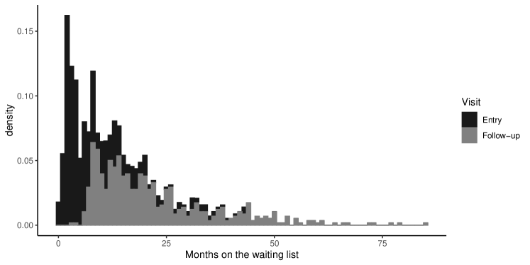
Figure 1: Distribution of the measurement times in the PREDIALA study according to the time since registration on the waiting list (at entry in black and during follow-up in grey)

3.2 The longitudinal IRT model specification

The longitudinal model was defined following equation (1) for the trajectory of underlying depressive symptomatology and equation (2) for the 7 item-specific measurement model. As we did not have any assumption regarding the shape of trajectory over time of depressive symptomatology, we used a basis of natural cubic splines with 2 internal knots placed at tertiles of the measurement time distribution, that is 7 and 15 months, and boundary knots placed at 0 and 60 months. Each of the four functions of time (intercept and 3 splines functions) was associated with fixed effects specific to the group (Preemptive/Dialyzed) to assess the mean trajectories, and individual correlated random effects to account for the correlation within repeated measures of each individual. For the measurement models, we assumed in the main analysis that all items functioned similarly, i.e., no DIF and no response shift occurred. We then explored in secondary analyses whether some items functioned differently by group (adding an item-specific contrast on group), and whether some items were affected by response shift over time (adding an item-specific contrast of the 3 time functions). The parameter estimates of these three models are provided in Table S1 of the supplementary material.

3.3 Predicted trajectories of depressive symptomatology

One unit of depressive symptomatology corresponds to the inter-individual variability at registration in the dialyzed group. In the following description, 1 unit of depressive symptomatology is thus called 1 SD for 1 Standard Deviation.

The predicted mean trajectory over time of depressive symptomatology, displayed in Figure 2, varied according to the group. In the preemptive group, the level of depressive symptomatology increased during the first year on the waiting list by 0.243 (-0.012,0.498) SD and then remained stable. The level of depressive symptomatology was higher in the dialyzed group compared to the preemptive group at the time of registration (difference of -0.482 (-0.814,-0.149) SD). It then slightly decreased during the first year to reach a similar level as in the preemptive group, and then increased again after approximately 2 years on the waiting list by a mean annual rate of 0.245 (0.053,0.438) SD (computed from 2 to 6 years).

Figure 2: Mean trajectory (and 95% confidence interval in shades) of depressive symptomatology estimated by the longitudinal IRT model from the 7 items of HADS repeatedly measured over time; represented for dialyzed and preemptive patients

3.4 Measurement scale structure

We exploited the continuous-time longitudinal IRT model to assess the HADS depressive symptomatology items characteristics. To help appreciating the item characteristics, we assessed the range of the distribution of the underlying depressive symptomatology based on the estimates of the model and an hypothetical population of 100000 preemptive patients and 100000 dialyzed patients with measures every month from registration up to 72 months. The resulting 95% prediction interval of the underlying depressive symptomatology was [-6.10,5.90] with the 10% and 90% percentiles of the distribution at -3.00 and 2.74, respectively.

Table 1 provides the estimated locations and discrimination while Figure 3 shows the curves of item expectations (top) and curves of item information (bottom) according to the underlying depressive symptomatology. Figure S1 and S2 of the supplementary material further display for each item category the probability curve and the information function, respectively.

The items with the lowest location along the latent trait were Item 8 (Slow) and Item 2 (Enjoy) while the item with the highest location along the latent trait was Item 14 (Leisure). This means that the level of depression required to respond to the most unfavorable response categories (i.e. indicative of more severe depressive symptoms) of items 2 and 8 (e.g., “Sometimes” for item 8 “I feel as if I am slowed down”) was lower than the level of depression required to respond to the most unfavorable response categories of item 14 (e.g., “Not often” for item 14 “I can enjoy a good book or radio or TV program”). The most discriminant items with the steepest curves, representing their ability to discriminate patients with different levels of depression, were items 2, 4 and 12 concerning the ability to enjoy, laugh and look forward, respectively. The estimated curve of the Fisher information plotted in Figure 3 (bottom) also underlines the major role of these 3 items compared to the others. In contrast, item 14 about leisure does not bring much information in this population as it seems to measure much higher levels of depression than the other items.

Item	category 0 - 1		category 1 - 2		category 2 - 3		discrimination
	est	SE	est	SE	est	SE	est	SE
2 - Enjoy	-0.46	0.13	0.77	0.14	1.52	0.18	1.29	0.13
4 - Laugh	-0.26	0.12	0.74	0.13	1.91	0.21	1.56	0.16
6 - Cheerful	-0.48	0.14	1.58	0.20	3.34	0.38	0.85	0.09
8 - Slow	-1.51	0.19	0.40	0.13	1.69	0.20	0.95	0.10
10 - Appearance	-0.05	0.12	1.00	0.16	2.27	0.26	0.88	0.10
12 - Looking Forward	-0.32	0.13	0.72	0.13	1.82	0.20	1.46	0.15
14 - Leisure	0.83	0.17	3.18	0.42	4.11	0.54	0.56	0.07

Table 1: Estimate (and associated standard error (SE) obtained by $\Delta$-method) of locations and discrimination of the 7 items of HADS measuring Depressive symptomatology

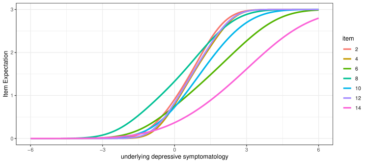
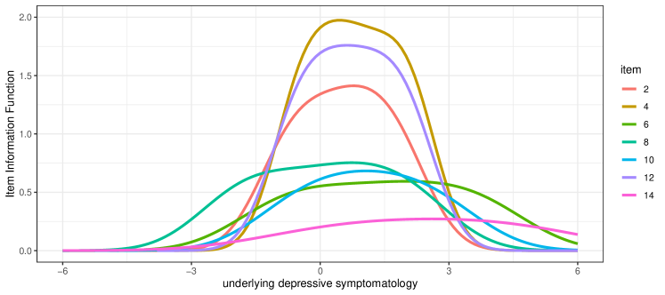
Figure 3: Estimated expectation of each item (top) and estimated Fisher information of each item (bottom) according to the underlying depressive symptomatology. Items are rated so that higher levels systematically indicate more intense depressive symptoms

3.5 Differential Item Functioning and Response Shift

We first explored any differential item functioning on the group (dialyzed versus preemptive). Estimates are provided in Table 2 along with those of the main model that ignores DIF. Overall, the Chi-square test assessing simultaneously the 6 contrasts on group did not reject the null “no DIF on group” assumption (p=0.266). However, taken individually, the difference between groups for item 2 (Enjoy) was significantly larger than for the other items (item-specific effect of preemptive group on the underlying level estimated at -0.150 (-0.269,-0.0314) SD). This suggests that this item has a higher location along the latent trait for preemptive patients (all location parameters shifted to +0.150) as compared to dialyzed patients for a same underlying level of depressive symptomatology; preemptive patients tend to respond more readily to more favorable response categories than patients under dialysis, despite having similar depression levels. In addition, accounting or not for DIF impacted the conclusions: the group effect on the underlying depressive symptomatology was not significant anymore when accounting for DIF suggesting that the difference between groups in the model without DIF was mainly carried by item 2.

		Without DIF on Group				With DIF on Group
		coef	SE	p		coef	SE	p
intercept		0.000	-	-		0.000	-	-
ns1		-0.305	0.172	0.075		-0.304	0.229	0.184
ns2		0.039	0.222	0.862		0.038	0.590	0.949
ns3		0.538	0.250	0.031		0.538	0.310	0.083
group		-0.482	0.170	0.004		-0.458	0.413	0.267
ns1:preemptive		0.477	0.223	0.032		0.473	0.265	0.075
ns2:preemptive		0.428	0.335	0.201		0.429	0.491	0.382
ns3:preemptive		-0.390	0.292	0.182		-0.391	0.338	0.247
Contrasts on preemptive:						(global p=0.266)
Item 2						-0.150	0.061	0.013
Item 4						-0.031	0.059	0.600
Item 6						0.020	0.077	0.800
Item 8						-0.053	0.100	0.593
Item 10						0.040	0.158	0.802
Item 12						0.037	0.061	0.543
* Item 14						0.138	0.124	0.266

** coefficient not estimated but obtained as minus the sum of the others.

Table 2: Estimated fixed parameters in the longitudinal IRT model without (left) and with (right) differential item functioning (DIF) on group. ns1, ns2, ns3 refer to the natural cubic splines functions.

We secondly explored item response shift over time by adding item-specific contrasts on the 3 natural cubic splines functions of time (ns1, ns2, ns3). This resulted in 18 additional parameters (6 contrasts on 3 time functions). Estimates are given in supplementary Table S2. The likelihood ratio test for these 18 parameters, which provides an overall test for RS, did not reject the null hypothesis with a statistic of 22.9 points (p=0.194). The RS was further assessed item by item by testing the 3 item-specific contrasts on time in a multivariate Wald test. Again, no evidence of RS was found for all the items (p$>$0.181) except maybe for item 2 (p=0.073). The predicted trajectories of each item (Figure 4) in the models with and without RS confirmed the absence of substantial response shift over time. Each item behavior over time was close to the one of the underlying construct showed in Figure 2 despite some slight differences in the intensity of change in the first months after entry on the waiting list.

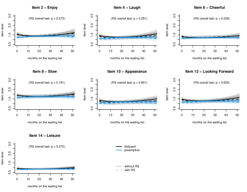
Figure 4: Predicted items trajectories according to time on the waiting list and group in the model neglecting potential response shift (plain) and in the one accounting for potential response shift (dashed) - with p-value of the overall item-specific Wald test for RS over the 3 splines functions in the model assuming RS.

4 Conclusions

We have described how to combine the item response theory with the linear mixed model theory for item-level analysis of longitudinal PRO or CRO data when measurement times may vary across individuals. Using a real case example with the PREDIALA study, we have shown that this longitudinal IRT model can describe the latent construct trajectory over time and its determinants, while simultaneously assessing the item and scale properties, and exploring lack of measurement invariance between groups (DIF) and over time (response shift).

This analysis of PREDIALA data helped to better understand the experience of patients with end-stage renal disease on the renal transplant waiting list in terms of depressive symptoms. DIF was highlighted on item 2 (Enjoy) indicating that patients under dialysis had more difficulty in reporting having enjoyment than preemptive patients, despite having similar levels of depression. This may reveal that the need for clinical and psychological support may not be the same for all patients, according to their renal replacement therapy. Response shift was not significantly evidenced despite a trend on this same item 2. Adjusting for DIF and response shift, the level of depressive symptomatology of preemptive patients tended to slightly increase during the first year and to remain stable afterwards. The level of depressive symptomatology of patients under dialysis tended to be close to the one of preemptive patients after 2 years on the waiting list and to increase afterwards. Although it has been reported that the time on waiting list should be reduced to limit depressive symptoms [26] and improve health-related quality of life [27], the shortage of grafts unfortunately often makes this difficult to achieve.

The longitudinal IRT model we described here unites the strengths of IRT and LMM theories. On the one hand, the use of a structural mixed model makes it possible to operationalize the latent construct as a latent process defined in continuous time and thus takes into account that most health phenomena intrinsically evolve in continuous time. On the other hand, the use of IRT methodology to define the measurement scale at each individual- and occasion-specific observation time enables a precise modeling of the items constituting the measurement scale, and their properties. Longitudinal IRT models had already been proposed in the literature. However, following the usual specification of latent variable models, most of them had considered time as discrete by defining a different latent variable at each measurement occasion (although all these latent variables are supposed to measure the same construct) [8, 9]. In addition to not aligning with the continuous-time nature of health phenomena, it prevents their use in some applications, such as in our study, where measurement times largely vary across subjects. Moreover, neglecting the different lengths of time intervals in longitudinal IRT models may provide biased estimates [28]. The issue of continuous time in longitudinal psychological studies had already been identified in the literature [29] and dealt with by considering continuous-time dynamic systems (with differential equations) to capture the intra-individual serial correlation [28] and implemented in ctsem R package [30]. With the use of a structural mixed model rather than a structural dynamic model, we offer with lcmm R package an alternative approach to flexibly model latent traits in continuous time. We note that, although commercial Mplus software [31] was initially dedicated to discrete-time analyses, it now also offers the posibility to consider time as continuous when defining simple shapes of trajectory (e.g., linear or quadratic), or time as finely discretized with autoregressive structures [32]. The definition of the underlying construct as a latent process evolving in continuous time enables the inclusion of items whatever their measurement timing. These timings can differ from one subject to the other (as shown in the application) and they can differ from one item to the other. We recommend however that the span of measurement times is not too dissimilar, at least for a subset of the items, to ensure that the latent process can be correctly anchored during the entire study time window.

As for all methodologies, the method we propose is not without some limitations and some further path of research may be put forward. First, we focused here on a specific measurement model, the GRM, which translates the discretization of the underlying latent process into ordinal categories as shown in Equation (3) [33]. However, coming from IRT models, this measurement model does not possess the specific objectivity property as Rasch Measurement Theory (RMT) models do [34]. It would thus be interesting to adapt the proposed methodology to RMT measurement models (see Blanchin et al. [35] in this special issue and Barbieri et al. [21]). Of note, changing the measurement model does not impact the estimation procedure nor the structural part of the model, and the current version of the program already handles different measurement models for continuous items in addition to GRM for ordinal items with the possibility to mix continuous and categorical items within the same model.

Second, in the current specification, the serial intra-individual correlation is fully captured by the random effects. Since any type and dimension of time functions can be entered in the model, the method can handle a large variety of structures of intra-individual correlation, whether the data are spaced or frequent. However, in some contexts, considering an additional Gaussian autocorrelation process may be of interest. Although not considered in our work, this could be easily added to the structural linear mixed model as it was previously done with continuous outcomes [17, 18]. Indeed, the added numerical complexity would be low given the use of the quasi Monte-Carlo integral approximation in the log-likelihood which does not vary much with the dimensionality of the random deviations.

Third, by relying on the mixed model theory and the maximum likelihood estimation, the longitudinal IRT model relies on the missing at random assumption both for monotonic and for intermittent missingness [36]. In the presence of informative dropout, a joint model for the repeated item responses and the time to dropout, as described by Saulnier et al.  [20] in this special issue, should be favored. This joint model combines the longitudinal IRT model with a survival model that captures the association between the underlying latent construct and the dropout (or any other event of interest).

Fourth, the methodology is fully parametric, so that analytic choices are systematically made. For instance, to simplify the application setting, we only included time-independent covariates even though time-dependent covariates could also be considered, such as a changing of group during the follow-up. We also globally tested the lack of measurement invariance over the items’ parameters across the overall follow-up although a more precise assessment could be done regarding which function of time is affected or at which time the lack of measurement invariance occurs.

To conclude, by extending the IRT methodology to longitudinal data, and considering the time as continuous, our methodology provides a versatile and flexible approach for modeling item responses measured repeatedly over time as encountered in numerous longitudinal health studies.

Acknowledgements The authors gratefully thank the co-investigators of the study: Magali Giral, Aurélie Meurette, Emmanuel Morelon, and Laetitia Albano. The authors express sincere thanks to Elodie Faurel-Paul and Astrid Fleury for their assistance for the study, as well as all the participants for their contribution to the study. The authors wish to thank members of the clinical research assistant team and DIVAT Consortium Collaborators (Medical Doctors, Surgeons, HLA Biologists). Nantes: Gilles Blancho, Julien Branchereau, Diego Cantarovich, Agnès Chapelet, Jacques Dantal, Clément Deltombe, Lucile Figueres, Claire Garandeau, Magali Giral, Caroline Gourraud-Vercel, Maryvonne Hourmant, Georges Karam, Clarisse Kerleau, Aurélie Meurette, Simon Ville, Christine Kandell, Anne Moreau, Karine Renaudin, Anne Cesbron, Florent Delbos, Alexandre Walencik, Anne Devis; Lyon E. Hériot : Lionel Badet, Maria Brunet, Fanny Buron, Rémi Cahen, Sameh Daoud, Coralie Fournie, Arnaud Grégoire, Alice Koenig, Charlène Lévi, Emmanuel Morelon, Claire Pouteil-Noble, Thomas Rimmelé, Olivier Thaunat.

Funding This work was funded by the French National Research Agency (Project DyMES - ANR-18-C36-0004-01), the French Ministry of Health (PHRC-13-0224, 2013) and by the ”Appel d offres interne analyse secondaire 2018” grant from Nantes University Hospital.

Ethical approval The PREDIALA study is part of the PreKit-QoL study which is registered on the ClinicalTrials.gov Registry (RC14_0078, NCT02154815). It has obtained approval from the ethical Committee for Persons’ Protection (CPP, Tours, 2014-S8), and from the advisory committee on research data and information in health (CCTIRS, Paris, 14.314).

Conflict of interest All authors have no competing interest.

Supplementary Material Supplementary material can be found on the journal website.

Data availability The software is openly available in the R package lcmm (on https://github.com/CecileProust-Lima/lcmm and on cran). The R script along with a dataset mimicking the PREDIALA study are also provided as a package vignette. The raw PREDIALA data can not be shared.

References

- [1] M. Cerou, S. Peigné, E. Comets, M. Chenel, Application of item response theory to model disease progression and agomelatine effect in patients with major depressive disorder, The AAPS journal 22 (1) (2019) 4, pMID: 31720897. doi:10.1208/s12248-019-0379-x.
-
[2]
R. Gorter, J.-P. Fox, J. W. R. Twisk,
Why item response theory
should be used for longitudinal questionnaire data analysis in medical
research, BMC Medical Research Methodology 15 (1) (2015) 55.
doi:10.1186/s12874-015-0050-x.
URL https://doi.org/10.1186/s12874-015-0050-x - [3] W. McCall, B. Porter, A. Pate, C. Bolstad, C. Drapeau, A. Krystal, R. Benca, M. Rumble, M. Nadorff, Examining suicide assessment measures for research use: Using item response theory to optimize psychometric assessment for research on suicidal ideation in major depressive disorder, Suicide & Life-Threatening BehaviorPMID: 34237156. doi:10.1111/sltb.12791.
- [4] G. Abdelhamid, M. Bassiouni, J. Gómez-Benito, Assessing cognitive abilities using the wais-iv: An item response theory approach, International Journal of Environmental Research and Public Health 18 (13) (2021) 6835, pMID: 34202249 PMCID: PMC8297006. doi:10.3390/ijerph18136835.
- [5] S. E. Rakers, M. E. Timmerman, M. E. Scheenen, M. E. de Koning, H. J. van der Horn, J. van der Naalt, J. M. Spikman, Trajectories of Fatigue, Psychological Distress, and Coping Styles After Mild Traumatic Brain Injury: A 6-Month Prospective Cohort Study, Archives of Physical Medicine and Rehabilitation (2021) S0003–9993(21)00462–7doi:10.1016/j.apmr.2021.06.004.
- [6] I. Otto, C. Hilger, A. Magheli, G. Stadler, F. Kendel, Illness representations, coping and anxiety among men with localized prostate cancer over an 18-months period: A parallel vs. level-contrast mediation approach, Psycho-Oncologydoi:10.1002/pon.5798.
- [7] A. Edjolo, C. Proust-Lima, F. Delva, J.-F. Dartigues, K. Pérès, Natural History of Dependency in the Elderly: A 24-Year Population-Based Study Using a Longitudinal Item Response Theory Model, American Journal of Epidemiology 183 (4) (2016) 277–285, number: 4. doi:10.1093/aje/kwv223.
-
[8]
C. Wang, S. W. Nydick, On
Longitudinal Item Response Theory Models: A Didactic, Journal
of Educational and Behavioral Statistics 45 (3) (2020) 339–368, publisher:
American Educational Research Association.
doi:10.3102/1076998619882026.
URL https://doi.org/10.3102/1076998619882026 - [9] L. Cai, C. R. Houts, Longitudinal Analysis of Patient-Reported Outcomes in Clinical Trials: Applications of Multilevel and Multidimensional Item Response Theory, Psychometrika 86 (3) (2021) 754–777. doi:10.1007/s11336-021-09777-y.
- [10] N. M. Laird, J. H. Ware, Random-effects models for longitudinal data, Biometrics 38 (4) (1982) 963–74.
-
[11]
F. Samejima, Graded
Response Model, in: W. J. van der Linden, R. K. Hambleton (Eds.),
Handbook of Modern Item Response Theory, Springer, New York, NY,
1997, pp. 85–100.
doi:10.1007/978-1-4757-2691-6_5.
URL https://doi.org/10.1007/978-1-4757-2691-6_5 - [12] V. Sébille, J.-B. Hardouin, M. Giral, A. Bonnaud-Antignac, P. Tessier, E. Papuchon, A. Jobert, E. Faurel-Paul, S. Gentile, E. Cassuto, E. Morélon, L. Rostaing, D. Glotz, R. Sberro-Soussan, Y. Foucher, A. Meurette, Prospective, multicenter, controlled study of quality of life, psychological adjustment process and medical outcomes of patients receiving a preemptive kidney transplant compared to a similar population of recipients after a dialysis period of less than three years–The PreKit-QoL study protocol, BMC nephrology 17 (2016) 11. doi:10.1186/s12882-016-0225-7.
- [13] L. Auneau-Enjalbert, J.-B. Hardouin, M. Blanchin, M. Giral, E. Morelon, E. Cassuto, A. Meurette, V. Sébille, Comparison of longitudinal quality of life outcomes in preemptive and dialyzed patients on waiting list for kidney transplantation, Quality of Life Research: An International Journal of Quality of Life Aspects of Treatment, Care and Rehabilitation 29 (4) (2020) 959–970. doi:10.1007/s11136-019-02372-w.
- [14] A. Tong, C. S. Hanson, J. R. Chapman, F. Halleck, K. Budde, M. A. Josephson, J. C. Craig, ’Suspended in a paradox’-patient attitudes to wait-listing for kidney transplantation: systematic review and thematic synthesis of qualitative studies, Transplant International: Official Journal of the European Society for Organ Transplantation 28 (7) (2015) 771–787. doi:10.1111/tri.12575.
- [15] P. W. Holland, H. Wainer (Eds.), Differential Item Functioning, Routledge, New-York, NY, 2009.
- [16] M. A. Sprangers, C. E. Schwartz, Integrating response shift into health-related quality of life research: a theoretical model, Social Science & Medicine (1982) 48 (11) (1999) 1507–1515. doi:10.1016/s0277-9536(99)00045-3.
- [17] C. Proust, H. Jacqmin-Gadda, J. M. G. Taylor, J. Ganiayre, D. Commenges, A nonlinear model with latent process for cognitive evolution using multivariate longitudinal data, Biometrics 62 (4) (2006) 1014–1024. doi:10.1111/j.1541-0420.2006.00573.x.
- [18] C. Proust-Lima, H. Amieva, H. Jacqmin-Gadda, Analysis of multivariate mixed longitudinal data: a flexible latent process approach, The British journal of mathematical and statistical psychology 66 (3) (2013) 470–487. doi:10.1111/bmsp.12000.
- [19] F. B. Baker, S. H. Kim, Item Response Theory. Parameter Estimation Techniques, 2nd Edition, Statistics: Textbooks & Monographs, Marcel Dekker, New York, 2004.
-
[20]
T. Saulnier, V. Philipps, W. G. Meissner, O. Rascol, A. Pavy-Le-Traon,
A. Foubert-Samier, C. Proust-Lima,
Joint models for the longitudinal
analysis of measurement scales in the presence of informative dropout,
arXiv:2110.02612 [stat]ArXiv: 2110.02612.
URL http://arxiv.org/abs/2110.02612 -
[21]
A. Barbieri, J. Peyhardi, T. Conroy, S. Gourgou, C. Lavergne, C. Mollevi,
Item response models for the
longitudinal analysis of health-related quality of life in cancer clinical
trials, BMC Medical Research Methodology 17 (1) (2017) 148.
doi:10.1186/s12874-017-0410-9.
URL https://doi.org/10.1186/s12874-017-0410-9 -
[22]
P. Philipson, G. L. Hickey, M. J. Crowther, R. Kolamunnage-Dona,
Faster
Monte Carlo estimation of joint models for time-to-event and multivariate
longitudinal data, Computational Statistics & Data Analysis 151 (2020)
107010.
doi:10.1016/j.csda.2020.107010.
URL https://www.sciencedirect.com/science/article/pii/S0167947320301018 - [23] V. Philipps, B. P. Hejblum, M. Prague, D. Commenges, C. Proust-Lima, Robust and efficient optimization using a Marquardt-Levenberg algorithm with R package marqLevAlg, R journal in press.
-
[24]
C. Proust-Lima, V. Philipps, B. Liquet,
Estimation of Extended Mixed
Models Using Latent Classes and Latent Processes: The R
Package lcmm, Journal of Statistical Software, Articles 78 (2) (2017)
1–56.
doi:10.18637/jss.v078.i02.
URL https://www.jstatsoft.org/v078/i02 - [25] A. S. Zigmond, R. P. Snaith, The hospital anxiety and depression scale, Acta Psychiatrica Scandinavica 67 (6) (1983) 361–370. doi:10.1111/j.1600-0447.1983.tb09716.x.
-
[26]
E. Corruble, A. Durrbach, B. Charpentier, P. Lang, S. Amidi, A. Dezamis,
C. Barry, B. Falissard,
Progressive Increase of
Anxiety and Depression in Patients Waiting for a Kidney
Transplantation, Behavioral Medicine 36 (1) (2010) 32–36, publisher:
Taylor & Francis _eprint: https://doi.org/10.1080/08964280903521339.
doi:10.1080/08964280903521339.
URL https://doi.org/10.1080/08964280903521339 - [27] S. C. Ong, W. L. Chow, S. van der Erf, V. D. Joshi, J. F. Lim, C. Lim, P. S. Tee, Y. M. Lu, T. Y. Kee, What factors really matter? Health-related quality of life for patients on kidney transplant waiting list, Annals of the Academy of Medicine, Singapore 42 (12) (2013) 657–666.
- [28] M. Hecht, K. Hardt, C. C. Driver, M. C. Voelkle, Bayesian continuous-time Rasch models, Psychological Methods 24 (4) (2019) 516–537, place: US Publisher: American Psychological Association. doi:10.1037/met0000205.
- [29] M. C. Voelkle, C. Gische, C. C. Driver, U. Lindenberger, The Role of Time in the Quest for Understanding Psychological Mechanisms, Multivariate Behavioral Research 53 (6) (2018) 782–805, number: 6. doi:10.1080/00273171.2018.1496813.
-
[30]
C. C. Driver, J. H. L. Oud, M. C. Voelkle,
Continuous Time Structural
Equation Modeling with R Package ctsem, Journal of Statistical
Software 77 (2017) 1–35.
doi:10.18637/jss.v077.i05.
URL https://doi.org/10.18637/jss.v077.i05 - [31] B. O. Muthén, L. K. Muthén, Mplus [computer software] (1998-2021).
-
[32]
T. Asparouhov, E. L. Hamaker, B. Muthén,
Dynamic structural
equation models, Structural Equation Modeling: A Multidisciplinary Journal
25 (3) (2018) 359–388.
arXiv:https://doi.org/10.1080/10705511.2017.1406803, doi:10.1080/10705511.2017.1406803.
URL https://doi.org/10.1080/10705511.2017.1406803 - [33] D. Commenges, H. Jacqmin-Gadda, A. Alioum, P. Joly, B. Liquet, C. Proust-Lima, V. Rondeau, R. Thiébaut, Chapter 5. Extensions of mixed models, in: Dynamical Biostastical Models, CRC Press, 2015.
- [34] D. Andrich, Rating scales and rasch measurement, Expert Review of Pharmacoeconomics & Outcomes Research 11 (5) (2011) 571–585, pMID: 21958102. doi:10.1586/erp.11.59.
-
[35]
M. Blanchin, b. priscilla, V. Sébille,
Performance of a
Rasch-based method for group comparisons of longitudinal change and response
shift at item-level in PRO data: a simulation study, working paper or
preprint (Sep. 2021).
URL https://hal.archives-ouvertes.fr/hal-03389050 -
[36]
R. J. A. Little,