CT-ICP: Real-time Elastic LiDAR Odometry with Loop Closure

Abstract

Multi-beam LiDAR sensors are increasingly used in robotics, particularly with autonomous cars for localization and perception tasks, both relying on the ability to build a precise map of the environment. For this, we propose a new real-time LiDAR-only odometry method called CT-ICP (for Continuous-Time ICP), completed into a full SLAM with a novel loop detection procedure. The core of this method, is the introduction of the combined continuity in the scan matching, and discontinuity between scans. It allows both the elastic distortion of the scan during the registration for increased precision, and the increased robustness to high frequency motions from the discontinuity.

We build a complete SLAM on top of this odometry, using a fast pure LiDAR loop detection based on elevation image 2D matching, providing a pose graph with loop constraints. To show the robustness of the method, we tested it on seven datasets: KITTI, KITTI-raw, KITTI-360, KITTI-CARLA, ParisLuco, Newer College, and NCLT in driving and high-frequency motion scenarios. Both the CT-ICP odometry and the loop detection are made available online. CT-ICP is currently first, among those giving access to a public code, on the KITTI odometry leaderboard, with an average Relative Translation Error (RTE) of 0.59% and an average time per scan of 60$ms$ on a CPU with a single thread.

I INTRODUCTION

Many LiDARs are based on the principle of several laser fibers that fire off continuously out of a rotating unit. We call a “scan” the limited time-span aggregation of points covering enough field of view (360 degrees for LiDARs used in autonomous vehicles like in [1, 2]).

To take continuous acquisition into account, LiDAR odometry methods like in [3] or [4] distort the current scan with a constant velocity motion assumption. However, this assumption does not take into account large direction or velocity changes.

On an other hand, recent works like [5, 6] propose real-time LiDAR odometries with continuous-time trajectories. A pose can be calculated for each LiDAR point according to its timestamp from control poses (direct poses or using splines). However, [5] requires an IMU to integrate high-frequency motions, while the continuity constraints in [6] simply smoothes out these motions, we believe, at the cost of precision.

We propose a new elastic formulation of the trajectory with a continuity of poses intra-scan and discontinuity between adjacent scans. In practice, this is defined by solving an elastic scan-to-map registration, parametrized by two poses per scan (for the beginning and end of the scan) with a proximity constraint between the end pose of the previous scan and the beginning pose of the current scan.

Figure 1: Top, in color, one LiDAR scan; the color depends on the timestamp of each point (from the oldest in blue to newest in red). The scan is deformed elastically to align with the map (white points) by the joint optimization of two poses at the start and end of the scan and interpolation according to the timestamp, hence creating a continuous-time scan-to-map odometry. Below, the formulation of our trajectory with a continuity of poses intra-scan and discontinuity between scans.

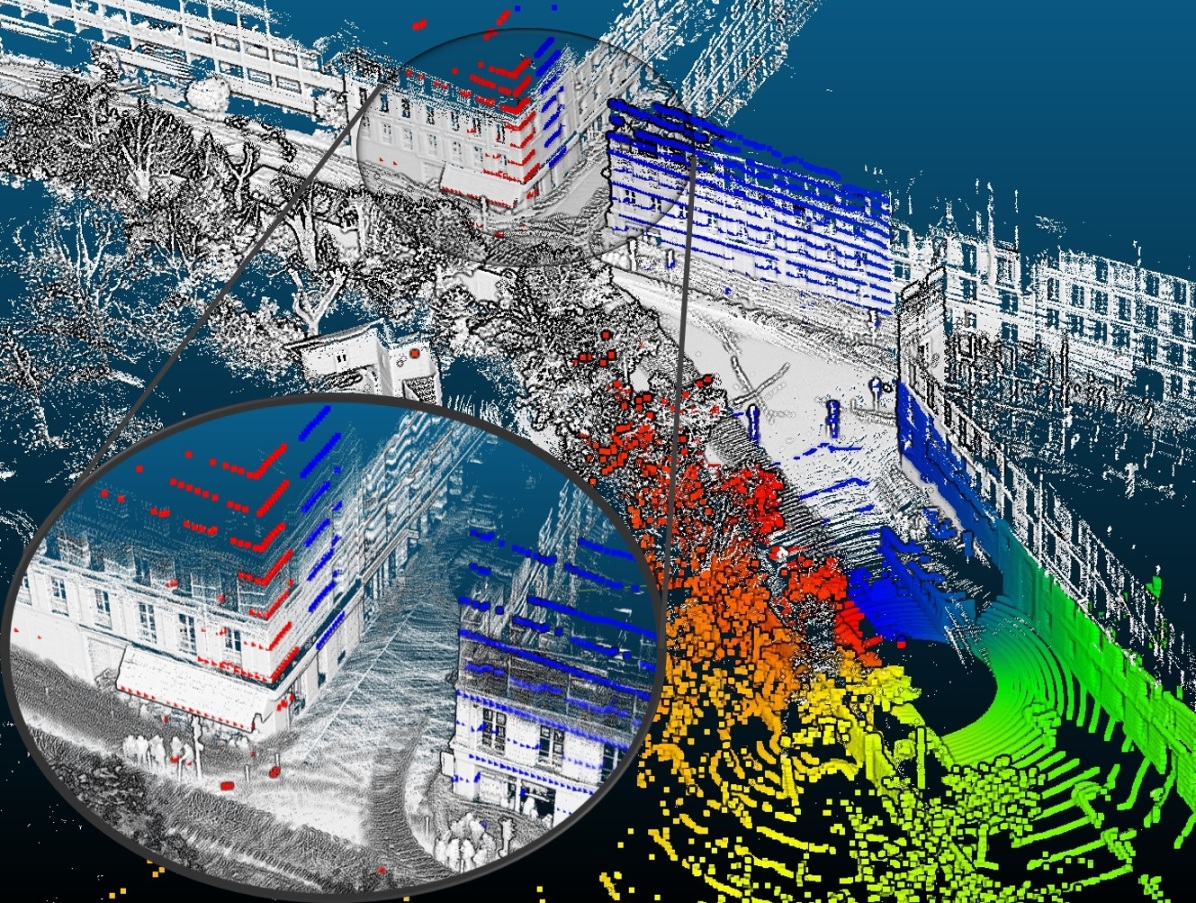
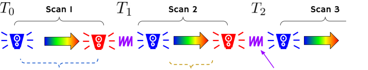
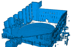
Fig. 1 shows the registration of a scan (points are in color) to the map (points are in white). The color ranges from blue to red, representing the relative timestamp ($\alpha_{i}$) for each point used by our CT-ICP method. Our odometry elastically adjusts the new scan to the building.

As our main contribution, we propose:

• A new elastic LIDAR odometry based on the continuity of poses intra-scan and discontinuity between scans.

We also present as secondary contributions:

• A local map based on a dense point cloud stored in a sparse voxel structure to obtain real-time processing speed.

• A large campaign of experiments on 7 datasets in driving and high-frequency motion scenarios, all reproducible with public and permissive open-source code .

• A fast method of loop detection integrated with a pose graph back-end to build a complete SLAM, integrated into pyLiDAR-SLAM .

II RELATED WORK

Numerous LiDAR odometry methods are based on the Iterative Closest Point (ICP) method [7] and its more efficient point-to-plane variant [8, 9]. KinectFusion [10] for RGB-D sensors has shown great progress in moving from frame-to-frame to frame-to-model registration, likewise, LiDAR odometry methods use scan-to-map registration.

SuMa [11] and SuMa++ [12] represent a scan as an image (range image) and the map in the form of a set of surfels. The registration aligns the current scan with a rendered image obtained by projecting the map of surfels on the GPU. LOAM [13] detects keypoints of different classes (edges, planes) in the range image and registers the detected keypoints into a voxel grid, but the neighborhood search uses separate kd-trees for each class of keypoint. The keypoint map is sufficiently sparse for the search to be carried out in real time. LeGO-LOAM [14] improves on the previous method by separating the keypoints from the ground. F-LOAM [3] has optimized the registration to be faster and runs at more than 20 Hz. More recently, MULLS [4] has improved this approach by detecting the keypoints in the scan in 3D with many different types of keypoints (ground, facade, roof, pillar, beam, and vertex). Differently, IMLS-SLAM [15] represents the map in the form of a dense point cloud, [16] in the form of a TSDF, and PUMA [17] with a mesh, but these last three methods do not work in real time.

To account for sensor movement during scanning, most previous methods like [3, 4, 15] first distort the current scan with a constant velocity motion model from previous poses. Then, the scan distortion is kept fixed during ICP iterations. Although this approach works well in most driving scenarios, it is not robust enough to sudden changes of orientation or fast acceleration from one scan to another.

Another approach takes into account the motion during scanning by defining a continuous-time trajectory with control poses (by linear interpolation or B-splines). CT-SLAM [18] defines the trajectory by using multiple poses per scan; [19] also uses a continuous-time trajectory with six poses per scan (using B-splines basis to represent the trajectory). However, both methods are not in real time. More recently, Elastic LiDAR Fusion in [5] and MARS LiDAR odometry in [6] proposed a continuous-time formulation of the trajectory that operates in real time. [5] uses a linear interpolation of poses with a map of sparse surfels for odometry and dense 2D disk surfels for mapping, while [6] leverages B-splines for the continous-time trajectory with a multi-resolution surfel map to get real-time speed. These methods tend to smooth the trajectory, but in many real-life acquisitions, the motion of the sensor can be shaky (notably due to terrain irregularities) and produce high-frequency movements (with respect to the control point frequencies), which are not taken into account by these methods.

By contrast, CT-ICP defines a continous-time trajectory during the scan and discontinuous between scans. During a scan, the trajectory is parameterized by two poses for the beginning and end of the scan. However, conversely to methods like [6], the final trajectory of CT-ICP is discontinuous, the pose at the beginning of a scan is not equal to the pose at the end of the previous scan. We claim that this approach compensates for the motion irregularities that cannot be compensated for by interpolation.

As precise as it is, LiDAR odometry still accumulates errors in an open environment, which leads to drift in trajectories. A loop closure procedure can correct the trajectories globally, but loop detection is still an open problem for LiDAR SLAM. Currently, most SLAM solutions rely principally on registration methods to directly close loops [20, 11, 13], which only works for small trajectories and low drift. Different place recognition methods have been proposed, operating on individual scans [21, 22, 23, 24], which is sensitive to environment changes and are more adapted for driving scenarios. [4] uses a global registration procedure [25] before ICP-based refinement, but each alignment attempt is very costly, thus restricting the chances to discover more loops. Recently, deep learning methods have been proposed [23, 24], but are not adapted to new environments due to the training requirements. By contrast, we propose a new loop closure procedure that operates on aggregated point clouds projected onto an elevation image. This procedure requires the motion of the sensor to be mostly 2D and to estimate the gravity vector; thus, it can be integrated into any LiDAR odometry for which these conditions are met. Closest to our work is [22], which constructs elevation images but operates on scans, whereas our procedure runs on local maps and, therefore, is not required to test each scan against the previous observed locations, making it more efficient for online SLAM scenarios.

III CT-ICP ODOMETRY

Figure 2: Aggregated point clouds for NCLT dataset (top left), KITTI-CARLA (top-right), Newer College Dataset (bottom left), and ParisLuco (bottom right) show the quality of the maps obtained with CT-ICP.

III-A Odometry formulation

Figure 3: Trajectories estimated with CT-ICP odometry, and our Loop Closure correction (CT-ICP+LC) for the sequences 00 of KITTI-raw (4541 scans), 06 of KITTI-360 (9698 scans), Town01 of KITTI-CARLA (5000 scans), 01_short_experiment of NCD (15301 scans) and 2012-01-08 of NCLT (42764 scans).

Our CT-ICP odometry is parameterized for the current scan by two poses: a pose for the beginning of the scan $\Omega_{b}^{n}=(R^{n}_{b},t^{n}_{b})$ ($R$ for rotation, $t$ for translation, and $b$ for beginning) and a pose for the end of the scan $\Omega_{e}^{n}=(R^{n}_{e},t^{n}_{e})$ ($e$ for end). To simplify the notations, in the following, we omit the $n$ referring to the poses of the current scan. For each sensor measurement captured at a time $\tau\in[\tau_{b},\tau_{e}]$ between the first $\tau_{b}$ and last $\tau_{e}$ timestamp of the scan, the pose of the sensor is estimated by interpolating between the two poses of the scan. These poses transform a point from the LiDAR frame $L(\tau)$ to the world frame $W=L(0)$. Unlike other continuous-time trajectory methods, the pose $\Omega_{b}$ of the new scan does not match the end pose $\Omega_{e}^{n-1}$ of the previous scan. We add a proximity constraint in the optimization to force the two poses to remain close. Our formulation allows our odometry to be more robust to high-frequency motions of the sensor.

For each new scan $\mathbb{S}^{n}$, we first extract a sample of keypoints from $\mathbb{S}^{n}$ indexed by $\mathbb{I}^{n}$: $\{p_{i}\in\mathbb{S}^{n}|i\in\mathbb{I}^{n}\}$ (using a simple grid sampling of points in the scan), that we register into the local map. This map is a dense point cloud $\mathbb{M}^{n}=\{q_{i}^{W}\}$ built from all the previously registered scans, and stored in a sparse voxel grid. Its construction is detailed in section III-B below. Our scan matching then estimates the two optimal poses $\Omega_{b}^{*}$ and $\Omega_{e}^{*}$, thus handling the distortion of the scan during the optimization, and proceeds to transform the points to the world frame before adding them to the local map.

These optimal poses are given by solving the following problem with parameters $\mathbf{X}=(\,\bm{\Omega_{b}},\bm{\Omega_{e}}\,)\in SE(3)^{2}$ in bold:

$$\small\operatorname*{arg\,min}_{\mathbf{X}\in SE(3)^{2}}\;F_{\text{ICP}}(\,\mathbf{X}\,)+\beta_{l}\,C_{\text{loc}}(\mathbf{X})+\beta_{v}\,C_{\text{vel}}(\mathbf{X})$$ (1)

where $F_{\text{ICP}}$ is the scan-to-map continuous-time ICP:

$$F_{\text{ICP}}(\,\mathbf{X}\,)=\frac{1}{|\mathbb{I}^{n}|}\sum_{i\in\mathbb{I}^{n}}\rho(r_{i}^{2}[\mathbf{X}])$$ (2)

And, for each $i\in\mathbb{I}^{n}$,

$$r_{i}[ \mathbf{X}]=a_{i}\;(\,p_{i}^{W}[\mathbf{X}]-q_{i}^{W}\,)\cdot n_{i}$$ (3)

$$p_{i}^{W}[ \mathbf{X}]=R^{\alpha_{i}}[\mathbf{X}]*p_{i}^{L}+t^{\alpha_{i}}[\mathbf{X}]$$ (4)

$$R^{\alpha_{i}}[ \mathbf{X}]=\text{slerp}(\,\mathbf{R_{b}},\,\mathbf{R_{e}},\,\alpha_{i}\,)$$ (5)

$$t^{\alpha_{i}}[ \mathbf{X}]=(1-\alpha_{i})\,\mathbf{t_{b}}+\alpha_{i}\,\mathbf{t_{e}}$$ (6)

$\rho(s)$ is a robust loss function to minimize the influence of outliers, and $r_{i}$ are the residuals of the point-to-plane distance between a sample point $p_{i}^{W}$ and its closest neighbor in the map (as classically formulated by the ICP). $p_{i}^{W}[\mathbf{X}]$ is the point $p_{i}$ expressed in the world frame, $n_{i}$ is the normal of $p_{i}^{W}$’s neighborhood in the local map, and $p_{i}^{L}$ is the sensor measurement (in the LiDAR frame). $\bm{\Omega}^{\alpha_{i}}[\mathbf{X}]=(\mathbf{R^{\alpha_{i}}},\mathbf{t^{\alpha_{i}}})\in SE(3)$ is the transformation from the LiDAR frame at time $\tau_{i}$, $L(\tau_{i})$ to the world $W$. It is estimated by an interpolation between $\bm{\Omega}_{b}$ and $\bm{\Omega}_{e}$ by defining $\alpha_{i}=(\tau_{i}-\tau_{b})/(\tau_{e}-\tau_{b})$. For rotation interpolation, we use the standard spherical linear interpolation (slerp).

We also introduce weights to favor planar neighborhoods: $a_{i}=a_{2D}=(\sigma_{2}-\sigma_{3})/\sigma_{1}$ as defined by [15] (where $\sigma_{i}$ are the square roots of the eigen values of the neighborhood’s covariance), is the planarity of the neighborhood of $p_{i}^{W}$. Note that unlike [15] and most LiDAR odometry methods, we calculate the normals $n_{i}$ and planarity weights $a_{i}$ using the dense point cloud of the local map instead of the current scan, leading to much richer neighborhoods. This computation is done at each iteration of the ICP and for each sample point $p_{i}$, as the refinement on their position leads to more precise neighborhoods.

Additionally in equation 1, we have introduced the two constraints $C_{loc}$ (location consistency constraint), and $C_{vel}$ (constant velocity constraint), with respective weights $\beta_{l}$ and $\beta_{v}$, which is defined as follows:

$$\small C_{loc}(\mathbf{t_{b}}) =||\mathbf{t_{b}}-t_{e}^{n-1}||^{2}$$ (7)

$$C_{vel}(\mathbf{t_{b}},\mathbf{t_{e}}) =||(\mathbf{t_{e}}-\mathbf{t_{b}})-(t_{e}^{n-1}-t_{b}^{n-1})||^{2}$$ (8)

$C_{loc}$ forces the beginning and end location of the sensor to be consistent (limiting the discontinuity), and $C_{vel}$ limits too rapid accelerations. These constraints are sufficient to force the elasticity of CT-ICP to be consistent with the motion model defined implicitly by the weights $\beta_{l}$ and $\beta_{v}$ (taken at 0.001 for all experiments).

CT-ICP performs iterations until a threshold on the norm of parameter’s step is met (typically 0.1 cm on translation and 0.01° in rotation) or a number of iterations is reached (5 to ensure real time). By default, CT-ICP runs on a single thread, but parallel processing (for the construction of the neighborhoods, or while solving the linear system) can be leveraged for more challenging scenarios requiring more iterations and sample points.

III-B Local map and robust profile

As a local map, we use a point cloud from previous scans (like IMLS-SLAM [15]), but in contrast, the points in the world frame ($W$) are stored in a sparse data structure of voxels for faster neighborhood access than kd-trees (constant time access instead of logarithmic). The voxel size of the map controls the radius of the neighborhood search, and the level of detail of the stored point cloud. For driving scenarios, it is set to 1.0 m and 0.80 m for high-frequency motion scenarios, providing satisfying balance between these two aspects.

The voxel size defining the grid of the map is important because it defines the neighborhood search radius, as well as the level of detail of our local map.

Each voxel stores up to 20 points, such that no two points are closer than 10 cm from each other, to limit the redundancy due to the density of measurements along the scan lines. Once a voxel is full, no more points will be inserted into it.

To construct the neighborhood of a point $p_{i}^{W}$ (needed for the computation of $n_{i}$ and $a_{i}$), we select the $k=20$ nearest neighbors among all points in the map in the 27 neighboring voxels from the current point. After running CT-ICP for the current scan $n$, the points are added to the local map. Note that in contrast with pyLiDAR’s F2M, the local map is not based on a sliding window of last scans, but voxels are removed from the map based only on their distance to the center of the last inserted scan.

Odometries with these types of maps are highly sensitive to bad registration, and cannot recover from map pollutions from bad scan insertions. This is particularly problematic in datasets with rapid orientation changes. For these types of datasets, we introduce a robust profile that detects hard cases (fast orientation changes) and registration failures (location inconsistencies or large number of new keypoints falling in empty voxels) and attemps a new registration of the current scan with a more conservative set of parameters (most notably a larger number of sampled keypoints and a larger neighborhood search); for important modifications in the orientation ($\geq 5$ ^∘), we do not insert the new scan in the map, which has a higher probability of being misaligned. The gain in robustness is paid by increased runtime.

IV LOOP CLOSURE AND BACK-END

Figure 4: Qualitative results of loop closure on the sequence 00 of KITTI-360 (11501 scans). The top left is an elevation image built by projecting the local map. The top right shows both the CT-ICP odometry’s trajectory and the one corrected using the computed Loop Closure constraints (CT-ICP+LC). The bottom shows the different loop closure constraints (green) found for the same turn as the local map at the top left.

Our loop closure algorithm maintains in its memory a window of the last scans registered by the odometry. When the window reaches a size of $N_{map}$ scans, the points are aggregated into a point cloud that is placed in the coordinate frame at the center of the window.

Every point of this map is then inserted into a 2D elevation grid, keeping for each pixel the point at a maximum elevation. From this 2D grid, an elevation image is obtained by clipping the $z$ coordinate of each pixel between $z_{min}$ and $z_{max}$. Rotation invariant 2D features [26] are then extracted and saved in memory with the elevation grid. All scans except the last $N_{overlap}$ are dropped from the window.

Every time a new elevation image is built (every $N_{map}-N_{overlap}$ scans), it is matched against the elevation images saved in its memory. A 2D rigid transformation between the two features sets is robustly fit with a RANSAC, and a threshold on the number of inliers is used to validate the correspondences. When a match is validated, an ICP refinement of the initial 2D transform (using Open3D’s ICP [27]) is performed on the elevation grids’ point clouds, producing an accurate 6-DoF loop closure constraint. To reduce the number of candidates, an initial filter selects the $n_{candidates}=10$ candidates closest to the current grid.

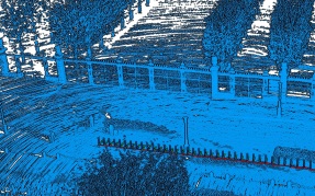
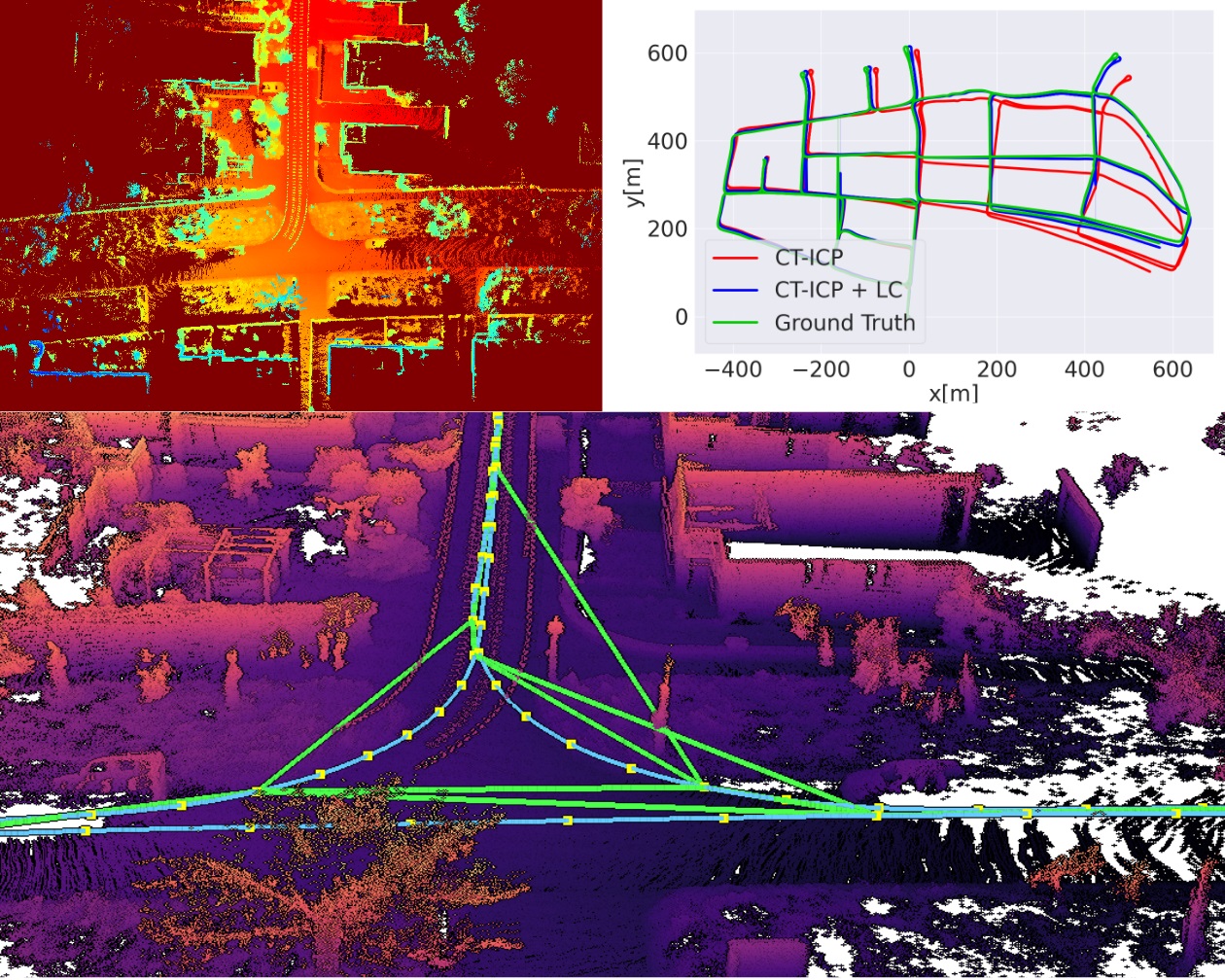
As a back-end, our SLAM uses a standard pose graph (PG) implemented with g2o [28] much like in [20]. The PG regularly adds new poses when new odometry constraints are added with the respective odometry constraints, but the trajectory is only globally optimized when a new loop constraint is detected, in which case the trajectory of the loop closure module is also updated. Fig. 4 summarizes our loop closure procedure.

Currently, our procedure requires the sensor’s motion to be mostly planar on the ground, and for the extrinsic calibration to align the $z$ axis with the normal of the ground plane. This limits the supported sensor setups, as well as the authorized motion. Note that this can be addressed if the gravity vector or the local ground plane are known, in which case the elevation image can be correctly projected. However, we show in section V that for outdoor scenarios with a sensor mostly pointing up, our loop closure detection succeeds in detecting many loops, allowing our back-end to successfully correct the drift errors from the odometry.

V EXPERIMENTS

We demonstrate the efficiency and versatility of our method by conducting experiments on a large variety of datasets: KITTI, KITTI-raw, KITTI-360, KITTI-CARLA, ParisLuco, Newer College Dataset (NCD), and NCLT. Our method requires only the geometry (xyz fields) and the timestamps for each point to elastically distort the scans (they are estimated linearly based on azimuth angles for KITTI-raw and KITTI-360).

V-A Datasets

V-A1 Driving scenarios

KITTI [1] proposes 11 sequences of LiDAR scans acquired from a Velodyne HDL64 mounted on a car and the corresponding ground truth poses from GPS/IMU measurements. The odometry benchmark proposes motion-corrected scans (using the GPS/IMU trajectory to distort the scans): we call this KITTI-corrected. Most odometry methods [13, 11, 15, 4] compare their results on the motion-corrected version of KITTI. However, this does not allow for testing their performance with raw LiDAR data. All odometry sequences (except sequence 03) are available with uncorrected raw scans. We call this KITTI-raw. The same acquisition setup was later used to generate KITTI-360 [29], which contains eight sequences that are much longer than KITTI’s (ranging from 3000 to 15000 scans by sequence) in the same environment. These scans are not motion-corrected, and the timestamps are estimated as described above. For KITTI-corrected, KITTI-raw, and KITTI-360, we applied for all scans an intrinsic angle correction of 0.205 ^∘, as mentioned in [15].

KITTI-CARLA [30] simulates a similar sensor suite as KITTI in a synthetic environment generated using the CARLA simulator [31]. The dataset consists of seven sequences of 5000 scans using a simulated 64-channel LiDAR sensor. The relative motion of the vehicule during the acquisition of the scan is simulated, and each scan provides precise ground truth and timestamps.

ParisLuco is one sequence of 4 km acquisition (12751 scans) in the center of Paris using our own vehicle with a Velodyne HDL32 sensor in a vertical position. We generated the ground truth with post-processing of GPS/IMU measurements (only translations are available).

V-A2 High-frequency motion scenarios

Cars accelerate slowly with respect to the speed of acquisition of the sensor; thus, a constant velocity model is valid. Much more challenging are scenarios were the sensor quickly changes orientations. This is the case for NCLT [32], a dataset containing 27 long sequences ($\geq 20000$ scans per sequence) of scans acquired at Michigan University using a Velodyne HDL32 mounted on a two-wheeled Segway. This dataset is particularly challenging, because the vehicule introduces abrupt rotations to the LiDAR’s own rotation axis, which is problematic for classical ICP-based odometry methods, as shown in [33]

NCD [34], the Newer College Dataset, contains two sequences ($\sim$15000 and $\sim$26000 scans) of a handheld Ouster 64-channel LiDAR mounted on a stick, that is carried accross the Oxford campus.

V-B Odometry Experiments

TABLE I: Relative Translation Error (RTE) [%] with the Driving profile on KITTI-corrected, KITTI-raw, KITTI-360, KITTI-CARLA, and ParisLuco and with the High-Frequency Motion profile on the NCD and NCLT datasets. AVG is the RTE averaged over all segments of all sequences, $\Delta T$ the average running time per scan. KITTI-corrected is the only dataset whose scans have been motion-corrected $(\star)$; all other datasets have uncorrected raw point clouds as scans.

DRIVING PROFILE
KITTI-corrected⋆	00	01		02	03	04		05	06	07		08	09		10		AVG	$\Delta T$
IMLS-SLAM [15]	0.50	0.82		0.53	0.68	0.33		0.32	0.33	0.33		0.80	0.55		0.53		0.55	1250 ms
MULLS [4]	0.56	0.64		0.55	0.71	0.41		0.30	0.30	0.38		0.78	0.48		0.59		0.55	80 ms
pyLiDAR F2M [33]	0.51	0.79		0.51	0.64	0.36		0.29	0.29	0.32		0.78	0.46		0.57		0.53	175 ms
CT-ICP (ours)	0.49	0.76		0.52	0.72	0.39		0.25	0.27	0.31		0.81	0.49		0.48		0.53	60 ms
KITTI-raw	00	01		02	X	04		05	06	07		08	09		10		AVG	$\Delta T$
IMLS-SLAM [15]	0.79	0.86		0.76		0.51		0.48	0.62	0.67		0.97	0.70		0.75		0.71	1070 ms
MULLS [4]	1.43	3.12		1.01		0.57		1.93	1.60	0.69		1.28	1.49		0.71		1.41	80 ms
pyLiDAR F2M [33]	2.20	0.98		1.55		0.45		1.46	0.69	1.72		1.60	1.28		1.18		1.61	530 ms
CT-ICP (ours)	0.51	0.81		0.55		0.43		0.27	0.28	0.35		0.80	0.47		0.49		0.55	65 ms
KITTI-360	00	02		03	04	05		06	07	09		10					AVG	$\Delta T$
IMLS-SLAM [15]	0.65	0.63		0.64	0.89	0.63		0.70	0.54	0.67		0.79					0.68	1060 ms
MULLS [4]	1.60	1.29		0.87	1.64	1.27		1.48	6.25	1.28		0.88					1.55	90 ms
pyLiDAR F2M [33]	1.79	1.25		0.90	1.60	1.26		1.38	0.69	1.72		1.39					1.46	475 ms
CT-ICP (ours)	0.41	0.38		0.34	0.65	0.39		0.42	0.34	0.45		0.69					0.45	70 ms
KITTI-CARLA	Town01		Town02		Town03		Town04		Town05		Town06		Town07				AVG	$\Delta T$
IMLS-SLAM [15]	0.03		0.05		0.16		0.20		0.06		4.90		0.25				0.81	780 ms
MULLS [4]	1.39		0.77		0.69		1.24		1.13		0.98		0.97				1.04	70 ms
pyLiDAR F2M [33]	16.25		7.92		37.16		10.06		9.11		73.29		2.69				23.84	530 ms
CT-ICP (ours)	0.03		0.04		0.03		0.03		0.02		0.04		0.41				0.09	65 ms
ParisLuco	LuxembourgGarden																AVG	$\Delta T$
IMLS-SLAM [15]	1.26																1.26	770 ms
MULLS [4]	3.03																3.03	55 ms
pyLiDAR F2M [33]	4.90																4.90	355 ms
CT-ICP (ours)	1.11																1.11	80 ms
HIGH-FREQUENCY MOTION PROFILE
NCD	01_short_experiment							02_long_experiment									AVG	$\Delta T$
pyLiDAR F2M [33]	1.37							2.63									2.20	1065 ms
CT-ICP (ours)	0.48							0.58									0.55	430 ms
NCLT	2012-01-08																AVG	$\Delta T$
pyLiDAR F2M [33]	19.80																19.80	340 ms
CT-ICP (ours)	1.17																1.17	180 ms

For quantitative evaluations, as in [11, 15, 4, 33], we use the KITTI Relative Translation Error (RTE), which averages the trajectory drift over segments of lengths ranging from 100 m to 800 m. When computing the score on multiple sequences, the average (AVG) is computed over all the segments of all sequences, and mirrors KITTI’s benchmark evaluation.

To compare our method, we evaluated three other LiDAR odometries on the datasets presented: MULLS [4], IMLS-SLAM [15], and pyLIDAR-SLAM F2M [33]. For each of these methods, we searched for the set of parameters offering the best results, but once the parameters are found, we kept the same for all the driving datasets. MULLS and IMLS-SLAM are odometries specialized for driving datasets, which is why we only compared our odometry to pyLIDAR-SLAM F2M [33] on the high-frequency motion datasets NCD and NCLT.

We can see from Table I that all the methods are very close on the KITTI-corrected dataset. However, when we use the uncorrected scans (KITTI-raw and KITTI-360), all the other methods strongly degrade their performance. On the other hand, CT-ICP manages to obtain results very close to those of KITTI-corrected. The corrected scans prevent CT-ICP from using its elastic formulation, but this shows that our map representation and our scan-to-map algorithm are efficient. We also launched our odometry on the KITTI-corrected test sequences (from 11 to 21) and submitted the results online on the KITTI benchmark: we are first among those who put their code online, with a score of 0.59% RTE.

It should be noted that in Table I, we do not obtain the same results published by MULLS on the KITTI-corrected dataset because we are using a single set of parameters for all sequences, whereas MULLS had three different ones (urban, highway, and country).

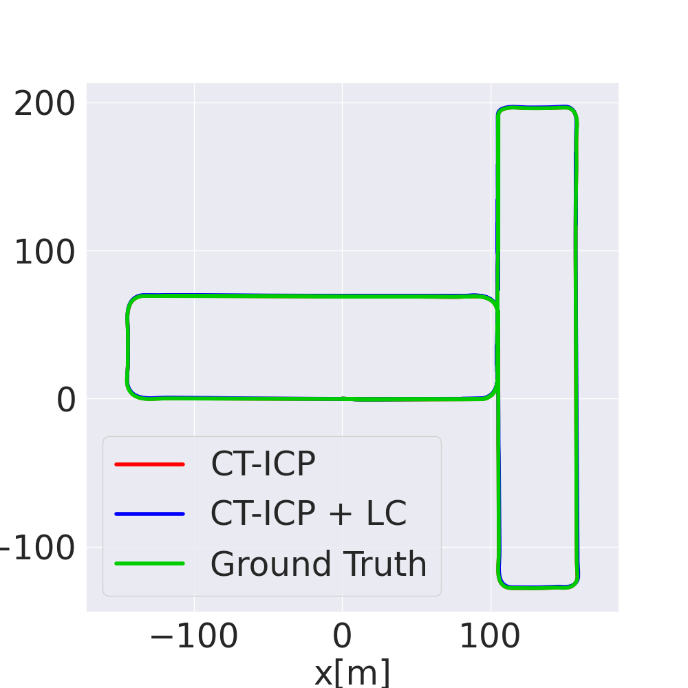
For KITTI-CARLA, a synthetic dataset with scans comprising greater velocity variations than the KITTI datasets (due to the simulated dynamics of the vehicle), the difference between CT-ICP and the other odometries is more obvious: 0.09% RTE for CT-ICP and 0.81% for the best of the three other odometries. This shows the interest of our elastic formulation and discontinuity of poses between scans and how it is able to compensate for small errors in the poses of previous scans.

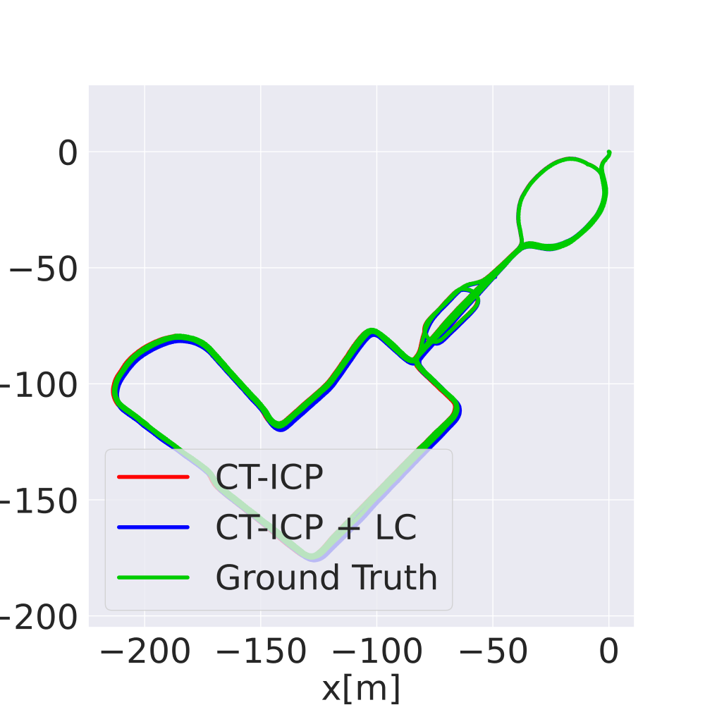
ParisLuco is a dataset with a different sensor (32 fibers instead of 64 for KITTI’s) and low inertia because it was acquired in the center of a city. CT-ICP can overtake IMLS-SLAM, despite using a much sparser map.

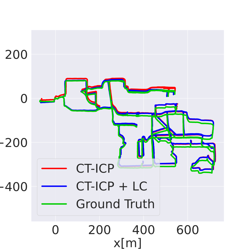
NCD and NCLT are challenging datasets due to the platforms’ unstability (a stick and segway), their lengths (26000 scans for sequence 02_long_experiment, and 46257 scans for sequence 2012-01-08), and the variety of the environments (vegetation, interior, roads, outdoor), and the large number of challenging edge cases. Table I shows that CT-ICP obtains excellent results on NCD (with comparable error rates to KITTI). Further results on NCLT show the robustness of the method because it is able to properly handle all edge cases, resulting in a much lower RTE than pyLiDAR F2M.

To isolate our main contribution, the elastic formulation of CT-ICP, we modified the scan matching of our odometry by distorting the scan with a constant velocity model prior the optimization, and estimated a single pose (while CT-ICP refines the distortion by estimating two poses). We went from 0.55% RTE to 0.79% for KITTI-raw and from 0.45% RTE to 0.60% for KITTI-360, showing a significant loss in precision.

V-C Loop closure experiments

TABLE II: Loop Closure (LC) metrics on one sequence of each dataset. ATE = mean Absolute Trajectory Error [m] after rigid transform is fitted between the ground truth and estimated trajectory, $N_{loop}$ the number of loops detected, LO = LiDAR Odometry

Dataset	Sequence	$N_{loop}$	ATE (LO)	ATE (LO+LC)
KITTI-raw	00	69	6.22	0.66
KITTI-360	00	234	29.87	1.07
KITTI-CARLA	Town01	78	0.21	0.26
ParisLuco	LuxembourgG.	292	29.16	9.65
NCD	01_short_exp.	59	0.22	0.36
NCLT	2012-01-08	520	2.97	2.58

For all datasets, we run CT-ICP with the loop closure module (CT-ICP+LC) with $N_{map}=100$ and $N_{overlap}=30$. For every dataset, we set $z_{min}$ slightly below the ground (using an approximate extrinsic calibration of the sensor) and $z_{max}=z_{min}+10$ m. Finally, for NCLT, we apply a rigid transform to have the default $z$ axis pointing up (instead of down). The computation of each elevation grid and matching of previous ones requires 1.1 s on average, and the pose graph optimization (only launched when a loop constraint is detected) requires an additional 1.2 s on average.

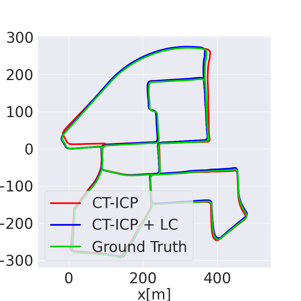
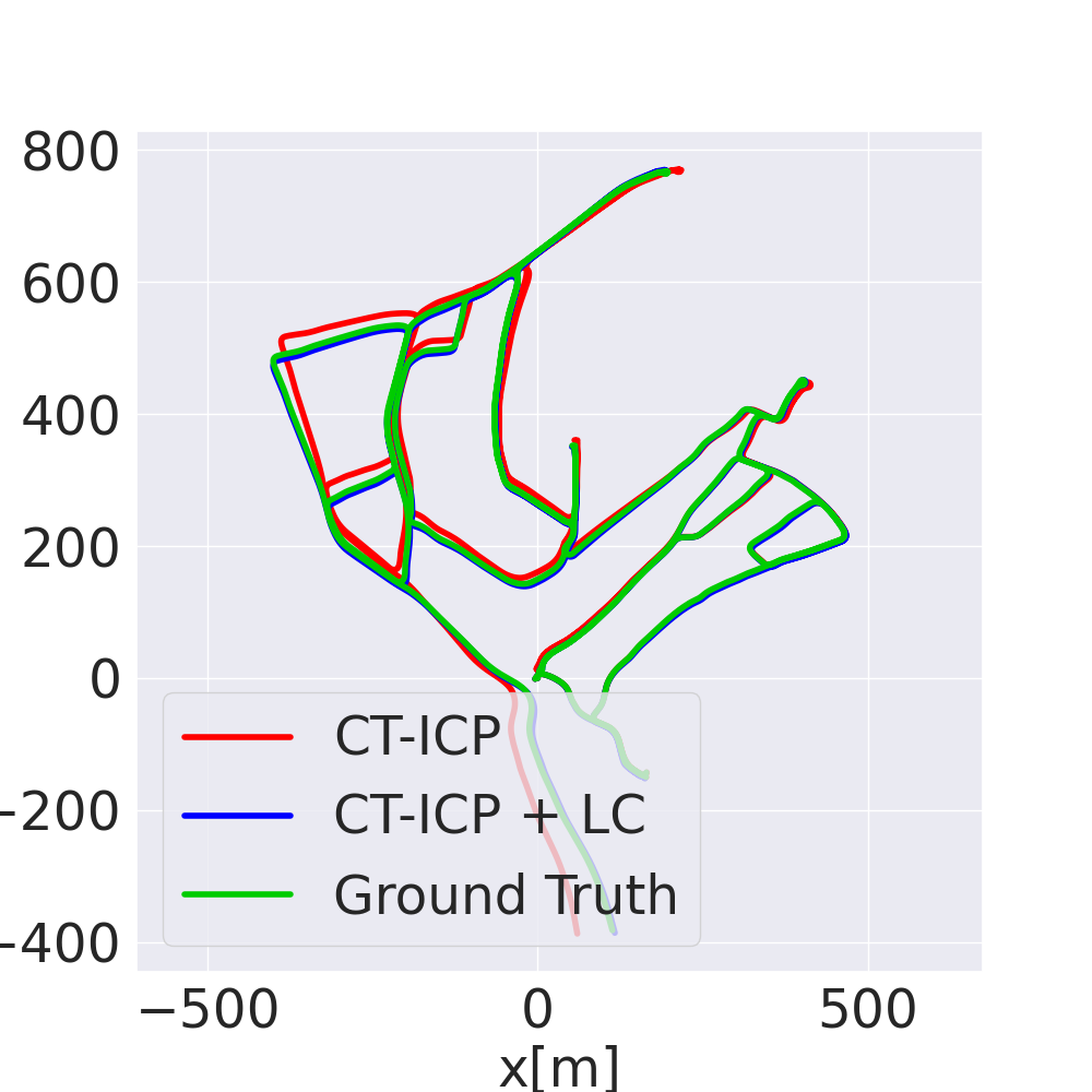
We present qualitative results of our loop closure in Fig. 3 and Fig. 4. To quantitavely evaluate its quality, the RTE is not well suited and tends to deteriorate after loop closure, as noted by [4]. To prove global trajectory improvements, we use the standard Absolute Trajectory Error (ATE) to evaluate our method. However, to decouple the quality assessment from orientation errors in the initial poses, we first estimate the best rigid transform between the ground truth and the estimated trajectory before computing the ATE.

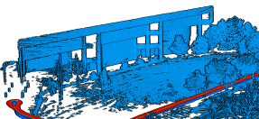
Table II shows the results for a sequence of each dataset. First, we note the great improvement of the ATE after loop closure for KITTI-raw, KITTI-360, and ParisLuco; more so on KITTI-360 because the sequence is much longer. On KITTI-CARLA however, the ATE is almost the same before or after loop closure. This dataset has a very simple geometry, with large and perfect planes, so the challenge to the scan-matching is principally the motion of the sensor during acquisition. CT-ICP manages near-perfect alignments and already leads to 21 cm of precision on the absolute trajectory estimation; this is visualized in Fig. 3, where the ground truth and estimated trajectories are indistinguishable.

Finally, we note the relative large number of loop closure constraints detected for each sequence. This number depends on the frequency of the construction of elevation grids, here as controlled by the size of the overlap $N_{overlap}=30$ and the size of the map $N_{map}=100$. When arriving at an intersection, multiple loop constraints can be computed, as shown in Fig. 4, and with a larger overlap, our method could detect more loop constraints.

VI CONCLUSION

We presented a new real-time LiDAR-only odometry method that goes beyond the state of the art on seven datasets with different profiles, from driving to high-frequency motion scenarios. At the core of our method is the continuous scan matching CT-ICP, which elastically distorts a new scan during the optimization to compensate for the motion during the acquisition. We publish both the code and datasets to allow for the reproduction of all the results presented above. In future work, we will focus on improving our back-end to extend the proposed continuous formulation beyond the scan matching and to fully leverage our loop closure procedure.

References

- [1] A. Geiger, P. Lenz, and R. Urtasun, “Are we ready for autonomous driving? the kitti vision benchmark suite,” in 2012 IEEE Conference on Computer Vision and Pattern Recognition, 2012, pp. 3354–3361.
- [2] H. Caesar, V. Bankiti, A. H. Lang, S. Vora, V. E. Liong, Q. Xu, A. Krishnan, Y. Pan, G. Baldan, and O. Beijbom, “nuscenes: A multimodal dataset for autonomous driving,” arXiv preprint arXiv:1903.11027, 2019.
- [3] H. Wang, C. Wang, C. Chen, and L. Xie, “F-loam: Fast lidar odometry and mapping,” in 2021 IEEE/RSJ International Conference on Intelligent Robots and Systems (IROS), 2020.
- [4] Y. Pan, P. Xiao, Y. He, Z. Shao, and Z. Li, “Mulls: Versatile lidar slam via multi-metric linear least square,” in IEEE International Conference on Robotics and Automation (ICRA), 2021.
- [5] C. Park, P. Moghadam, S. Kim, A. Elfes, C. Fookes, and S. Sridharan, “Elastic lidar fusion: Dense map-centric continuous-time slam,” in 2018 IEEE International Conference on Robotics and Automation (ICRA), 2018, pp. 1206–1213.
- [6] J. Quenzel and S. Behnke, “Real-time multi-adaptive-resolution-surfel 6d lidar odometry using continuous-time trajectory optimization,” arXiv e-prints, p. arXiv:2105.02010, May 2021.
- [7] P. Besl and N. D. McKay, “A method for registration of 3-d shapes,” IEEE Transactions on Pattern Analysis and Machine Intelligence, vol. 14, no. 2, pp. 239–256, 1992.
- [8] S. Rusinkiewicz and M. Levoy, “Efficient variants of the icp algorithm,” in Proceedings Third International Conference on 3-D Digital Imaging and Modeling, 2001, pp. 145–152.
- [9] F. Pomerleau, F. Colas, and R. Siegwart, “A review of point cloud registration algorithms for mobile robotics,” Found. Trends Robot, vol. 4, no. 1, p. 1–104, May 2015. [Online]. Available: https://doi.org/10.1561/2300000035
- [10] R. A. Newcombe, S. Izadi, O. Hilliges, D. Molyneaux, D. Kim, A. J. Davison, P. Kohi, J. Shotton, S. Hodges, and A. Fitzgibbon, “Kinectfusion: Real-time dense surface mapping and tracking,” in 2011 10th IEEE International Symposium on Mixed and Augmented Reality, 2011, pp. 127–136.
- [11] J. Behley and C. Stachniss, “Efficient surfel-based slam using 3d laser range data in urban environments,” in Proceedings of Robotics: Science and Systems (RSS), 2018.
- [12] X. Chen, A. Milioto, E. Palazzolo, P. Giguère, J. Behley, and C. Stachniss, “Suma++: Efficient lidar-based semantic slam,” in 2019 IEEE/RSJ International Conference on Intelligent Robots and Systems (IROS), 2019, pp. 4530–4537.
- [13] J. Zhang and S. Singh, “Low-drift and real-time lidar odometry and mapping,” Auton. Robots, vol. 41, no. 2, p. 401–416, Feb. 2017. [Online]. Available: https://doi.org/10.1007/s10514-016-9548-2
- [14] T. Shan and B. Englot, “Lego-loam: Lightweight and ground-optimized lidar odometry and mapping on variable terrain,” in 2018 IEEE/RSJ International Conference on Intelligent Robots and Systems (IROS), 2018, pp. 4758–4765.
- [15] J.-E. Deschaud, “Imls-slam: Scan-to-model matching based on 3d data,” in 2018 IEEE International Conference on Robotics and Automation (ICRA), 2018, pp. 2480–2485.
- [16] T. Kühner and J. Kümmerle, “Large-scale volumetric scene reconstruction using lidar,” in 2020 IEEE International Conference on Robotics and Automation (ICRA), 2020, pp. 6261–6267.
- [17] I. Vizzo, X. Chen, N. Chebrolu, J. Behley, and C. Stachniss, “Poisson surface reconstruction for lidar odometry and mapping,” in 2021 IEEE International Conference on Robotics and Automation (ICRA), 2021.
- [18] M. Bosse and R. Zlot, “Continuous 3d scan-matching with a spinning 2d laser,” in 2009 IEEE International Conference on Robotics and Automation, 2009, pp. 4312–4319.
- [19] H. Alismail, L. D. Baker, and B. Browning, “Continuous trajectory estimation for 3d slam from actuated lidar,” in 2014 IEEE International Conference on Robotics and Automation (ICRA), 2014, pp. 6096–6101.
- [20] E. Mendes, P. Koch, and S. Lacroix, “Icp-based pose-graph slam,” in 2016 IEEE International Symposium on Safety, Security, and Rescue Robotics (SSRR), 2016, pp. 195–200.
- [21] G. Kim and A. Kim, “Scan context: Egocentric spatial descriptor for place recognition within 3d point cloud map,” in 2018 IEEE/RSJ International Conference on Intelligent Robots and Systems (IROS), 2018, pp. 4802–4809.
- [22] L. Luo, S.-Y. Cao, B. Han, H.-L. Shen, and J. Li, “Bvmatch: Lidar-based place recognition using bird’s-eye view images,” IEEE Robotics and Automation Letters, vol. 6, no. 3, pp. 6076–6083, 2021.
- [23] X. Chen, T. Läbe, A. Milioto, T. Röhling, O. Vysotska, A. Haag, J. Behley, and C. Stachniss, “Overlapnet: Loop closing for lidar-based slam,” in Proceedings of Robotics: Science and Systems (RSS), 2020.
- [24] G. Kim, B. Park, and A. Kim, “1-day learning, 1-year localization: Long-term lidar localization using scan context image,” IEEE Robotics and Automation Letters, vol. 4, no. 2, pp. 1948–1955, 2019.
- [25] H. Yang, J. Shi, and L. Carlone, “Teaser: Fast and certifiable point cloud registration,” IEEE Transactions on Robotics, vol. 37, no. 2, pp. 314–333, 2020.
- [26] J. N. Pablo Alcantarilla and A. Bartoli, “Fast explicit diffusion for accelerated features in nonlinear scale spaces,” in Proceedings of the British Machine Vision Conference. BMVA Press, 2013.
- [27] Q.-Y. Zhou, J. Park, and V. Koltun, “Open3d: A modern library for 3d data processing,” arXiv:1801.09847, 2018.
- [28] R. Kümmerle, G. Grisetti, H. Strasdat, K. Konolige, and W. Burgard, “G2o: A general framework for graph optimization,” in 2011 IEEE International Conference on Robotics and Automation, 2011, pp. 3607–3613.
- [29] J. Xie, M. Kiefel, M.-T. Sun, and A. Geiger, “Semantic instance annotation of street scenes by 3d to 2d label transfer,” in Conference on Computer Vision and Pattern Recognition (CVPR), 2016.
- [30] J.-E. Deschaud, “Kitti-carla: a kitti-like dataset generated by carla simulator,” arXiv e-prints, p. arXiv:2109.00892, Aug. 2021.
- [31] A. Dosovitskiy, G. Ros, F. Codevilla, A. Lopez, and V. Koltun, “Carla: An open urban driving simulator,” in Proceedings of the 1st Annual Conference on Robot Learning, ser. Proceedings of Machine Learning Research, S. Levine, V. Vanhoucke, and K. Goldberg, Eds., vol. 78. PMLR, 13–15 Nov 2017, pp. 1–16. [Online]. Available: http://proceedings.mlr.press/v78/dosovitskiy17a.html
- [32] N. Carlevaris-Bianco, A. K. Ushani, and R. M. Eustice, “University of michigan north campus long-term vision and lidar dataset,” International Journal of Robotics Research, vol. 35, no. 9, pp. 1023–1035, 2015.
- [33] P. Dellenbach, J.-E. Deschaud, B. Jacquet, and F. Goulette, “What’s in my lidar odometry toolbox?” in 2021 IEEE/RSJ International Conference on Intelligent Robots and Systems (IROS), 2021, pp. 4429–4436.
- [34] M. Ramezani, Y. Wang, M. Camurri, D. Wisth, M. Mattamala, and M. Fallon, “The newer college dataset: Handheld lidar, inertial and vision with ground truth,” in 2020 IEEE/RSJ International Conference on Intelligent Robots and Systems (IROS), 2020, pp. 4353–4360.