Abstract

In this paper, we have investigated the physical behavior of cosmological models in the framework of modified Teleparallel gravity. This model is established using a Renyi holographic “dark energy model (RHDE) with a Hubble cutoff. Here we have considered a homogeneous and isotropic Friedman universe filled with perfect ‘fluid. The physical parameters are derived for the present model in Compliances with 43 observational Hubble data sets (OHD). The equation of state (EoS) parameter in terms of $H(z)$ describes a the transition of the universe between phantom and non-phantom phases in the context of $f(T)$ gravity. Our model shows the violation of strong energy condition (SEC) and the weak energy condition (WEC) over the accelerated phantom regime. We also observed that these models occupy freezing regions through $\omega_{D}-\omega_{D}^{{}^{\prime}}$ plane. Consequently, our Renyi HDE model is supported to the consequences of general relativity in the framework of $f(T)$ modified gravity.

Keywords : FLRW universe, Modified Teleparallel gravity, Perfect fluid.

1 Introduction

According to the numerous observations [1, 2, 3, 4], the accelerated expansion of the Universe is due to the presence of an exotic kind of energy, “called dark energy (DE)". The nature and the cosmological origin of DE are still enigmatic. To describe the phenomenon of DE, several models have been presented. According to several findings, DE should behave like a fluid with “negative pressure, counterbalancing the action of gravity, and speeding up the universe"[5, 6, 7]. The general methodology is to define the dynamics of the universe by assuming the source of DE represented as a non-zero “cosmological constant $\Lambda$”, connected to “vacuum quantum field fluctuations”[8, 9, 10].

As proposed by observations, the universe is homogeneous, flat, isotropic, and conforms to FLRW space-time. The existing state of the universe encouraged scientists further to investigate Einstein’s general relativity (GR) to discover the reasons. A cosmological constant is added in GR field equations representing the mysterious form of energy. But it has several drawbacks, like the fine-tuning and the coincidence problems, and its effects are only seen at “cosmological sizes "rather than ‘Planck scales’ [11]. As a result, various modified theories of gravity have been introduced in the literature to overcome the problems with GR. In the framework of modified gravity, it is feasible to change the “Ricci scalar (R)" in the ‘Einstein-Hilbert action’ by arbitrary functions of $R$ [12, 13, 14, 15]. However, namely the “Teleparallel Equivalent of General Relativity (TEGR)" is proposed in the literature [16, 17, 18].

In TEGR, $T$ (torsion scalar) represents the gravitational action. The $f(T)$ gravity is developed as the function of $T$ and extension of TEGR [19, 20, 21]. The estimations of GR agree to coincide with TEGR, while the similar doesn’t occur for $f(T)$ with respect to $f(R)$ gravity [21]. This motivates researchers to propose the various cosmological modifications in $f(T)$ gravity [22]-[31]. Among these, the generalized ‘teleparallel theory of gravity’ has recently attracted much attention as a possible explanation for DE. In this simplification the Lagrangian of teleparallel gravity, the torsion scalar $T$, is changed by its generic function f(T) [27]. The f(T) gravity models utilize the Weitzenb’ock connection, which acquires the torsion and is responsible for the accelerating expansion of the universe [32]. This idea was first proposed by Einstein in 1928 under the name ‘Fern-Parallelismus or teleparallelism’ [33, 34].

The second-order field equations of the $f(T)$ theory have a major advantage over the fourth-order field equations of the f(R) theory [35, 36, 37]. Authors [38] have discussed the detected universe’s acceleration without DE and performed observational viability tests for several $f(T)$ models using SNIa data. Using the Bianchi type I (BI) universe, Sharif and Shamaila [39] developed certain $f(T)$ models. They have also calculated the EoS parameter for ‘two teleparallel models’. Yang developed three new $f(T)$ models and explained their scientific consequences and cosmic behavior [40]. Aly [41] investigated the $f(T)$ gravity in the framework of the THDE. In the same context, Ayman and  Selim worked on the behavior of the fractal cosmology in $f(T)$ gravity[42]. Cosmology of $f(T)$ gravity in a “holographic dark energy and non isotropic" background  discussed in [43].

In $f(T)$  cosmology, Capozziello et al. [44] present a “model-independent approach for numerically solving the modified Friedmann equations". They discussed the behavior of several cosmological parameters with redshift in this hypothesis. In recent studies [45, 46, 47], HDE model has been considered broadly and analyzed as  $\rho\propto\Lambda^{4}$  using the connections between IR, cut off and entropy such that $\Lambda^{3}L^{3}\leq S^{3/4}$. In a similar context, the energy density of HDE model is obtained by the relation of IR cut-offs and ‘Bekenstein-Hawking entropy $S=A/4G$’. The energy density of vacuum depends on the Ricci scalar UV cut-off (particle, event, and Hubble horizons) of the universe and the infrared (IR) cut-off.

A lot of literature is available on the investigations of different IR cut-off [48, 49, 50, 51]. In past few years, various HDE models have been investigated for the cosmological and gravitational incidences using different entropies such as Tsallis [52, 53, 54], Reyni [55, 56] and Sharma-Mittal [57]. Chen [58] introduced recent developments on holographic entanglement entropy. Among these models, a new dark energy model proposed by Moradpour et al. [56] named the Rényi holographic dark energy (RHDE) model for the cosmological and gravitational investigations shows more stability by itself. Several researchers have discussed RHDE in different theories of gravity.

Keeping in view the above motivations, we have investigated the Reyni HDE using the FLRW metric in the context of $f(T)$ modified gravity. The manuscript is arranged in the following manner: In Sect. $2$, the basic equations in $f(T)$ gravity are derived with the framework of the FLRW metric. Renyi’s holographic dark energy model is discussed in Sect. $3$. In Sect. $4$, we have discussed the solutions of the field equations with observational constraints. Sect. $5$ is devoted to the investigation of the energy conditions. In Sect. $6$, we have obtained the $\omega_{D}-\omega_{D}^{{}^{\prime}}$ plane. Sect. $7$ is devoted to the conclusions.

2 Basic Field Equations in f(T) Gravity

The orthonormal tetrad components $e_{A}x^{\mu}$are used to study the teleparallel gravity. Where an index $A$ and $B$ runs over 0, 1, 2, 3 for the tangent space at each point $x^{\mu}$ of the manifold. Their relation to the metric $g_{\mu v}$ is given by

$$g_{\mu\nu}=\eta ABe_{\mu}^{A}e_{\mu}^{B}$$ (1)

where $\mu$ and $\nu$ are coordinate indices on the manifold run over 0, 1, 2, 3, and $e_{\mu}^{A}$ forms the tangent vector of the manifold.

The ‘torsion $T^{\rho}_{\mu\nu}$ and contorsion $K^{\mu\nu}_{\rho}$ tensors’ are read by

$$T^{\rho}_{\mu\nu}\equiv e_{A}^{\rho}(\partial_{\mu}e_{\nu}^{A}-\partial_{\mu}e_{\mu}^{A})$$ (2)

$$K_{\rho}^{\mu\nu}\equiv\frac{-1}{2}(T^{\mu\nu}_{\rho}-T^{\nu\mu}_{\rho}-T^{\mu\nu}_{\rho})$$ (3)

In GR, the Lagrangian density is characterized by the Ricci scalar $R$’, whereas the teleparallel Lagrangian density is described by the  torsion scalar $T$’, which is defined as

$$T\equiv S_{\rho}^{\mu\nu}T^{\rho}_{\mu\nu}$$ (4)

where

$$S_{\rho}^{\mu\nu}\equiv\frac{1}{2}(K_{\rho}^{\mu\nu}+\delta^{\mu}_{\rho}T^{\alpha\nu}_{\alpha}-\delta^{\nu}_{\rho}T^{\alpha\mu}_{\alpha})$$ (5)

Subsequently, the modified teleparallel action for f(T) theory is specified by [33]

$$I=\frac{1}{16\pi G}\int(d^{4}x|e|(T+f(T))$$ (6)

where $T$ is the torsion and $T=-6H^{2}$ and $f(T)$ is a differentiable function of the torsion scalar $T$, $|e|$ = $det(e^{A}_{\mu})$ = $\sqrt{-g}$ and consider $c=16\pi G=1$ . We notices that in the action (6), we have omitted any matter distribution. For more detail derivation giving a clear picture of the relation to relativity.

The space-time metric of Friedmann-Lemaitre-Robertson-Walker (FLRW) is provided by

$$ds^{2}=-dt^{2}+a(t)^{2}dx^{2}$$ (7)

where $a(t)$ is the average scale factor. Using variation, the modified Friedmann equations in $f(T)$ gravity are written as [26]:

$$H^{2}=\frac{1}{3}\rho_{m}-\frac{1}{6}f-2H^{2}f_{T}$$ (8)

$$(H^{2})^{\prime}=\frac{2p_{m}+6H^{2}+12H^{2}f_{T}+f}{24H^{2}f_{TT}-2f_{T}-2}$$ (9)

where, prime represents the derivative with respect to $\ln a$, $f_{T}=\frac{df}{dT}$, $f_{TT}=\frac{d^{2}f}{dT^{2}}$, $\rho_{m}$ is energy density of dark matter and $p_{m}$ is the pressure of dark matter. The modified Friedmann equations in general relativity are given as:

$$H^{2}=\frac{1}{3}\left(\rho_{m}+\rho_{D}\right)$$ (10)

$$(H^{2})^{\prime}=-\left(\rho_{m}+p_{m}+\rho_{D}+p_{D}\right)$$ (11)

For a pressure less dark matter, $p_{m}=0$. On comparing the field Eq.(8)-Eq.(9) with Eq.(10)-Eq.(11), the expression for the energy density $\rho_{D}$ and pressure $p_{D}$ are given as [26]:

$$\rho_{D}=\frac{1}{2}\left(-f+2Tf_{T}\right)$$ (12)

$$p_{D}=\frac{f-Tf_{T}+2T^{2}f_{TT}}{1+f_{T}+2Tf_{TT}}$$ (13)

For our $f(T)$ gravity model, this is the pressure and dark energy density.

3 Renyi Holographic Dark Energy Model

We have consider a $k$ states structure having probability distribution $P_{i}$ and fulfill the condition $\sum_{i=1}^{k}P_{i}=1$. Renyi entropy is a recognized generalized entropy parameter [59].

$$S_{R}=\frac{1}{\delta}ln\sum_{i}^{k}P_{i}^{1-\delta}~{}~{}~{}~{}~{}S_{T}=\frac{1}{\delta}ln\sum_{i=1}^{k}P_{i}^{1-\delta}-P_{i},$$ (14)

where $U\to$ real parameter, $\delta=1-U$. By using Eq. (14), now we have obtain the relation,

$$S_{R}=\frac{1}{\delta}ln(1+\delta S_{T}).$$ (15)

In Eq. (15) the Bekenstein entropy is $S_{T}=\frac{A_{r}}{4}$,   and $A_{r}=4\pi L^{2}$. This gives the Renyi entropy of the system as $S_{R}=\frac{1}{\delta}ln(1+\delta\pi L^{2})$ [56, 60] .

In this model we have taken the Renyi holographic dark energy (RHDE) written as [56],

$$\rho_{{}_{D}}=\frac{3c^{2}}{8\pi GL^{2}}\left(1+\pi\delta L^{2}\right)^{-1}.$$ (16)

The holographic principle (HP) states that the DE density is proportionate to the square of the Hubble parameter, i.e., $\rho_{D}\propto H^{2}$ [61]. According to this principle, the specified choice can resolve the fine-tuning problem. Here the Renyi entropy $S_{R}=\frac{1}{\delta}\ln\left(\frac{\delta}{4}A_{r}+1\right)=\frac{1}{\delta}\ln\left(\pi\delta L^{2}+1\right)$, where $A_{r}=4\pi L^{2}$ and $L=H^{-1}$ is IR cut-off.

The Renyi HDE is obtained as

$$\rho_{{}_{D}}=\frac{3c^{2}}{8\pi G}\frac{H^{2}}{\left(1+\frac{\pi\delta}{H^{2}}\right)}.$$ (17)

4 Solutions of the Field Equations with Observational Constraints

The power-law scale factor is the suitable choice for explaining the matter radiation, and DE-dominated universe. So we choose the scalar of the form Sharma et al. [62] to describe the possible supper accelerated transition.

$$a=\left(nDt\right)^{\frac{1}{n}}$$ (18)

where $n$ and $D$ are positive nonzero constants. From Eq. (18), the Hubble parameter obtained as $H=\frac{\dot{a}}{a}=\frac{1}{nt}$. The following relationship connects the scale factor ($a$) and the redshift ($z$).

$$a=\frac{a_{0}}{(1+z)}$$ (19)

As a result, the Hubble parameter in terms of redshift read as:

$$H(z)=H_{0}(1+z)^{n}$$ (20)

where $H_{0}\to$ present value of Hubble parameter.

In this section, we identify constraints on the model parameters $H_{0}$ and $n$ bounded by the model under the recent $43$ observational Hubble data (OHD) in the range of $0\leq z\leq 1.965$. The data of all 43 H(z) points are compiled in table I of [63, 64]. The reason for using this data is that OHD data produced the cosmic chronometric (CC) technique is model-independent. As detected by observational Hubble data (OHD), the current value of the Hubble constant is $H_{0}=69.45\pm 1.8$ $km/s/Mpc$ and $n=0.7907\pm 0.0687$. We defined $\chi^{2}$ for constraining model parameters $H_{0}$ and $n$ with given as

$$\chi^{2}\left(H_{0},n\right)=\sum_{i=1}^{43}{\frac{\left(H_{th}(i)-H_{ob}(i)\right)^{2}}{\sigma(i)^{2}}}$$ (21)

where $H_{th}(i)$ are the theoretical values of $H(z)$ as per (20) and $\sigma_{i}^{\prime}s$ are errors in the observed values of H(z). The 1- Dimensional marginalized distribution and 2- Dimensional contours with 68.3 $\%$, 95.4 $\%$ and 99.7$\%$ confidence level respectively are obtained for our model as depicted in Fig. $1$.

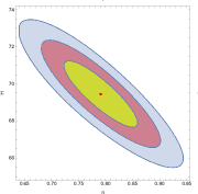
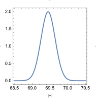
Figure 1: 1-Dimensional marginalized distribution and 2-Dimensional contour plots with best fitted values as $n=0.7907\pm 0.0687$ & $H=69.45\pm 1.8$ in the $n-H$ plane.

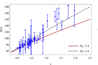
Figure 2: Error bar plots of the Hubble data set

The values of Hubble constant at different redshifts have been estimated by many cosmologists [62, 63, 65] by using the ‘galaxy clustering method and differential age approach’. They determined several observed values of Hubble constant (Hob) along with corrections in the range $0\leq z\leq 1.965$ (Table-1). The observed and theoretical values are found to agree quite well. In the figure-$2$, the dots in this diagram indicate the 43 observed Hubble constant (Hob) values with corrections. The linear curves show the theoretical values of the Hubble constant $(H)$ with marginal corrections.

Table 1: The behaviour of Hubble parameter $H(z)$ with redshift

$S.No$	$Z$	$H(Obs)$	$\sigma_{i}$	References	$S.No$	$Z$	$H(Obs)$	$\sigma_{i}$	References
1	0	67.77	1.30	[66]	24	0.4783	80.9	9	[74]
2	0.07	69	19.6	[67]	25	0.48	97	60	[69]
3	0.09	69	12	[68]	26	0.51	90.4	1.9	[73]
4	0.01	69	12	[69]	27	0.57	96.8	3.4	[77]
5	0.12	68.6	26.2	[67]	28	0.593	104	13	[70]
6	0.17	83	8	[69]	29	0.60	87.9	6.1	[75]
7	0.179	75	4	[70]	30	0.61	97.3	2.1	[73]
8	0.1993	75	5	[70]	31	0.68	92	8	[70]
9	0.2	72.9	29.6	[67]	32	0.73	97.3	7	[75]
10	0.24	79.7	2.7	[71]	33	0.781	105	12	[70]
11	0.27	77	14	[69]	34	0.875	125	17	[70]
12	0.28	88.8	36.6	[67]	35	0.88	90	40	[69]
13	0.35	82.7	8.4	[72]	36	0.9	117	23	[69]
14	0.352	83	14	[70]	37	1.037	154	20	[70]
15	0.38	81.5	1.9	[73]	38	1.3	168	17	[69]
16	0.3802	83	13.5	[74]	39	1.363	160	33.6	[78]
17	0.4	95	17	[68]	40	1.43	177	18	[69]
18	0.4004	77	10.2	[74]	41	1.53	140	14	[69]
19	0.4247	87.1	11.2	[74]	42	1.75	202	40	[69]
20	0.43	86.5	3.7	[71]	43	1.965	186.5	50.4	[78]
21	0.44	82.6	7.8	[75]
22	0.44497	92.8	12.9	[74]
23	0.47	89	49.6	[76]

$$\rho_{D}=\frac{6c^{2}H_{0}^{4}(z+1)^{4n}}{\pi\delta+H_{0}^{2}(z+1)^{2n}}$$ (22)

Solving Eqs. (22), (9) and (12), we get:

$$f(T) = -6\sqrt{-H_{0}^{2}(z+1)^{2n}}\bigg{[}2\sqrt{\pi}c^{2}\sqrt{\delta}\tanh^{-1}\left(\frac{\sqrt{-H_{0}^{2}}}{\sqrt{\pi}\sqrt{\delta}}\right)-2\sqrt{\pi}c^{2}\sqrt{\delta}$$ (23)

$$\times \tanh^{-1}\left(\frac{\sqrt{-H_{0}^{2}(z+1)^{2n}}}{\sqrt{\pi}\sqrt{\delta}}\right)+2c^{2}\sqrt{-H_{0}^{2}(z+1)^{2n}}-(1+2c^{2})\sqrt{-H_{0}^{2}}\bigg{]}$$

Here Eq. (23) represents the $f(T)$ function for proposed model. From Eq. (13), the pressure for the model determined as:

$$p_{D}=\frac{12\pi c^{2}\delta H_{0}^{4}(z+1)^{4n}}{-2\pi\left(2c^{2}-1\right)\delta H_{0}^{2}(z+1)^{2n}+\left(1-2c^{2}\right)H_{0}^{4}(z+1)^{4n}+\pi^{2}\delta^{2}}$$ (24)

By using Eqs. (22) and (24) the equation-of-state parameter $\omega_{D}$ is given by

$$\omega_{D}=\frac{\pi\delta\left(6\pi\delta+6H_{0}^{2}(z+1)^{2n}\right)}{-6\pi\left(2c^{2}-1\right)\delta H_{0}^{2}(z+1)^{2n}+3\left(1-2c^{2}\right)H_{0}^{4}(z+1)^{4n}+3\pi^{2}\delta^{2}}$$ (25)

The dark energy density parameter $\Omega_{D}$ is given by

$$\Omega_{D}=\frac{c^{2}H_{0}^{2}(z+1)^{2n}}{\pi\delta+H_{0}^{2}(z+1)^{2n}}$$ (26)

We can obtain $\omega_{D}^{{}^{\prime}}$ and $\Omega_{D}^{{}^{\prime}}$ by differentiating Eqs. (25) and (26) with respect to $\log a$ :

$$\omega^{{}^{\prime}}_{D} = 4\pi\delta H_{0}^{2}n(-z-1)(z+1)^{2n-1}\bigg{[}\pi^{2}\left(4c^{2}-1\right)\delta^{2}$$ (27)

$$+ \left(2c^{2}-1\right)H_{0}^{2}(z+1)^{2n}\bigg{(}2\pi\delta+H_{0}^{2}(z+1)^{2n}\bigg{)}\bigg{]}/\bigg{[}2\pi\left(2c^{2}-1\right)\delta H_{0}^{2}(z+1)^{2n}$$

$$+ \left(2c^{2}-1\right)H_{0}^{4}(z+1)^{4n}-\pi^{2}\delta^{2}\bigg{]}^{2}$$

$$\Omega^{{}^{\prime}}_{D}=-\frac{2\pi c^{2}\delta H_{0}^{2}n(z+1)^{2n}}{\left(\pi\delta+H_{0}^{2}(z+1)^{2n}\right){}^{2}}$$ (28)

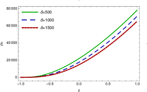
Figure 3: Variation of DE $\rho_{D}$ versus $z$

The evolution of dark energy density with redshift is depicted in Figure $3$ for various values of $\delta$, we can see that dark energy density ($\rho_{D}$) is a positive decreasing function of redshift throughout the evolution of the universe at the present epoch.

Figure 4: Variation of $p_{D}$ versus $z$

We have noticed in Figure 4 that the pressure decreases as the redshift increases. The pressure remains negative through the evolutionary era and approaches zero in the high redshift area. It has been hypothesized that the cosmic acceleration is caused by negative pressure as confirmed by recent estimations.

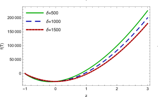
Figure 5: Variation of $f(T)$ versus $z$

The behavior of $f(T)$ versus redshift is shown in Figure $5$. It is observed that $f(T)$ has an expanding behavior over the specified range. Various values of $\delta$, start with a high negative value and gradually approach a positive value.

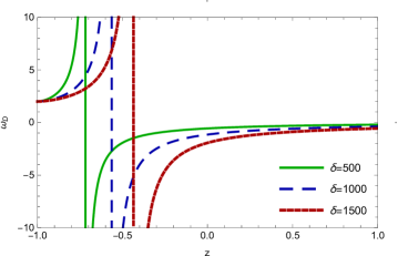
Figure 6: Variation of $\omega_{D}$ versus $z$

In Figure 6, we observed the dynamics of the EoS parameter against redshift ($z$) for various esteems of $\delta$ = 500, 1000, 1500. The EoS parameter classifies the expansion of the universe. The values of EoS parameter $-1<\omega_{D}\leq 0$,  $\omega_{D}=-1$ and $\omega_{D}<-1$ represents the quintessence , $\Lambda$CDM and Phantom eras respectively. In the derived model, EoS parameter $\omega_{D}$ starts with ‘quintessence era’, crosses the phantom divide line, and enters in the phantom era [79, 80, 81]. The graph predicted that the universe is under the influence of $\Lambda CDM$. It is well known that for an accelerating universe, we should have $\omega_{D}<-1/3$. In the later time, it shows the ‘stiff fluid’ when $\omega_{D}=1$, the matter-dominated phase when $\omega_{D}=0$ and $\omega_{D}=1/3$ represents the radiation dominated phase [19, 82].The graph demonstrates that dark energy is influencing the universe, as the equation of state predicts an accelerated expansion phase. It’s worth noting that this type of crossover behavior is consistent with current cosmic observational findings.

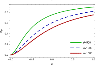
Figure 7: Variation of $\Omega_{D}$ versus $z$

The density parameter ($\Omega_{D}$) for the RHDE models are depicted in Figure 7 for different values of $\delta$ [83, 84]. Dark energy dominates the late universe and gradually evolves to $\Omega$ = 1 in the future. Here $\Omega$ is the total density parameter. It is worth noting that the density parameter is decreasing in a good direction [83, 84, 85].

5 Energy Conditions

The energy conditions (ECs) are significant techniques for explaining the Universe’s geodesics. If we are working with a perfect fluid matter distribution the energy conditions recovered from conventional GR.

There are various types of energy conditions:

• Null Energy Condition (NEC): $\rho\geq 0$

• Weak Energy Condition (WEC): $\rho+p\geq 0$

• Dominant Energy Condition (DEC): $\rho-p\geq 0$

• Strong Energy Condition (SEC): $\rho+3p\geq 0$.

All of the above expression for energy conditions are depend on the model parameters.

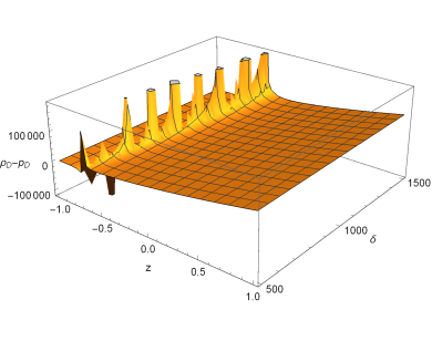
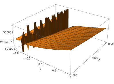
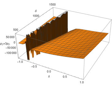
Figure 8: Variation of $\omega_{D}^{{}^{\prime}}$ versus $z$

Figure 8 shows the plots of energy conditions vs. redshift. The violation of SEC is generally due to the anti-gravity matter such as dark energy present in the universe. For normal matter, all the energy conditions including SEC must be validated. In the derived model, Fig. 8 shows the validation and violation of energy conditions for the particular choice of free parameters and satisfied the energy conditions. The WEC and DEC are satisfied initially, but both violate at the present epoch. But it is observed that the SEC does not satisfy $f(T)$ gravity. In the fact, these energy conditions are crucial in comprehending cosmic scenarios [86, 87]. The Hawking-Penrose singularity theorems are primarily studied using WEC and SEC. The SEC is critical to comprehending the allure of gravity [88, 89]. Now the violation of SEC, indicates clearly the expansion of the universe with acceleration which proves the correctness of the derived model.

6 $\omega_{D}-\omega_{D}^{{}^{\prime}}$ plane

The authors [90, 91] were developed the $\omega_{D}-\omega_{D}^{{}^{\prime}}$ plane to examine the cosmic evolution of the quintessence dark energy concept. Figure 9 illustrates the phase plane dynamics of the models with $\delta=500,1000,1500$ and have freezing like models $\omega_{D}\geq-1$. We have observed that our RHDE model lies freezing region ($\omega_{D}<0$ , $\omega_{D}^{{}^{\prime}}<0$ ).

Figure 9: Plot of $\omega_{D}-\omega^{\prime}_{D}$.

It has been found that the universe’s cosmic expansion accelerates more rapidly in the freezing area. In the context of $f(T)$ modified gravity, the graphical behavior displayed ($\omega_{D}^{{}^{\prime}}<0$ ) suggested that the Renyi HDE model is in the freezing region and cosmic expansion are more accelerated.

7 Conclusions

Using $46$ OHD points, we have calculated the cosmological parameter values of the resultant models in the present paper. Energy density, pressure, the $f(T)$ function, the equation of state parameter, and the $\omega_{D}-\omega_{D}^{{}^{\prime}}$ cosmic plane have all been examined. In terms of redshift, we have obtained all these cosmological parameters here. It is demonstrated in the current research that these results are compatible with the observation data. The following are the model’s key characteristics:

• 1-Dimensional marginalized distribution and 2-Dimensional contour plots and Error bar plots of the Hubble data set are shown in Figs. $1$ $\&$ $2$. We obtained throughout the evaluation, that the energy density is positive and the pressure is negative, as seen in Figs. $3$ $\&$ $4$. The energy density must be positive, and the pressure must be negative for cosmic acceleration. The evolution of pressure and energy density of our model satisfies WEC. This type of character can only be obtained by modified general relativity or exotic matter.

• We have determined that $f(T)$ is the uniformly expanding function in our model (see Fig. $5$).

• The EoS parameter $\omega_{D}$ is a crucial parameter describing the various matter-dominated phases of the universe’s evolution. The overall effect of the EoS parameter demonstrates that the universe began at $\omega_{D}=0$ (goes up to negative values and represents the universe’s acceleration), then gradually increases to a positive deceleration phase. Subsequently, it proceeds to the accelerated era, the second phase of the universe’s current acceleration. As a result, our derived model is found in both the quintessence and phantom regions (see Fig. $6$).

• We have investigated the evolution of dark energy by observing the behaviour of $\Omega_{D}$. We noticed that $\Omega_{D}$ is positive decreasing functions (see Fig. 7).

• We have shown how the energy conditions (ECs) are changing with time. It is important to mention here that the SEC must violate to support the universe’s late-time acceleration, and Fig. 8 shows that SEC is not satisfied.

• Additionally, the $\omega_{D}-\omega_{D}^{\prime}$ plane revealed that the Renyi HDE model lies in the freezing region for various values of $\delta$ during the evolution (see Fig. $9$). In the framework of $f(T)$ modified gravity, the cosmic expansion will be more accelerated.

As a result, in the framework of $f(T)$ gravity, general relativity results are consistent with the Renyi HDE model. We note that the dark energy issue may be simply represented in Teleparallel gravity as a geometric term. The scientists who are engaged in this subject are intrigued by this fact.

References

- [1] S. Perlmutter et al., Measurements of 4 and from 42 high-redshift supernovae, Astrophys. J 517 (1999) 565 .
- [2] R. A. Knop et al. , New constraints on , , and from an independent set of 11 high-redshift supernovae observed with the Hubble Space Telescope, Astroph. J. 598 (2003) 102.
- [3] D. N. Spergel et al.,Three-year Wilkinson Microwave Anisotropy Probe (WMAP) observations: implications for cosmology, Astroph. J. Suppl. 170 (2007) 377.
- [4] A. G. Riess et al.,Observational evidence from supernovae for an accelerating universe and a cosmological constant, Astron. J. 116 (1998) 1009.
- [5] S. Perlmutter et al., Measurements of and from high-redshift supernovae, Astrophys. J 17 (1999) 565.
- [6] P. A. R. Ade et al., Planck 2015 results. XIII. Cosmological parameters,Astron. Astrophys. 594 (2016) A13.
- [7] E. J. Copeland, M. Sam and S. Tsujikawa, Dynamics of dark energy, Int. J. Mod. Phys. D 15 (2006) 1753.
- [8] S. Perlmutter et al., Discovery of a supernova explosion at half the age of the Universe, Nature 391 (1998) 51.
- [9] B. P. Schmidt et al., The high-Z supernova search: measuring cosmic deceleration and global curvature of the universe using type Ia supernovae, Astrophys. J. 507 (1998) 46.
- [10] A. G. Riess et al., Type Ia supernova discoveries at from the Hubble Space Telescope: Evidence for past deceleration and constraints on dark energy evolution, Astrophys. J. 607 (2004) 665.
- [11] S. Carlip, Hiding the cosmological constant, Phys. Rev. Lett. 123 (2019) 131302.
- [12] S. Capozziello and M. De Laurentis, Extended theories of gravity, Phys. Rep. 509 (2011) 167.
- [13] L. M. Krauss and J. B. Dent, Higgs seesaw mechanism as a source for dark energy, Phys. Rev. Lett. 111 (2013) 061802.
- [14] S. I. Nojiri and S. D. Odintsov, Unified cosmic history in modified gravity: from theory to Lorentz non-invariant models, Phys. Rep. 505 (2011) 59.
- [15] A. De Felice and S. Tsujikawa, f(R) theories, Living Rev. Rel. 13 (2010) 1.
- [16] A. Einstein, Riemannian geometry with maintaining the notion of distant parallelism, Sitz. Preuss. Akad. Wiss 217 (1928).
- [17] R. Aldrovandi and J. G. Pereira, Why to study teleparallel gravity, In Teleparallel Gravity, Springer, Dordrecht (2013) 179.
- [18] J. W. Maluf, The teleparallel equivalent of general relativity, Ann. Phys. 525 (2013) 339.
- [19] Y. F. Cai, S. Capozziello, M. De Laurentis and E. N. Saridakis, teleparallel gravity and cosmology, Rep. Prog. Phys. 79 (2016) 106901.
- [20] K. Atazadeh and F. Darabi, cosmology via Noether symmetry. Eur. Phys. J. C 72 (2012) 1.
- [21] R. Ferraro and F. Fiorini, Born-Infeld gravity in Weitzenböck spacetime, Phys. Rev. D 78 (2008) 124019.
- [22] S. H. Chen, J. B. Dent, S. Dutta and E. N. Saridakis, Cosmological perturbations in gravity, Phys. Rev. D 83 (2011) 023508.
- [23] J. B. Dent, S. Dutta and E. N. Saridakis, f (T) gravity mimicking dynamical dark energy. Background and perturbation analysis, JCAP 01 (2011) 009.
- [24] K. Bamba, R. Myrzakulov, S.I. Nojiri and S. D Odintsov, Reconstruction of f (T) gravity: rip cosmology, finite-time future singularities, and thermodynamics, Phys. Rev. D 85 (2012) 104036.
- [25] V. F. Cardone, N. Radicella and S. Camera, Detectability of torsion gravity via galaxy clustering and cosmic shear measurements, Phys. Rev. D 89 (2014) 083520.
- [26] K. Bamba, C. Q. Geng, C. C. Lee and L. W Luo, Equation of state for dark energy in gravity, JCAP 01 (2011) 021.
- [27] M. Sharif and S. Rani, F (T) models within bianchi type-I universe, Mod. Phys. Lett. A 26 (2011) 1657.
- [28] M. R. Setare and M. J. S Houndjo, Finite-time future singularity models in gravity and the effects of viscosity, Can. J. Phys. 91 (2012) 260.
- [29] J. Amoros, J. de Haro and S. D. Odintsov, Bouncing loop quantum cosmology from gravity, Phys. Rev. D 87 (2013) 104037.
- [30] V. Fayaz, H. Hossienkhani, A. Farmany, M. Amirabadi and N Azimi, Cosmology of gravity in a holographic dark energy and nonisotropic background, Astrophys. Space Sci. 351 (2014) 299.
- [31] A. Sepehri, A. Pradhan, A. Beesham and J. de Haro, Teleparallel loop quantum cosmology in a system of interecting branes, Phys. Lett. B 760 (2016) 94.
- [32] R. Myrzakulov, Accelerating universe from gravity, Eur. Phys. J. C 71 (2011) 1
- [33] E. V. Linder, Einstein’s Other Gravity and the Acceleration of the Universe, Phys. Rev. D 81 (2010) 127301.
- [34] A. Unzicker, T. Case, Translation of Einstein’s attempt of a Unified field theory with teleparallelism, arXiv:physics/0503046 [physics.hist-ph].
- [35] M. Sharif and A. Jawad, Interacting modified holographic dark energy in Kaluza-Klein universe, Astrophys. Space Sci. 337 (2012) 789.
- [36] M. Sharif and H. R. Kausar, Effects of dark energy on dissipative anisotropic collapsing fluid, Mod. Phys. Lett. A 25 (2010) 3299.
- [37] M. Sharif and H. R. Kausar, Gravitational perfect fluid collapse in gravity, Astrophys. Space Sci. 331 (2011) 281.
- [38] G. R. Bengochea and R. Ferraro, Dark torsion as the cosmic speed-up, Phys. Rev. D 79 (2009) 124019.
- [39] M. Sharif and H. R. Kausar, Non-vacuum solutions of Bianchi type universe in gravity, Astrophys. Space Sci. 332 (2011) 463.
- [40] R. J. Yang, New types of gravity, Eur. Phys. J. C 71 (2011) 1797.
- [41] A. A. Aly, Study of gravity in the framework of the Tsallis holographic dark energy model, Eur. Phys. J. Plus 134 (2019) 1.
- [42] A. A. Aly and M. M. Selim, Behaviour of dark energy model in fractal cosmology, Eur. Phys. J. Plus 130 (2015) 1-7.
- [43] V. Fayaz, et al., Cosmology of gravity in a holographic dark energy and nonisotropic background, Astrophys Space Sci. 351 (2014) 299.
- [44] S. Capozziello, R. D. Agostino, and O. Luongo, Model-independent reconstruction of teleparallel cosmology, Gen. Rel. Gravit. 49 (2017) 1.
- [45] M. Li, A model of holographic dark energy, Phys. Lett. B 603 (2004) 1.
- [46] A. Sheykhi, Holographic scalar field models of dark energy, Phys. Rev. D 84 (2011) 107302.
- [47] Y. Z. Ma, Y. Gong and X. Chen, Features of holographic dark energy under combined cosmological constraints, Eur. Phys. J. C 60 (2009) 303.
- [48] C. Gao , F. Wu et al., Holographic dark energy model from Ricci scalar curvature, Phys. Rev. D 79 (2009) 043511.
- [49] L. N. Granda and A. Oliveros, New infrared cut-off for the holographic scalar fields models of dark energy, Phys. Lett. B 671 (2009) 199.
- [50] K. Karami and J. Fehri, New holographic scalar field models of dark energy in non-flat universe, Phys. Lett. B 684 (2010) 61.
- [51] S. Wang and Y. Wang et al., Holographic dark energy, Phys. Rept. 696 (2017) 1.
- [52] M. Tavayef, A. Sheykhi, K. Bamba and H. Moradpour, Tsallis holographic dark energy, Phys. Lett. B 781 (2018) 195.
- [53] A. Dixit, U. K. Sharma and A. Pradhan, Tsallis holographic dark energy in FRW universe with time varying deceleration parameter, New Astronomy 73 (2019) 101281.
- [54] A. Pradhan and A. Dixit, Tsallis holographic dark energy model with observational constraints in the higher derivative theory of gravity, New Astronomy 89 (2021) 101636.
- [55] A. Dixit, V. K. Bhardwaj and A. Pradhan, RHDE models in FRW Universe with two IR cut-offs with redshift parametrization, Eur. Phys. J. Plus 135 (2020) 1.
- [56] H. Moradpour, S. A. Moosavi, I. P. Lobo, J. P. Morais Graa, A. Jawad and I. G. Salako, Thermodynamic approach to holographic dark energy and the Rényi entropy, Eur. Phys. J. C 78 (2018) 1.
- [57] A. Sayahian Jahromi, S. A. Moosavi, H. Moradpour, J. P. Morais Graa, I. P. Lobo, I. G. Salako and A. Jawad, Generalized entropy formalism and a new holographic dark energy model, Phys. Lett. B 780 (2018) 21.
- [58] B. Chen, Holographic Entanglement Entrop, Commun. Theor. Phys. 71 (2019) 837.
- [59] A. Jawad, K. Bamba, M. Younas, S. Qummer and S. Rani, Tsallis, Renyi and Sharma-Mittal holographic dark energy models in loop quantum cosmology, Symmetry 10 (2018) 635.
- [60] A. Renyi, Probability Theory, Amsterdam: North-Holland Publ. Co. (1970).
- [61] A. I. Akhlaghi, M. Malekjani, S. Basilakos and H.Haghi, Model selection and constraints from holographic dark energy scenarios, Mon. Not. Royal Astron. Soc., 477 (2018) 3659.
- [62] L. K. Sharma, A. K. Yadav, P. K. Sahoo and B. K. Singh, Non-minimal matter-geometry coupling in Bianchi I space-time, Results in Phys. 10 (2018) 738.
- [63] G. K. Goswami, A. Pradhan and A. Beesham, Friedmann-Robertson-Walker accelerating Universe with interactive dark energy, Pramana 93 (2019) 1.
- [64] A. K. Yadav, A. M. Alshehri, N. Ahmad, G. K. Goswami and M. Kumar, Transitioning universe with hybrid scalar field in Bianchi I space–time, Phys. Dark Univ. 31 (2021) 100738.
- [65] Y. Chen, S. Kumar and B. Ratra, Determining the Hubble constant from Hubble parameter measurements, Astrophys. J. 835 (2017) 86.
- [66] E. Macaulay et al., First cosmological results using Type Ia supernovae from the Dark Energy Survey: measurement of the Hubble constant, Mon. Not. R. Astro. Soc. 486 (2019) 2184.
- [67] C. Zhang, Cong, et al., Four new observational data from luminous red galaxies in the Sloan Digital Sky Survey data release seven, Res. Astron. Astrophys 14 1221 (2014).
- [68] J. Simon, L. Verde and R. Jimenez, Constraints on the redshift dependence of the dark energy potential. Phys. Rev. D 71 123001 (2005) .
- [69] D. Stern, et al., Cosmic chronometers: constraining the equation of state of dark energy. I: H(z) measurements, J. Cosmol. Astropart. Phys. 1002 008 (2010).
- [70] M. Moresco, et al., Improved constraints on the expansion rate of the Universe up to from the spectroscopic evolution of cosmic chronometers, J. Cosmol. Astropart. Phys. 08 006 (2012).
- [71] E. Gazta Naga, et al., Clustering of luminous red galaxies–IV. Baryon acoustic peak in the line-of-sight direction and a direct measurement of , Mon. Not. R. Astro. Soc. 399 (2009) 1663.
- [72] D. H Chauang and Y. Wang , Modelling the anisotropic two-point galaxy correlation function on small scales and single-probe measurements of , and 8 (z) from the Sloan Digital Sky Survey luminous red galaxies, Mon. Not. R. Astro. Soc. 435 (2013) 255.
- [73] S. Alam, et al., The clustering of galaxies in the completed Baryon Oscillation Spectroscopic Survey: cosmological analysis of the galaxy sample, Mon. Not. R. Astron. Soc. 470 (2017) 2617.
- [74] M. Moresco,et al., A 6 measurement of the Hubble parameter at : direct evidence of the epoch of cosmic re-acceleration, J. Cosmol. Astropart. Phys. 05 (2016) 014.
- [75] C. Blake et al, The Wiggle Dark Energy Survey: joint measurements of the expansion and growth history, Mon. Not. R. Astron. Soc. 425 (2012) 405.
- [76] A. L. Ratsimbazafy, et al., Age-dating luminous red galaxies observed with the Southern African Large Telescope, Mon. Not. R. Astron. Soc. 467 (2017) 3239.
- [77] L. Anderson et al., The clustering of galaxies in the Baryon Oscillation Spectroscopic Survey: baryon acoustic oscillations in the Data Releases 10 and 11 Galaxy samples, Mon. Not. R. Astron. Soc. 441 (2014) 24.
- [78] M. Moresco, Raising the bar: new constraints on the Hubble parameter with cosmic chronometers at , Mon. Not. R. Astron. Soc. 450 (2015) L16.
- [79] U. K. Sharma and V. C. Dubey, Interacting Renyi holographic dark energy with parametrization on the interaction term, Int. J. Geom. Meth. Mod. Phys. 19 (2022) 2250010.
- [80] V. C. Dubey, U. K. Sharma and A. A. Mamon, Interacting Rényi holographic dark energy in the Brans-Dicke theory, Adv. High Energy Phys. 2021 (2021).
- [81] V. K. Bhardwaj et al., Bulk viscous Bianchi-V cosmological model within the formalism of gravity, Astrophys. Space Sci. 364 (2019) 1.
- [82] V. J. Dagwal and D. D. Pawar, Cosmological models with EoS parameters in theory of gravity, Indian J. Phys. 95 (2021) 177.
- [83] G. Alexey and M. J. Guzman, Approaches to spherically symmetric solutions in gravity Universe 7 (2021) 121.
- [84] P. Andronikos, J, D. Barrow and P. G. L. Leach, Cosmological solutions of gravity, Phys. Rev. D 94 (2016) 023525.
- [85] U. K. Sharma. A. Sepehri and A. Pradhan, Teleparallel dark energy in a system of -brane, Int. J. Geom. Methods Mod. Phys. 15 (2018) 1850066 (19 pages).
- [86] S. Capozziello, S. I. Nojiri and S.D. Odintsov, The role of energy conditions in cosmology,Physics Letters B 781 (2018) 99.
- [87] J. Santos, J. S. Alcaniz, N. Pires and M. J. Reboucas, Energy conditions and cosmic acceleration, Phys. Rev. D 75 (2007) 083523.
- [88] R. Chaubey and A. K. Shukla, The anisotropic cosmological models in f (R, T) gravity with , Pramana-J. Phys. 88 (2017) 65.
- [89] S. Mandal, Sanjay et al., Cosmological bouncing scenarios in symmetric teleparallel gravity, Eur. Phys. J. Plus 136 (2021) 1.
- [90] S. Mandal and P. K. Sahoo, A complete cosmological scenario in teleparallel gravity, Eur. Phys. J. Plus 135 (2020) 706.
- [91] R. R. Caldwell and E.V. Linder, Limits of quintessence, Phys. Rev. Lett. 95 (2005) 141301.