New insights into the nucleon’s electromagnetic structure

Abstract

We present a combined analysis of the electromagnetic form factors of the nucleon in the space- and timelike regions using dispersion theory. Our framework provides a consistent description of the experimental data over the full range of momentum transfer, in line with the strictures from analyticity and unitarity. The statistical uncertainties of the extracted form factors are estimated using the bootstrap method, while systematic errors are determined from variations of the spectral functions. We also perform a high-precision extraction of the nucleon radii and find good agreement with previous analyses of spacelike data alone. For the proton charge radius, we find $r_{E}^{p}=0.840^{+0.003}_{-0.002}{}^{+0.002}_{-0.002}$ fm, where the first error is statistical and the second one is systematic. The Zemach radius and third moment are in agreement with Lamb shift measurements and hyperfine splittings. The combined data set of space- and timelike data disfavors a zero crossing of $\mu_{p}G_{E}^{p}/G_{M}^{p}$ in the spacelike region. Finally, we discuss the status and perspectives of modulus and phase of the form factors in the timelike region in the context of future experiments as well as the onset of perturbative QCD.

Our everyday matter consists of electrons, protons, and neutrons, with the latter two accounting for essentially all of its mass. While the electron is an elementary particle, protons ($p$) and neutrons ($n$), which are collectively referred to as nucleons ($N$), arise from the complicated strong interaction dynamics of quarks and gluons in Quantum Chromodynamics (QCD) [1, 2]. The electromagnetic (em) form factors of the nucleon describe the structure of the nucleon as seen by an electromagnetic probe. As such, they provide a window on the strong interaction dynamics in the nucleon over a large range of momentum transfers. For recent reviews see, e.g. Refs. [3, 4, 5]. Moreover, they are an important ingredient in the description of a wide range of observables ranging from the Lamb shift in atomic physics [6, 7, 8, 9] over the strangeness content of the nucleon [10, 11] to the em structure and reactions of atomic nuclei [12, 13, 14]. At small momentum transfers, they are sensitive to the gross properties of the nucleon like the charge and magnetic moment as well as the radii. At large momentum transfer, they probe the quark substructure of the nucleon as described by QCD.

Most discussions of nucleon structure focus on the so-called spacelike region which is accessible via the Lamb shift or elastic electron scattering off the nucleon ($e^{-}N\to e^{-}N$), where the four-momentum transfer to the nucleon is spacelike. However, crossing symmetry connects elastic electron scattering to the creation of nucleon-antinucleon pairs in $e^{+}e^{-}$ annihilation and its reverse reaction ($e^{+}e^{-}\leftrightarrow N\bar{N}$). Both types of processes are described by the Dirac and Pauli form factors $F_{1}$ and $F_{2}$. They depend on the four-momentum transfer squared $t$ which is defined in the complex plane. The experimentally accessible spacelike ($t<0$) and timelike regions ($t>(2m)^{2}$, with $m=938.9$ MeV the nucleon mass) on the real axis are connected by an analytic continuation. Experimental data are usually given for the Sachs form factors $G_{E}$ and $G_{M}$, which are linear combinations of $F_{1}$ and $F_{2}$ and have a physical interpretation in terms of the distribution of charge and magnetization, respectively (see Methods for details). Note that in the timelike region, the form factors are complex-valued functions.

The framework of dispersion theory allows to exploit this link between the space- and timelike data through a combined analysis of experimental data in both regions, fully consistent with the fundamental requirements of unitarity and analyticity. Building upon our previous analyses of spacelike data only [15, 16], we explore this powerful connection and highlight its consequences for the nucleon radii, the behavior of the proton form factor ratio $\mu_{p}G_{E}^{p}/G_{M}^{p}$, the onset of perturbative QCD (pQCD) as well as the modulus and phase of the form factors in the timelike region. In particular, we discuss the implications of the timelike data for the “proton radius puzzle” [17], an apparent discrepancy between the proton radius extracted from the Lamb shift in muonic hydrogen and the value extracted from electron scattering and the electronic Lamb shift, see, e.g., Ref. [18, 19] for the current status of this puzzle. It is also important to stress that in the timelike region, the measured cross section data show an interesting and unexpected oscillatory behaviour [20, 21].

The matrix element for the creation of a nucleon-antinucleon pair from the vacuum by the em vector current $j_{\mu}^{\rm em}$ can be expressed as:

$$\langle N(p^{\prime})\overline{N}(\bar{p}^{\prime})|j_{\mu}^{\rm em}(0)|0\rangle$$

$$\quad=\bar{u}(p^{\prime})\left[F_{1}(t)\gamma_{\mu}+i\frac{F_{2}(t)}{2m}\sigma_{\mu\nu}(p^{\prime}+\bar{p}^{\prime})^{\nu}\right]v(\bar{p}^{\prime})\,,$$ (1)

where $p^{\prime}\,,\bar{p}^{\prime}$ are the momenta of the nucleon-antinucleon pair and $t=(p^{\prime}+\bar{p}^{\prime})^{2}>0$ is the four-momentum transfer squared. The analytic structure of this matrix element can be discerned by using the optical theorem. Inserting a complete set of intermediate states $|\lambda\rangle$, one finds [22, 23]

$${\rm Im}\,\langle N(p^{\prime})\overline{N}(\bar{p}^{\prime})|j_{\mu}^{\rm em}(0)|0\rangle\propto\sum_{\lambda}\langle N(p^{\prime})\overline{N}(\bar{p}^{\prime})|\lambda\rangle$$

$$\quad\times\langle\lambda|j_{\mu}^{\rm em}(0)|0\rangle\,v(\bar{p}^{\prime})\,\delta^{4}(p^{\prime}+\bar{p}^{\prime}-p_{\lambda})\,.$$ (2)

Thus the imaginary part of the form factors can be related to the matrix element for creation of the intermediate states and the matrix element for scattering of the intermediate states into a $N\bar{N}$ pair. The states $|\lambda\rangle$ must carry the same quantum numbers as the current $j^{\rm em}_{\mu}$, i.e., $I^{G}(J^{PC})=0^{-}(1^{--})$ for the isoscalar component and $I^{G}(J^{PC})=1^{+}(1^{--})$ for the isovector component. Here, $I,G,J,P,$ and $C$ denote the isospin, G-parity, spin, parity and charge conjugation quantum numbers, in order. For the isoscalar $(s)$ part with $I=0$ the lowest mass states are: $3\pi$, $5\pi$, $\ldots$; for the isovector $(v)$ part with $I=1$ they are: $2\pi$, $4\pi$, $\ldots$. Associated with each intermediate state is a branch cut starting at the corresponding threshold in $t$ and running to infinity.

This analytic structure can be exploited to reconstruct the full form factor from its imaginary part given by Eq. (2). Let $F(t)$ be a generic symbol for one of the nucleon form factors $F_{1}$ and $F_{2}$. Applying Cauchy’s theorem to $F(t)$, we obtain a dispersion relation,

$$F(t)=\lim_{\epsilon\to 0^{+}}\frac{1}{\pi}\,\int_{t_{0}}^{\infty}\frac{{\rm Im}\,F(t^{\prime})}{t^{\prime}-t-i\epsilon}\,dt^{\prime}\,,$$ (3)

which relates the form factor to an integral over its imaginary part ${\rm Im}\,F$. Of course, the derivation assumes that the integral in Eq. (3) converges. This is the case for our parametrization of ${\rm Im}\,F$ (see Methods).

The longest-range, and therefore at low momentum transfer most important continuum contribution to the spectral function ${\rm Im}\,F(t)$ comes from the $2\pi$ intermediate state which contributes to the isovector form factors [24]. The $\rho$ appears naturally as a resonance in the $2\pi$ continuum with a prominent continuum enhancement on its left wing. A novel and very precise calculation of this contribution has recently been performed in Ref. [25] including the state-of-the-art pion-nucleon scattering amplitudes from dispersion theory [26]. In the isoscalar channel, the nominally longest-range $3\pi$ contribution shows no such enhancement and is well accounted for by the $\omega$ pole [27, 28]. The most important isoscalar continuum contributions are the $K\bar{K}$ [29, 30] and $\rho\pi$ continua [31] in the mass region of the $\phi$, which is also included as an explicit pole. The remaining contributions to the spectral function above $t\approx 1$ GeV can be parameterized by effective vector meson poles which are fitted to the form factor and cross section data. Since the analytical continuation from the space- to the timelike region is, strictly speaking, an ill-posed problem, the general strategy is to include as few effective poles as possible to describe the data in order to improve the stability of the fit [32].

The number of parameters is reduced by applying various constraints. The asymptotic behavior of the form factors at large spacelike momentum transfer is constrained by perturbative QCD [33]. The power behavior of the form factors leads to superconvergence relations which reduce the number of fit parameters. Moreover, we constrain the fits to reproduce the high-precision determination of the neutron charge radius squared based on a chiral effective field theory analysis of electron-deuteron scattering [34], $\langle r_{n}^{2}\rangle=-0.105^{+0.005}_{-0.006}~{}{\rm fm}^{2}$. All other radii are extracted from the analysis of the data. A detailed discussion of the spectral function is given in Methods.

The data sets included in our fits are listed in Table 1. The first five rows contain spacelike data obtained in elastic electron scattering. Explicit references can be found in the review [16]. In the last four rows we list the timelike data sets (see Methods for explicit references). The total number of data points in our analysis is 1753.

Data type	range of $|t|$ [GeV2]	# of data
$\sigma(E,\theta)$, PRad	$0.000215-0.058$	71
$\sigma(E,\theta)$, MAMI	$0.00384-0.977$	1422
$\mu_{p}G_{E}^{p}/G_{M}^{p}$, JLab	$1.18-8.49$	16
$G_{E}^{n}$, world	$0.14-1.47$	25
$G_{M}^{n}$, world	$0.071-10.0$	23
$|G_{\rm eff}^{p}|$, world	$3.52-20.25$	153
$|G_{\rm eff}^{n}|$, world	$3.53-9.49$	27
$\lvert G_{E}/G_{M}\rvert$, BaBar	$3.52-9.0$	6
$d\sigma/d\Omega$, BESIII	$1.88-1.95$	10

Table 1: Data sets included in the combined space- and timelike fits. See Ref. [16] and Methods for explicit references.

We have started with fits to the timelike data only. Since the separation of $G_{E}$ and $G_{M}$ requires differential cross sections, most timelike data are given for the so-called effective form factor

$$\left|G_{\rm eff}\right|\equiv\sqrt{\frac{|G_{E}|^{2}+\xi|G_{M}|^{2}}{1+\xi}}~{},$$ (4)

with $\xi=t/(2m^{2})$. However, there are also some data for the ratio $\lvert G_{E}/G_{M}\rvert$ and some differential cross section data from BaBar and BESIII. The phase of the ratio $G_{E}/G_{M}$ has not been measured. It turns out that a certain number of broad poles above threshold is needed to get a good description of the timelike data. These poles generate the imaginary part of the form factors above the two-nucleon threshold and are required to describe the observed oscillatory behavior of the form factors from BaBar and BESIII. With $3s+3v$ below-threshold narrow poles and $3s+3v$ above-threshold broad poles, we were able to obtain a good fit to the data with $\chi^{2}/{\rm d.o.f}=0.638$. In particular, the visible strong enhancement of the proton and the neutron timelike form factor (after subtraction of the electromagnetic final-state interaction in the proton case), first seen by the PS170 collaboration at LEAR [35], is also described in this framework.

In the next step, we include the spacelike data and aim for a consistent analysis of both types of data. We explicitly enforce a decreasing behavior of $G_{M}^{n}/(\mu_{n}G_{\rm dip})$ $\mu_{p}G_{E}^{p}/G_{M}^{p}$ at large $|t|$ in the spacelike region in order to get a good description over the full range of momentum transfers. Moreover, the weight of the timelike ratio $\lvert G_{E}/G_{M}\rvert$ data from BaBar is increased by a factor of 10 so as to make its contribution to the total $\chi^{2}$ that is highly suppressed by the large uncertainties more sizable.

In Fig. 1, we show our best fit compared to the experimental data for $|G_{\rm eff}|$ of the proton (upper panel) and the neutron (lower panel). We obtain a good description of the timelike data for $|G_{\rm eff}|$.

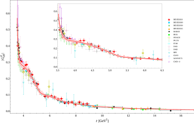
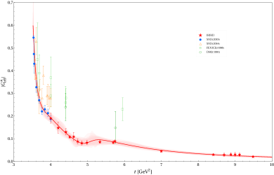
Figure 1: Complete fit to space- and timelike data with bootstrap error (shaded band) compared to data for $|G_{\rm eff}|$ of the proton (upper panel) and neutron (lower panel). Fitted data are depicted by closed symbols; data given by open symbols are shown for comparison only (see Methods for explicit references).

The prominent oscillations in $|G_{\rm eff}|$ between the threshold at $t=4m^{2}$ and $t\approx 6$ GeV² are reproduced by the effective broad poles above threshold. These poles also generate the imaginary part of the form factors in the physical region. Alternatively, these structures can also be generated by including contributions from triangle diagrams with $\Delta\bar{\Delta}$ and $(\Delta\bar{N}+{\rm h.c.})$ intermediate states, see, e.g., Ref. [36]. In principle, these contributions are fixed. However, the corresponding coupling constants are poorly known and a perturbative treatment of these contributions is questionable. For further discussion, see Ref. [37].

The quality of the fit to the spacelike data is comparable to our previous fits of spacelike data only [15, 16]. We obtain $\chi^{2}/{\rm d.o.f}=1.223$ for the full data set, $\chi^{2}/{\rm d.o.f}=1.063$ for the timelike data, and $\chi^{2}/{\rm d.o.f}=1.297$ for the spacelike data. Thus it is warranted to extract the nucleon radii from our combined fit, which has a larger data base than spacelike only fits. We obtain the radii

$$r_{E}^{p} = 0.840^{+0.003}_{-0.002}{}^{+0.002}_{-0.002}\,{\rm fm},$$

$$r_{M}^{p} = 0.849^{+0.003}_{-0.003}{}^{+0.001}_{-0.004}~{}{\rm fm},$$

$$r_{M}^{n} = 0.864^{+0.004}_{-0.004}{}^{+0.006}_{-0.001}~{}{\rm fm},$$ (5)

where the first error is statistical (based on the bootstrap procedure explained in Methods) and the second one is systematic (based on the variations in the spectral functions, see Methods). These values are in good agreement with previous high-precision analyses of spacelike data alone [15, 16] and have comparable errors. For the Zemach radius $r_{z}$ and the third Zemach moment $\langle r^{3}\rangle_{(2)}$ (see Methods), we obtain

$$r_{z} = 1.054^{+0.003}_{-0.002}{}^{+0.000}_{-0.001}\,{\rm fm},$$

$$\langle r^{3}\rangle_{(2)} = 2.310^{+0.022}_{-0.018}{}^{+0.014}_{-0.015}~{}{\rm fm}^{3}.$$ (6)

These values are in good agreement with Lamb shift and hyperfine splittings in muonic hydrogen [38].

Another interesting question in the spacelike region concerns the behavior of the form factor ratio $\mu_{p}G_{E}^{p}/G_{M}^{p}$ for intermediate momentum transfer. Some measurements suggest a zero crossing of this ratio around $t\approx-10$ GeV² [39]. In Fig. 2, we compare our fit to the experimental data for $\mu_{p}G_{E}^{p}/G_{M}^{p}$.

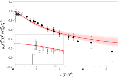
Figure 2: Complete fit to space- and timelike data with bootstrap error (shaded band) compared to JLab data for $\mu_{p}G_{E}^{p}/G_{M}^{p}$ at spacelike momentum transfer. Fitted data are depicted by closed symbols. The data for $|t|<1$ GeV² (open symbols, see also the inset) are shown for comparison only. For references to the data, see Methods.

While we obtain a good description of the data, a zero crossing is disfavored by the combined analysis of space- and timelike data. Thus, data at higher momentum transfer than shown in the figure are required to settle this issue. We further remark that as in the earlier fits to the spacelike data only, the onset of perturbative QCD barely sets in at the highest momentum transfers probed.

Based on quark counting rules [33], the form factor ratio $|G^{p}_{\rm eff}(t)/G^{n}_{\rm eff}(t)|$ should approach a constant as $t\to\infty$ in the timelike region. We show our result for this ratio in Fig. 3. The form factor ratio is constant above $t\simeq 6\,$GeV² and slightly larger than one, with sizeable uncertainties for $t>10$ GeV². However, drawing a clear conclusion about the onset of pQCD certainly requires the separated form factors $G_{E}$ and $G_{M}$, and not just the effective form factor.

Figure 3: Form factor ratio $|G^{p}_{\rm eff}(t)/G^{n}_{\rm eff}(t)|$ in the timelike region for the best fit with the bootstrap uncertainties indicated by the shaded band.

In addition to $|G_{\rm eff}|$, there are also data on the ratio $\lvert G_{E}/G_{M}\rvert$ and on differential cross sections for the proton in the timelike region. The differential cross sections from BESIII in the lowest energy bin ($t\in[1.877,1.950]$ GeV²) are included in our fit and well described. The corresponding differential cross section from BaBar are also well described, when normalized to the total cross section. In Fig. 4, we compare the fit to the proton data for $\lvert G_{E}/G_{M}\rvert$ and give our prediction for the phase of $G_{E}/G_{M}$. We fit only to the BaBar data for $\lvert G_{E}/G_{M}\rvert$ since the BESIII data have much larger error bars.

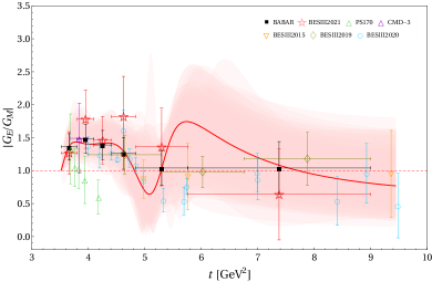
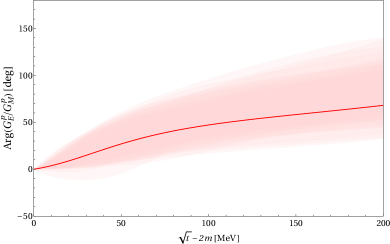
Figure 4: Complete fit to space- and timelike data with bootstrap error (shaded band) compared to proton data for $\lvert G_{E}/G_{M}\rvert$ (closed symbols: fitted, open symbols: not fitted) (upper panel) and our prediction for $\arg(G_{E}/G_{M})$ (lower panel).

The modulus $\lvert G_{E}/G_{M}\rvert$ is well described by our fit but the bootstrap errors grow to more than 100% at $t\approx 6$ GeV². The phase $\arg(G_{E}/G_{M})$ is experimentally unrestricted due to the lack of data and thus has large errors. For energies $\sqrt{t}-2m$ larger than 200 MeV it is essentially unconstrained by our fit. Future measurements of the phase such as planned with PANDA at FAIR would be highly valuable to improve this situation [40].

In summary, for the first time a consistent picture of the nucleons electromagnetic structure based on all spacelike and timelike data from electron scattering and electron-positron annihilation (and its reversed process) emerges. In particular, the extracted proton charge radius $r_{E}^{p}=0.840\,$fm is small and consistent with earlier dispersive analyses [16] and most recent determinations from electron-proton scattering as well as the Lamb shift in electronic and muonic hydrogen (as listed e.g. in Ref. [18]). The Zemach radius and third moment are in agreement with Lamb shift measurements and hyperfine splittings in muonic hydrogen [38]. Still, there are open questions related to the onset of pQCD, the behaviour of the form factor ratio $\mu_{p}G_{E}^{p}/G_{M}^{p}$ at intermediate $|t|$ in the spacelike region, as well as the precise behaviour of this complex-valued ratio in the timelike region. These issues can only be settled by accurate measurements combined with precise analyses as in the framework utilized here.

Appendix A Methods

A.1 Definitions

The matrix element of the electromagnetic (em) current operator $j_{\mu}^{\rm em}$ in the nucleon can be parametrized as

$$\langle N(p^{\prime})|j_{\mu}^{\rm em}|N(p)\rangle=\bar{u}(p^{\prime})\left[F_{1}(t)\gamma_{\mu}+i\frac{F_{2}(t)}{2m}\sigma_{\mu\nu}q^{\nu}\right]u(p)\,,$$ (7)

where $t=(p^{\prime}-p)^{2}<0$ is the four-momentum transfer. The Dirac and Pauli form factors $F_{1}$ and $F_{2}$ are normalized at $t=0$ to the total charge and anomalous magnetic moment, respectively: $F_{1}^{p}(0)=1,\;F_{1}^{n}(0)=0,\;F_{2}^{p}(0)=\kappa_{p}=1.793,$ and $F_{2}^{n}(0)=\kappa_{n}=-1.913$. For the dispersion analysis, it is convenient to decompose the form factors into isoscalar and isovector parts,

$$F_{i}^{s/v}=\frac{1}{2}(F_{i}^{p}\pm F_{i}^{n})\,,\quad i=1,2\,,$$ (8)

since the intermediate states in Eq. (2) have good isospin. The so-called Sachs form factors

$$G_{E}(t)=F_{1}(t)+\frac{t}{4m^{2}}F_{2}(t)\,,\quad G_{M}(t)=F_{1}(t)+F_{2}(t)\,,$$

have a more transparent physical interpretation as Fourier transforms of the charge and magnetization distributions in the Breit frame, respectively.

The low-$t$ behavior of the form factors contains information about the nucleon’s size as seen by an electromagnetic probe. The root mean square radii (loosely called nucleon radii) with $r\equiv\sqrt{\langle r^{2}\rangle}$ are defined via

$$F(t)=F(0)\left[1+t\frac{\langle r^{2}\rangle}{6}+\ldots\right]\,,$$ (9)

where $F(t)$ is a generic form factor. In the case of the electric and Dirac form factors of the neutron, $G_{E}^{n}$ and $F_{1}^{n}$, the expansion starts with the term linear in $t$ and the normalization factor $F(0)$ is dropped.

The Zemach radius $r_{z}$ and third Zemach moment $\left\langle r^{3}\right\rangle_{(2)}$ are defined as

$$r_{z} =\frac{2}{\pi}\int_{-\infty}^{0}\frac{dt}{t\sqrt{-t}}\left(\frac{G_{E}(t)G_{M}(t)}{1+\kappa_{p}}-1\right)~{},$$ (10)

$$\left\langle r^{3}\right\rangle_{(2)} =\frac{24}{\pi}\int_{-\infty}^{0}\frac{dt}{t^{2}\sqrt{-t}}\left(G^{2}_{E}(t)-1-\frac{t}{3}\left\langle r^{2}\right\rangle_{p}\right)~{}.$$ (11)

A.2 Spectral functions

The spectral function applied in our fits has the following structure:

$${\rm Im}\,F_{i}^{s}(t) = {\rm Im}\,F_{i}^{(s,K\bar{K})}(t)+{\rm Im}\,F_{i}^{(s,\rho\pi)}(t)$$ (12)

$$+ \sum_{V=\omega,\phi,s_{1},...}\pi a_{i}^{V}\delta(M^{2}_{V}-t)$$

$$+ \sum_{V=r_{s1},...}\pi a_{i}^{V}\delta(M^{2}_{V}-iM_{V}\Gamma_{V}-t)\,,$$

$${\rm Im}\,F_{i}^{v}(t) = {\rm Im}\,F_{i}^{(v,2\pi)}(t)+\sum_{V=v_{1},...}\pi a_{i}^{V}\delta(M^{2}_{V}-t)$$ (13)

$$+ \sum_{V=r_{v1},...}\pi a_{i}^{V}\delta(M^{2}_{V}-iM_{V}\Gamma_{V}-t)\,,$$

where $i=1,2\,$. It consists of the physical $\omega$ and $\phi$ poles, which have fixed masses, and both narrow and broad effective vector meson poles. The masses of all effective poles and the widths of the broad poles are fitted to the data. Moreover, all vector meson coupling constants are fitted. The $2\pi$, $K\bar{K}$ and $\rho\pi$ continua are determined from other processes and enter as fixed contributions, see Ref. [16] for details. Our best fit consists of $5$ narrow poles in the isoscalar channel $(s)$ and 5 narrow poles in the isovector channel $(v)$ below the nucleon-nucleon threshold and $3s+3v$ broad poles above the threshold. In addition, there are 33 normalization constants for the MAMI and PRad data in the spacelike region. These are discussed in detail in Ref. [16]. In total this adds up to 85 parameters. Including the 11 constraints, namely the 4 for the normalizations of $F_{i}^{p/n}(0)$, 6 for the superconvergence relations and 1 for the fixed neutron charge radius squared, this results in 74 free fit parameters. The vector meson parameters of our best fit are listed in Table 2.

$V_{s}$	$M_{V}$	$\Gamma_{V}$	$a_{1}^{V}$	$a_{2}^{V}$
$\omega$	$0.783$	$0$	$0.701$	$0.338$
$\phi$	$1.019$	$0$	$-0.526$	$-0.997$
$s_{1}$	$1.031$	$0$	$0.422$	$-2.827$
$s_{2}$	$1.120$	$0$	$0.122$	$3.655$
$s_{3}$	$1.827$	$0$	$0.955$	$-1.122$
$r_{s1}$	$1.903$	$0.973$	$-2.653$	$-1.753$
$r_{s2}$	$1.914$	$0.541$	$-3.069$	$2.017$
$r_{s3}$	$1.879$	$0.895$	$4.953$	$0.501$
$V_{v}$	$M_{V}$	$\Gamma_{V}$	$a_{1}^{V}$	$a_{2}^{V}$
$v_{1}$	$1.050$	$0$	$0.782$	$-0.132$
$v_{2}$	$1.323$	$0$	$-4.873$	$-0.645$
$v_{3}$	$1.368$	$0$	$3.518$	$-0.987$
$v_{4}$	$1.462$	$0$	$2.243$	$-3.813$
$v_{5}$	$1.532$	$0$	$-1.422$	$3.668$
$r_{v1}$	$2.256$	$0.239$	$2.552$	$-1.217$
$r_{v2}$	$2.253$	$0.245$	$-1.947$	$0.551$
$r_{v3}$	$2.220$	$0.362$	$-0.985$	$1.061$

Table 2: Parameters for best fit to space- and timelike data. Masses ($M_{V}$) and width ($\Gamma_{V}$) are in GeV while the residua $a_{1,2}^{V}$ are given in GeV². The broad poles are denoted by the symbol $r$.

A.3 Data basis

The data set in the spacelike region is the same as in Ref. [16]. In the timelike region, we include the data sets listed in Table 3.

Data type	Reference
$G_{\rm eff}^{p}$	BESIII2021 [21], BESIII2020 [41], BESIII2019 [42]
	BESIII2015 [43], BABAR [20], E835 [44, 45]
	FENICE [46, 47, 48], PS170 [35], E760 [49]
	DM1 [50], DM2 [51, 52], BES [53]
	CLEO [54], ADONE73 [55], CMD-3 [56]
$G_{\rm eff}^{n}$	BESIII [57], SND2019 [58], SND2014 [59]
	FENICE1998 [48], DM2(1991) [60]
$\lvert G_{E}/G_{M}\rvert$	BABAR [20], BESIII2021 [21], PS170 [35]
	CMD-3 [56], BESIII2015 [43], BESIII2019 [42]
	BESIII2020 [41]

Table 3: Data sets and references for timelike form factors.

A.4 Fitting procedure

The quality of the fits is measured by means of two different $\chi^{2}$ functions, $\chi^{2}_{1}$ and $\chi^{2}_{2}$, which are defined as

$$\chi^{2}_{1} =\sum_{i}\sum_{k}\frac{(n_{k}C_{i}-C(t_{i},\theta_{i},\vec{p}\,))^{2}}{(\sigma_{i}+\nu_{i})^{2}}~{},$$ (14)

$$\chi^{2}_{2} =\sum_{i,j}\sum_{k}(n_{k}C_{i}-C(t_{i},\theta_{i},\vec{p}\,))[V^{-1}]_{ij}$$

$$\qquad\qquad\times(n_{k}C_{j}-C(t_{j},\theta_{j},\vec{p}\,))~{},$$ (15)

where $C_{i}$ are the experimental data at the points $t_{i},\theta_{i}$ and $C(t_{i},\theta_{i},\vec{p}\,)$ are the theoretical value for a given FF parametrization for the parameter values contained in $\vec{p}$. For total cross sections and form factor data the dependence on $\theta_{i}$ is dropped. Moreover, the $n_{k}$ are normalization coefficients for the various data sets (labeled by the integer $k$ and only used in the fits to the differential cross section data in the spacelike region), while $\sigma_{i}$ and $\nu_{i}$ are their statistical and systematical errors, respectively. The covariance matrix $V_{ij}=\sigma_{i}\sigma_{j}\delta_{ij}+\nu_{i}\nu_{j}$. $\chi^{2}_{2}$ is used for those experimental data where statistical and systematical errors are given separately, otherwise $\chi^{2}_{1}$ is adopted. Furthermore, the $\chi^{2}$ of each data set is normalized by the number of data points in order to weight the various data sets without bias.

As done in Ref. [15, 16] the various constraints on the form factors are imposed in a soft way, that is, all constraints are implemented as additive terms to the total $\chi^{2}$ in the following form

$$\chi^{2}_{\rm add.}=p\,[x-\langle x\rangle]^{2}\,\exp\left(p\,[x-\langle x\rangle]^{2}\right)~{},$$ (16)

where $\langle x\rangle$ is the desired value and $p$ is a strength parameter, which regulates the steepness of the exponential well and helps to stabilize the fits. The fits are performed with MINUIT [61] in Fortran.

A.5 Error estimates

The errors from the fits will be quantified using the bootstrap method. We simulate a large number of data sets by randomly varying the points in the original set within the given errors assuming their normal distribution. We then fit to each of them separately, derive the form factor from each fit, and analyze the distribution of these values to generate the error bands for the form factors and the errors of the extracted radii. The theoretical errors are estimated by varying the number of effective vector meson poles. The first error thus gives the uncertainty due to the fitting procedure (bootstrap) and the data while the second one reflects the accuracy of the spectral functions underlying the dispersion-theoretical analysis. Note that these two errors are not in a strict one-to-one correspondence to the commonly given statistical and systematic errors.

References

- [1] K. G. Wilson, Phys. Rev. D 10, 2445 (1974)
- [2] F. Wilczek, Centr. Eur. J. Phys. 10, 1021 (2012) [arXiv:1206.7114 [hep-ph]].
- [3] A. Denig and G. Salme, Prog. Part. Nucl. Phys. 68, 113-157 (2013) [arXiv:1210.4689 [hep-ex]].
- [4] S. Pacetti, R. Baldini Ferroli and E. Tomasi-Gustafsson, Phys. Rept. 550-551, 1-103 (2015).
- [5] V. Punjabi, C. F. Perdrisat, M. K. Jones, E. J. Brash and C. E. Carlson, Eur. Phys. J. A 51, 79 (2015) [arXiv:1503.01452 [nucl-ex]].
- [6] R. Pohl et al., Nature 466, 213 (2010).
- [7] A. Beyer et al., Science 358, 79 (2017).
- [8] H. Fleurbaey et al., Phys. Rev. Lett. 120, 183001 (2018) [arXiv:1801.08816 [physics.atom-ph]].
- [9] N. Bezginov, T. Valdez, M. Horbatsch, A. Marsman, A. C. Vutha and E. A. Hessels, Science 365, 1007 (2019).
- [10] D. S. Armstrong and R. D. McKeown, Ann. Rev. Nucl. Part. Sci. 62, 337-359 (2012) [arXiv:1207.5238 [nucl-ex]].
- [11] F. E. Maas and K. D. Paschke, Prog. Part. Nucl. Phys. 95, 209-244 (2017).
- [12] S. Bacca and S. Pastore, J. Phys. G 41, no.12, 123002 (2014) [arXiv:1407.3490 [nucl-th]].
- [13] D. R. Phillips, Ann. Rev. Nucl. Part. Sci. 66, 421-447 (2016).
- [14] H. Krebs, Eur. Phys. J. A 56, no.9, 234 (2020) [arXiv:2008.00974 [nucl-th]].
- [15] Y. H. Lin, H.-W. Hammer and U.-G. Meißner, Phys. Lett. B 816, 136254 (2021) [arXiv:2102.11642 [hep-ph]].
- [16] Y. H. Lin, H.-W. Hammer and U.-G. Meißner, Eur. Phys. J. A 57, 255 (2021) [arXiv:2106.06357 [hep-ph]].
- [17] J. C. Bernauer and R. Pohl, Sci. Am. 310, no.2, 18-25 (2014)
- [18] H.-W. Hammer and U.-G. Meißner, Sci. Bull. 65, 257-258 (2020) [arXiv:1912.03881 [hep-ph]].
- [19] J. P. Karr, D. Marchand and E. Voutier, Nature Rev. Phys. 2, no.11, 601-614 (2020).
- [20] J. P. Lees et al. [BaBar], Phys. Rev. D 87, no.9, 092005 (2013) [arXiv:1302.0055 [hep-ex]].
- [21] M. Ablikim et al. [BESIII], Phys. Lett. B 817, 136328 (2021) [arXiv:2102.10337 [hep-ex]].
- [22] G. F. Chew, R. Karplus, S. Gasiorowicz and F. Zachariasen, Phys. Rev. 110, no.1, 265 (1958).
- [23] P. Federbush, M. L. Goldberger and S. B. Treiman, Phys. Rev. 112, 642-665 (1958).
- [24] W. R. Frazer and J. R. Fulco, Phys. Rev. 117, 1609-1614 (1960)
- [25] M. Hoferichter, B. Kubis, J. Ruiz de Elvira, H.-W. Hammer and U.-G. Meißner, Eur. Phys. J. A 52, no.11, 331 (2016) [arXiv:1609.06722 [hep-ph]].
- [26] M. Hoferichter, J. Ruiz de Elvira, B. Kubis and U.-G. Meißner, Phys. Rept. 625, 1-88 (2016) [arXiv:1510.06039 [hep-ph]].
- [27] V. Bernard, N. Kaiser and U.-G. Meißner, Nucl. Phys. A 611, 429-441 (1996) [arXiv:hep-ph/9607428 [hep-ph]].
- [28] N. Kaiser and E. Passemar, Eur. Phys. J. A 55, no.2, 16 (2019) [arXiv:1901.02865 [nucl-th]].
- [29] H.-W. Hammer and M.J. Ramsey-Musolf, Phys. Rev. C 60, 045205 (1999) [Erratum-ibid. C 62, 049903 (2000)] [arXiv:hep-ph/9812261].
- [30] H.-W. Hammer and M.J. Ramsey-Musolf, Phys. Rev. C 60, 045204 (1999) [Erratum-ibid. C 62, 049902 (2000)] [arXiv:hep-ph/9903367].
- [31] U.-G. Meißner, V. Mull, J. Speth and J. W. van Orden, Phys. Lett. B 408, 381 (1997) [arXiv:hep-ph/9701296].
- [32] I. Sabba Stefanescu, J. Math. Phys. 21, 175 (1980).
- [33] G. P. Lepage and S. J. Brodsky, Phys. Rev. D 22, 2157 (1980).
- [34] A. A. Filin, D. Möller, V. Baru, E. Epelbaum, H. Krebs and P. Reinert, Phys. Rev. C 103 (2021) no.2, 024313 [arXiv:2009.08911 [nucl-th]].
- [35] G. Bardin, et al. Nucl. Phys. B 411, 3-32 (1994).
- [36] I. T. Lorenz, H.-W. Hammer and U.-G. Meißner, Phys. Rev. D 92, no.3, 034018 (2015) [arXiv:1506.02282 [hep-ph]].
- [37] A. Bianconi and E. Tomasi-Gustafsson, Phys. Rev. Lett. 114, no.23, 232301 (2015) [arXiv:1503.02140 [nucl-th]].
- [38] A. Antognini, F. Nez, K. Schuhmann, F. D. Amaro, FrancoisBiraben, J. M. R. Cardoso, D. S. Covita, A. Dax, S. Dhawan and M. Diepold, et al. Science 339, 417-420 (2013)
- [39] J. Arrington, K. de Jager and C. F. Perdrisat, J. Phys. Conf. Ser. 299, 012002 (2011) [arXiv:1102.2463 [nucl-ex]].
- [40] A. Dbeyssi [PANDA], EPJ Web Conf. 204, 01004 (2019).
- [41] M. Ablikim et al. [BESIII], Phys. Rev. Lett. 124, no.4, 042001 (2020) [arXiv:1905.09001 [hep-ex]].
- [42] M. Ablikim et al. [BESIII], Phys. Rev. D 99, no.9, 092002 (2019) [arXiv:1902.00665 [hep-ex]].
- [43] M. Ablikim et al. [BESIII], Phys. Rev. D 91, no.11, 112004 (2015) [arXiv:1504.02680 [hep-ex]].
- [44] M. Ambrogiani et al. [E835], Phys. Rev. D 60, 032002 (1999)
- [45] M. Andreotti, S. Bagnasco, W. Baldini, D. Bettoni, G. Borreani, A. Buzzo, R. Calabrese, R. Cester, G. Cibinetto and P. Dalpiaz, et al. Phys. Lett. B 559, 20-25 (2003)
- [46] A. Antonelli, R. Baldini, M. Bertani, M. E. Biagini, V. Bidoli, C. Bini, T. Bressani, R. Calabrese, R. Cardarelli and R. Carlin, et al. Phys. Lett. B 313, 283-287 (1993)
- [47] A. Antonelli, R. Baldini, M. Bertani, M. E. Biagini, V. Bidoli, C. Bini, T. Bressani, R. Calabrese, R. Cardarelli and R. Carlin, et al. Phys. Lett. B 334, 431-434 (1994)
- [48] A. Antonelli, R. Baldini, P. Benasi, M. Bertani, M. E. Biagini, V. Bidoli, C. Bini, T. Bressani, R. Calabrese and R. Cardarelli, et al. Nucl. Phys. B 517, 3-35 (1998)
- [49] T. A. Armstrong et al. [E760], Phys. Rev. Lett. 70, 1212-1215 (1993)
- [50] B. Delcourt, I. Derado, J. L. Bertrand, D. Bisello, J. C. Bizot, J. Buon, A. Cordier, P. Eschstruth, L. Fayard and J. Jeanjean, et al. Phys. Lett. B 86, 395-398 (1979)
- [51] D. Bisello, S. Limentani, M. Nigro, L. Pescara, M. Posocco, P. Sartori, J. E. Augustin, G. Busetto, G. Cosme and F. Couchot, et al. Nucl. Phys. B 224, 379 (1983)
- [52] D. Bisello et al. [DM2], Z. Phys. C 48, 23-28 (1990)
- [53] M. Ablikim et al. [BES], Phys. Lett. B 630, 14-20 (2005) [arXiv:hep-ex/0506059 [hep-ex]].
- [54] T. K. Pedlar et al. [CLEO], Phys. Rev. Lett. 95, 261803 (2005) [arXiv:hep-ex/0510005 [hep-ex]].
- [55] M. Castellano, G. Di Giugno, J. W. Humphrey, E. Sassi Palmieri, G. Troise, U. Troya and S. Vitale, Nuovo Cim. A 14, 1-20 (1973)
- [56] R. R. Akhmetshin et al. [CMD-3], Phys. Lett. B 759, 634-640 (2016) [arXiv:1507.08013 [hep-ex]].
- [57] M. Ablikim et al. [BESIII], [arXiv:2103.12486 [hep-ex]].
- [58] V. P. Druzhinin and S. I. Serednyakov, EPJ Web Conf. 212, 07007 (2019)
- [59] M. N. Achasov, A. Y. Barnyakov, K. I. Beloborodov, A. V. Berdyugin, D. E. Berkaev, A. G. Bogdanchikov, A. A. Botov, T. V. Dimova, V. P. Druzhinin and V. B. Golubev, et al. Phys. Rev. D 90, no.11, 112007 (2014) [arXiv:1410.3188 [hep-ex]].
- [60] M. E. Biagini, E. Pasqualucci and A. Rotondo, Z. Phys. C 52, 631-634 (1991)
- [61] F. James and M. Roos, Comput. Phys. Commun. 10, 343-367 (1975).