On the cross-streamline lift of microswimmers in viscoelastic flows

Abstract

The current work studies the dynamics of a microswimmer in pressure-driven flow of a weakly viscoelastic fluid. Employing the second-order fluid model, we show that the self-propelling swimmer experiences a viscoelastic swimming lift in addition to the well-known passive lift that arises from its resistance to shear flow. Using the reciprocal theorem, we evaluate analytical expressions for the swimming lift experienced by neutral and pusher/puller-type swimmers and show that they depend on the hydrodynamic signature associated with the swimming mechanism. We find that for neutral swimmers focusing towards the centerline is accelerated by two orders of magnitude, while for force-dipole swimmers no net modification in cross-streamline migration occurs.

Biological microswimmers are ubiquitous in polymeric media such as cervical, bronchial, and intestinal mucus films Suarez and Pacey (2006); Levy et al. (2014). During the generation of biofilms, detrimental to bio-engineering and industrial processes, most bacteria release a mixture of proteins, DNA, and polysaccharides, endowing the fluid with viscoelastic properties Persat et al. (2015); Conrad and Poling-Skutvik (2018), which significantly alter the swimmer’s dynamics Jabbarzadeh et al. (2014). Pathogens like ulcer-causing Helicobacter pylori thrive by altering the rheology of mucus lining in stomach Celli et al. (2009). Recent theoretical and experimental studies on the dynamics of motile microorganisms in Newtonian flows have revealed their rich dynamics and ability to swim against fluid flows, which aids in seeking nutrients and in reproduction Bretherton and Rothschild (1961); Hill et al. (2007); Nash et al. (2010); Zöttl and Stark (2012, 2013); Tung et al. (2015); Mathijssen et al. (2019); Lauga (2020).

Although recent works have provided insights in self-propulsion in non-Newtonian environments Lauga (2007); Shen and Arratia (2011); Zhu et al. (2012); Pak et al. (2012); Keim et al. (2012); Elfring and Lauga (2015); Sznitman and Arratia (2015); Li and Ardekani (2015); Datt et al. (2015); Li and Ardekani (2016, 2017); Ives and Morozov (2017); Datt et al. (2017); Zhang et al. (2018); Zöttl and Yeomans (2019); Choudhary et al. (2020a); Binagia et al. (2020); Lauga (2020), few have studied the impact of fluid rheology on the dynamics of microswimmers in confined flows Mathijssen et al. (2016); De Corato and D’Avino (2017); Ardekani and Gore (2012). Mathijssen et al. (2016) developed a model to predict the dynamical states of microswimmers in non-Newtonian Poiseuille flows. Employing a second-order fluid model, they demonstrated that normal-stress differences reorient the swimmers to cause centerline upstream migration (rheotaxis). This suggests that non-Newtonian properties can help microorganisms evade the boundary accumulation, prevalent in quiescent Newtonian fluids Berke et al. (2008); Smith et al. (2009).

The evidence of centerline reorientation of microswimmers can be traced back to pioneering works on viscoelastic focusing of passive particles in Poiseuille flows Karnis and Mason (1966); Gauthier et al. (1971); Ho and Leal (1976). These studies showed that normal stresses exert a lift force that focuses the particles on the centerline. Ho and Leal (1976) used the reciprocal theorem and derived an analytical expression for this lift in weakly elastic Boger fluids. The study suggested that the hydrodynamic disturbances around the particle produces a hoop stress that, in the presence of non-uniform shear rate, generates a cross-streamline lift. Recent progress in electrophoresis Li and Xuan (2018); Choudhary et al. (2020b, 2021) has also shed light on the importance of hydrodynamic disturbances in determining these lift forces.

Active microswimmers, as opposed to passive particles, generate additional disturbance flow fields in the fluid due to their self-propulsion. Therefore, the associated lift force or velocity should also have an active component that is characteristic of the self-propulsion mechanism. Since this component is absent in the recently proposed models Mathijssen et al. (2016), in this communication we derive the ‘swimming lift’ in a second-order fluid (SOF), and show how it affects the dynamics of a microswimmer in the Poiseuille flow of a viscoelastic fluid. We choose the SOF model because it provides an asymptotic approximation for a majority of slow and slowly varying viscoelastic flows Leal (1979); Bird et al. (1987).

Figure 1 shows a spherical swimmer of radius $a$ at position $\bm{r}$ that self-propels with velocity $\bm{v}_{s}=v_{s}\bm{p}$ in a two-dimensional pressure-driven flow $\bm{v}_{f}=v_{m}[1-({x}/{w})^{2}]\,\bm{e}_{z}$, where $v_{m}$ is the maximum flow velocity and $w$ is the half channel width. The flow profile of the second-order fluid is identical to Poiseuille flow but the pressure field varies in $x-$direction Ho and Leal (1976). In the absence of noise, the swimmer’s dynamics is governed by

$$\bm{\dot{r}}=\bm{p}+\bar{\bm{v}}_{f}+\mathcal{F}(x,{\bm{p}})\,\bm{e}_{x}\,,\quad\bm{\dot{p}}=\frac{1}{2}\left(\nabla\times\bar{\bm{v}}_{f}\right)\times\bm{p},$$ (1)

where the velocities are non-dimensionalized by swimming speed $v_{s}$, lengths by $w$, and time by $w/v_{s}$. $\mathcal{F}$ denotes the total viscoelastic lift velocity, which comprises the passive and swimming lift. Below, we derive the analytical expressions for the lift velocities. We note that normal stresses also modify the particle rotation and the drift velocity along the channel axis. We evaluated these modifications and found that they do not play a significant role in determining the swimmer dynamics.

The inertia-less or creeping flow hydrodynamics is governed by the continuity equations for mass and momentum, which we formulate here in the co-moving swimmer frame $\{\tilde{x},\tilde{y},\tilde{z}\}$ as:

$$\tilde{\nabla}\cdot\bm{V}=0,\;\tilde{\nabla}\cdot\bm{\mathsf{T}}=0$$ (2)

in order to calculate the viscoelastic lift velocity. Length, velocity, and pressure in (2) are non-dimensionalized by $a$, $\kappa v_{m}$, and $\mu\kappa v_{m}/a$, respectively. Here, $\kappa$ is the particle to channel width ratio ($a/2w$) and $\mu$ is the fluid viscosity. In the above equation, $\bm{\mathsf{T}}$ is the total stress tensor of a second-order fluid and thus has the form Bird et al. (1987): $\bm{\mathsf{T}}=-P\,\bm{\mathsf{I}}+2\,\bm{\mathsf{E}}+\text{Wi}\,\bm{\mathsf{S}}$. Here, $\bm{\mathsf{E}}$ denotes the rate of strain tensor and $\text{Wi}=(\Psi_{1}+\Psi_{2})G/\mu$ is the shear based Weissenberg number, where $\mu$ is the viscosity, $G=v_{m}/2w$ characterizes the shear rate in the background flow, and $\Psi_{1},\Psi_{2}$ represent the dimensional steady-shear normal stress coefficients that are measured experimentally Bird et al. (1987). The polymeric stress tensor $\bm{\mathsf{S}}=4\bm{\mathsf{E}}\cdot\bm{\mathsf{E}}+2\delta\overset{\Delta}{\bm{\mathsf{E}}}$ is non-linear in $\bm{\mathsf{E}}$ and contains the lower-convected time derivative of $\bm{\mathsf{E}}$ denoted by $\Delta$. The viscometric parameter $\delta=-\Psi_{1}/2(\Psi_{1}+\Psi_{2})$ generally varies from $-0.5$ to $-0.7$ for most viscoelastic fluids Caswell and Schwarz (1962); Leal (1975); Koch and Subramanian (2006).

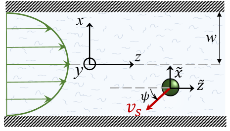
Figure 1: A spherical microswimmer with velocity $v_{s}\bm{p}$ moves in a pressure-driven flow of a second-order fluid inside a channel with half width $w$. The coordinate frame $\{\tilde{x},\tilde{y},\tilde{z}\}$ co-moves with the swimmer.

We now focus on determining the lift velocity of a microswimmer that disturbs the background flow in two ways. First of all, the microswimmer resists straining by the flow and second, it generates a flow field characteristic of its swimming mechanism, for which we first take a source-dipole swimmer. We split the full velocity field ($\bm{V}=\bm{v}^{\infty}+\bm{v}$) into background flow field $\bm{v}^{\infty}$ and disturbance field $\bm{v}$. Substituting this in the governing equations (2) yields:

$$\tilde{\nabla}\cdot\bm{v}=0,\quad-\tilde{\nabla}p+\tilde{\nabla}^{2}\bm{v}=-\text{Wi}(\tilde{\nabla}\cdot\bm{\mathsf{s}}),$$ (3)

where $\bm{\mathsf{s}}$ is the polymeric stress tensor associated with the disturbance flow field (elaborated in the electronic supplementary material ESI). Assuming weak viscoelasticity, we perform a perturbation expansion in Wi and divide Eq. (3) into two problems: the Stokes equation for the zeroth order of the disturbance field and $-\tilde{\nabla}p_{1}+\tilde{\nabla}^{2}\bm{v}_{1}=-\tilde{\nabla}\cdot\bm{\mathsf{s}}_{0}$ at first order. Following earlier works on viscoelastic lift Ho and Leal (1976); Choudhary et al. (2020b), we use the reciprocal theorem to attain the lift velocity from the first-order problem

$$\mathcal{F}=-\frac{\text{Wi}}{6\pi}\int_{V_{f}}\bm{\mathsf{s}}_{0}:\tilde{\nabla}\bm{u}^{t}\,\text{d}V.$$ (4)

Here, $\bm{u}^{t}$ is the auxiliary or test velocity field that belongs to a forced particle moving along the $x$-direction with unit velocity in a Newtonian fluid. The polymeric stress $\bm{\mathsf{s}}_{0}$ corresponds to the Stokes solution $\bm{v}_{0}$ of the microswimmer consisting of (i) a source-dipole field, which we attain from the squirmer model Lighthill (1952); Blake (1971a); Zöttl and Stark (2016), $\bm{v}_{0}^{\text{swim}}=\frac{v_{s}\bm{p}}{2\tilde{r}^{3}}\bm{\cdot}\left[\frac{3\tilde{\bm{r}}\tilde{\bm{r}}}{\tilde{r}^{2}}-\bm{\mathsf{I}}\right]$, and (ii) the passive disturbance field $\bm{v}_{0}^{\text{passive}}$, which is led by the stresslet; higher order terms are obtained from Lamb’s general solution Lamb (1975). Using the corresponding $\bm{\mathsf{s}}_{0}$ in Eq. (4), results in the viscoelastic lift velocity given in units of $v_{s}$:

$$\mathcal{F}(x,\psi)=\text{Wi}\left[\frac{80}{9}x\,\bar{v}_{m}\kappa^{2}(1+3\delta)-x\,(1+\delta)\cos\psi\right].$$ (5)

The first component in Eq. (5) is the passive lift $\mathcal{F}_{\text{passive}}$ Ho and Leal (1976). By fixing $\delta$ to a widely-used value of $-0.5$ (i.e. $\Psi_{2}=0$), we observe that $\mathcal{F}_{\text{passive}}$ focuses the particle towards the centerline. The second component is the swimming lift $\mathcal{F}_{swim}$ that arises due to the source-dipole disturbance created by the neutral swimmer. We note two striking features of $\mathcal{F}_{\text{swim}}$: the dependence on swimmer orientation through $\cos\psi$ and that its magnitude is larger by a factor $\kappa^{-2}$ compared to the first term.

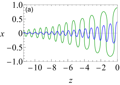
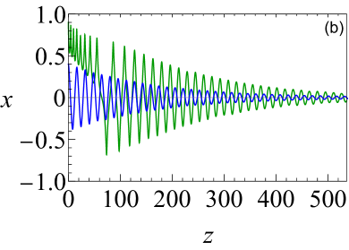
Figure 2: Trajectories showing the centerline focusing of a neutral (source-dipole) swimmer oriented upstream while (a) swimming upstream ($\bar{v}_{m}=0.9$) and (b) drifting downstream ($\bar{v}_{m}=8$). Other parameters: $\text{Wi}=0.1,\,\kappa=0.1,\,\delta=-0.5.$ The blue and green trajectories only differ in the initial condition $x_{0}$.

Now, we substitute $\mathcal{F}$ into the dynamic equations (1) and examine the effect of $\mathcal{F}_{\text{swim}}$ on the microswimmer dynamics. We find two fixed points in the $x-\psi$ plane at $x=0$, with the microswimmer oriented upstream ($\psi=0$) or downstream ($\psi=\pm\pi$). A linear stability analysis provides the following eigenvalues for these fixed points:

$$\lambda_{1}\approx \frac{\text{Wi}}{18}\left[-9(1+\delta)+80(1+3\delta)\kappa^{2}\bar{v}_{m}\right]\pm{\rm i}\,\bar{v}_{m}^{1/2},$$

$$\lambda_{2}\approx \frac{\text{Wi}}{18}\left[9(1+\delta)+80(1+3\delta)\kappa^{2}\bar{v}_{m}\right]\pm\,\bar{v}_{m}^{1/2}.$$ (6)

For a typical value of $\delta=-0.5$ and weak viscoelasticity limit (${\rm Wi}\ll 1$), the downstream swimming corresponds to a saddle fixed point ($\lambda_{2}$), while the upstream swimming along $x=0$ corresponds to a stable fixed point ($\lambda_{1}$). For $\delta=-0.5$, the sign of the real part of $\lambda_{1}$ shows that both swimming and passive lift components stabilize the upstream swimming. However, the strong swimming lift can help the neutral microswimmer attain centerline equilibrium more rapidly by a relaxation factor of $\kappa^{-2}$, as also shown in the trajectories of Fig.2 that are evaluated by substituting (5) in (1).

Now, we shift our attention from neutral squirmers to flagellated microorganisms, such as E. coli and Chlamydomonas, that generate a force-dipole field at the leading order Pedley and Kessler (1992); Berke et al. (2008): $\bm{v}_{0}=\mathcal{P}\bm{r}\big{[}\frac{-1}{r^{3}}+3\frac{\left(\bm{r}\cdot\bm{p}\right)^{2}}{r^{5}}\big{]}$. Here $\mathcal{P}$ is the force-dipole strength in units of $8\pi\mu a^{2}v_{s}$, which depends on the swimming mechanism Berke et al. (2008); Drescher et al. (2010, 2011). Earlier studies on E. coli Drescher et al. (2011); Chattopadhyay et al. (2006) and Chlamydomonas Minoura and Kamiya (1995) suggest that $|\mathcal{P}|$ varies roughly between 0.04 - 0.3. Following the procedure outlined for a source-dipole swimmer, we obtain the swimming lift velocity of the force-dipole swimmer as

$$\mathcal{F}_{\text{swim}}=(8/3)\text{Wi}\,\kappa\,\mathcal{P}(1+3\delta)\sin 2\psi,$$ (7)

and find it to depend on the constant curvature in Poiseuille flow, as detailed in ESI. Although this lift is larger than $\mathcal{F}_{\text{passive}}$ by a factor $\kappa^{-1}$, there is no net lateral motion because the pure angular dependence cancels out on average as the particle tumbles continuously. The trajectories in Fig.3 (a) and (b) show the dynamics of a force-dipole swimmer; the focusing along the centerline is purely due to $\mathcal{F}_{\text{passive}}$.

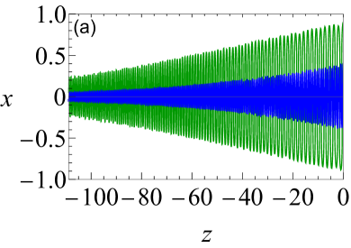
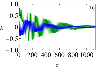
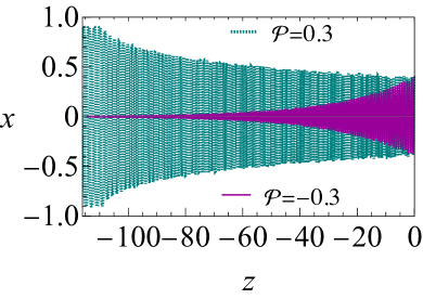
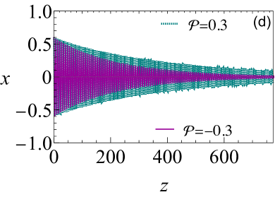
Figure 3: Trajectories showing the centerline focusing of pusher/puller in (a) upstream swimming ($\bar{v}_{m}=0.9$) and (b) downstream drifting ($\bar{v}_{m}=8$). (c) Upstream ($\bar{v}_{m}=0.9$) and (d) downstream trajectories ($\bar{v}_{m}=3$) with hydrodynamic wall interactions (On the cross-streamline lift of microswimmers in viscoelastic flows) incorporated. We employ hard-core repulsion at the walls. Other parameters: $\text{Wi}=0.1,\,\kappa=0.1,\,\delta=-0.5.$

So far we have neglected the hydrodynamic interactions of microswimmers with the bounding channel walls. For force-dipole swimmers, the hydrodynamic wall interactions add a modification of order $\kappa^{2}$ and $\kappa^{3}$ to the evolution equations of position and orientation, respectively Zöttl and Stark (2012); Spagnolie and Lauga (2012):

$$\dot{x} =-\sin\psi+\mathcal{F}-\frac{3\mathcal{P}(3\sin^{2}\psi-1)}{8}\kappa^{2}\left[\frac{1}{(1-x)^{2}}-\frac{1}{(1+x)^{2}}\right],$$

$$\dot{\psi} =x\bar{v}_{m}-\frac{3\mathcal{P}\sin 2\psi}{16}\kappa^{3}\left[\frac{1}{(1-x)^{3}}+\frac{1}{(1+x)^{3}}\right].$$ (8)

Upstream trajectories in Fig. 3(c) closely resemble the behavior reported previously for pure Newtonian fluids Zöttl and Stark (2012). We observe that the hydrodynamic wall attraction of pushers Berke et al. (2008) overcomes $\mathcal{F}_{\text{passive}}$ and results in swinging across the whole channel cross section, where the strong vorticity near the walls always re-orients the swimmer away from it. Pullers are repelled from walls Zöttl and Stark (2012) and, therefore, rapidly focus on the centerline. In contrast, for downstream drifting at large flow rates [Fig. 3(d)], $\mathcal{F}_{passive}$ dominates over the hydrodynamic wall interactions and all trajectories tend towards the centerline. We note that for source-dipole swimmers the hydrodynamic wall interactions are an order $\kappa$ weaker, and therefore do not alter the trajectories qualitatively.

In conclusion, the current study analyzes microswimmers in weakly viscoelastic pressure-driven flows. For neutral and pusher/puller microswimmers, we derive an additional swimming lift velocity depending on the swimmer’s hydrodynamic signature that adds to the passive viscoelastic lift Ho and Leal (1976); Lee et al. (2010); Mathijssen et al. (2016); D’Avino et al. (2017). For source-dipole (neutral) swimmers, the swimming lift is two orders of magnitude stronger than the passive lift, which was considered alone in a recent study Mathijssen et al. (2016). The current work shows that the swimming lift accelerates the centerline focusing. For force-dipole swimmers (pusher/puller), the swimming lift does not contribute to a net cross-streamline migration. Incorporating hydrodynamic wall interactions, we show that upstream swimming for weak flow strengths qualitatively follows the behavior in Newtonian fluids Zöttl and Stark (2012): attraction of pushers towards the channel walls and repulsion of pullers. The downstream drifting along the centerline qualitatively remains the same as that of a passive particle.

These results suggest that normal stresses in viscoelastic fluids generated by the microswimmer’s flow field can accelerate the centerline focusing. However, this strongly depends on the hydrodynamic signature of the microswimmer. Even for a weakly viscoelastic fluid ($\text{Wi}=0.1$), we observe rapid focusing within a traveled distance of 10-500 times the channel width (Fig. 2), which amounts to ca. $1-50\text{mm}$ and is quite realistic for microfluidic channels. Thereby, this work contributes to the understanding of swimming in more realistic biological fluids. Furthermore, the current work offers several new directions to explore. For instance, elongated microswimmers perform Jeffery orbits in sheared Newtonian fluids Jeffery (1922). In viscoelastic fluids the flow disturbances from swimming will alter the orientation evolution of these orbits and hence the swimmer dynamics De Corato and D’Avino (2017). Impact of shear-thinning fluids is also an interesting outlook, which can be achieved by the use of more detailed rheological models Bird et al. (1987).

Support from Alexander von Humboldt fellowship is gratefully acknowledged.

I Problem formulation

The schematic in Fig. S1 (a) shows a neutrally buoyant spherical microswimmer suspended in pressure-driven flow of a polymeric fluid between two walls. In order to derive the expressions for the lift velocities, we work in a reference frame that translates with the swimmer ${(\tilde{x},\tilde{y},\tilde{z})}$. For simplicity, we temporarily drop the tilde $\tilde{}$ notation. Fig. S1 (b) shows the non-dimensional description, where $s=d/2w$ and $s/\kappa=d/a$ is the distance from the bottom wall normalized by the particle radius $a$.

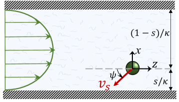
Figure S1: (left) A spherical microswimmer self-propels with velocity $\bm{v}_{s}=v_{s}\bm{p}$ in a planar Poiseuille flow inside a channel with half width $w$. The coordinate frame $\{\tilde{x},\tilde{y},\tilde{z}\}$ co-moves with the swimmer. (right ) Schematic with all lengths normalized by particle radius $a$. The tilde notation of the coordinates is shown to be dropped for brevity.

We split the actual velocity field into the background flow field $\bm{v}^{\infty}$ and the disturbance field $\bm{v}$ (i.e. $\bm{v}_{\text{actual}}=\bm{v}+\bm{v}^{\infty}$), and substitute in Eq. (2) of the article. The inertia-less hydrodynamics of the disturbance field is governed by the continuity and momentum equations in the co-moving swimmer frame $\{\tilde{x},\tilde{y},\tilde{z}\}$ as:

$$\nabla\cdot\bm{v} = 0,\quad-\nabla p+\nabla^{2}\bm{v}=-\text{Wi}\,(\nabla\cdot\bm{\mathsf{s}}),\text{ where}$$

$$\bm{\mathsf{s}} = 4(\bm{\mathsf{e}}\cdot\bm{\mathsf{e}}+\bm{\mathsf{w}})+2\,\delta(\overset{\Delta}{\bm{\mathsf{e}}}+\overset{\Delta}{\bm{\mathsf{w}}}).$$ (S1)

Here, $\bm{\mathsf{e}}$ is the rate of strain tensor for the disturbance flow $(\nabla\bm{v}+\nabla\bm{v}^{\dagger})/2$, whereas $\bm{\mathsf{w}}$, $\overset{\Delta}{\bm{\mathsf{e}}}$ and $\overset{\Delta}{\bm{\mathsf{w}}}$ are the different parts of the perturbation $\bm{\mathsf{s}}$ of the polymeric tensor due to the disturbance flow field $\bm{v}$:

$$\bm{\mathsf{w}} = \bm{\mathsf{e}}^{\infty}\cdot\bm{\mathsf{e}}+\bm{\mathsf{e}}\cdot\bm{\mathsf{e}}^{\infty},$$

$$\overset{\Delta}{\bm{\mathsf{e}}} = \bm{v}\cdot\nabla\bm{\mathsf{e}}+\bm{\mathsf{e}}\cdot\nabla\bm{v}^{\dagger}+\nabla\bm{v}\cdot\bm{\mathsf{e}},$$

$$\overset{\Delta}{\bm{\mathsf{w}}} = {\bm{v}^{\infty}}\cdot\nabla\bm{\mathsf{e}}+\bm{\mathsf{e}}\cdot\nabla{\bm{v}^{\infty}}^{\dagger}+\nabla{\bm{v}^{\infty}}\cdot\bm{\mathsf{e}}+\,\bm{v}\cdot\nabla\bm{\mathsf{e}}^{\infty}$$

$$+\bm{\mathsf{e}}^{\infty}\cdot\nabla\bm{v}^{\dagger}+\nabla\bm{v}\cdot\bm{\mathsf{e}}^{\infty},$$

where $\bm{\mathsf{e}}^{\infty}$ is the rate of strain tensor for the undisturbed flow, $\overset{\Delta}{\bm{\mathsf{e}}}$ is the lower convected derivative of $\bm{\mathsf{e}}$ (also known as the Rivlin-Eriksen tensor), $\bm{\mathsf{w}}$ is the ‘interaction tensor’ (arising from the interaction between background flow and disturbance field), and $\overset{\Delta}{\bm{\mathsf{w}}}$ is its lower convected derivative.

The above equations are non-dimensionalized using $a,\,\kappa v_{m},\,\mu\kappa v_{m}/a$ as the characteristic scales for length, velocity, and pressure, respectively. The definitions of these dimensional parameters $a$ (particle size), $\kappa=a/2w$, and $v_{m}$ (maximum flow velocity) are consistent with the communication article. In our case, $\bm{v}^{\infty}$ is the undisturbed Poiseuille flow velocity in the frame of reference translating with the particle

$${\bm{v}^{\infty}}=\left({\alpha+\beta x+\gamma{x^{2}}}\right){\bm{e}_{z}}-{\bm{U}_{p}},$$ (S3)

where $\bm{U}_{p}$ is the total velocity of the swimmer, i.e., swimming velocity $\bm{v}_{s}$ plus advection due to the Poiseuille flow and the lift velocities. The constants $\alpha,\beta$ and $\gamma$ are:

$$\alpha=4s\left({1-s}\right)/\kappa,\,\beta=4\left({1-2s}\right),\,\gamma=-4{\kappa},$$ (S4)

where $\beta$ and $\gamma$ represent the shear and curvature of the background flow, respectively. The boundary conditions of the disturbance flow field are

$$\bm{v}=\bm{v}_{\theta}+{\bm{\Omega}_{s}}\times\bm{r}-\bm{v}^{\infty}\quad\mbox{at\ }r=1,$$ (S5a)

$$\bm{v}=0\quad\mbox{at walls,\ }$$ (S5b)

$$\bm{v}\rightarrow\bm{0}\quad\mbox{as\ }\{y,z\}\rightarrow\infty.$$ (S5c)

Here, the walls are located at $x=-s/\kappa$ and $x=(1-s)/\kappa$, and $\bm{v}_{\theta}$ represents the prescribed tangential surface velocity of the spherical microswimmer.

II Perturbation expansion

We find the viscoelastic lift or migration velocities at $O(\text{Wi})$ using a regular perturbation expansion. For small values of Wi, the disturbance field variables are expanded as:

$$\xi=\xi_{0}+\text{Wi}\;\xi_{1}+\cdots.$$ (S6)

Here, $\xi$ is a generic field variable which represents velocity ($\bm{v}$), pressure ($p$), translational ($\bm{U}_{p}$) and angular velocity ($\bm{\Omega}_{p}$). We substitute (S6) in the equations governing the disturbance field (I) and obtain the problem at $O(1)$ (i.e. Stokes problem) as

$$\left.\begin{array}[]{l}\quad\;\;\,\quad\nabla\cdot{\bm{v}_{0}}=0,\\ {\nabla^{2}}{\bm{v}_{0}}-\nabla{p_{0}}=\bm{0},\\ \qquad\quad\;\quad{\bm{v}_{0}}=\bm{v}_{\theta}+{\bm{\Omega}_{p0}}\times\bm{r}-{\bm{v}_{0}^{\infty}}\quad\mbox{at\ }r=1,\\ \qquad\quad\;\quad{\bm{v}_{0}}=0\quad\mbox{at walls},\\ \qquad\quad\;\quad{\bm{v}_{0}}\to\bm{0}\quad\mbox{as\ }\{y,z\}\rightarrow\infty.\end{array}\right\}$$ (S7)

and at $O(\text{Wi})$ as:

$$\left.\begin{array}[]{l}\qquad\;\quad\nabla\cdot{\bm{v}_{1}}=0,\\ \;\,\,{\nabla^{2}}{\bm{v}_{1}}-\nabla{p_{1}}=-\nabla\cdot\bm{\mathsf{s}}_{0},\\ \qquad\qquad\quad{\bm{v}_{1}}={\bm{U}_{p1}}+{\bm{\Omega}_{p1}}\times\bm{r}\quad\mbox{at\ }r=1,\\ \qquad\qquad\quad{\bm{v}_{1}}=\bm{0}\quad\mbox{at walls},\\ \qquad\qquad\quad{\bm{v}_{1}}\to\bm{0}\quad\mbox{as\ }\{y,z\}\rightarrow\infty.\end{array}\right\}$$ (S8)

In (S7), $\bm{v}^{\infty}_{0}=\left({\alpha+\beta x+\gamma{x^{2}}}\right){\bm{e}_{z}}-{\bm{U}_{p\,0}}$.

Ho and Leal (1976), in their seminal work, used the reciprocal theorem to derive a volume integral expression for the migration velocity associated with the $O(\text{Wi})$ equations (S8):

$$U_{\text{mig}}\equiv\text{Wi}\,\bm{U}_{p1}\cdot\bm{e}_{x}=-\frac{1}{6\pi}\text{Wi}\;\int_{V_{f}}\bm{\mathsf{s}}_{0}:\tilde{\nabla}\bm{v}^{t}\>\rm{d}V.$$ (S9)

The auxiliary or test field ($\bm{v}^{t},\,p^{t}$) is associated with a sphere moving in the positive $x$-direction (towards the upper wall) with unit velocity in a quiescent fluid:

$$\bm{v}^{t}(\bm{r})=\frac{3}{4}\left({{\bm{e}_{x}}+\frac{{x\bm{r}}}{{{r^{2}}}}}\right)\frac{1}{r}+\frac{1}{4}\left({{\bm{e}_{x}}-\frac{{3x\bm{r}}}{{{r^{2}}}}}\right)\frac{1}{{{r^{3}}}}.$$ (S10)

The reciprocal theorem makes it relatively easy to find lift velocities at $O(\text{Wi})$, as we can solve the creeping flow problem (S7) using well-established methods Lamb (1975); Kim and Karrila (2013) and directly substitute its solution in (S9). In other words, we do not need to solve the $O(\text{Wi})$ problem (S8) to obtain the $O(\text{Wi})$ lift.

III Viscoelastic lift velocity: Source-dipole swimmer

We now use expression (S9) for evaluating the swimming lift of a source-dipole swimmer. We explicitly choose the axisymmetric neutral squirmer, which has the surface velocity field $\bm{v}_{\theta}=B_{1}\sin\theta\bm{e}_{\theta}$, where $\theta$ is the polar angle and $\bm{e}_{\theta}$ the corresponding base vector. The swimming velocity is directly related to this squirmer coefficient: $v_{s}=2B_{1}/3$ Ishikawa et al. (2006); Zöttl and Stark (2016). The solution to the $O(1)$ Stokes problem (S7) can be divided in swimming and passive disturbances. From the squirmer model Blake (1971b), we obtain:

$$\bm{v}^{(1)\text{swim}}_{0} = \frac{v_{s}\bm{p}}{2r^{3}}\bm{\cdot}\left[\frac{3\bm{r}\bm{r}}{r^{2}}-\bm{\mathsf{I}}\right]$$

$$= \frac{v_{s}}{2r^{3}}\left[\cos\psi\left(\frac{3z\bm{r}}{r^{2}}-\bm{e}_{z}\right)\;+\;\sin\psi\left(\frac{3x\bm{r}}{r^{2}}-\bm{e}_{x}\right)\right].$$

Using Lamb’s general solution Lamb (1975), we obtain the passive disturbance

$$\bm{v}^{\text{passive}}_{0} = {B}\left({-{\bm{e}_{z}}+\frac{{3z\bm{r}}}{{{r^{2}}}}}\right)\frac{1}{{{r^{3}}}}+{D}{\frac{{zx\bm{r}}}{{{r^{5}}}}}+E\left(x\bm{e}_{z}+z\bm{e}_{x}-\frac{5xz\bm{r}}{r^{2}}\right)\frac{1}{r^{5}}$$ (S12)

$$+ F\left(\bm{e}_{z}-\frac{2x^{2}\bm{e}_{z}+z\bm{r}}{r^{2}}+\frac{2xz\bm{e}_{x}}{r^{2}}\right)\frac{1}{r^{3}}+G\left(\bm{e}_{z}-\frac{5x^{2}\bm{e}_{z}+10xz\bm{e}_{x}+13z\bm{r}}{r^{2}}+\frac{75zx^{2}\bm{r}}{r^{4}}\right)\frac{1}{r^{3}}$$

$$+ H\left(\bm{e}_{z}-\frac{5x^{2}\bm{e}_{z}+10xz\bm{e}_{x}+5z\bm{r}}{r^{2}}+\frac{35zx^{2}\bm{r}}{r^{4}}\right)\frac{1}{r^{5}}\,,$$

where the coefficients are defined as:

$$\;B=\frac{\gamma}{15},\;D=-\frac{5\beta}{2},\;E=-\frac{\beta}{2},\;F=\frac{\gamma}{3},\;G=-\frac{7\gamma}{120},\;H=\frac{\gamma}{8}.$$

(S13)

The terms multiplying the coefficients $B$, $D$, $E$ represent source-dipole, stresslet, and octupole singularities, respectively (Kim and Karrila, 2013; Guazzelli and Morris, 2011). The other disturbances (terms multiplying $F,\,G,\,H$) are further singularities in the multipole expansion, which arise due to the curvature $\gamma$ in the background flow field together with the source dipole.

The tensor $\bm{\mathsf{e}}^{\infty}$ is yet unknown for the Poiseuille flow of Eq. (S3) in zeroth order of Wi. To calculate it, we note that the total velocity of the force-free swimmer in the Stokes regime is $\bm{U}_{p\,0}=\bm{v}_{s}+(\alpha+\gamma/3)\bm{e}_{z}$ (the second part is obtained by using Faxen’s laws Kim and Karrila (2013)). To complete the expression of ${\bm{v}_{0}^{\infty}}$, we substitute $\bm{U}_{p\,0}$ in (S3), and obtain:

$${\bm{v}_{0}^{\infty}}=(\beta x+\gamma x^{2}-\gamma/3)\bm{e}_{z}-\bm{v}_{s}$$ (S14)

which gives $[\bm{\mathsf{e}}^{\infty}]_{xz}=[\bm{\mathsf{e}}^{\infty}]_{zx}=(\beta+2x\gamma)/2$.

Now, we evaluate the volume integral in Eq. (S9). Since the source-dipole field of the neutral swimmer decays quickly away from the swimmer ($\sim 1/r^{3}$), we can neglect the wall corrections in the volume integral of Eq. (S9). In the context of an electrophoretic source-dipole disturbance, Choudhary et al. (2020b) showed that the error generated from this neglection is dispensable. Integrating over the infinite space, we obtain the swimming lift velocity in units of $v_{s}$ as

$$U_{\text{mig}}=\text{Wi}\,\left[\,(5/9)\beta\gamma(1+3\delta)\bar{v}_{m}\kappa\,+\,(1/4)\beta(1+\delta)\cos\psi\,\right],$$ (S15)

expressed in the co-moving frame of the swimmer. The first component is the passive lift velocity (identical to that obtained by Ho and Leal (1976)), and the second component is the swimming-lift velocity that arises due to the source-dipole disturbance created by the neutral swimmer.

IV Viscoelastic lift velocity: Force-dipole swimmer

As before, $\bm{v}_{0}$ is the combination of flow fields due to swimming and the passive disturbance. The latter is identical to (S12); for the swimmer, we take the force-dipole field from the studies on flagellated microswimmers Lauga (2004); Spagnolie and Lauga (2012), where $\mathcal{P}$ is the dipole strength normalized with $8\pi\mu a^{2}v_{s}$:

$$\bm{v}^{(1)swim}_{0} = \mathcal{P}\bm{r}\left[\frac{-1}{r^{3}}+3\frac{\left(\bm{r}\cdot\bm{p}\right)^{2}}{r^{5}}\right]$$ (S16)

$$= \mathcal{P}\cos^{2}\psi\left(\frac{-\bm{r}}{r^{3}}+\frac{3z^{2}\bm{r}}{r^{5}}\right)\;+\;\mathcal{P}\sin^{2}\psi\left(\frac{-\bm{r}}{r^{3}}+\frac{3x^{2}\bm{r}}{r^{5}}\right)\;+\;\mathcal{P}\sin 2\psi\left(\frac{3xz\,\bm{r}}{r^{5}}\right).$$

Substituting the above equation together with Eq. (S12) into Eq. (S9) and integrating over the infinite domain, we obtain (in the units of $v_{s}$):

$$U_{\text{mig}}=\text{Wi}\,\left[\,(5/9)\beta\gamma(1+3\delta)\bar{v}_{m}\kappa\,-\,(2/3)\mathcal{P}\gamma(1+3\delta)\sin 2\psi\,\right].$$ (S17)

The second component is the additional swimming-lift velocity that will be experienced by the force-dipole swimmer. Note that it depends on the curvature $\gamma$ of the Poiseuille flow.

V Inertial lift velocities in the channel frame

Here we provide the final expressions of the swimming and passive lift velocities in the channel frame of reference, which is used in the communication article. The conversion requires a transformation of particle-wall distance $s/\kappa$ to the channel $x$ coordinate (see Fig. 1); for $x$ in units of $w$ we then have $s=(1+x)/2$.

1. Swimming lift: Neutral microswimmer
Using the definition of $\beta$ (S4) and $s=(1+x)/2$ in (S15), yields:

$$U_{\text{mig}}=\mathcal{F}_{\text{swim}}=-\text{Wi}(1+\delta)\,x\cos\psi.$$ (S18)

2. Swimming lift: Pusher/puller microswimmer
Using the definition of $\gamma$ (S4) in (S17), yields:

$$U_{\text{mig}}=\mathcal{F}_{\text{swim}}=\text{Wi}(8/3)(1+3\delta)\,\mathcal{P}\kappa\sin 2\psi$$ (S19)

3. Passive lift:
Using the definition of $\beta,\gamma$ (S4) and $s=(1+x)/2$ in the passive lift component, yields:

$$U_{\text{mig}}=\mathcal{F}_{\text{passive}}=\text{Wi}(80/9)(1+3\delta)x\,\bar{v}_{m}\kappa^{2}.$$ (S20)

VI Particle drift and rotation modification

To calculate the viscoelastic modification to drift and rotational velocity of the swimmer, we use the following two test fields (respectively):

$$\bm{v}^{t}(\bm{r})=\frac{3}{4}\left({{\bm{e}_{z}}+\frac{{z\bm{r}}}{{{r^{2}}}}}\right)\frac{1}{r}+\frac{1}{4}\left({{\bm{e}_{z}}-\frac{{3z\bm{r}}}{{{r^{2}}}}}\right)\frac{1}{{{r^{3}}}}.$$ (S21)

$$\bm{v}^{t}(\bm{r})=\frac{x\bm{e}_{z}-z\bm{e}_{x}}{r^{3}}.$$ (S22)

VI.1 Source-dipole swimmer

Substituting (S21) in the volume integral (S9), we obtain the drift modification as:

$$U_{drift}=\frac{1}{4}\text{Wi}\,\beta\,v_{s}(1+\delta)\sin\psi.$$ (S23)

Substituting (S22) in the volume integral (S9), we obtain the rotation modification as:

$$\bm{\Omega}_{1}=\frac{2}{3}\text{Wi}\,\gamma\,v_{s}\sin\psi\,\bm{e}_{y}$$ (S24)

VI.2 Force-dipole swimmer

Similarly, for force-dipole swimmer, we obtain

$$U_{drift}=\frac{1}{12}\text{Wi}\,\gamma\,v_{s}(1+\delta)(-3+5\cos\psi),$$

$$\bm{\Omega}_{1}=\frac{2}{3}\text{Wi}\,\beta\,v_{s}(1+3\delta)\cos 2\psi.$$

Since these effects are an order of magnitude (in Wi) smaller than the flow speed and flow vorticity (respectively), they do not alter the swimmer dynamics.

References

- Suarez and Pacey (2006) S. S. Suarez and A. Pacey, Hum. Reprod. Update 12, 23 (2006).
- Levy et al. (2014) R. Levy, D. B. Hill, M. G. Forest, and J. B. Grotberg, Integr. Comp. Biol. 54, 985 (2014).
- Persat et al. (2015) A. Persat, C. D. Nadell, M. K. Kim, F. Ingremeau, A. Siryaporn, K. Drescher, N. S. Wingreen, B. L. Bassler, Z. Gitai, and H. A. Stone, Cell 161, 988 (2015).
- Conrad and Poling-Skutvik (2018) J. C. Conrad and R. Poling-Skutvik, Annu. Rev. Chem. Biomol. Eng. 9, 175 (2018).
- Jabbarzadeh et al. (2014) M. Jabbarzadeh, Y. Hyon, and H. C. Fu, Phys. Rev. E 90, 043021 (2014).
- Celli et al. (2009) J. P. Celli, B. S. Turner, N. H. Afdhal, S. Keates, I. Ghiran, C. P. Kelly, R. H. Ewoldt, G. H. McKinley, P. So, S. Erramilli, et al., Proc. Natl. Acad. Sci. 106, 14321 (2009).
- Bretherton and Rothschild (1961) F. Bretherton and N. M. V. Rothschild, Proc. Biol. Sci. 153, 490 (1961).
- Hill et al. (2007) J. Hill, O. Kalkanci, J. L. McMurry, and H. Koser, Phys. Rev. Lett. 98, 068101 (2007).
- Nash et al. (2010) R. Nash, R. Adhikari, J. Tailleur, and M. Cates, Phys. Rev. Lett. 104, 258101 (2010).
- Zöttl and Stark (2012) A. Zöttl and H. Stark, Phys. Rev. Lett. 108, 218104 (2012).
- Zöttl and Stark (2013) A. Zöttl and H. Stark, Eur. Phys. J. E 36, 1 (2013).
- Tung et al. (2015) C.-k. Tung, F. Ardon, A. Roy, D. L. Koch, S. S. Suarez, and M. Wu, Phys. Rev. Lett. 114, 108102 (2015).
- Mathijssen et al. (2019) A. J. Mathijssen, N. Figueroa-Morales, G. Junot, É. Clément, A. Lindner, and A. Zöttl, Nat. Comm. 10, 1 (2019).
- Lauga (2020) E. Lauga, The fluid dynamics of cell motility, Vol. 62 (Cambridge University Press, 2020).
- Lauga (2007) E. Lauga, Phys. Fluids 19, 083104 (2007).
- Shen and Arratia (2011) X. Shen and P. E. Arratia, Phys. Rev. Lett. 106, 208101 (2011).
- Zhu et al. (2012) L. Zhu, E. Lauga, and L. Brandt, Phys. Fluids 24, 051902 (2012).
- Pak et al. (2012) O. S. Pak, L. Zhu, L. Brandt, and E. Lauga, Phys. Fluids 24, 103102 (2012).
- Keim et al. (2012) N. C. Keim, M. Garcia, and P. E. Arratia, Phys. Fluids 24, 081703 (2012).
- Elfring and Lauga (2015) G. J. Elfring and E. Lauga, in Complex fluids in biological systems (Springer, 2015) pp. 283–317.
- Sznitman and Arratia (2015) J. Sznitman and P. E. Arratia, in Complex Fluids in Biological Systems (Springer, 2015) pp. 245–281.
- Li and Ardekani (2015) G. Li and A. M. Ardekani, J. Fluid Mech. 784, R4 (2015).
- Datt et al. (2015) C. Datt, L. Zhu, G. J. Elfring, and O. S. Pak, J. Fluid Mech. 784, R1 (2015).
- Li and Ardekani (2016) G. Li and A. M. Ardekani, Phys. Rev. Lett. 117, 118001 (2016).
- Li and Ardekani (2017) G. Li and A. M. Ardekani, Eur. J. Comput. Mech. 26, 44 (2017).
- Ives and Morozov (2017) T. R. Ives and A. Morozov, Phys. Fluids 29, 121612 (2017).
- Datt et al. (2017) C. Datt, G. Natale, S. G. Hatzikiriakos, and G. J. Elfring, J. Fluid Mech. 823, 675 (2017).
- Zhang et al. (2018) Y. Zhang, G. Li, and A. M. Ardekani, Phys. Rev. Fluids 3, 023101 (2018).
- Zöttl and Yeomans (2019) A. Zöttl and J. M. Yeomans, Nat. Phys. 15, 554 (2019).
- Choudhary et al. (2020a) A. Choudhary, T. Renganathan, and S. Pushpavanam, J. Fluid Mech. 899, A4 (2020a).
- Binagia et al. (2020) J. P. Binagia, A. Phoa, K. D. Housiadas, and E. S. Shaqfeh, J. Fluid Mech. 900, A4 (2020).
- Mathijssen et al. (2016) A. J. Mathijssen, T. N. Shendruk, J. M. Yeomans, and A. Doostmohammadi, Phys. Rev. Lett. 116, 028104 (2016).
- De Corato and D’Avino (2017) M. De Corato and G. D’Avino, Soft Matter 13, 196 (2017).
- Ardekani and Gore (2012) A. M. Ardekani and E. Gore, Phys. Rev. E 85, 056309 (2012).
- Berke et al. (2008) A. P. Berke, L. Turner, H. C. Berg, and E. Lauga, Phys. Rev. Lett. 101, 038102 (2008).
- Smith et al. (2009) D. Smith, E. Gaffney, J. Blake, and J. Kirkman-Brown, J. Fluid Mech. 621, 289 (2009).
- Karnis and Mason (1966) A. Karnis and S. Mason, J. Rheol. 10, 571 (1966).
- Gauthier et al. (1971) F. Gauthier, H. Goldsmith, and S. Mason, J. Rheol. 15, 297 (1971).
- Ho and Leal (1976) B. Ho and L. Leal, J. Fluid Mech. 76, 783 (1976).
- Li and Xuan (2018) D. Li and X. Xuan, Phys. Rev. Fluids 3, 074202 (2018).
- Choudhary et al. (2020b) A. Choudhary, D. Li, T. Renganathan, X. Xuan, and S. Pushpavanam, J. Fluid Mech. 898, A20 (2020b).
- Choudhary et al. (2021) A. Choudhary, T. Renganathan, and S. Pushpavanam, Phys. Rev. Fluids 6, 036701 (2021).
- Leal (1979) L. Leal, J. Nonnewton. Fluid Mech. 5, 33 (1979), proceedings of the IUTAM Symposium on Non-Newtonian Fluid Mechanics.
- Bird et al. (1987) R. B. Bird, C. F. Curtiss, R. C. Armstrong, and O. Hassager, Dynamics of polymeric liquids, volume 1: fluid mechanics (Wiley, 1987).
- Caswell and Schwarz (1962) B. Caswell and W. Schwarz, J. Fluid Mech. 13, 417 (1962).
- Leal (1975) L. Leal, J. Fluid Mech. 69, 305 (1975).
- Koch and Subramanian (2006) D. L. Koch and G. Subramanian, J. Nonnewton. Fluid Mech. 138, 87 (2006).
- Lighthill (1952) M. Lighthill, Commun. Pure Appl. Math. 5, 109 (1952).
- Blake (1971a) J. R. Blake, J. Fluid Mech. 46, 199 (1971a).
- Zöttl and Stark (2016) A. Zöttl and H. Stark, Journal of Physics: Condensed Matter 28, 253001 (2016).
- Lamb (1975) H. Lamb, Cambridge: Cambridge University Press, 1975, 6th ed. (1975).
- Pedley and Kessler (1992) T. Pedley and J. O. Kessler, Annu. Rev. Fluid Mech. 24, 313 (1992).
- Drescher et al. (2010) K. Drescher, R. E. Goldstein, N. Michel, M. Polin, and I. Tuval, Phys. Rev. Lett. 105, 168101 (2010).
- Drescher et al. (2011) K. Drescher, J. Dunkel, L. H. Cisneros, S. Ganguly, and R. E. Goldstein, Proc. Nat. 108, 10940 (2011).
- Chattopadhyay et al. (2006) S. Chattopadhyay, R. Moldovan, C. Yeung, and X. Wu, Proc. Natl. Acad. Sci. 103, 13712 (2006).
- Minoura and Kamiya (1995) I. Minoura and R. Kamiya, Cell Motil. Cytoskeleton 31, 130 (1995).
- Spagnolie and Lauga (2012) S. E. Spagnolie and E. Lauga, J. Fluid Mech. 700, 105–147 (2012).
- Lee et al. (2010) E. F. Lee, D. L. Koch, and Y. L. Joo, J. Nonnewton. Fluid Mech. 165, 1309 (2010).
- D’Avino et al. (2017) G. D’Avino, F. Greco, and P. L. Maffettone, Annual Review of Fluid Mechanics 49, 341 (2017).
- Jeffery (1922) G. B. Jeffery, Proc. Math. Phys. Eng. 102, 161 (1922).
- Kim and Karrila (2013) S. Kim and S. J. Karrila, Microhydrodynamics: principles and selected applications (Courier Corporation, 2013).
- Ishikawa et al. (2006) T. Ishikawa, M. Simmonds, and T. J. Pedley, J. Fluid Mech. 568, 119 (2006).
- Blake (1971b) J. R. Blake, J. Fluid Mech. 46, 199 (1971b).
- Guazzelli and Morris (2011) E. Guazzelli and J. F. Morris, A physical introduction to suspension dynamics, Vol. 45 (Cambridge University Press, 2011).
- Lauga (2004) E. Lauga, Langmuir 20, 8924 (2004).
Supplemental material for “On the cross-streamline lift of microswimmers in viscoelastic flows”