Phenomenology of the companion-axion model: photon couplings

Abstract

We study the phenomenology of the ‘companion-axion model’ consisting of two coupled QCD axions. The second axion is required to rescue the Peccei-Quinn solution to the strong-CP problem from the effects of colored gravitational instantons. We investigate here the combined phenomenology of axion-axion and axion-photon interactions, recasting present and future single-axion bounds onto the companion-axion parameter space. Most remarkably, we predict that future axion searches with haloscopes and helioscopes may well discover two QCD axions, perhaps even within the same experiment.

Introduction.—By far the most enduring solution to the strong-CP problem of quantum chromodynamics (QCD) is the theory first proposed by Peccei and Quinn (PQ) Peccei:1977hh ; Peccei:1977ur . In their model, the dynamical degree of freedom provided by a spontaneously broken global $U(1)_{\rm PQ}$ symmetry is used to cancel the unobserved Abel:2020gbr CP-violating term in the QCD Lagrangian. The theory is simple and elegant, and the predicted pseudo Nambu-Goldstone boson—the ‘axion’—can simultaneously constitute the dark matter (DM) that pervades our Universe Preskill:1982cy ; Abbott:1982af ; Dine:1982ah ; Marsh:2015xka .

However, the axion solution to the strong CP problem can be spoiled in the presence of additional sources of PQ symmetry breaking. As it turns out, colored gravitational instantons are just such a source Chen:2021jcb . These are a generic prediction of the Standard Model with General Relativity so their contribution cannot be ignored—but the situation would be the same if instantons of some other confining gauge theory were present as well.

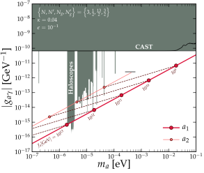
Figure 1: Photon coupling-mass relation for the two axion mass eigenstates $a_{1,2}$. We draw a dashed line to emphasize the connection between the two axions which is set by the value of the free parameter $\epsilon=f_{a}/f^{\prime}_{a}$. The lighter axion’s line cuts off at around $m_{2}\sim$ 0.4 meV when its heavier companion is excluded by stellar cooling. In gray we display some existing constraints from haloscope searches for DM Asztalos2010 ; ADMX:2018gho ; ADMX:2019uok ; ADMX:2018ogs ; Crisosto:2019fcj ; Lee:2020cfj ; Jeong:2020cwz ; CAPP:2020utb ; Devlin:2021fpq ; HAYSTAC:2018rwy ; HAYSTAC:2020kwv ; McAllister:2017lkb ; Alesini:2019ajt ; Alesini:2020vny ; CAST:2021add ; DePanfilis ; Hagmann , and helioscope searches for solar axions CAST:2007jps ; CAST:2017uph . We stress that these bounds are intended for illustration and context only, and we have not yet recast them into the companion-axion parameter space (see later figures).

When additional sources of PQ symmetry breaking are present, the effective axion potential gains another term,

$$V(a)=-2K\cos\left(N\frac{a}{f_{a}}+\theta\right)-2\kappa K\cos\left(N_{g}\frac{a}{f_{a}}+\theta_{g}\right)~{},$$ (1)

where $N$ and $N_{g}$ denote model-dependent anomaly coefficients, and $f_{a}$ is the scale of PQ symmetry breaking. Here $K=\frac{m_{u}m_{d}}{(m_{u}+m_{d})}m^{2}_{\pi}f^{2}_{\pi}$ measures the contribution coming from QCD instantons, whereas the parameter $\kappa$ quantifies the relative strength of the additional contribution, estimated to be $\kappa\sim 0.04-0.6$ for gravitational instantons Chen:2021jcb .

Since the additional CP-violating $\theta_{g}$ parameter is unrelated to $\theta$ and a priori should be $\sim\mathcal{O}(1)$, the vacuum configuration of the single axion field is no longer able to cancel the undesired CP violating effects. Hence, axion models Weinberg:1977ma ; Wilczek:1977pj ; Kim:1979if ; Shifman:1979if ; Zhitnitsky:1980tq ; Dine:1981rt are not valid solutions to the strong CP problem unless the additional contribution is sufficiently small, $\kappa<10^{-9}$ Chen:2021jcb .

Perhaps the simplest way to solve this new CP problem is to propose another PQ symmetry, implying the existence of a ‘companion’ axion in the particle spectrum. Depending on their relative PQ scales, the solution presents the tantalizing possibility that two QCD axions could be seen in future experiments. In this paper, we begin an investigation into the phenomenology of this model by examining the detectability of the two axions via their couplings to the photon.

Before proceeding, we point out that multi-axion models are not a radically new idea. In particular, the string axiverse scenario Masso:1995tw ; Masso:2002ip ; Ringwald:2012hr ; Ringwald:2012cu ; Arvanitaki:2009fg ; Svrcek:2006yi ; Acharya:2010zx ; Cicoli:2012sz ; Jaeckel:2010ni ; Stott:2017hvl has inspired many recent studies of systems of coupled axions Kitajima:2014xla ; Marsh:2019bjr ; Cyncynates:2021yjw ; Reig:2021ipa ; Chadha-Day:2021uyt . Additional axions have also been introduced in the context of inflation Kim:2004rp ; Dimopoulos:2005ac , to enhance Agrawal:2017cmd or suppress Babu:1994id ; Dror:2020zru ; Dror:2021nyr couplings to the Standard Model, to explain astrophysical anomalies Higaki:2014qua , or as relics of some other high-energy physics Hu:2020cga . The ‘companion axion’ model that we investigate here is distinct in that it requires two coupled particles to solve the strong-CP problem. This will significantly restrain the parameter space compared to axiverse models.

The companion axion model.—Proposed in Chen:2021jcb , the companion-axion model protects the PQ solution to the strong CP problem from colored Eguchi-Hanson (CEH) instantons Boutaleb-Joutei:1979vmg by extending the original $U(1)_{\rm PQ}$ symmetry to $U(1)_{\rm PQ}\times U(1)^{\prime}_{\rm PQ}$. Once spontaneously broken, two pseudo-Goldstone axions appear, with the potential

$$V(a,a^{\prime})= -2K\cos\left(N\frac{a}{f_{a}}+N^{\prime}\frac{a^{\prime}}{f_{a}^{\prime}}+\theta\right)$$

$$-2\kappa K\cos\left(N_{g}\frac{a}{f_{a}}+N^{\prime}_{g}\frac{a^{\prime}}{f_{a}^{\prime}}+\theta_{g}\right)~{}.$$ (2)

The lowest energy state is then realized for the axion field expectation values that cancel out both CP-violating terms. As long as $NN^{\prime}_{g}\neq N^{\prime}N_{g}$, the strong CP problem can be dynamically resolved à la Peccei-Quinn.

The two axion states $a$ and $a^{\prime}$ are mixed through the interactions in Eq.(2). The mixing angle $\alpha$ between mass eigenstates $a_{1}$ and $a_{2}$ is,

$$\tan 2\alpha=\frac{2\epsilon(NN^{\prime}+\kappa N_{g}N^{\prime}_{g})}{(N^{2}+\kappa N^{2}_{g})-\epsilon^{2}(N^{\prime 2}+\kappa N^{\prime 2}_{g})}\,$$ (3)

where for convenience we parameterize the ratio of the two PQ scales, $\epsilon\equiv f_{a}/f^{\prime}_{a}$. The mass eigenstates are given by,

$$m_{1}^{2}=\frac{\Delta m^{2}}{2}+\frac{K}{f^{2}_{a}}\bigg{(}(N^{2}+\kappa N^{2}_{g})+\epsilon^{2}(N^{2}+\kappa N^{2}_{g})\bigg{)},$$ (4)

$$\Delta m^{2}=\frac{2K}{f^{2}_{a}}\bigg{[}4(NN^{\prime}+\kappa N_{g}N^{\prime}_{g})^{2}\epsilon^{2}$$

$$~{}~{}~{}~{}~{}~{}~{}~{}~{}~{}~{}~{}~{}~{}~{}~{}~{}~{}~{}~{}+\Big{(}(N^{2}+\kappa N^{2}_{g})-\epsilon^{2}(N^{\prime 2}+\kappa N^{\prime 2}_{g})\Big{)}^{2}\bigg{]}^{1/2}$$ (5)

where $\Delta m^{2}=m_{1}^{2}-m_{2}^{2}>0$, making $a_{1}$ always the heaviest axion. Without loss of generality we can assume $\epsilon\leq 1$.

The above expressions simplify significantly in two particular cases: a hierarchical regime, $f^{\prime}_{a}\gg f_{a}$, and a strong-mixing regime, $f^{\prime}_{a}\simeq f_{a}$.

1. Hierarchy: $\epsilon\ll 1$. Assuming all anomaly coefficients are of the same order, and ignoring terms $\sim\mathcal{O}(\kappa^{2})$, we obtain

$$m_{1}^{2}\approx\frac{2K\left(N^{2}+\kappa N_{g}^{2}\right)}{f_{a}^{2}}~{},$$ (6)

$$m_{2}^{2}\approx\frac{\kappa\left(NN_{g}^{\prime}-N_{g}N^{\prime}\right)^{2}}{N^{4}+\kappa N^{2}N_{g}^{2}}\epsilon^{2}m_{1}^{2}\sim\kappa\epsilon^{2}m_{1}^{2}\,.$$ (7)

The heavier axion [Eq.(6)] has a mass the same order as the standard QCD axion, while the mass of the second axion [Eq.(7)] is determined by the relative size of the additional CEH instanton contribution ($\sim\kappa$) and has a further $\epsilon$ suppression due to its higher PQ scale. The mixing between the two axions in this regime is small because,

$$\alpha\approx\frac{NN^{\prime}+\kappa N_{g}N_{g}^{\prime}}{N^{\prime 2}+\kappa N_{g}^{\prime 2}}\epsilon\sim\epsilon\ll 1\,.$$ (8)

2. Mixing: $\epsilon\simeq 1$. In this case we have instead,

$$m_{1}^{2}\approx\frac{2K}{f_{a}^{2}}\left[N^{2}+N^{\prime 2}+\kappa\frac{N^{2}N_{g}^{2}+N^{\prime 2}N_{g}^{\prime 2}}{N^{2}+N^{\prime 2}}\right]~{},$$ (9)

$$m_{2}^{2}\approx\frac{2K\kappa}{f_{a}^{2}}~{}\frac{N^{2}N_{g}^{\prime 2}+N^{\prime 2}N_{g}^{2}}{N^{2}+N^{\prime 2}}\sim\kappa m_{1}^{2}~{}$$ (10)

Once again, the mass of the heavier axion [Eq.(9)] is of the same order of magnitude as the mass of the standard QCD axion, while the mass of the lighter axion [Eq.(10)] is entirely defined by the CEH instantons. Unlike the hierarchical regime, the axions in this case are strongly mixed,

$$\tan 2\alpha\approx-\frac{2\left(NN^{\prime}+\kappa N_{g}N_{g}^{\prime}\right)}{\left(N^{2}-N^{\prime 2}\right)+\kappa\left(N_{g}^{2}-N_{g}^{\prime 2}\right)}~{}.$$ (11)

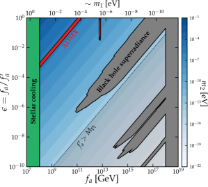
Figure 2: Left: Current bounds on the companion-axion model. The colorscale corresponds to the value of the lighter axion’s mass, whereas the heavier axion’s mass is shown (roughly) by the upper horizontal axis. We can rule out parts of this parameter space using stellar cooling arguments, ADMX, and black hole superradiance. Right: As in the left-hand panel, but now showing projected constraints from future experiments: MADMAX Beurthey:2020yuq , IAXO Armengaud:2019uso and DMRadio/ABRACADABRA DMRadio ; Kahn:2016aff .

Axion-photon couplings.—The couplings of the two axions to Standard Model fields can be computed using the usual techniques Srednicki:1985xd ; GrillidiCortona:2015jxo ; DiLuzio:2020wdo . To minimize the number of free parameters, we assume that the UV completion of the two-axion model is similar to the KSVZ model, popular in the single-QCD-axion case Kim:1979if ; Shifman:1979if . As such, the axions couple only to electrically neutral super-heavy quarks that carry charges under the extended $U(1)_{\rm PQ}\times U(1)^{\prime}_{\rm PQ}$ Peccei-Quinn symmetry. We then take suitable linear combinations of anomalous Peccei-Quinn and light-quark chiral currents and extract couplings of axion states $a$ and $a^{\prime}$ to the photon:

$$\mathcal{L}_{a\gamma}=\frac{1}{4}\left(ag_{a\gamma}+a^{\prime}g^{\prime}_{a\gamma}\right)F_{\mu\nu}\tilde{F}^{\mu\nu}~{},$$ (12)

where,

$$g_{a\gamma}=g^{\prime}_{a\gamma}\frac{f^{\prime}_{a}}{f_{a}}\frac{N}{N^{\prime}}=-\frac{\alpha_{\rm em}N}{2\pi f_{a}}\zeta,~{}~{}~{}\zeta=\frac{2}{3}\frac{4m_{d}+m_{u}}{m_{u}+m_{d}}~{},$$ (13)

where the factor $\zeta\approx 1.92$ is fixed to avoid the mixing of axions with QCD mesons Bardeen:1977bd . The photon couplings to the axion mass eigenstates can be readily obtained via,

$$g_{1} =\frac{\alpha_{\rm em}\zeta}{2\pi f_{a}}(N\cos\alpha-\epsilon N^{\prime}\sin\alpha)~{},$$ (14)

$$g_{2} =\frac{\alpha_{\rm em}\zeta}{2\pi f_{a}}(N\sin\alpha+\epsilon N^{\prime}\cos\alpha)\,.$$ (15)

The couplings $g_{1,2}$ as a function of $m_{1,2}$ are shown in Fig. 1. We choose representative values of the anomaly coefficients: $\{N,N^{\prime},N_{g},N^{\prime}_{g}\}=\{3,1/2,13/2,3/2\}$, and an instanton contribution ratio conservatively set to $\kappa=0.04$ Chen:2021jcb . The precise numbers are unimportant for our qualitative conclusions, but can lead to non-trivial quantitative differences to the couplings, including the possibility of cancellations.

In Fig. 1 we choose $\epsilon=f_{a}/f^{\prime}_{a}=10^{-1}$ such that the two axions are in the mixing regime and both of their masses can be displayed on the same plot. We can see that $a_{1}$ lies along the standard KSVZ line, whereas $a_{2}$ is always lighter. To provide familiar context, we have overlaid existing haloscope and helioscope constraints on the single-axion. The remainder of this work, however, will focus on re-deriving these constraints under the companion-axion model, including effects that are distinct from the single-axion case.

In our model we have two QCD axions and therefore two free parameters. Since we have fixed $f_{a}\leq f^{\prime}_{a}$, we can map existing and future constraints on our model by defining the parameter space $(f_{a},\epsilon)$, shown in Fig. 2. We use the color scale to encode the mass of the lighter state, $m_{2}$, where we see that constant values of $m_{2}$ roughly correspond to contours $\epsilon\propto f_{a}$. The mass of the heavier state $m_{1}$, in the hierarchical approximation [Eq.(6)], is shown by the upper horizontal axis. We now describe how we have derived each bound shown in this figure.

Stellar cooling.—Stars can be powerful factories for axions with masses smaller than their internal temperatures $\mathcal{O}($keV) Raffelt:2006cw . The most stringent bound on the photon coupling comes from the numbers of horizontal branch stars in globular clusters, whose lifetimes are sensitive to Primakoff production of axions $\gamma+Ze\rightarrow Ze+a$. Subsequently, single-axion-photon couplings,

$$\left|g_{a\gamma}\right|<6.6\times 10^{-11}\,{\rm GeV}^{-1}\,,$$ (16)

are ruled out at 95% C.L. Ayala:2014pea . This bound holds independently of the axion mass up to around $m_{a}\approx 30$ keV. We can convert this into a bound on the two-axion model by replacing $g_{a\gamma}$ in Eq. (16) with the electromagnetically active coupling combination $\tilde{g}=\sqrt{g_{1}^{2}+g_{2}^{2}}$ (see below). As would be expected, in the hierarchical case ($g_{2}\ll g_{1})$ the bound is the same as the single axion model because the lighter axion is not efficiently produced; whereas when $f_{a}\approx f^{\prime}_{a}$, both axions are generated by the star and the bound is enhanced by a factor $\sqrt{N^{2}+N^{\prime 2}}/N$.

Helioscopes.—A helioscope Sikivie:1983ip consists of a long magnetic bore pointed directly at the Sun, with a system of X-ray optics and detectors placed at the opposite end to capture solar axions converting into photons. For very light masses, the axion and photon oscillate coherently along the length of the magnet—in CAST, for example, their vacuum-mode limit holds for $m_{a}\lesssim 0.02$ eV. Above this mass, the momentum mismatch between the massive axions and the massless photon generates oscillations in the conversion probability over length-scales shorter than the experiment, suppressing the observable signal. The mass reach can be extended to the QCD axion band by providing the photon with a variable plasma mass which permits resonant conversion whenever the photon mass matches the axion mass—in CAST this is done by filling the bore with helium CAST:2013bqn ; CAST:2015qbl .

For helioscopes, unlike the stellar bounds, we must also consider the axion propagation to the detector. The two axions can be written in a basis where one particle state is an electromagnetically ‘active’ sum of the two axions, and the other state is ‘hidden’ Chadha-Day:2021uyt . The mixing angle of this system is given by,

$$\cos\theta=\frac{g_{1}}{\sqrt{g_{1}^{2}+g_{2}^{2}}}~{},$$ (17)

and the resulting off-diagonal term $M_{12}$ in the axion mass matrix is,

$$M_{12}=-\Delta m^{2}\frac{\cos^{2}\alpha}{1+\epsilon^{2}}\Big{(}\tan\alpha+\epsilon\big{(}1-\tan^{2}\alpha\big{)}-\epsilon^{2}\tan\alpha\Big{)}$$ (18)

While the Sun only emits the electromagnetically active state, the axions propagate in the mass-basis and so oscillate as they travel to Earth (see e.g. Chadha-Day:2021uyt ). Ultimately this will reduce the observable portion of the axion flux. The survival probability of the active axion with energy $\omega$, after travelling a distance $L$ is,

$$P =1-\sin^{2}2\theta\sin^{2}\left(\frac{\Delta m^{2}L}{4\omega}\right)~{},$$ (19)

where the first sine can be written in terms of our model parameters using Eqs.(14) and (17),

$$\sin^{2}2\theta =\frac{4\cos^{4}\alpha\left(\tan\alpha+\epsilon\left(1-\tan^{2}\alpha\right)-\epsilon^{2}\tan\alpha\right)^{2}}{\left(1+\epsilon^{2}\right)^{2}}$$

$$\approx\begin{cases}4\epsilon^{2},&\epsilon\ll 1\\ \cos^{2}2\alpha,&\epsilon\approx 1\end{cases}~{}.$$ (20)

Taking $L=1$ AU, and $\omega\sim$ keV, we can see that when $\Delta m^{2}\gtrsim 10^{-12}$ eV², or equivalently, $f_{a}\lesssim 10^{13}$ GeV, the axion-axion oscillation length is shorter than the Earth-Sun distance. As a result, the conversion probability will oscillate rapidly as a function of $\omega$, and the second sine in Eq.(19) averages to $1/2$. Since even next-generation helioscopes will only be sensitive to $f_{a}\lesssim 10^{9}$ GeV, we can assume we are always within this averaged regime.

Once the axions arrive at Earth they enter the strong transverse magnetic field of the helioscope, $B$, where the active axion state can now also oscillate into photons with $\tilde{g}B\omega$. While the three-particle oscillation problem is hard to solve analytically, we find that the axion-photon coupling is small compared to the coupling between the active and hidden axion. In the hierarchical case, $\tilde{g}=g\sqrt{1+\epsilon^{2})}\approx g$ and we can use Eq.(18) to find the ratio of these couplings,

$$\frac{\tilde{g}B\omega}{\Delta m^{2}\epsilon}=\frac{\alpha_{\rm em}\zeta B\omega}{4\pi K}f^{\prime}_{a}\lesssim 10^{-2},$$ (21)

where the upper limit is set by taking $f^{\prime}_{a}<M_{\rm pl}$. A similar relation holds in the strong-mixing regime. Since we are well within the regime where the two axions are mixed, we can therefore approximate the detected photon flux just as we would in the single-axion case, but reduced by the fraction of the population in the ‘active’ state. Any additional effects coming from the three-particle oscillation inside the experiment will be suppressed by the factor Eq.(21). Since the number of photons observed in a helioscope scales $\propto g_{a\gamma}^{4}$, we can recast existing and projected bounds by multiplying the minimum detectable photon coupling by the factor $P^{-1/4}$.

Just as with the single-axion, the CAST bounds are less sensitive than the stellar cooling bounds, so they do not appear on our plot. Instead, we show the projected bounds for the future helioscope IAXO Armengaud:2019uso . The result can be observed in Fig. 3, where we see that IAXO is expected to improve upon the stellar bound by just under an order of magnitude in $f_{a}$, and with a limit that is mostly insensitive to $\epsilon$—apart from in the strong-mixing regime where the axion-axion oscillations slightly impact the detectable flux. For this particular model configuration both axions could be seen during IAXO’s resonant buffer gas phase, however it may still be possible to measure the mass even in the vacuum phase if $a_{2}$ turned out to be lighter Dafni:2018tvj .

Haloscopes.—Axion haloscopes Sikivie:1983ip aim to detect axions constituting the DM halo of the Milky Way. In principle, rescaling past bounds set by experiments such as ADMX should be simple once we know the ratio of the local DM that is comprised of each axion. In the single axion case one can assume $\Omega_{a}=\Omega_{\rm dm}$ and remain agnostic towards how those axions were created. However, with two axions we are forced into making additional assumptions about their respective production mechanisms.

There are already complications involved in making a clear prediction for the cosmological abundance of axions when there is only one scale to deal with: including whether that scale is higher or lower than the scale of inflation, as well as the effects of topological defects Kawasaki:2014sqa ; Fleury:2015aca ; Klaer:2017ond ; Buschmann:2019icd ; Vaquero:2018tib ; Gorghetto:2018myk ; Gorghetto:2020qws ; Buschmann:2021sdq . In the companion axion scenario—where we have two scales—the situation is naturally more complicated. A more complete study of companion axion DM production in the early universe is therefore deserving of a full study newpaper (see also the recent Cyncynates:2021yjw ). However, to make progress we can adopt a crude estimate for the proportions of the DM made up of each axion. Assuming production by the misalignment mechanism alone (neglecting axions generated by topological defects), an order of magnitude estimate of the density ratio is,

$$\frac{\Omega_{a_{2}}}{\Omega_{a_{1}}}\sim\frac{\theta^{2}_{2}}{\theta_{1}^{2}}\kappa^{0.41}\epsilon^{-1.19},$$ (22)

valid for temperature-dependent axion masses, $m^{2}(T)\sim T^{-n}$, with $n=6.68$ Wantz:2009it . Unless $\epsilon\approx 1$ we expect the relic abundance to be dominated by the lighter axion. For our estimates we assume $\theta_{1}=\theta_{2}$, but if one or both of the PQ symmetries are broken before inflation these angles could be tuned to other values by anthropic arguments. Therefore, since our haloscope bounds are contingent on one particular cosmological scenario, they should be regarded as more model-dependent than single-axion bounds.

The companion-axion model offers an intriguing prospect for resonance-based haloscopes which must scan slowly across a mass range to search for a signal. Depending on $\Omega_{a_{1,2}}$, there could be a sizeable signal to be discovered at two distinct frequencies. But even if only one axion falls within reach of some experiment, a combined constraint on the companion-axion model can still be made. Since the model poses that both axions must exist, a constraint on a particular value of $f_{a}$ immediately implies that some $f^{\prime}_{a}=f_{a}/\epsilon$ is excluded as well. As such, we expect that a small section of some single-axion model that is ruled out by a haloscope to translate into two bands of ruled-out models in the $(f_{a},\epsilon)$ space, as in Fig. 2. ADMX currently excludes KSVZ axions around $m_{a}\sim 3\times 10^{-6}$ eV. When $\epsilon\gtrsim 10^{-2}$, ADMX excludes this same window because it would have seen the heavier axion there. However ADMX also excludes a diagonal band of smaller $f_{a}$ in the hierarchical regime, where the lighter axion would have been observed instead.

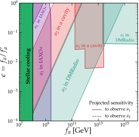
Figure 3: Projected sensitivity for loosely-defined future experiments: an upgraded version of IAXO Armengaud:2018cuy , resonant cavity experiments covering the 1–100 $\upmu$eV region (based on projections from Stern:2016bbw ), and DMRadio-like experiments covering the neV–$\upmu$eV region (based on DMRadio ). In the parts where the $a_{1}$ and $a_{2}$ regions overlap, the signal from both axions will be seen—a characteristic of the companion axion model. For some small regions the signal of the two axions could even be seen in the same experiment.

Black hole superradiance.—If light bosonic fields exist then they can form an exponentially growing bound state around a spinning BH. For fields with Compton wavelengths around the size of the BH ergoregion, the mechanism known as superradiance can act to extract the entirety of the BH’s spin Dolan:2007mj ; Arvanitaki:2010sy ; Pani:2012vp ; Brito:2015oca ; Arvanitaki:2014wva ; Arvanitaki:2016qwi ; Herdeiro:2016tmi ; Cardoso:2018tly ; Stott:2018opm . This means that the measurement of a BH spin can serve to rule out both axions if they have masses within the appropriate range.

The literature on this subject is developing, and there is not resounding agreement between the bounds derived by various groups Baryakhtar:2020gao ; Baryakhtar:2017ngi ; Stott:2020gjj ; Mehta:2020kwu ; Mehta:2021pwf who differ in both their theoretical and statistical treatments. We adopt the constraints derived using techniques described in Refs. Stott:2020gjj ; Mehta:2020kwu ; Mehta:2021pwf which cover both stellar and supermassive BHs. We assume that superradiance rules out both axion mass eigenstates but only when $f_{a}$ or $f^{\prime}_{a}$ are not below the scale where the bounds relax due to self-interactions. The four bands in Fig. 2 correspond to various stellar-mass and supermassive BHs with measured spins. We note however that different, more conservative bounds have also been derived Baryakhtar:2020gao using a more involved treatment of the field’s self-interactions, and neglecting supermassive BH spins which have been measured only at low significance. We should note also that the formation of the two axions’ bound states may proceed differently if there is mixing between the two eigenstates with different masses. Hence the bounds for $\epsilon$ close to 1 may not be accurate—although a detailed calculation of superradiance in this model is not our focus.

Discovering the companion axion model.—While for much of our parameter space one of the axions is rather light and weakly coupled, over the next few decades, plans are in place for experiments to scan almost the entirety of the QCD axion model band Irastorza:2018dyq . Therefore, we finish by estimating how much of our companion-axion parameter space would leave a unique signal in experiments.

In Fig. 3 we show the sensitivities of IAXO+ Armengaud:2019uso ; Armengaud:2014gea ; IAXO:2020wwp , as well as resonant-cavity McAllister:2017lkb ; Stern:2016bbw ; Melcon:2018dba ; AlvarezMelcon:2020vee ; Alesini:2017ifp ; Jeong:2017hqs and LC-circuit-based haloscopes Kahn:2016aff ; DMRadio ; Devlin:2021fpq ; Ouellet:2018beu ; Crisosto:2019fcj ; Gramolin:2020ict ; Salemi:2021gck . We opt here for the most ambitious projections that have been made—ones which essentially cover all of the QCD band above $m_{a}\sim$ neV. This space could also be covered by non-cavity haloscopes TheMADMAXWorkingGroup:2016hpc ; Schutte-Engel:2021bqm ; BRASS ; Lawson:2019brd ; Baryakhtar:2018doz , which we neglect to reduce clutter.

Helioscopes cannot probe above $f_{a}\sim 10^{9}$ GeV, meaning that some assumption about DM will be needed to explore further. For small $\epsilon$ and large $f_{a}$ there is a challenging region where no proposed experiments are sensitive. This is because the axion that dominates the DM abundance here is too weakly-coupled to detect in any proposed haloscope, and the low DM density in the heavier axion makes its signal too small to detect. It seems unlikely that experiments exploiting alternative couplings would be able to reach this regime either, but it may be possible to explore it via gravitational signatures Hook:2017psm ; Zhang:2021mks .

Conclusions.—Colored gravitational instantons jeopardize the single-axion solution to the strong-CP problem. A potential remedy, suggested by Ref. Chen:2021jcb , is to include a second “companion” axion that acts to remove the additional unwanted CP-violation. One axion is similar to the usual QCD axion that is being actively sought in experiments, whereas its companion would be present at some lighter mass. Both axions exist around the conventional QCD band, so the model would not demand any alterations to ongoing axion search campaigns. In fact, we predict that the signal of two axions may well appear, either in two different experiments, or perhaps even in the same experiment. One of the most remarkable messages that can be taken from this result is that even if an experiment does identify the signal of an axion, the remaining experiments operating at different frequencies should continue to search.

We have only delved into the implications for the photon coupling, which is just one dimension of the axion’s rich phenomenology. We anticipate many more interesting signals unique to the companion-axion model: for example via couplings to fermions Mitridate:2020kly ; Chigusa:2020gfs ; Ikeda:2021mlv ; QUAX:2020adt ; Crescini:2018qrz ; Aybas:2021nvn ; Garcon:2019inh ; JacksonKimball:2017elr ; Abel:2017rtm ; OHare:2020wah ; Arvanitaki:2014dfa ; JacksonKimball:2017elr , astrophysical signatures Hook:2017psm ; Hook:2018iia ; Dessert:2021bkv , or cosmological behavior newpaper . All of these may assist in either ruling out the remaining parameter space, or lead to an eventual discovery.

The figures from this article can be reproduced using the code available at https://github.com/cajohare/CompAxion, whereas the data for all the limits shown here is compiled at Ref AxionLimits .

Acknowledgements.—CAJO thanks Viraf Mehta and David Marsh for making available their superradiance constraints. The work of AK was partially supported by the Australian Research Council through the Discovery Project grant DP210101636 and by the Shota Rustaveli National Science Foundation of Georgia (SRNSFG) through the grant DI-18-335.

References

- (1) R. D. Peccei and H. R. Quinn, CP conservation in the presence of instantons, Phys. Rev. Lett. 38 (1977) 1440. [,328(1977)].
- (2) R. D. Peccei and H. R. Quinn, Constraints Imposed by CP Conservation in the Presence of Instantons, Phys. Rev. D 16 (1977) 1791.
- (3) nEDM Collaboration, C. Abel et al., Measurement of the permanent electric dipole moment of the neutron, Phys. Rev. Lett. 124 (2020) 081803 [2001.11966].
- (4) J. Preskill, M. B. Wise and F. Wilczek, Cosmology of the Invisible Axion, Phys. Lett. B 120 (1983) 127.
- (5) L. F. Abbott and P. Sikivie, A Cosmological Bound on the Invisible Axion, Phys. Lett. B 120 (1983) 133.
- (6) M. Dine and W. Fischler, The Not So Harmless Axion, Phys. Lett. B 120 (1983) 137.
- (7) D. J. E. Marsh, Axion cosmology, Phys. Rept. 643 (2016) 1 [1510.07633].
- (8) Z. Chen and A. Kobakhidze, Coloured gravitational instantons, the strong CP problem and the companion axion solution, 2108.05549.
- (9) S. J. Asztalos, G. Carosi, C. Hagmann, D. Kinion, K. van Bibber, M. Hotz, L. J. Rosenberg, G. Rybka, J. Hoskins, J. Hwang, P. Sikivie, D. B. Tanner, R. Bradley, J. Clarke and ADMX Collaboration, SQUID-Based Microwave Cavity Search for Dark-Matter Axions, Phys. Rev. Lett. 104 (2010) 041301 [0910.5914].
- (10) ADMX Collaboration, N. Du et al., A Search for Invisible Axion Dark Matter with the Axion Dark Matter Experiment, Phys. Rev. Lett. 120 (2018) 151301 [1804.05750].
- (11) ADMX Collaboration, T. Braine et al., Extended Search for the Invisible Axion with the Axion Dark Matter Experiment, Phys. Rev. Lett. 124 (2020) 101303 [1910.08638].
- (12) ADMX Collaboration, C. Boutan et al., Piezoelectrically Tuned Multimode Cavity Search for Axion Dark Matter, Phys. Rev. Lett. 121 (2018) 261302 [1901.00920].
- (13) N. Crisosto, P. Sikivie, N. S. Sullivan, D. B. Tanner, J. Yang and G. Rybka, ADMX SLIC: Results from a Superconducting Circuit Investigating Cold Axions, Phys. Rev. Lett. 124 (2020) 241101 [1911.05772].
- (14) S. Lee, S. Ahn, J. Choi, B. Ko and Y. Semertzidis, Axion Dark Matter Search around 6.7 eV, Phys. Rev. Lett. 124 (2020) 101802 [2001.05102].
- (15) J. Jeong, S. Youn, S. Bae, J. Kim, T. Seong, J. E. Kim and Y. K. Semertzidis, Search for Invisible Axion Dark Matter with a Multiple-Cell Haloscope, Phys. Rev. Lett. 125 (2020) 221302 [2008.10141].
- (16) CAPP Collaboration, O. Kwon et al., First Results from an Axion Haloscope at CAPP around 10.7 eV, Phys. Rev. Lett. 126 (2021) 191802 [2012.10764].
- (17) J. A. Devlin et al., Constraints on the Coupling between Axionlike Dark Matter and Photons Using an Antiproton Superconducting Tuned Detection Circuit in a Cryogenic Penning Trap, Phys. Rev. Lett. 126 (2021) 041301 [2101.11290].
- (18) HAYSTAC Collaboration, L. Zhong et al., Results from phase 1 of the HAYSTAC microwave cavity axion experiment, Phys. Rev. D 97 (2018) 092001 [1803.03690].
- (19) HAYSTAC Collaboration, K. M. Backes et al., A quantum-enhanced search for dark matter axions, Nature 590 (2021) 238 [2008.01853].
- (20) B. T. McAllister, G. Flower, E. N. Ivanov, M. Goryachev, J. Bourhill and M. E. Tobar, The ORGAN Experiment: An axion haloscope above 15 GHz, Phys. Dark Univ. 18 (2017) 67 [1706.00209].
- (21) D. Alesini et al., Galactic axions search with a superconducting resonant cavity, Phys. Rev. D 99 (2019) 101101 [1903.06547].
- (22) D. Alesini et al., Search for invisible axion dark matter of mass meV with the QUAX– experiment, Phys. Rev. D 103 (2021) 102004 [2012.09498].
- (23) CAST Collaboration, A. A. Melcón et al., First results of the CAST-RADES haloscope search for axions at 34.67 eV, 2104.13798.
- (24) S. DePanfilis, A. C. Melissinos, B. E. Moskowitz, J. T. Rogers, Y. K. Semertzidis, W. U. Wuensch, H. J. Halama, A. G. Prodell, W. B. Fowler and F. A. Nezrick, Limits on the abundance and coupling of cosmic axions at 4.55.0 ev, Phys. Rev. Lett. 59 (1987) 839.
- (25) C. Hagmann, P. Sikivie, N. S. Sullivan and D. B. Tanner, Results from a search for cosmic axions, Phys. Rev. D 42 (1990) 1297.
- (26) CAST Collaboration, S. Andriamonje et al., An Improved limit on the axion-photon coupling from the CAST experiment, JCAP 04 (2007) 010 [hep-ex/0702006].
- (27) CAST Collaboration, V. Anastassopoulos et al., New CAST Limit on the Axion-Photon Interaction, Nature Phys. 13 (2017) 584 [1705.02290].
- (28) S. Weinberg, A New Light Boson?, Phys. Rev. Lett. 40 (1978) 223.
- (29) F. Wilczek, Problem of Strong p and t Invariance in the Presence of Instantons, Phys. Rev. Lett. 40 (1978) 279.
- (30) J. E. Kim, Weak interaction singlet and Strong CP invariance, Phys. Rev. Lett. 43 (1979) 103.
- (31) M. A. Shifman, A. I. Vainshtein and V. I. Zakharov, Can Confinement Ensure Natural CP Invariance of Strong Interactions?, Nucl. Phys. B 166 (1980) 493.
- (32) A. R. Zhitnitsky, On Possible Suppression of the Axion Hadron Interactions. (In Russian), Sov. J. Nucl. Phys. 31 (1980) 260. [Yad. Fiz.31,497(1980)].
- (33) M. Dine, W. Fischler and M. Srednicki, A simple solution to the Strong CP Problem with a harmless axion, Phys. Lett. B 104 (1981) 199.
- (34) E. Masso and R. Toldra, On a light spinless particle coupled to photons, Phys. Rev. D 52 (1995) 1755 [hep-ph/9503293].
- (35) E. Masso, Axions and axion like particles, Nucl. Phys. B Proc. Suppl. 114 (2003) 67 [hep-ph/0209132].
- (36) A. Ringwald, Exploring the Role of Axions and Other WISPs in the Dark Universe, Phys. Dark Univ. 1 (2012) 116 [1210.5081].
- (37) A. Ringwald, Searching for axions and ALPs from string theory, J. Phys. Conf. Ser. 485 (2014) 012013 [1209.2299].
- (38) A. Arvanitaki, S. Dimopoulos, S. Dubovsky, N. Kaloper and J. March-Russell, String axiverse, Phys. Rev. D 81 (2010) 123530 [0905.4720].
- (39) P. Svrcek and E. Witten, Axions in string theory, JHEP 06 (2006) 051 [hep-th/0605206].
- (40) B. S. Acharya, K. Bobkov and P. Kumar, An M Theory Solution to the Strong CP Problem and Constraints on the Axiverse, JHEP 11 (2010) 105 [1004.5138].
- (41) M. Cicoli, M. Goodsell and A. Ringwald, The type IIB string axiverse and its low-energy phenomenology, JHEP 10 (2012) 146 [1206.0819].
- (42) J. Jaeckel and A. Ringwald, The low-energy frontier of particle physics, Ann. Rev. Nucl. Part. Sci. 60 (2010) 405 [1002.0329].
- (43) M. J. Stott, D. J. E. Marsh, C. Pongkitivanichkul, L. C. Price and B. S. Acharya, Spectrum of the axion dark sector, Phys. Rev. D 96 (2017) 083510 [1706.03236].
- (44) N. Kitajima and F. Takahashi, Resonant conversions of QCD axions into hidden axions and suppressed isocurvature perturbations, JCAP 01 (2015) 032 [1411.2011].
- (45) D. J. E. Marsh and W. Yin, Opening the 1 Hz axion window, JHEP 01 (2021) 169 [1912.08188].
- (46) D. Cyncynates, T. Giurgica-Tiron, O. Simon and J. O. Thompson, Friendship in the Axiverse: Late-time direct and astrophysical signatures of early-time nonlinear axion dynamics, 2109.09755.
- (47) M. Reig, The Stochastic Axiverse, 2104.09923.
- (48) F. Chadha-Day, Axion-like particle oscillations, 2107.12813.
- (49) J. E. Kim, H. P. Nilles and M. Peloso, Completing natural inflation, JCAP 01 (2005) 005 [hep-ph/0409138].
- (50) S. Dimopoulos, S. Kachru, J. McGreevy and J. G. Wacker, N-flation, JCAP 08 (2008) 003 [hep-th/0507205].
- (51) P. Agrawal, J. Fan, M. Reece and L.-T. Wang, Experimental Targets for Photon Couplings of the QCD Axion, JHEP 02 (2018) 006 [1709.06085].
- (52) K. S. Babu, S. M. Barr and D. Seckel, Axion dissipation through the mixing of Goldstone bosons, Phys. Lett. B 336 (1994) 213 [hep-ph/9406308].
- (53) J. A. Dror and J. M. Leedom, Cosmological Tension of Ultralight Axion Dark Matter and its Solutions, Phys. Rev. D 102 (2020) 115030 [2008.02279].
- (54) J. A. Dror, H. Murayama and N. L. Rodd, Cosmic axion background, Phys. Rev. D 103 (2021) 115004 [2101.09287].
- (55) T. Higaki, N. Kitajima and F. Takahashi, Hidden axion dark matter decaying through mixing with QCD axion and the 3.5 keV X-ray line, JCAP 12 (2014) 004 [1408.3936].
- (56) D. Hu, H.-R. Jiang, H.-L. Li, M.-L. Xiao and J.-H. Yu, Tale of two- axion models, Phys. Rev. D 103 (2021) 095025 [2009.01452].
- (57) H. Boutaleb-Joutei, A. Chakrabarti and A. Comtet, Gauge Field Configurations in Curved Space-times. 3. Selfdual SU(2) Fields in Eguchi-hanson Space, Phys. Rev. D 21 (1980) 979.
- (58) S. Beurthey et al., MADMAX Status Report, 2003.10894.
- (59) IAXO Collaboration, E. Armengaud et al., Physics potential of the International Axion Observatory (IAXO), JCAP 06 (2019) 047 [1904.09155].
- (60) https://irwinlab.sites.stanford.edu/dark-matter-radio-dmradio.
- (61) Y. Kahn, B. R. Safdi and J. Thaler, Broadband and Resonant Approaches to Axion Dark Matter Detection, Phys. Rev. Lett. 117 (2016) 141801 [1602.01086].
- (62) M. Srednicki, Axion Couplings to Matter. 1. CP Conserving Parts, Nucl. Phys. B 260 (1985) 689.
- (63) G. Grilli di Cortona, E. Hardy, J. Pardo Vega and G. Villadoro, The QCD axion, precisely, JHEP 01 (2016) 034 [1511.02867].
- (64) L. Di Luzio, M. Giannotti, E. Nardi and L. Visinelli, The landscape of QCD axion models, Phys. Rept. 870 (2020) 1 [2003.01100].
- (65) W. A. Bardeen and S. H. H. Tye, Current Algebra Applied to Properties of the Light Higgs Boson, Phys. Lett. B 74 (1978) 229.
- (66) G. G. Raffelt, Astrophysical axion bounds, Lect. Notes Phys. 741 (2008) 51 [hep-ph/0611350].
- (67) A. Ayala, I. Domínguez, M. Giannotti, A. Mirizzi and O. Straniero, Revisiting the bound on axion-photon coupling from Globular Clusters, Phys. Rev. Lett. 113 (2014) 191302 [1406.6053].
- (68) P. Sikivie, Experimental tests of the ”invisible” axion, Phys. Rev. Lett. 51 (1983) 1415.
- (69) CAST Collaboration, M. Arik et al., Search for Solar Axions by the CERN Axion Solar Telescope with 3He Buffer Gas: Closing the Hot Dark Matter Gap, Phys. Rev. Lett. 112 (2014) 091302 [1307.1985].
- (70) CAST Collaboration, M. Arik et al., New solar axion search using the CERN Axion Solar Telescope with 4He filling, Phys. Rev. D 92 (2015) 021101 [1503.00610].
- (71) T. Dafni, C. A. J. O’Hare, B. Lakić, J. Galán, F. J. Iguaz, I. G. Irastorza, K. Jakovčić, G. Luzón, J. Redondo and E. Ruiz Chóliz, Weighing the solar axion, Phys. Rev. D 99 (2019) 035037 [1811.09290].
- (72) M. Kawasaki, K. Saikawa and T. Sekiguchi, Axion dark matter from topological defects, Phys. Rev. D 91 (2015) 065014 [1412.0789].
- (73) L. Fleury and G. D. Moore, Axion dark matter: strings and their cores, JCAP 01 (2016) 004 [1509.00026].
- (74) V. B. Klaer and G. D. Moore, The dark-matter axion mass, JCAP 1711 (2017) 049 [1708.07521].
- (75) M. Buschmann, J. W. Foster and B. R. Safdi, Early-Universe Simulations of the Cosmological Axion, Phys. Rev. Lett. 124 (2020) 161103 [1906.00967].
- (76) A. Vaquero, J. Redondo and J. Stadler, Early seeds of axion miniclusters, JCAP 04 (2019) 012 [1809.09241].
- (77) M. Gorghetto, E. Hardy and G. Villadoro, Axions from Strings: the Attractive Solution, JHEP 07 (2018) 151 [1806.04677].
- (78) M. Gorghetto, E. Hardy and G. Villadoro, More Axions from Strings, SciPost Phys. 10 (2021) 050 [2007.04990].
- (79) M. Buschmann, J. W. Foster, A. Hook, A. Peterson, D. E. Willcox, W. Zhang and B. R. Safdi, Dark Matter from Axion Strings with Adaptive Mesh Refinement, 2108.05368.
- (80) C. Boehm, Z. Chen, A. Kobakhidze, C. A. J. O’Hare, Z. S. C. Picker and G. Pierobon, Cosmology of the companion axion model, In preparation (2021) .
- (81) O. Wantz and E. P. S. Shellard, Axion Cosmology Revisited, Phys. Rev. D 82 (2010) 123508 [0910.1066].
- (82) EDELWEISS Collaboration, E. Armengaud et al., Searches for electron interactions induced by new physics in the EDELWEISS-III Germanium bolometers, Phys. Rev. D 98 (2018) 082004 [1808.02340].
- (83) I. Stern, ADMX Status, PoS ICHEP2016 (2016) 198 [1612.08296].
- (84) S. R. Dolan, Instability of the massive Klein-Gordon field on the Kerr spacetime, Phys. Rev. D 76 (2007) 084001 [0705.2880].
- (85) A. Arvanitaki and S. Dubovsky, Exploring the String Axiverse with Precision Black Hole Physics, Phys. Rev. D 83 (2011) 044026 [1004.3558].
- (86) P. Pani, V. Cardoso, L. Gualtieri, E. Berti and A. Ishibashi, Black hole bombs and photon mass bounds, Phys. Rev. Lett. 109 (2012) 131102 [1209.0465].
- (87) R. Brito, V. Cardoso and P. Pani, Superradiance: Energy Extraction, Black-Hole Bombs and Implications for Astrophysics and Particle Physics, vol. 906. Springer, 2015, 10.1007/978-3-319-19000-6, [1501.06570].
- (88) A. Arvanitaki, M. Baryakhtar and X. Huang, Discovering the QCD Axion with Black Holes and Gravitational Waves, Phys. Rev. D 91 (2015) 084011 [1411.2263].
- (89) A. Arvanitaki, M. Baryakhtar, S. Dimopoulos, S. Dubovsky and R. Lasenby, Black Hole Mergers and the QCD Axion at Advanced LIGO, Phys. Rev. D 95 (2017) 043001 [1604.03958].
- (90) C. Herdeiro, E. Radu and H. Rúnarsson, Kerr black holes with Proca hair, Class. Quant. Grav. 33 (2016) 154001 [1603.02687].
- (91) V. Cardoso, O. J. C. Dias, G. S. Hartnett, M. Middleton, P. Pani and J. E. Santos, Constraining the mass of dark photons and axion-like particles through black-hole superradiance, JCAP 03 (2018) 043 [1801.01420].
- (92) M. J. Stott and D. J. E. Marsh, Black hole spin constraints on the mass spectrum and number of axionlike fields, Phys. Rev. D 98 (2018) 083006 [1805.02016].
- (93) M. Baryakhtar, M. Galanis, R. Lasenby and O. Simon, Black hole superradiance of self-interacting scalar fields, Phys. Rev. D 103 (2021) 095019 [2011.11646].
- (94) M. Baryakhtar, R. Lasenby and M. Teo, Black Hole Superradiance Signatures of Ultralight Vectors, Phys. Rev. D 96 (2017) 035019 [1704.05081].
- (95) M. J. Stott, Ultralight Bosonic Field Mass Bounds from Astrophysical Black Hole Spin, 2009.07206.
- (96) V. M. Mehta, M. Demirtas, C. Long, D. J. E. Marsh, L. Mcallister and M. J. Stott, Superradiance Exclusions in the Landscape of Type IIB String Theory, 2011.08693.
- (97) V. M. Mehta, M. Demirtas, C. Long, D. J. E. Marsh, L. McAllister and M. J. Stott, Superradiance in string theory, JCAP 07 (2021) 033 [2103.06812].
- (98) I. G. Irastorza and J. Redondo, New experimental approaches in the search for axion-like particles, Prog. Part. Nucl. Phys. 102 (2018) 89 [1801.08127].
- (99) E. Armengaud et al., Conceptual design of the international axion observatory (IAXO), JINST 9 (2014) T05002 [1401.3233].
- (100) IAXO Collaboration, A. Abeln et al., Conceptual design of BabyIAXO, the intermediate stage towards the International Axion Observatory, JHEP 05 (2021) 137 [2010.12076].
- (101) A. A. Melcón et al., Axion Searches with Microwave Filters: the RADES project, JCAP 05 (2018) 040 [1803.01243].
- (102) A. Álvarez Melcón et al., Scalable haloscopes for axion dark matter detection in the 30eV range with RADES, JHEP 07 (2020) 084 [2002.07639].
- (103) D. Alesini, D. Babusci, D. Di Gioacchino, C. Gatti, G. Lamanna and C. Ligi, The KLASH Proposal, 1707.06010.
- (104) J. Jeong, S. Youn, S. Ahn, J. E. Kim and Y. K. Semertzidis, Concept of multiple-cell cavity for axion dark matter search, Phys. Lett. B 777 (2018) 412 [1710.06969].
- (105) J. L. Ouellet et al., First Results from ABRACADABRA-10 cm: A Search for Sub-eV Axion Dark Matter, Phys. Rev. Lett. 122 (2019) 121802 [1810.12257].
- (106) A. V. Gramolin, D. Aybas, D. Johnson, J. Adam and A. O. Sushkov, Search for axion-like dark matter with ferromagnets, Nature Phys. 17 (2021) 79 [2003.03348].
- (107) C. P. Salemi et al., Search for Low-Mass Axion Dark Matter with ABRACADABRA-10 cm, Phys. Rev. Lett. 127 (2021) 081801 [2102.06722].
- (108) MADMAX Working Group Collaboration, A. Caldwell, G. Dvali, B. Majorovits, A. Millar, G. Raffelt, J. Redondo, O. Reimann, F. Simon and F. Steffen, Dielectric Haloscopes: A New Way to Detect Axion Dark Matter, Phys. Rev. Lett. 118 (2017) 091801 [1611.05865].
- (109) J. Schütte-Engel, D. J. E. Marsh, A. J. Millar, A. Sekine, F. Chadha-Day, S. Hoof, M. N. Ali, K.-C. Fong, E. Hardy and L. Šmejkal, Axion quasiparticles for axion dark matter detection, JCAP 08 (2021) 066 [2102.05366].
- (110) https://www1.physik.uni-hamburg.de/iexp/gruppe-horns/forschung/brass.html.
- (111) M. Lawson, A. J. Millar, M. Pancaldi, E. Vitagliano and F. Wilczek, Tunable axion plasma haloscopes, Phys. Rev. Lett. 123 (2019) 141802 [1904.11872].
- (112) M. Baryakhtar, J. Huang and R. Lasenby, Axion and hidden photon dark matter detection with multilayer optical haloscopes, Phys. Rev. D98 (2018) 035006 [1803.11455].
- (113) A. Hook and J. Huang, Probing axions with neutron star inspirals and other stellar processes, JHEP 06 (2018) 036 [1708.08464].
- (114) J. Zhang, Z. Lyu, J. Huang, M. C. Johnson, L. Sagunski, M. Sakellariadou and H. Yang, First Constraints on Light Axions from the Binary Neutron Star Gravitational Wave Event GW170817, 2105.13963.
- (115) A. Mitridate, T. Trickle, Z. Zhang and K. M. Zurek, Detectability of Axion Dark Matter with Phonon Polaritons and Magnons, Phys. Rev. D 102 (2020) 095005 [2005.10256].
- (116) S. Chigusa, T. Moroi and K. Nakayama, Detecting light boson dark matter through conversion into a magnon, Phys. Rev. D 101 (2020) 096013 [2001.10666].
- (117) T. Ikeda, A. Ito, K. Miuchi, J. Soda, H. Kurashige and Y. Shikano, Axion search with quantum nondemolition detection of magnons, 2102.08764.
- (118) QUAX Collaboration, N. Crescini et al., Axion search with a quantum-limited ferromagnetic haloscope, Phys. Rev. Lett. 124 (2020) 171801 [2001.08940].
- (119) N. Crescini et al., Operation of a ferromagnetic axion haloscope at eV, Eur. Phys. J. C 78 (2018) 703 [1806.00310]. [Erratum: Eur.Phys.J.C 78, 813 (2018)].
- (120) D. Aybas et al., Search for Axionlike Dark Matter Using Solid-State Nuclear Magnetic Resonance, Phys. Rev. Lett. 126 (2021) 141802 [2101.01241].
- (121) A. Garcon et al., Constraints on bosonic dark matter from ultralow-field nuclear magnetic resonance, Sci. Adv. 5 (2019) eaax4539 [1902.04644].
- (122) D. Jackson Kimball et al., Overview of the Cosmic Axion Spin Precession Experiment (CASPEr), Springer Proc. Phys. 245 (2020) 105 [1711.08999].
- (123) C. Abel et al., Search for Axionlike Dark Matter through Nuclear Spin Precession in Electric and Magnetic Fields, Phys. Rev. X 7 (2017) 041034 [1708.06367].
- (124) C. A. J. O’Hare and E. Vitagliano, Cornering the axion with -violating interactions, Phys. Rev. D 102 (2020) 115026 [2010.03889].
- (125) A. Arvanitaki and A. A. Geraci, Resonantly Detecting Axion-Mediated Forces with Nuclear Magnetic Resonance, Phys. Rev. Lett. 113 (2014) 161801 [1403.1290].
- (126) A. Hook, Y. Kahn, B. R. Safdi and Z. Sun, Radio signals from axion dark matter conversion in neutron Star magnetospheres, Phys. Rev. Lett. 121 (2018) 241102 [1804.03145].
- (127) C. Dessert, A. J. Long and B. R. Safdi, No evidence for axions from Chandra observation of magnetic white dwarf, 2104.12772.
- (128) C. O’Hare, cajohare/axionlimits: Axionlimits, July, 2020. 10.5281/zenodo.3932430.