Compressive Visual Representations

Abstract

Learning effective visual representations that generalize well without human supervision is a fundamental problem in order to apply Machine Learning to a wide variety of tasks. Recently, two families of self-supervised methods, contrastive learning and latent bootstrapping, exemplified by SimCLR and BYOL respectively, have made significant progress. In this work, we hypothesize that adding explicit information compression to these algorithms yields better and more robust representations. We verify this by developing SimCLR and BYOL formulations compatible with the Conditional Entropy Bottleneck (CEB) objective, allowing us to both measure and control the amount of compression in the learned representation, and observe their impact on downstream tasks. Furthermore, we explore the relationship between Lipschitz continuity and compression, showing a tractable lower bound on the Lipschitz constant of the encoders we learn. As Lipschitz continuity is closely related to robustness, this provides a new explanation for why compressed models are more robust. Our experiments confirm that adding compression to SimCLR and BYOL significantly improves linear evaluation accuracies and model robustness across a wide range of domain shifts. In particular, the compressed version of BYOL achieves 76.0% Top-1 linear evaluation accuracy on ImageNet with ResNet-50, and 78.8% with ResNet-50 2x.

1 Introduction

Individuals develop mental representations of the surrounding world that generalize over different views of a shared context. For instance, a shared context could be the identity of an object, as it does not change when viewed from different perspectives or lighting conditions. This ability to represent views by distilling information about the shared context has motivated a rich body of self-supervised learning work oord2018representation ; bachman2019learning ; chen2020simple ; grill2020bootstrap ; he2020momentum ; lee2020predictive . For a concrete example, we could consider an image from the ImageNet training set russakovsky2015imagenet as a shared context, and generate different views by repeatedly applying different data augmentations. Finding stable representations of a shared context corresponds to learning a minimal high-level description since not all information is relevant or persistent. This explicit requirement of learning a concise representation leads us to prefer objectives that are compressive and only retain the relevant information.

Recent contrastive approaches to self-supervised visual representation learning aim to learn representations that maximally capture the mutual information between two transformed views of an image oord2018representation ; bachman2019learning ; chen2020simple ; he2020momentum ; hjelm2018learning . The primary idea of these approaches is that this mutual information corresponds to a general shared context that is invariant to various transformations of the input, and it is assumed that such invariant features will be effective for various downstream higher-level tasks. However, although existing contrastive approaches maximize mutual information between augmented views of the same input, they do not necessarily compress away the irrelevant information from these views chen2020simple ; he2020momentum . As shown in fischer2020conditional ; fischer2020ceb , retaining irrelevant information often leads to less stable representations and to failures in robustness and generalization, hampering the efficacy of the learned representations. An alternative state-of-the-art self-supervised learning approach is BYOL grill2020bootstrap , which uses a slow-moving average network to learn consistent, view-invariant representations of the inputs. However, it also does not explicitly capture relevant compression in its objective.

In this work, we modify SimCLR chen2020simple , a state-of-the-art contrastive representation method, by adding information compression using the Conditional Entropy Bottleneck (CEB) fischer2020ceb . Similarly, we show how BYOL grill2020bootstrap representations can also be compressed using CEB. By using CEB we are able to measure and control the amount of information compression in the learned representation fischer2020conditional , and observe its impact on downstream tasks. We empirically demonstrate that our compressive variants of SimCLR and BYOL, which we name C-SimCLR and C-BYOL, significantly improve accuracy and robustness to domain shifts across a number of scenarios. Our primary contributions are:

• Reformulations of SimCLR and BYOL such that they are compatible with information-theoretic compression using the Conditional Entropy Bottleneck fischer2020conditional .

• An exploration of the relationship between Lipschitz continuity, SimCLR, and CEB compression, as well as a simple, tractable lower bound on the Lipschitz constant. This provides an alternative explanation, in addition to the information-theoretic view fischer2020conditional ; fischer2020ceb ; achille2017emergence ; achille2018information , for why CEB compression improves SimCLR model robustness.

• Extensive experiments supporting our hypothesis that adding compression to the state-of-the-art self-supervised representation methods like SimCLR and BYOL can significantly improve their performance and robustness to domain shifts across multiple datasets. In particular, linear evaluation accuracies of C-BYOL are even competitive with the supervised baselines considered by SimCLR chen2020simple and BYOL grill2020bootstrap . C-BYOL reaches 76.0% and 78.8% with ResNet-50 and ResNet-50 2x respectively, whereas the corresponding supervised baselines are 76.5% and 77.8% respectively.

2 Methods

In this section, we describe the components that allow us to make distributional, compressible versions of SimCLR and BYOL. This involves switching to the Conditional Entropy Bottleneck (CEB) objective, noting that the von Mises-Fisher distribution is the exponential family distribution that corresponds to the cosine similarity loss function used by SimCLR and BYOL, and carefully identifying the random variables and the variational distributions needed for CEB in SimCLR and BYOL. We also note that SimCLR and CEB together encourage learning models with a smaller Lipschitz constant, although they do not explicitly enforce that the Lipschitz constant be small.

2.1 The Conditional Entropy Bottleneck

In order to test our hypothesis that compression can improve visual representation quality, we need to be able to measure and control the amount of compression in our visual representations. To achieve this, we use the Conditional Entropy Bottleneck (CEB) (fischer2020conditional, ), an objective function in the Information Bottleneck (IB) (tishby2000information, ) family.

Given an observation $X$, a target $Y$, and a learned representation $Z$ of $X$, CEB can be written as:

$$CEB \equiv\min_{Z}\beta I(X;Z|Y)-I(Y;Z)$$ (1)

$$=\min_{Z}\beta(H(Z)-H(Z|X)-H(Z)+H(Z|Y))-H(Y)+H(Y|Z)$$ (2)

$$=\min_{Z}\beta(-H(Z|X)+H(Z|Y))+H(Y|Z)$$ (3)

where $H(\cdot)$ and $H(\cdot|\cdot)$ denote entropy and conditional entropy respectively. We can drop the $H(Y)$ term because it is constant with respect to $Z$. $I(Y;Z)$ is the useful information relevant to the task, or the prediction target $Y$. $I(X;Z|Y)$ is the residual information $Z$ captures about $X$ when we already know $Y$, which we aim to minimize. Compression strength increases as $\beta$ increases.

We define $e(z|x)$ as the true encoder distribution, where $z$ is sampled from; $b(z|y)$, a variational approximation conditioned on $y$; $d(y|z)$, the decoder distribution (also a variational approximation) which predicts $y$ conditioned on $z$. As shown in fischer2020conditional , CEB can be variationally upper-bounded:

$$vCEB \equiv\min_{e(z|x),b(z|y),d(y|z)}\mathbb{E}_{x,y\sim p(x,y),z\sim e(z|x)}\beta(\log e(z|x)-\log b(z|y))-\log d(y|z)$$ (4)

There is no requirement that all three distributions have learned parameters. At one limit, a model’s parameters can be restricted to any one of the three distributions; at the other limit, all three distributions could have learned parameters. If $e(\cdot)$ has learned parameters, its distributional form may be restricted, as we must be able to take gradients through the $z$ samples. The only requirement on the $b(\cdot)$ and $d(\cdot)$ distributions is that we be able to take gradients through their log probability functions.

InfoNCE.

As shown in fischer2020conditional , besides parameterizing $d(y|z)$, it is possible to reuse $b(z|y)$ to make a variational bound on the $H(Y|Z)$ term. As $I(Y;Z)=H(Y)-H(Y|Z)$ and $H(Y)$ is a constant with respect to $Z$:

$$H(Y|Z)\leq E_{x,y\sim p(x,y),z\sim e(z|x)}\log\frac{b(z|y)}{\sum_{k=1}^{K}b(z|y_{k})}$$ (5)

where $K$ is the number of examples in a minibatch. Eq. (5) is also known as the contrastive InfoNCE bound oord2018representation ; vmibounds . The inner term,

$$d(y|z)\equiv\frac{b(z|y)}{\sum_{k=1}^{K}b(z|y_{k})},$$ (6)

is a valid variational approximation of the true but unknown $p(y|z)$. Fischer fischer2020conditional calls Eq. (6) the CatGen decoder because it is a categorical distribution over the minibatch that approximates the generative decoder distribution.

2.2 C-SimCLR: Compressed SimCLR

The InfoNCE bound oord2018representation enables many contrastive visual representation methods to use it to capture shared context between different views of an image as a self-supervised objective chen2020simple ; chen2020big ; he2020momentum ; chen2020exploring ; hjelm2018learning . In this work, we show how to compress the SimCLR chen2020simple model, but the method we discuss is generally applicable to other InfoNCE-based models.

SimCLR applies randomized augmentations to an image to create two different views, $x$ and $y$ (which we also refer to as $x^{\prime}$), and encodes both of them with a shared encoder, producing representations $r_{x}$ and $r_{y}$. Both $r_{x}$ and $r_{y}$ are $l_{2}$-normalized. The SimCLR version of the InfoNCE objective is:

$$L_{NCE}(r_{x},r_{y})=-\log\frac{e^{\frac{1}{\tau}r_{y}^{T}r_{x}}}{\sum_{k=1}^{K}e^{\frac{1}{\tau}r_{y_{k}}^{T}r_{x}}}$$ (7)

where $\tau$ is a temperature term and $K$ is the number of views in a minibatch. SimCLR further makes its InfoNCE objective bidirectional, such that the final objective becomes

$$L_{NCE}(r_{x},r_{y})+L_{NCE}(r_{y},r_{x})=-\log\frac{e^{\frac{1}{\tau}r_{y}^{T}r_{x}}}{\sum_{k=1}^{K}e^{\frac{1}{\tau}r_{y_{k}}^{T}r_{x}}}-\log\frac{e^{\frac{1}{\tau}r_{x}^{T}r_{y}}}{\sum_{k=1}^{K}e^{\frac{1}{\tau}r_{x_{k}}^{T}r_{y}}}$$ (8)

We can observe the following: $\exp(\frac{1}{\tau}r_{y}^{T}r_{x})$ in Eq. (7) corresponds to the unnormalized $b(z|y)$ in Eq. (5). $e(\cdot|x)$ generates $z=r_{x}$, whilst $r_{y}$ and $r_{y_{k}}$ are distribution parameters of $b(\cdot|y)$ and $b(\cdot|y_{k})$ respectively. $e(\cdot|x)$ and $b(\cdot|y)$ share model parameters.

von Mises-Fisher Distributional Representations.

The cosine-similarity-based loss (Eq. (7)) is commonly used in contrastive learning and can be connected to choosing the von Mises-Fisher (vMF) distribution for $e(\cdot|x)$ and $b(\cdot|y)$ hasnat2017mises ; wang2020understanding . vMF is a distribution on the $(n-1)$-dimensional hyper-sphere. The probability density function is given by $f_{n}(z,\mu,\kappa)=C_{n}(\kappa)e^{\kappa\mu^{T}z}$, where $\mu$ and $\kappa$ are denoted as the mean direction and concentration parameter respectively. We assume $\kappa$ is a constant. The normalization term $C_{n}(\kappa)$ is a function of $\kappa$ and equal to $\frac{\kappa^{n/2-1}}{(2\pi)^{n/2}I_{n/2-1}(\kappa)}$, where $I_{v}$ denotes the modified Bessel function of the first kind at order $v$.

By setting the mean direction $\mu$ to $r_{y}$, concentration $\kappa_{b}$ of $b(\cdot|y)$ to $1/\tau$, and $r_{x}$ to $z$, we can connect the SimCLR objective (Eq. (7)) to the distributional form of InfoNCE (Eq. (5))

$$\frac{e^{\frac{1}{\tau}r_{y}^{T}r_{x}}}{\sum_{k=1}^{K}e^{\frac{1}{\tau}r_{y_{k}}^{T}r_{x}}}=\frac{C_{n}(\kappa_{b})e^{\kappa_{b}r_{y}^{T}r_{x}}}{\sum_{k=1}^{K}C_{n}(\kappa_{b})e^{\kappa_{b}r_{y_{k}}^{T}r_{x}}}=\frac{f_{n}(r_{x},r_{y},\kappa_{b})}{\sum_{k=1}^{K}f_{n}(r_{x},r_{y_{k}},\kappa_{b})}=\frac{b(r_{x}|y)}{\sum_{k=1}^{K}b(r_{x}|y_{k})}$$ (9)

$z=r_{x}$ is a deterministic unit-length vector, so we can view $e(\cdot|x)$ as a spherical delta distribution, which is equivalent to a vMF with $r_{x}$ as the mean direction and $\kappa_{e}\rightarrow\infty$. We can further extend the forward encoder to have non-infinite $\kappa_{e}$, which results in a stochastic $z$. These allow us to have SimCLR in a distributional form with explicit distributions $e(\cdot|x)$ and $b(\cdot|y)$ and satisfy the requirements of CEB discussed in Sec. 2.1.

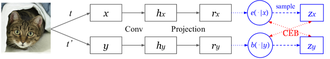
Figure 1: C-SimCLR explicitly defines encoder distributions $e(\cdot|x)$ and $b(\cdot|y)$ where $x$ and $y$ are two augmented views of an image. $y$ is also referred as $x^{\prime}$. The upper and lower encoder outputs are used to specify mean directions of $e$ and $b$, and the two encoders share parameters. $r_{x},r_{y}$ are $l_{2}$-normalized. Our modifications to SimCLR are highlighted in blue. No new parameters are added.

Compressing SimCLR with Bidirectional CEB.

Figure 1 illustrates the Compressed SimCLR (C-SimCLR) model. The model learns a compressed representation of an view $X$ that only preserves information relevant to predicting a different view $Y$ by switching to CEB. As can be seen in Eq. (3), the CEB objective treats $X$ and $Y$ asymmetrically. However, as shown in fischer2020conditional , it is possible to learn a single representation $Z$ of both $X$ and $Y$ by having the forward and backward encoders act as variational approximations of each other:

$$CEB_{\text{bidir}} \equiv\min_{Z}\beta_{X}I(X;Z|Y)-I(Y;Z)+\beta_{Y}I(Y;Z|X)-I(X;Z)$$ (10)

$$\equiv\min_{Z}\beta_{X}(-H(Z|X)+H(Z|Y))+H(Y|Z)$$ (11)

$$~{}~{}~{}~{}~{}~{}~{}~{}~{}~{}~{}~{}+\beta_{Y}(-H(Z|Y)+H(Z|X))+H(X|Z)$$

$$\leq\min_{e(\cdot|\cdot),b(\cdot|\cdot),c(\cdot|\cdot),d(\cdot|\cdot)}\mathbb{E}_{x,y\sim p(x,y)}\Big{[}$$ (12)

$$~{}~{}~{}~{}~{}~{}~{}~{}~{}~{}~{}~{}~{}~{}~{}~{}~{}~{}\mathbb{E}_{z_{x}\sim e(z_{x}|x)}\big{[}\beta_{X}(\log e(z_{x}|x)-\log b(z_{x}|y))-\log d(y|z_{x})\big{]}$$

$$~{}~{}~{}~{}~{}~{}~{}~{}~{}~{}~{}~{}~{}~{}~{}~{}~{}~{}+\mathbb{E}_{z_{y}\sim e(z_{y}|y)}\big{[}\beta_{Y}(\log(e(z_{y}|y)-\log(b(z_{y}|x))-\log c(x|z_{y})\big{]}\Big{]}$$

where $d(\cdot|\cdot)$ and $c(\cdot|\cdot)$ are the InfoNCE variational distributions of $b(\cdot|\cdot)$ and $e(\cdot|\cdot)$ respectively. $e$ and $b$ use the same encoder to parameterize mean direction in SimCLR setting. Since SimCLR is trained with a bidirectional InfoNCE objective, Eq. (12) gives an easy way to compress its learned representation. As in SimCLR, the deterministic $h_{x}$ (in Fig. 1) is still the representation used on downstream classification tasks.

2.3 C-BYOL: Compressed BYOL

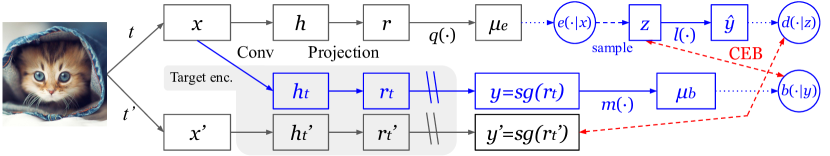
Figure 2: C-BYOL. The upper online encoder path takes an augmented view $x$ as input and produces $e(\cdot|x)$ and $d(\cdot|z)$. The lower two paths use the same target encoder (shaded), which is a moving average of the online encoder (Conv + Projection). The target encoder maps $x$ and another view $x^{\prime}$ to $r_{t}$ and $r_{t}^{\prime}$. $sg(r_{t})$ ($sg$: stop gradients) is our target $y$. $y$ leads to $b(\cdot|y)$. $sg(r_{t}^{\prime})$ is our perturbed target $y^{\prime}$. $r_{t},r_{t}^{\prime},\mu_{e},\mu_{b},\hat{y}$ are $l_{2}$-normalized. These yield the components required by CEB. We highlight changes to BYOL in blue.

In this section we will describe how to modify BYOL to make it compatible with CEB, as summarized in Fig. 2. BYOL grill2020bootstrap learns an online encoder that takes $x$, an augmented view of a given image, as input and predicts outputs of a target encoder which encodes $x^{\prime}$, a different augmented view of the same image. The target encoder’s parameters are updated not by gradients but as an exponential moving average of the online encoder’s parameters. The loss function is simply the mean square error, which is equivalent to the cosine similarity between the online encoder output $\mu_{e}$ and the target encoder output $y^{\prime}$ as both $\mu_{e}$ and $y^{\prime}$ are $l_{2}$-normalized:

$$L_{byol}=||\mu_{e}-y^{\prime}||^{2}_{2}=\mu_{e}^{T}\mu_{e}+{y^{\prime}}^{T}{y^{\prime}}-2\mu_{e}^{T}y^{\prime}=2-2\mu_{e}^{T}y^{\prime}$$ (13)

This iterative “latent bootstrapping” allows BYOL to learn a view-invariant representation. In contrast to SimCLR, BYOL does not rely on other samples in a batch and does not optimize the InfoNCE bound. It is a simple regression task: given input $x$, predict $y^{\prime}$. To make BYOL CEB-compatible, we need to identify the random variables $X$, $Y$, $Z$, define encoder distributions $e(z|x)$ and $b(z|y)$, and define the decoder distribution $d(y|z)$ (see Equation 4).

We define $e(z|x)$ to be a vMF distribution parameterized by $\mu_{e}$, and sample $z$ from $e(z|x)$:

$$e(z|x)=C_{n}(\kappa_{e})e^{\kappa_{e}z^{T}\mu_{e}}$$ (14)

We use the target encoder to encode $x$ and output $r_{t}$, an $l_{2}$-normalized vector. We choose $r_{t}$ to be $y$. We then add a 2-layer MLP on top of $y$ and $l_{2}$-normalize the output, which gives $\mu_{b}$. We denote this transformation as $\mu_{b}=m(y)$ and define $b(z|y)$ to be the following vMF parameterized by $\mu_{b}$:

$$b(z|y)=C_{n}(\kappa_{b})e^{\kappa_{b}z^{T}\mu_{b}}$$ (15)

For $d(y|z)$, we add a linear transformation on $z$ with $l_{2}$-normalization, $\hat{y}=l(z)$, and define a vMF parameterized by $\hat{y}$:

$$d(y|z)=C_{n}(\kappa_{d})e^{\kappa_{d}y^{T}\hat{y}}$$ (16)

In the deterministic case where $z$ is not sampled, this corresponds to adding a linear layer with $l_{2}$-normalization on $\mu_{e}$ which does not change the model capacity and empirical performance.

In principle, we can use any stochastic function of $Z$ to generate $Y$. In our implementation, we replace the generative decoder $\log d(y|z)$ with $\log d(y^{\prime}|z)$, where we use the target encoder to encode $x^{\prime}$ and output $y^{\prime}$. Given that $X\rightarrow X^{\prime}$ is a stochastic transformation and both $X$ and $X^{\prime}$ go through the same the target encoder function, $Y\rightarrow Y^{\prime}$ is also a stochastic transformation. $d(y^{\prime}|z)$ can be considered as having a stochastic perturbation to $d(y|z)$. Our $vCEB$ objective becomes

$$L_{cbyol}(x,x^{\prime})=\beta(\log e(z|x)-\log b(z|y))-\log d(y^{\prime}|z).$$ (17)

We empirically observed the best results with this design choice. $d(y^{\prime}|z)$ can be directly connected the standard BYOL regression objective: When $\kappa_{d}=2$, $-\log(d(y^{\prime}|z))=-\kappa_{d}y^{\prime T}\hat{y}-\log(C_{n}(\kappa_{d}))$ is equivalent to Eq. (13) when constants are ignored.

Although it seems that we additionally apply the target encoder to $x$ compared to BYOL, this does not increase the computational cost in practice. As in BYOL, the learning objective is applied symmetrically in our implementation: $L_{cbyol}(x,x^{\prime})+L_{cbyol}(x^{\prime},x)$. Therefore, the target encoder has to be applied to both $x$ and $x^{\prime}$ no matter in BYOL or C-BYOL. Finally, note that like in BYOL, $h$ (Fig. 2) is the deterministic representation used for downstream tasks.

2.4 Lipschitz Continuity and Compression

Lipschitz continuity provides a way of measuring how smooth a function is. For some function $f$ and a distance measure $D(f(x_{1}),f(x_{2}))$, Lipschitz continuity defines an upper bound on how quickly $f$ can change as $x$ changes:

$$L||\Delta x||\geq D(f(x),f(x+\Delta x)),$$ (18)

where $L$ is the Lipschitz constant, $\Delta x$ is the vector change in $x$, and $||\Delta x||>0$. If we define $f(x)$ to be our encoder distribution $e(z|x)$ (which is a vMF and always positive), and the distance measure, $D$, to be the absolute difference of the logs of the functions, we get a function of $z$ of Lipschitz value, such that:

$$L(z)\geq\frac{1}{||\Delta x||}|\log e(z|x)-\log e(z|x+\Delta x)|$$ (19)

As detailed in Sec. G, by taking expectations with respect to $z$, we can obtain a lower bound on the encoder distribution’s squared Lipschitz constant:

$$L^{2}\geq\frac{1}{||\Delta x||^{2}}\max\Big{(}\operatorname{KL}[e(z|x)||e(z|x+\Delta x)],\,\operatorname{KL}[e(z|x+\Delta x)||e(z|x)]\Big{)}$$ (20)

To guarantee smoothness of the encoder distribution, we would like to have an upper bound on $L$, rather than a lower bound. Minimizing a lower bound does not directly yield any optimality guarantees relative to the bounded quantity. However, in this case, minimizing the symmetric $\operatorname{KL}$ below is consistent with learning a smoother encoder function:

$$\inf_{e(z|\cdot)}\operatorname{KL}[e(z|x)||e(z|x+\Delta x)]+\operatorname{KL}[e(z|x+\Delta x)||e(z|x)]$$ (21)

By consistent, we mean that, if we could minimize this symmetric KL at every pair $(x,x+\Delta x)$ in the input domain, we would have smoothed the model. In practice, for high-dimensional input domains, that is not possible, but minimizing Eq. (21) at a subset of the input domain still improves the model’s smoothness, at least at that subset.

The minimization in Eq. (21) corresponds almost exactly to the CEB compression term in the bidirectional SimCLR models. We define $y=x+\Delta x$. At samples of the augmented observed variables, $X,Y$, the C-SimCLR models minimize upper bounds on the two residual informations:

$$I(X;Z|Y)+I(Y;Z|X)\leq\mathbb{E}_{x,y\sim p(x,y)}\operatorname{KL}[e(z|x)||e(z|y)]+\operatorname{KL}[e(z|y)||e(z|x)]$$ (22)

The only caveat to this is that we use $b(z|y)$ instead of $e(z|y)$ in C-SimCLR. $b$ and $e$ share weights but have different $\kappa$ values in their vMF distributions. However, these are hyperparameters, so they are not part of the trained model parameters. They simply change the minimum attainable $\operatorname{KL}$s in Eq. (22), thereby adjusting the minimum achievable Lipschitz constant for the models (see Sec. G).

Directly minimizing Equation 20 would require normalizing the symmetric $\operatorname{KL}$ per-example by $||\Delta x||^{2}$. The symmetric CEB loss does not do this. However, the residual information terms in Equation 22 are multiplied by a hyperparameter $\beta\leq 1$. Under a simplifying assumption that the $||\Delta x||$ values generated by the sampling procedure are typically of similar magnitude, we can extract the average $\frac{1}{||\Delta x||^{2}}$ into the hyperparameter $\beta$. We note that in practice using per-example values of $||\Delta x||^{2}$ would encourage the optimization process to smooth the model more strongly at observed $(x,\Delta x)$ pairs where it is least smooth, but we leave such experiments to future work.

Due to Eq. (22), we should expect that the C-SimCLR models are locally more smooth around the observed data points. We reiterate, though, that this is not a proof of increased global Lipschitz smoothness, as we are minimizing a lower bound on the Lipschitz constant, rather than minimizing an upper bound. It is still theoretically possible to learn highly non-smooth functions using CEB in this manner. It would be surprising, however, if the C-SimCLR were somehow less smooth than the corresponding SimCLR models.

The Lipschitz continuity property is closely related to model robustness to perturbations bruna2013invariant , including robustness to adversarial examples weng2018evaluating ; fazlyab2019efficient ; yang2020closer . Therefore, we would expect to see that the C-SimCLR models are more robust than SimCLR models on common robustness benchmarks. It is more difficult to make the same theoretical argument for the C-BYOL models, as they do not use exactly the same encoder for both $x$ and $y$. Thus, the equivalent conditional information terms from Eq. (22) are not directly minimizing a lower bound on the Lipschitz constant of the encoder. Nevertheless, we empirically explore the impact of CEB on both SimCLR and BYOL models next in Sec. 3.

3 Experimental Evaluation

We first describe our experimental set-up in Sec. 3.1, before evaluating the image representations learned by our self-supervised models in linear evaluation settings in Sec. 3.2. We then analyse the robustness and generalization of our self-supervised representations by evaluating model accuracy across a wide range of domain and distributional shifts in Sec. 3.3. Finally, we analyse the effect of compression strength in Sec. 3.4. Additional experiments and ablations can be found in the Appendix.

3.1 Experimental Set-up

Implementation details.

Our implementation of SimCLR, BYOL, and their compressed versions is based off of the public implementation of SimCLR chen2020simple . Our implementation consistently reproduces BYOL results from grill2020bootstrap and outperforms the original SimCLR, as detailed in Sec. A.

We use the same set of image augmentations as in BYOL grill2020bootstrap for both BYOL and SimCLR, and also use BYOL’s (4096, 256) two-layer projection head for both methods. We follow SimCLR and BYOL to use the LARS optimizer you2017large with a cosine decay learning rate schedule loshchilov2016sgdr over 1000 epochs with a warm-up period, as detailed in Sec. A.4. For ablation experiments we train for 300 epochs instead. As in SimCLR and BYOL, we use batch size of 4096 split over 64 Cloud TPU v3 cores. Except for ablation studies of compression strength, $\beta$ is set to $1.0$ for both C-SimCLR and C-BYOL. We follow SimCLR and BYOL in their hyperparameter choices unless otherwise stated, and provide exhaustive details in Sec. A. Pseudocode can be found in Sec. H.

Evaluation protocol.

We assess the performance of representations pretrained on the ImageNet training set russakovsky2015imagenet without using any labels. Then we train a linear classifier on different labeled datasets on top of the frozen representation. The final performance metric is the accuracy of these classifiers. As our approach builds on SimCLR chen2020big and BYOL grill2020bootstrap , we follow the same evaluation protocols. Further details are in Sec. B.

3.2 Linear Evaluation of Self-supervised Representations

Linear evaluation on ImageNet.

We first evaluate the representations learned by our models by training a linear classifier on top of frozen features on the ImageNet training set, following standard practice chen2020simple ; grill2020bootstrap ; kolesnikov2019revisiting ; kornblith2019better . As shown in Table 1, our compressed objectives provide strong improvements to state-of-the-art SimCLR chen2020simple and BYOL grill2020bootstrap models across different ResNet architectures he2016deep of varying widths (and thus number of parameters) zagoruyko2016wide . Our reproduction of the SimCLR baseline (70.7% top-1 accuracy) outperforms that of the original paper (69.3%). Our implementation of BYOL, which obtains a mean Top-1 accuracy of 74.2% (averaged over three trials) matches that of grill2020bootstrap within a standard deviation.

Current self-supervised methods benefit from longer training schedules chen2020simple ; chen2020big ; grill2020bootstrap ; chen2020exploring ; he2020momentum . Table 1 shows that our improvements remain consistent for both 300 epochs, and the longer 1000 epoch schedule which achieves the best results. In addition to the Top-1 and Top-5 accuracies, we also compute the Brier score brier1950verification which measures model calibration. Similar to the predictive accuracy, we observe that our compressed models obtain consistent improvements.

Table 1: ImageNet accuracy of linear classifiers trained on representations learned with SimCLR chen2020simple and BYOL grill2020bootstrap , with and without CEB compression. A lower Brier score corresponds to better model calibration. We report mean accuracy and standard deviations over three trials.

	SimCLR			BYOL
Method	Top-1	Top-5	Brier	Top-1	Top-5	Brier
ResNet-50, 300 epochs
Uncompressed	69.1$\pm 0.089$	89.1$\pm 0.034$	42.1$\pm 1.06$	72.8$\pm 0.155$	91.0$\pm 0.072$	37.3$\pm 0.089$
Compressed	70.1$\pm 0.177$	89.6$\pm 0.099$	41.0$\pm 0.107$	73.6$\pm 0.039$	91.5$\pm 0.080$	36.5$\pm 0.045$
ResNet-50, 1000 epochs
Uncompressed	70.7$\pm 0.094$	90.1$\pm 0.081$	40.0$\pm 0.123$	74.2$\pm 0.139$	91.7$\pm 0.041$	35.7$\pm{0.114}$
Compressed	71.6$\pm 0.084$	90.5$\pm 0.067$	39.7$\pm 0.876$	75.6$\pm 0.151$	92.7$\pm 0.076$	34.0$\pm 0.127$
ResNet-50 2x, 1000 epochs
Uncompressed	74.5$\pm 0.014$	92.1$\pm 0.031$	35.2$\pm{0.038}$	77.2$\pm 0.057$	93.5$\pm 0.036$	31.8$\pm{0.073}$
Compressed	75.0$\pm 0.082$	92.4$\pm 0.086$	34.7$\pm 0.129$	78.8$\pm 0.088$	94.5$\pm 0.016$	29.8$\pm 0.028$

Learning with a few labels on ImageNet.

Table 2: ImageNet accuracy when training linear classifiers with 1% and 10% of the labeled ImageNet data, on top of frozen, self-supervised representations learned on the entire ImageNet dataset without labels. For the supervised baseline, the whole ResNet-50 network is trained from random initialisation. We report mean results of 3 trials.

	Top-1		Top-5
Method	1%	10%	1%	10%
Supervised zhai2019s4l	25.4	56.4	48.4	80.4
SimCLR	49.3	63.3	75.8	85.9
C-SimCLR	51.1	64.5	77.2	86.5
BYOL	55.5	68.2	79.7	88.4
C-BYOL	60.6	70.5	83.4	90.0

Table 3: Comparison to other methods on ImageNet linear evaluation and supervised baselines. *: trained for 800 epochs. Other methods are 1000 epochs.

	ResNet-50
Method	1x	2x
SimCLR chen2020simple	69.3	74.2
SwAV* (2 crop) caron2020unsupervised ; chen2020exploring	71.8	-
InfoMin Aug* tian2020makes	73.0	-
Barlow Twins zbontar2021barlow	73.2	-
BYOL grill2020bootstrap	74.3	77.4
C-SimCLR (ours)	71.6	75.0
C-BYOL (ours)	75.6	78.8
Supervised chen2020simple ; grill2020bootstrap	76.5	77.8

After self-supervised pretraining on ImageNet, we learn a linear classifier on a small subset (1% or 10%) of the ImageNet training set, using the class labels this time, following the standard protocol of chen2020simple ; grill2020bootstrap . We expect that with strong feature representations, we should be able to learn an effective classifier with limited training examples.

Table 3 shows that the compressed models once again outperform the SimCLR and BYOL counterparts. The largest improvements are observed in the low-data regime, where we improve upon the state-of-the-art BYOL by 5.1% and SimCLR by 1.8%, when using only 1% of the ImageNet labels. Moreover, note that self-supervised representations significantly outperform a fully-supervised ResNet-50 baseline which overfits significantly in this low-data scenario.

Comparison to other methods.

Table 3 compares C-SimCLR and C-BYOL to other recent self-supervised methods from the literature (in the standard setting of using two augmented views) on ImageNet linear evaluation accuracy. We present accuracy for models trained for 800 and 1000 epochs, depending on what the original authors reported. C-BYOL achieves the best results compared to other state-of-the-art methods. Moreover, we can improve C-BYOL with ResNet-50 even further to 76.0 Top-1 accuracy when we train it for 1500 epochs.

Comparison to supervised baselines.

As shown in Table 3, SimCLR and BYOL use supervised baselines of 76.5% for ResNet-50 and 77.8% for ResNet-50 2x chen2020simple ; grill2020bootstrap respectively. In comparison, the corresponding compressed BYOL models achieve 76.0% for ResNet-50 and 78.8% for ResNet-50 2x, effectively matching or surpassing reasonable supervised baselines.

The results in Tables 1, 3 and 3 support our hypothesis that compression of SSL techniques can improve their ability to generalize in a variety of settings. These results are consistent with theoretical understandings of the relationship between compression and generalization shamir2008learning ; vera2018role ; dubois2020learning , as are the results in Table 5 that show that performance improves with increasingly strong compression (corresponding to higher values of $\beta$), up to some maximum amount of compression, after which performance degrades again.

3.3 Evaluation of Model Robustness and Generalization

In this section, we analyse the robustness of our models to various domain shifts. Concretely, we use the models, with their linear classifier, from the previous experiment, and evaluate them on a suite of robustness benchmarks that have the same label set as the ImageNet dataset. We use the public robustness benchmark evaluation code of djolonga2020robustness ; djolonga2020robustnesscode . As a result, we can evaluate our network and report Top-1 accuracy, as shown in Table 4, without any modifications to the network.

We consider “natural adversarial examples” with ImageNet-A hendrycks2019benchmarking which consists of difficult images which a ResNet-50 classifier failed on. ImageNet-C hendrycks2019benchmarking adds synthetic corruptions to the ImageNet validation set, ImageNet-R hendrycks2020many considers other naturally occuring distribution changes in image style while ObjectNet barbu2019objectnet presents a more difficult test set for ImageNet where the authors control for different parameters such as viewpoint and background. ImageNet-Vid and YouTube-BB shankar2019image evaluate the robustness of image classifiers to natural perturbations arising in video. Finally, ImageNet-v2 recht2019imagenet is a new validation set for ImageNet where the authors attempted to replicate the original data collection process. Further details of these robustness benchmarks are in Appendix F.

Table 4: Evaluation of robustness and generalization of self-supervised models, using a ResNet-50 backbone trained on ImageNet for 1000 epochs. We report the mean Top-1 accuracy over 3 trials on a range of benchmarks (detailed in Sec. 3.3 and the appendix) which measure an ImageNet-trained model’s generalization to different domains and distributions.

Method	ImageNet-A	ImageNet-C	ImageNet-R	ImageNet-v2	ImageNet-Vid	YouTube-BB	ObjectNet
SimCLR	1.3	35.0	18.3	57.7	63.8	57.3	18.7
C-SimCLR	1.4	36.8	19.6	58.7	64.7	59.5	20.8
BYOL	1.6	42.7	24.4	62.1	67.9	60.7	23.4
C-BYOL	2.3	45.1	25.8	63.9	70.8	63.6	25.5

Table 4 shows that SimCLR and BYOL models trained with CEB compression consistently outperform their uncompressed counterparts across all seven robustness benchmarks. This is what we hypothesized in the SimCLR settings based on the Lipschitz continuity argument in Sec. 2.4 and the appendix. All models performed poorly on ImageNet-A, but this is not surprising given that ImageNet-A was collected by hendrycks2019benchmarking according to images that a ResNet-50 classifier trained with full supervision on ImageNet misclassified, and we evaluate with ResNet-50 models too.

3.4 The Effect of Compression Strength

Table 5: Ablation study of CEB compression using C-SimCLR models trained for 300 epochs with a ResNet-50 backbone. $\beta$ controls the level of CEB compression. We evaluate linear-evaluation on ImageNet, and model robustness on the remaining datasets as described in Sec. 3.3.

Method	ImageNet	ImageNet-A	ImageNet-C	ImageNet-R	ImageNet-v2	ImageNet-Vid	YouTube-BB	ObjectNet
SimCLR	69.0	1.2	32.9	17.8	56.0	61.1	58.3	17.6
$\beta=0$	69.7	1.1	35.8	17.6	56.8	62.5	58.4	18.5
$\beta=0.01$	69.7	1.2	36.2	17.5	57.2	61.2	58.5	18.7
$\beta=0.1$	70.1	1.1	36.1	17.6	56.9	62.4	58.6	18.4
$\beta=1$	70.2	1.1	36.7	18.2	57.5	62.6	60.4	19.2
$\beta=1.5$	69.7	1.1	36.4	18.3	57.3	62.0	57.9	18.5

Table 5 studies the effect of the CEB compression term, $\beta$ on linear evaluation accuracy on ImageNet, as well as on the same suite of robustness datasets. We observe that $\beta=0$, which corresponds to no explicit compression, but a stochastic representation, already achieves improvements across all datasets. Further improvements are observed by increasing compression ($\beta$), with $\beta=1$ obtaining the best results. But overly strong compression can be harmful. Large values of $\beta$ correspond to high levels of compression, and can cause training to collapse, which we observed for $\beta=2$.

4 Related Work

Most methods for learning visual representations without additional annotation can be roughly grouped into three families: generative, discriminative, and bootstrapping. Generative approaches build a latent embedding that models the data distribution, but suffer from the expensive image generation step vincent2008extracting ; rezende2014stochastic ; goodfellow2014generative ; hinton2006fast ; kingma2013auto . While many early discriminative approaches used heuristic pretext tasks doersch2015unsupervised ; noroozi2016unsupervised , multi-view contrastive methods are among the recent state-of-the-art chen2020simple ; he2020momentum ; chen2020improved ; chen2020big ; oord2018representation ; henaff2020data ; li2021prototypical ; tian2019contrastive ; caron2020unsupervised .

Some previous contributions in the multi-view contrastive family tian2020makes ; zbontar2021barlow ; sridharan2008information ; dubois2021lossy can be connected to the information bottleneck principle tishby2000information ; tishby2015deep ; alemi2016deep but in a form of unconditional compression as they are agnostic of the prediction target, i.e. the target view in multiview contrastive learning. As discussed in fischer2020conditional ; fischer2020ceb , CEB performs conditional compression that directly optimizes for the information relevant to the task, and is shown theoretically and empirically better fischer2020conditional ; fischer2020ceb . A multi-view self-supervised formulation of CEB, which C-SimCLR can be linked to, was described in fischer2020conditional . Federici et al. federici2020learning later proposed a practical implementation of that, leveraging either label information or data augmentations. In comparison to federici2020learning , we apply our methods with large ResNet models to well-studied large-scale classification datasets like ImageNet and study improvements in robustness and generalization, rather than using two layer MLPs on smaller scale tasks. This shows that compression can still work using state-of-the-art models on challenging tasks. Furthermore, we use the vMF distribution rather than Gaussians in high-dimensional spaces, and extend beyond contrastive learning with C-BYOL.

Among the bootstrapping approaches guo2020bootstrap ; caron2018deep ; grill2020bootstrap which BYOL grill2020bootstrap belongs to, BYORL gowal2021selfsupervised modified BYOL grill2020bootstrap to leverage Projected Gradient Descent madry2017towards to learn a more adversarially robust encoder. The focus is, however, different from ours as we concentrate on improving the generalization gap and robustness to domain shifts.

A variety of theoretical work has established that compressed representations yield improved generalization, including shamir2008learning ; vera2018role ; dubois2020learning . Our work demonstrates that these results are valid in practice, for important problems like ImageNet, even in the setting of self-supervised learning. Our theoretical analysis linking Lipschitz continuity to compression also gives a different way of viewing the relationship between compression and generalization, since smoother models have been found to generalize better (e.g., bruna2013invariant ). Smoothness is particularly important in the adversarial robustness setting weng2018evaluating ; fazlyab2019efficient ; yang2020closer , although we do not study that setting in this work.

5 Conclusion

We introduced compressed versions of two state-of-the-art self-supervised algorithms, SimCLR chen2020simple and BYOL grill2020bootstrap , using the Conditional Entropy Bottleneck (CEB) fischer2020ceb . Our extensive experiments verified our hypothesis that compressing the information content of self-supervised representations yields consistent improvements in both accuracy and robustness to domain shifts. These findings were consistent for both SimCLR and BYOL across different network backbones, datasets and training schedules. Furthermore, we presented an alternative theoretical explanation of why C-SimCLR models are more robust, in addition to the information-theoretic view fischer2020conditional ; fischer2020ceb ; achille2017emergence ; achille2018information , by connecting Lipschitz continuity to compression.

Limitations.

We note that using CEB often requires explicit and restricted distributions. This adds certain constraints on modeling choices. It also requires additional effort to identify or create required random variables, and find appropriate distributions for them. Although we did not need additional trainable parameters for C-SimCLR, we did for C-BYOL, where we added a linear layer to the online encoder, and a 2-layer MLP to create $b(\cdot|y)$. It was, however, not difficult to observe the von Mises-Fisher distribution corresponds to loss function of BYOL and SimCLR, as well as other recent InfoNCE-based contrastive methods caron2020unsupervised ; chen2020improved ; he2020momentum .

Potential Negative Societal Impact.

Our work presents self-supervised methods for learning effective and robust visual representations. These representations enable learning visual classifiers with limited data (as shown by our experiments on ImageNet with 1% or 10% training data), and thus facilitates applications in many domains where annotations are expensive or difficult to collect.

Image classification systems are a generic technology with a wide range of potential applications. We are unaware of all potential applications, but are cognizant that each application has its own merits and societal impacts depending on the intentions of the individuals building and using the system. We also note that training datasets contain biases that may render models trained on them unsuitable for certain applications. It is possible that people use classification models (intentionally or not) to make decisions that impact different groups in society differently.

We provide additional implementation details in Appendix A, details of our linear evaluation protocol in Appendix B, experiments on transfer of the compressive representations to other classification tasks in Appendix C, and further ablations in Appendix E. We provide further details about our robustness evaluation in Appendix F. Finally, we provide a more detailed explanation of the relation between Lipschitz continuity and SimCLR with CEB compression, introduced in Section 2.4 of the main paper, in Appendix G.

Appendix A Implementation details and hyperparameters

In this section, we further describe our implementation details. Our implementation is based off of the public implementation of SimCLR [12]. In general, we closely follow the design choices of BYOL [30] for both of our SimCLR and BYOL implementations. Despite having different objectives, BYOL and SimCLR share many components, including image augmentations, network architectures, and optimization settings. As explained in the original paper [30], BYOL itself may be considered as a modification to SimCLR with a slow moving average target network, an additional predictor network, and switching the learning target from InfoNCE to a regression loss. Therefore, many of the design choices and hyperparameters are applicable to both. As explained in Section 3.1, we align SimCLR with BYOL on the choices of image augmentations, network architecture, and optimization settings in order to reduce the number of variables in comparison.

A.1 Image augmentations

During self-supervised training, we use the set of image augmentations from BYOL [30] for all our models.

• Random cropping: randomly select a patch of the image, with an area uniformly sampled between 8% and 100% of that original image, and an aspect ratio logarithmically sampled between $3/4$ and $4/3$. Then this patch is resized to $224\times 224$ using bicubic interpolation.

• Left-to-right flipping: randomly flip the patch.

• Color jittering: brightness, contrast, saturation and hue of an image are shifted by a uniformly random offset. The order to apply these adjustments is randomly selected for each patch.

• Color dropping: RGB pixel values of an image are converted to grayscale according to $0.2989r+0.5870g+0.1140b$.

• Gaussian blurring: We use a $23\times 23$ kernel to blur the $224\times 224$ image, with a standard deviation uniformly sampled over $[0.1,2.0]$.

• Solarization: This is a color transformation $x=x\cdot\textbf{1}_{\{x<0.5\}}+(1-x)\cdot\textbf{1}_{\{x\geq 0.5\}}$ for pixels with values in $[0,1]$ (we convert all pixel values into floats between $[0,1]$).

As described in Sec. 2, we use augmentation functions $t$ and $t^{\prime}$ to transform an image into two views. $t$ and $t^{\prime}$ are compositions of the above image augmentations in the listed order, each applied with a predefined probability. The image augmentation parameters to generate $t$ and $t^{\prime}$ are listed in Table 6.

During evaluation, we perform center cropping, as done in [12, 30]. Images are resized to 256 pixels along the shorter side, after which a $224\times 224$ center crop is applied. During both training and evaluation, we normalize image RGB values by subtracting the average color and dividing by the standard deviation, computed on ImageNet, after applying the augmentations.

Differences from the original SimCLR [12].

Since the image augmentation parameters that BYOL [30] uses are different from the original SimCLR, we list the original SimCLR parameters in the last column of Table 6, which are the same for $t$ and $t^{\prime}$, to clarify the differences. Additionally, the original SimCLR samples the aspect ratio of cropped patches uniformly, instead of logarithmically, between $[3/4,4/3]$.

Table 6: Image augmentation parameters. We use the hyperparameter values from BYOL [30], and include the values from the original SimCLR [12] as reference.

Parameter	$t$	$t^{\prime}$	Orig. SimCLR [12]
Random crop probability	1.0	1.0	1.0
Flip probability	0.5	0.5	0.5
Color jittering probability	0.8	0.8	0.8
Brightness adjustment max strength	0.4	0.4	0.8
Contrast adjustment max strength	0.4	0.4	0.8
Saturation adjustment max strength	0.2	0.2	0.8
Hue adjustment max strength	0.1	0.1	0.2
Color dropping probability	0.2	0.2	0.2
Gaussian blurring probability	1.0	0.1	1.0
Solarization probability	0.0	0.2	0.0

A.2 Network architecture

Following [12, 30], we use ResNet-50 [34] as our backbone convolutional encoder (the “Conv” part in Figure 1 and Figure 2). We vary the ResNet width [75] (and thus the number of parameters) from 1$\times$ to 2$\times$. In Sec. D, we additionally report C-BYOL results with different ResNet depth, from 50 to 152. The representations $h_{x},h_{y}$ in SimCLR and $h,h_{t},h_{t}^{\prime}$ in BYOL correspond to the 2048-dimensional (for ResNet-50 1$\times$) final average pooling layer output. These representations are projected to a smaller space by an MLP (called “projection“ in Figure 1 and Figure 2). As in [30], this MLP consists of a linear layer with output size 4096 followed by batch normalization [41], ReLU, and a final linear layer with output dimension 256. $q(\cdot)$ in BYOL/C-BYOL (Fig. 2) is called the predictor. The predictor $q(\cdot)$ is also a two-layer MLP which shares the same architecture with the projection MLP [30].

Differences from the original SimCLR [12].

The original SimCLR [12] uses a 2048-d hidden layer and a 128-d output layer for the projection MLP, after which an additional batch normalization is applied to the 128-d output. Both BYOL [30] and our work do not have this batch normalization on the last layer. We did not observe significant change in performance for the uncompressed models and found it harmful to the compressed models.

A.3 von Mises-Fisher Distributions

We use the vMF implementation in public Tensorflow Probability (TFP) library [17], specifically the current TFP version 0.13. We have found that sampling and computing log probabilities in high dimensions with the current TFP version has become sufficiently stable and fast to train all of the models in our paper.

A.4 Optimization

We follow BYOL [30] for our optimization settings. During self-supervised training, we use the LARS optimizer [74] with a cosine decay learning rate schedule [49] over 1000 epochs and a linear warm-up period at the beginning of training. The linear warm-up period is 10 epochs in most cases. We increase it to 20 epochs for BYOL and C-BYOL with larger ResNets (ResNet-50 2x, ResNet-101, ResNet-152) as we found it helpful to prevent mode collapse and improve performance. In most cases, we set the base learning rate to 0.2 and scale it linearly by batch size (LearningRate = 0.2 $\times$ BatchSize/256). For C-BYOL, we increase the base learning rate to 0.26 for better performance. For careful comparison, we extensively searched base learning rate for BYOL but did not find a configuration better than 0.2 as used in the original work [30]. We use a weight decay of $1.5\times 10^{-6}$. For the BYOL/C-BYOL target network, the exponential moving average update rate $\alpha$ starts from $\alpha_{\text{base}}=0.996$ and ramps up to 1 with a cosine schedule, $\alpha\triangleq 1-(1-\alpha_{\text{base}})(\cos(\pi k/K)+1)/2$ where $k$ is the current training step and $K$ is the total number of training steps.

For 300-epoch models used in ablations, we set the base learning rate to 0.3 in most cases, and increase it to 0.35 for C-BYOL. We use a weight decay of $10^{-6}$. For BYOL and C-BYOL, the base exponential moving average update rate $\alpha_{\text{base}}$ is set to 0.99.

We note that there is a small chance that both BYOL and C-BYOL can end up with collapsed solutions, but it mostly happens in early phase of training and is easy to observe with the learning objective spiking or reaching NaN.

Differences from the original SimCLR [12].

Optimization settings of the original SimCLR are very similar but, for 1000-epoch training, they use a base learning rate of 0.3 and weight decay of $10^{-6}$.

A.5 SimCLR and C-SimCLR details

As described in Section A.1, Section A.2, Section A.4, we made minor modifications to the original SimCLR to align with BYOL on the choices of image augmentations, network architecture, and optimization settings. With these modifications, our SimCLR baseline reproduction outperforms the original (top-1 accuracy 70.6% versus 69.3%).

For C-SimCLR, we use $\kappa_{e}=1024$ for the true encoder $e(\cdot|x)$ and $\kappa_{b}=10$ for the backward encoder, where $e(\cdot|x)$ and $b(\cdot|y)$ are von Mises-Fisher distributions. The compression factor $\beta$ that we use for C-SimCLR is $1.0$. Note that the original SimCLR has temperature $\tau=0.1$ which is equivalent to having $\kappa_{b}=10$, since $\kappa_{b}=1/\tau$.

A.6 BYOL and C-BYOL details

Table 7: Ablation study on BYOL models trained for 300 epochs. Top-1 denotes the linear evaluation Top-1 accuracy on ImageNet.

Method	Top-1
BYOL $w_{\text{byol}}=1.0$	72.5
BYOL $w_{\text{byol}}=5.0$	72.8
BYOL $w_{\text{byol}}=5.0$ + 256-d linear layer + $l_{2}$-normalization	72.8
BYOL $w_{\text{byol}}=5.0$ + 256-d linear layer + $l_{2}$-normalization + sampling	72.8
C-BYOL $w_{\text{byol}}=5.0$	73.6

Table 8: The effect of loss weights on BYOL models trained for 1000 epochs. Top-1 denotes the linear evaluation Top-1 accuracy on ImageNet.

Method	Top-1
BYOL $w_{\text{byol}}=1.0$	74.2
BYOL $w_{\text{byol}}=2.0$	74.2
BYOL $w_{\text{byol}}=5.0$	74.2

As shown in Table 8 and Table 8, our BYOL implementation stably reproduces results comparable to [30] with 300 and 1000 epochs of training. An interesting behavior we observed is that, for shorter training with 300 epochs, scaling the BYOL regression loss can improve performance. Specifically we add a weight multiplier $w_{\text{byol}}=\kappa_{d}/2$ to the BYOL loss Eq. (13).

$$L_{\text{byol}}=w_{\text{byol}}||\mu_{e}-y^{\prime}||^{2}_{2}$$ (23)

Table 8 shows that multiplying the loss by five increases the linear evaluation accuracy from 72.5% to 72.8%. This improvement is consistent across multiple runs. Therefore, we choose $w_{\text{byol}}=5$ for 300-epoch BYOL/C-BYOL. However, we do not see the same improvement for 1000-epoch models. Table 8 shows that $w_{\text{byol}}$ makes little difference for 1000-epoch BYOL models. We still choose $w_{\text{byol}}=2$ for all 1000-epoch BYOL and C-BYOL models since it tends to work better than $w_{\text{byol}}=1$ for the compressed models and models with larger ResNets.

Furthermore, Table 8 verifies that the additional linear layer with $l_{2}$-normalization that we added for C-BYOL and $z$ sampling (both were described in Section 2.3) do not result in a difference in performance. The improvement happens only when CEB compression is used.

We set $\kappa_{e}=16384.0$, $\kappa_{b}=10.0$, and the compression factor $beta=1.0$ for C-BYOL if not specified otherwise.

Appendix B Linear evaluation protocol on ImageNet

As common in self-supervised learning literature [30, 12, 43, 14], we assess the performance of our representations learned on the ImageNet training set (without labels) by training a linear classifier on top of the frozen representations using the labeled data. For training this linear classifier, we only apply the random cropping and flipping image augmentations. We optimize the cross-entropy loss using SGD with Nesterov momentum over 40 epochs. We use a batch size of 1024 and momentum of 0.9 without weight decay, and sweep the base learning rate over $\{0.4,0.3,0.2,0.1,0.05\}$ to choose the best learning rate on a validation set, following [30]. We perform center cropping during evaluation, as done in [12, 30]. Images are resized to 256 pixels along the shorter side, after which the $224\times 224$ center crop is selected. During both training and evaluation, we normalize image RGB values by subtracting the average color and dividing by the standard deviation, computed on ImageNet, after applying the augmentations.

Learning with a few labels

In Section 3.2 we described learning the linear classifier on 1% and 10% of the ImageNet training set with labels. We performed this experiment with the same 1% and 10% splits from [12].

Appendix C Transfer to other classification tasks

Table 9: Transfer to other classification tasks, by performing linear evaluation. The backbone network is ResNet-50, pretrained in a self-supervised fashion for 1000 epochs.

Method	Food101	CIFAR10	CIFAR100	Flowers	Pet	Cars	Caltech-101	DTD	SUN397	Aircraft	Birdsnap
SimCLR	72.5	91.1	74.4	88.4	83.5	49.7	89.5	72.5	61.8	51.6	35.4
C-SimCLR	73.0	91.6	75.2	89.0	84.0	52.7	91.2	73.0	62.3	53.5	38.2

We analyze the effect of compression on transfer to other classification tasks in Table 9. This allows us to assess whether the compressive representations learned by our method are generic and transfer across image domains.

Datasets.

We perform the transfer experiments on the Food-101 dataset [7], CIFAR-10 and CIFAR-100 [46], Birdsnap [6], SUN397 [72], Stanford Cars [45], FGVC Aircraft [51], the Describable Texture Dataset (DTD) [16], Oxford-IIIT Pets [55], Caltech-101 [25], and Oxford 102 Flowers [52]. We carefully follow their evaluation protocol, i.e. we report top-1 accuracy for Food-101, CIFAR-10, CIFAR-100, Birdsnap, SUN397, Stanford Cars, anad DTD; mean per-class accuracy for FGVC Aircraft, Oxford-IIIT Pets, Caltech-101, and Oxford 102 Flowers. These datasets are also used by [12, 30, 44]. More exhaustive details about train, validation, and test splits of these datasets can be found in Section D of [30] (arXiv v3).

Transfer via linear classifier.

To demonstrate the effectiveness of compressed representations, we compare SimCLR and C-SimCLR representations as an example. We freeze the representations of our model and train an $\ell_{2}$-regularized multinomial logitstic regression classifier on top of these frozen representations. We minimize the cross-entropy objective using the L-BFGS optimizer. As in [30, 12], we selected the $\ell_{2}$ regularization parameter from a range of 45 logarithmically spaced values between $[10^{-6},10^{5}]$.

We observe in Table 9 that our Compressed SimCLR model consistently outperforms the uncompressed SimCLR baseline on each of the 11 datasets we tested. We note absolute improvements in accuracy ranging from 0.5% (CIFAR-10, SUN397) to 3% (Stanford Cars). These experiments suggest that the representations learned by compressed model are generic, and transfer beyond the ImageNet domain which they were learned on.

Appendix D Extra C-BYOL results with Deeper ResNets

Table 10: C-BYOL and BYOL trained for 1000 epochs with different ResNet depth. We report ImageNet Top-1 accuracy from linear evaluation, averaged over 3 trials.

	C-BYOL		BYOL [30]
Architecture	Top-1	Top-5	Top-1	Top-5
ResNet-50	75.6	92.7	74.3	91.6
ResNet-101	77.8	93.9	76.4	93.0
ResNet-152	78.7	94.4	77.3	93.7

In Table 10, we additionally report results of C-BYOL and BYOL retrained for 1000 epochs with ResNet-101 and ResNet-152, as it could be of interest to demonstrate improvements over the state-of-the-art BYOL on these deeper ResNet models. It can be observed that C-BYOL gives significant gains across ResNets with different depths.

Appendix E Additional Ablations

The hyperparameter and architecture choices of SimCLR and BYOL have been investigated in the original works [12, 30]. Here we focus on analysing hyperparameters specific to C-SimCLR and C-BYOL.

Table 15, Table 15 and Table 15 show how changing $\kappa_{e}$ and $\kappa_{b}$ affect the results, respectively. We also investigate the effect of the compression factor $\beta$ for C-BYOL (Table 15) in addition to the compression analysis for SimCLR in Sec. 3.4. Similar to C-SimCLR, as compression strength ($\beta$) increases, the linear evaluation result improves, with $\beta=1.0$ obtaining the best results, but overly strong compression leads to a drop in performance.

Finally, we conduct a preliminary exploration on the interplay between CEB compression and image augmentations, using cropping area ratio as an example in Table 15. As described in Section A.1, we follow [30, 12] to randomly crop an image to an area between 8% and 100% of the original image. We refer to this 8% as the “area lower bound“, which is the most aggressive cropping area ratio that can happen. As the area lower bound decreases, we are reducing the amount of information that can be shared between the two representations, because there is less and less mutual information between the two images: $I(X;X^{\prime})$ gets smaller the more we reduce the area lower bound [65]. Thus, smaller area lower bounds should force the model to be more compressed. What we see in Table 15 is that the SimCLR models are much more sensitive to the changes in the area lower bound than the C-SimCLR models are. We speculate that this is because the compression done by the C-SimCLR objective overlaps to some extent with the compression given by varying the area lower bound. Regardless, the compression due to the area lower bound hyperparameter appears to be insufficient to adequately compress away irrelevant information in the SimCLR model, which is why the C-SimCLR models continue to outperform the SimCLR models at all area lower bound values.

Table 11: The effect of varying $\kappa_{e}$ for C-SimCLR models. We report ImageNet Top-1 accuracy from linear evaluation.

$\kappa_{e}$	256	512	1024	2048	4096	8192
ImageNet Top-1 accuracy	69.8	69.8	70.2	69.8	69.6	69.6

Table 12: The effect of varying $\kappa_{e}$ for C-BYOL models. We report ImageNet Top-1 accuracy from linear evaluation.

$\kappa_{e}$	4096	8192	16384	32768
ImageNet Top-1 accuracy	73.0	73.3	73.6	73.2

Table 13: The effect of varying $\kappa_{b}$ for C-SimCLR and C-BYOL models. We report ImageNet Top-1 accuracy from linear evaluation.

Method	$\kappa_{b}=$1	3	10	15	20
C-SimCLR	65.0	68.5	70.2	69.1	68.6
C-BYOL	73.1	73.3	73.6	73.4	73.2

Table 14: The effect of $\beta$ on C-BYOL. Note that Table 5 in the main paper studied this effect on C-SimCLR. The final column is the uncompressed BYOL baseline.

$\beta$	1.5	1.0	0.1	0.01	BYOL
ImageNet Top-1 accuracy	73.4	73.6	73.1	73.0	72.8

Table 15: The effect of varying the area range lower rounds for SimCLR and Compressed SimCLR. We report the ImageNet Top-1 accuracy from linear evaluation. Note how the baseline SimCLR model is much more sensitive to this data-augmentation hyperparameter.

Method	8%	16%	25%	50%
SimCLR	69.0	68.6	67.6	61.4
C-SimCLR	70.2	70.0	68.9	64.3

Appendix F Robustness benchmark details

In this section, we provide some additional details on each of the datasets used in our robustness evaluations. Note that we use the public robustness benchmark evaluation code of [19, 18].

ImageNet-A [38]: This dataset of “Natural adversarial examples” consists of images of ImageNet classes which a ResNet-50 classifier failed on. The dataset authors performed manual, human-verification to ensure that the predictions of the ResNet-50 model were indeed incorrect and egregious [38].

ImageNet-C [37]: This dataset adds 15 corruptions to ImageNet images, each at 5 levels of severity. We report the average accuracy over all the corruptions and severity levels.

ImageNet-R [36]: This dataset, which has the full name “Imagenet Rendition”, captures naturally occuring distribution changes in image style, camera operation and geographic location.

ImageNet-v2 [58]: This is a new test set for ImageNet, and was collected following the same protocol as the original ImageNet dataset. The authors posit that the collected images are more “difficult”, and observed consistent accuracy drops across a wide range of models trained on the original ImageNet.

ObjectNet [5]: This is a more challenging test set for ImageNet, where the authors control for different viewpoints, backgrounds and rotations. Note that ObjectNet has a vocabulary 313 object classes, of which 113 are common with ImageNet. Following [18], we evaluate on only the images in the dataset which have one of the 113 ImageNet labels. Our network is still able to predict any one of the 1000 ImageNet classes though.

ImageNet-Vid and YouTube-BB [62] evaluate the robustness of image classifiers to natural perturbations arising in video. This dataset was created by [62] by augmenting the ImageNet-Vid [60] and YouTube-BB [57] datasets with additional annotations.

Appendix G Analysis of Lipschitz Continuity and Compression

In this section, we provide a more detailed explanation of the relation between Lipschitz continuity and SimCLR with CEB compression, introduced in Section 2.4. Lipschitz Continuity provides a way of measuring how smooth a function is. For some function $f$ and a distance measure $D(f(x_{1}),f(x_{2}))$, Lipschitz continuity defines an upper bound on how quickly $f$ can change as $x$ changes:

$$L||\Delta x||\geq D(f(x),f(x+\Delta x))$$ (24)

where $L$ is the Lipschitz constant, $\Delta x$ is the vector change in $x$, and $||\Delta x||>0$.

Frequently, the choice of $D$ is the absolute difference function: $|f(x_{1})-f(x_{2})|$. However, we can use a multiplicative distance rather than an additive distance by considering the absolute difference of the logs of the functions:

$$D(f(x_{1}),f(x_{2}))\equiv|\log f(x_{1})-\log f(x_{2})|$$ (25)

It is trivial to see that Equation 25 obeys the triangle inequality, which can be written:

$$|a-b|\geq|a|-|b|$$ (26)

Equation 26 is true for any scalars $a$ and $b$. Setting $a=\log f(x_{1})$ and $b=\log f(x_{2})$ is sufficient, given that $f(\cdot)$ is a positive, scalar-valued function. For $D(\cdot)$ to be a valid distance metric, $f(x)$ must also satisfy the identity of indiscernibles requirement: $f(x_{1})=f(x_{2})\Leftrightarrow x_{1}=x_{2}$. If that requirement is violated, then $D(\cdot)$ becomes a pseudometric, which is inconsistent with Lipschitz continuity.

Noting that $|a-b|\equiv\max(a-b,b-a)$, we will simplify the analysis by considering the two arguments to the implicit $\max$ in Equation 25 one at a time, starting with:

$$L \geq\frac{1}{||\Delta x||}(\log f(x)-\log f(x+\Delta x))$$ (27)

If we define $f(x)$ to be our encoder distribution, $e(z|x)$, we get a function of $z$ of Lipschitz value:

$$L(z)\geq\frac{1}{||\Delta x||}(\log e(z|x)-\log e(z|x+\Delta x))$$ (28)

Note that the encoder distribution must not violate the identity of indiscernibles property: $\forall z:e(z|x_{1})=e(z|x_{2})\Leftrightarrow x_{1}=x_{2}$. This is not the case in general, but for reasonable distribution families, the sets of $z$ that violate this property for any $(x_{1},x_{2})$ pair will have measure zero. In the case that $e(z|\cdot)$ is parameterized by some function $f(\cdot)$, such as a neural network, $f$ must also not violate the identity of indiscernibles property. This argues in favor of using invertible networks for $f$, or at least not using activation functions like relu that are likely to cause $f$ to map multiple $x$ values to some constant. We note that in practice, it doesn’t seem to matter, as shown empirically in Section 3.

As $e(z|x)$ is parameterized by the output of our model, Equation 28 captures the semantically relevant smoothness of the model. For example, if our encoder distribution is a Gaussian with learned mean and variance, the impact of the model parameters on the means is semantically distinct from the impact of the model parameters on the variance. In that setting, using the parameter vectors themselves naively in a Lipschitz formulation like $L_{\text{naive}}||\Delta x||\geq||f_{\theta}(x)-f_{\theta}(x+\Delta x)||$, where $f_{\theta}$ outputs concatenated mean and variance parameters, would clearly fail to correctly capture the model’s smoothness. Our formulation using the encoder distribution directly does not have this flaw, and thus generalizes to capture a notion of smoothness for any choice of distribution parameterization. Note that this notion of smoothness of the distribution still depends directly on the the smoothness of the underlying function that generates the distribution’s parameters, while also capturing the smoothness of the distribution itself.

We can remove the dependence on $z$ of Equation 28 by taking the expectation over $z$ with respect to $e(z|x)$. This gives us an expected Lipschitz value:

$$\mathbb{E}_{z\sim e(z|x)}L(z) \geq\frac{1}{||\Delta x||}\mathbb{E}_{z\sim e(z|x)}\log e(z|x)-\log e(z|x+\Delta x)$$ (29)

$$=\frac{1}{||\Delta x||}\operatorname{KL}[e(z|x)||e(z|x+\Delta x)]$$ (30)

It is important to note that Equation 30 no longer obeys the triangle inequality, due to the $\operatorname{KL}$ divergence, since it is easy to find three distributions $p,q,r$ such that $\operatorname{KL}[p||q]>\operatorname{KL}[p||r]+\operatorname{KL}[q||r]$.

We could also have computed the expectation over $z\sim e(z|x+\Delta x)$, yielding:

$$\mathbb{E}_{z\sim e(z|x+\Delta x)}L(z) \geq-\frac{1}{||\Delta x||}\operatorname{KL}[e(z|x+\Delta x)||e(z|x)]$$ (31)

But this is trivially true due to $L(z)$ being non-negative and the negative $\operatorname{KL}$ term being non-positive, so we can ignore this term here. However, when we consider the second argument to the implicit $\max$ in Equation 25, the negative and positive $\operatorname{KL}$ terms are swapped, and we are left with:

$$\mathbb{E}_{z\sim e(z|x+\Delta x)}L(z) \geq\frac{1}{||\Delta x||}\operatorname{KL}[e(z|x+\Delta x)||e(z|x)]$$ (32)

When we take the expectations over $z$, the resulting $\operatorname{KL}$ divergences have an underlying quadratic growth in $||\Delta x||$: as $||\Delta x||$ increases linearly, the $\operatorname{KL}$ divergences increase quadratically. This is why the $\operatorname{KL}$ divergence violates the triangle inequality, and also why it is problematic for measuring Lipschitz continuity: in general, $L$ will be unbounded when measured by the $\operatorname{KL}$ even when the underlying function $f(x)$ parameterizing the distributions has a bounded Lipschitz constant, since the $\operatorname{KL}$ will always grow faster then $||\Delta x||$. We can address this by instead considering the squared Lipschitz constant:

$$L^{2}||\Delta x||^{2}\geq\operatorname{KL}[e(z|x)||e(z|x+\Delta x)]\quad\text{and}\quad L^{2}||\Delta x||^{2}\geq\operatorname{KL}[e(z|x+\Delta x)||e(z|x)]$$ (33)

which is equivalent to:

$$L^{2}\geq\frac{1}{||\Delta x||}\mathbb{E}_{z\sim e(z|x)}L(z)\quad\text{and}\quad L^{2}\geq\frac{1}{||\Delta x||}\mathbb{E}_{z\sim e(z|x+\Delta x)}L(z)$$ (34)

Finally, we note the following relationship:

$$L^{2}=\max_{x,\Delta x}\max\left(\frac{1}{||\Delta x||^{2}}\operatorname{KL}[e(z|x)||e(z|x+\Delta x)],\frac{1}{||\Delta x||^{2}}\operatorname{KL}[e(z|x+\Delta x)||e(z|x)]\right)$$ (35)

In words, the true squared Lipschitz constant of the encoder is equal to the least smooth $(x,\Delta x)$ pair, as measured by the greater of the two $\operatorname{KL}$ divergences at that pair.

Putting all of this together, we observe that the following two $\operatorname{KL}$ divergences together give a lower bound on the encoder’s Lipschitz constant:

$$L^{2}\geq\frac{1}{||\Delta x||^{2}}\max\Big{(}\operatorname{KL}[e(z|x)||e(z|x+\Delta x)],\,\operatorname{KL}[e(z|x+\Delta x)||e(z|x)]\Big{)}$$ (36)

Thus, taking the pointwise maximum across pairs of inputs in any dataset gives a valid estimate of the maximum lower bound of the encoder’s Lipschitz constant. Equation 36 can be evaluated directly on any pair of valid inputs $(x,x+\Delta x)$. Equation 36 is the same as Equation 20 used in Section 2.4.

Example: the von Mises-Fisher distribution.

An exponential family distribution has the form:

$$h(z)\exp(\eta^{T}T(z)-A(\eta))$$ (37)

where $T(z)$ is the sufficient statistic, $\eta$ is the canonical parameter, and $A(\eta)$ is the cumulant. For the von Mises-Fisher distribution, which has the form:

$$C_{n}(\kappa)\exp(\kappa\mu^{T}z)$$ (38)

we have $h(z)=1$, $T(z)=z$ and $A(\eta)$ is the negative log of the normalizing constant $C_{n}(\kappa)$. Instead of a general parameter vector $\eta$, the standard von Mises-Fisher distribution uses a unit vector $\mu=\eta/||\eta||$ and a scale or concentration parameter $\kappa=||\eta||$.

If $e(z|x)$ is parameterized by a deterministic neural network for the von Mises-Fisher canonical parameter denoted $\overline{e}(x)$, then we have:

$$e(z|x)=C_{n}(||\overline{e}(x)||)\exp(\overline{e}(x)^{T}z)$$ (39)

and $\operatorname{KL}[e(z|x)||e(z|y)]$ (define $y=x+\Delta x$) is:

$$(\overline{e}(x)-\overline{e}(y))^{T}\overline{z}(x)+\log C_{n}(||\overline{e}(x)||)-\log C_{n}(||\overline{e}(y)||)$$ (40)

where $\overline{z}(x)$ is the mean direction function of the distribution ($\overline{e}(x)=||\overline{e}(x)||\overline{z}(x)$). The symmetric KL-divergence ($\operatorname{KL}[e(z|x)||e(z|y)]+\operatorname{KL}[e(z|y)||e(z|x)]$) is then:

$$(\overline{e}(x)-\overline{e}(y))^{T}(\overline{z}(x)-\overline{z}(y))$$ (41)

which is closely related to the $L_{2}^{2}$ norm of the vector $\overline{e}(x)-\overline{e}(y)$.

Furthermore, we can choose $\kappa=||\overline{e}(x)||$ as a hyperparameter and just parameterize $e(z|x)$’s unit length mean direction $\overline{z}(x)$. Apart from choosing different $\kappa$ hyperparameters, this is exactly what we do in the C-SimCLR setting described in Section 2.2.

Specifically, in Section 2.2, minimizing the residual information term $I(X;Z|Y)$ correspond to minimizing $\operatorname{KL}[e(z|x)||b(z|y)]$ instead of $\operatorname{KL}[e(z|x)||e(z|y)]$, where $b$ and $e$ have the same mean direction parameterization but different $\kappa$ hyperparameters, say $\kappa_{e}$ and $\kappa_{b}$. We can show that the two $\operatorname{KL}$s are actually consistent as learning objectives. With $\kappa_{e},\kappa_{b}$ as hyperparameters, $\operatorname{KL}[e(z|x)||e(z|y)]$ (Equation 40) can be written as

$$\kappa_{e}(\overline{z}(x)-\overline{z}(y))^{T}\overline{z}(x)+\log C_{n}(\kappa_{e})-\log C_{n}(\kappa_{e}),$$ (42)

and $\operatorname{KL}[e(z|x)||b(z|y)]$ can be written as

$$(\kappa_{e}\overline{z}(x)-\kappa_{b}\overline{z}(y))^{T}\overline{z}(x)+\log C_{n}(\kappa_{e})-\log C_{n}(\kappa_{b})$$ (43)

$$=(\kappa_{e}-\kappa_{b})+\kappa_{b}(\overline{z}(x)-\overline{z}(y))^{T}\overline{z}(x)+\log C_{n}(\kappa_{e})-\log C_{n}(\kappa_{b}).$$ (44)

It is not difficult to see that the two $\operatorname{KL}$s are only different in scale and by a constant, and thus are consistent as learning objectives. As we claimed in Section 2.4 (after Equation 22), the use of different constant hyperparameters $\kappa_{e}$ and $\kappa_{b}$ in the encoders of $x$ and $y$ only changes the minimum achievable $\operatorname{KL}$ divergences. We can reach the same conclusion for the residual information in another direction $I(Y;Z|X)$. Thus, whether or not $\kappa_{e}$ and $\kappa_{b}$ are the same, we are still minimizing the Lipschitz constant of our encoder function at each observed $(x,y)$ pair when we minimize the residual information terms in the bidirectional CEB objective (Equation 12).

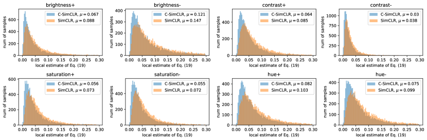
Figure 3: Histograms of Equation 19 (also Equation 28 in this section) on 10,000 training images. Each local estimate is Equation 28 with a $(x,x+\Delta x)$ pair. Here $x$ is the original image and $x+\Delta x$ is the augmented image. SimCLR is in orange. C-SimCLR is in blue. Higher $y$-axis values for lower $x$-axis values are better. We also report the mean ($\mu$) values. C-SimCLR consistently outperforms SimCLR.

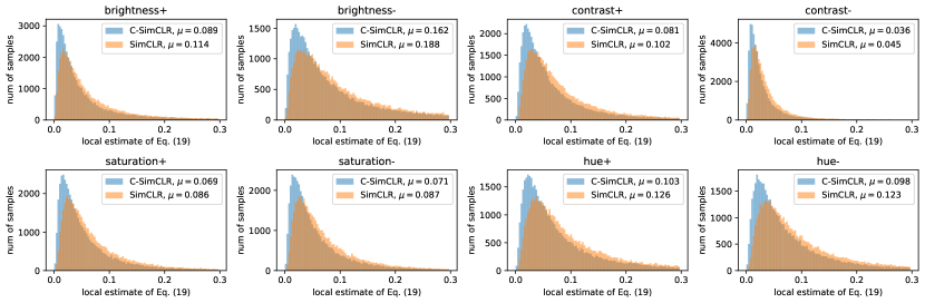
Figure 4: The same as Figure 3, but on 50,000 validation images.

Estimating the local Lipschitz constant.

We can evaluate Equation 19 (also Equation 28 on any $(x,x+\Delta x)$ pairs to estimate how smooth our model is at that point, and to compare the relative smoothness of different models. Here, we consider $(x,x+\Delta x)$ pairs where $x$ is taken either from the training or the validation set (using only a center crop in both cases), and $x+\Delta x$ is generated by either increasing or decreasing exactly one of: brightness, contrast, saturation, or hue. The absolute changes are the maximum adjustment strength in our image defined in Table 6 (e.g. for increasing brightness, we increase by 0.4). In Figures 3 and 4, we compare the histograms of Equation 19 on the SimCLR ResNet-50 model and the corresponding C-SimCLR ResNet-50 model. On both datasets and all eight augmentations, the C-SimCLR models have substantially more mass in the lower values of the local Lipschitz estimates for those image pairs, and have lower mean values computed over the dataset. Additionally, the mean C-SimCLR results on the validation set are almost all lower or equal to the mean SimCLR results on the training set, so the smoothness improvements from adding compression to SimCLR appear to be substantial. The only exceptions are for ‘brightness+’ (SimCLR training mean: 0.088, C-SimCLR validation mean: 0.089) and ‘brightness-’ (SimCLR training mean: 0.147, C-SimCLR validation mean: 0.162).

Appendix H Pseudocode

Listings 5 and 6 show Tensorflow pseudocode for C-SimCLR and C-BYOL respectively.

⬇

tfd = tensorflow_probability.distributions

\pardef simclr_ceb_loss(x,

y,

f_enc,

kappa_e=1024.0,

kappa_b=10.0,

beta=1.0):

"""Compute a Contrastive version of CEB loss for C-SimCLR model.

\parIn practice, we follow SimCLR to apply this loss in a bidirectional manner as

loss = simclr_ceb_loss(x, y) + simclr_ceb_loss(y, x).

We use the same notation as the main paper.

\parArgs:

x: An augmented image view. The expected shape is [B, H, W, C].

y: An augmented image view. The expected shape is [B, H, W, C].

f_enc: An image encoder (Conv + Projection in Fig. 1).

kappa_e: A float. Concentration parameter of distribution e.

kappa_b: A float. Concentration parameter of distribution b.

beta: CEB beta for controlling compression strength (Equation 1).

\parReturns:

A tensor ‘loss‘. The loss is per-sample.

"""

# Obtain unit-length mean direction vectors with expected shape [B, r_dim].

r_x = tf.math.l2_normalize(f_enc(x), -1)

r_y = tf.math.l2_normalize(f_enc(y), -1)

\parbatch_size = tf.shape(r_x)[0]

labels_idx = tf.range(batch_size)

# Labels are pseudo-labels which mark corresponding positives in a batch

labels = tf.one_hot(labels_idx, batch_size)

mi_upper_bound = tf.math.log(tf.cast(batch_size, tf.float32))

\pare_zx = tfd.VonMisesFisher(r_x, kappa_e)

b_zy = tfd.VonMisesFisher(r_y, kappa_b)

z = e_zx.sample()

log_e_zx = e_zx.log_prob(z)

log_b_zy = b_zy.log_prob(z)

i_xzy = log_e_zx - log_b_zy # residual information I(X;Z|Y)

logits_ab = b_zy.log_prob(z[:, None, :]) # broadcast

\par# The following categorical corresponds to c(y|z) and d(x|z) in Equation 12:

cat_dist_ab = tfd.Categorical(logits=logits_ab)

h_yz = -cat_dist_ab.log_prob(labels_idx)

i_yz = mi_upper_bound - h_yz

loss = beta * i_xzy - i_yz

\parreturn loss

Figure 5: Tensorflow pseudocode of C-SimCLR.

⬇

tfd = tensorflow_probability.distributions

\pardef byol_ceb_loss(x,

x_prime,

f_enc,

f_enc_target,

q_net,

l_net,

m_net,

kappa_e=16384.0,

kappa_b=10.0,

beta=1.0,

byol_loss_weight=2.0):

"""Compute loss for C-BYOL model.

\parThe notation corresponds to Section 2.3 and Figure 2 of the paper.

This code presents an updated version of C-BYOL as described in the

general response.

\parIn practice, we follow BYOL to apply this loss in a bidirectional manner as

loss = byol_ceb_loss(x, x_prime, …) + byol_ceb_loss(x_prime, x, …).

We use the same notation as the main paper.

\parArgs:

x: An augmented image view. The expected shape is [B, H, W, C].

x_prime: An augmented image view. The expected shape is [B, H, W, C].

f_enc: An image encoder (Conv + Projection in Fig. 2).

f_enc_target: The target image encoder. A slow moving-average of f_enc.

q_net: The BYOL predictor, which is a two-layer MLP.

l_net: A transformation function. We choose a linear layer in this work.

m_net: A transformation function. We choose a two-layer MLP in this work.

kappa_e: A float. Concentration parameter of distribution e.

kappa_b: A float. Concentration parameter of distribution b.

beta: CEB beta for controlling compression strength (Equation 1).

byol_loss_weight: BYOL loss weight. byol_loss_weight = kappa_d/2.

\parReturns:

A tensor ‘loss‘. The loss is per-sample.

"""

r = f_enc(x)

mu_e = tf.math.l2_normalize(q_net(r), -1)

e_zx = tfd.VonMisesFisher(mu_e, kappa_e)

z = e_zx.sample()

y_pred = tf.math.l2_normalize(l_net(z), -1)

\parr_t = tf.math.l2_normalize(f_enc_target(x), -1)

y = tf.stop_gradient(r_t)

mu_b = tf.math.l2_normalize(m_net(y), -1)

b_zy = tfd.VonMisesFisher(mu_b, kappa_b)

\parr_t_prime = tf.math.l2_normalize(f_enc_target(x_prime), -1)

y_prime = tf.stop_gradient(r_t_prime)

\par# byol_loss corresponds to -log d(y|z) as described in Section 2.3

byol_loss = tf.reduce_sum(tf.math.square(y_pred - y_prime), axis=-1)

\parlog_e_zx = e_zx.log_prob(z)

log_b_zy = b_zy.log_prob(z)

i_xzy = log_e_zx - log_b_zy

\parloss = byol_loss_weight * byol_loss + beta * i_xzy

\parreturn loss

Figure 6: Tensorflow pseudocode of C-BYOL.

References

- [1] Alessandro Achille and Stefano Soatto. Emergence of invariance and disentanglement in deep representations. The Journal of Machine Learning Research, 19(1):1947–1980, 2018.
- [2] Alessandro Achille and Stefano Soatto. Information dropout: Learning optimal representations through noisy computation. IEEE transactions on pattern analysis and machine intelligence, 40(12):2897–2905, 2018.
- [3] Alexander A Alemi, Ian Fischer, Joshua V Dillon, and Kevin Murphy. Deep variational information bottleneck. In International Conference on Learning Representations, 2017.
- [4] Philip Bachman, R Devon Hjelm, and William Buchwalter. Learning representations by maximizing mutual information across views. Advances in Neural Information Processing Systems, 32:15535–15545, 2019.
- [5] Andrei Barbu, David Mayo, Julian Alverio, William Luo, Christopher Wang, Dan Gutfreund, Josh Tenenbaum, and Boris Katz. ObjectNet: A large-scale bias-controlled dataset for pushing the limits of object recognition models. Advances in Neural Information Processing Systems, 32:9453–9463, 2019.
- [6] Thomas Berg, Jiongxin Liu, Seung Woo Lee, Michelle L Alexander, David W Jacobs, and Peter N Belhumeur. Birdsnap: Large-scale fine-grained visual categorization of birds. In Proceedings of the IEEE Conference on Computer Vision and Pattern Recognition, pages 2011–2018, 2014.
- [7] Lukas Bossard, Matthieu Guillaumin, and Luc Van Gool. Food-101–mining discriminative components with random forests. In European conference on computer vision, pages 446–461. Springer, 2014.
- [8] Glenn W Brier. Verification of forecasts expressed in terms of probability. Monthly weather review, 78(1):1–3, 1950.
- [9] Joan Bruna and Stéphane Mallat. Invariant scattering convolution networks. IEEE transactions on pattern analysis and machine intelligence, 35(8):1872–1886, 2013.
- [10] Mathilde Caron, Piotr Bojanowski, Armand Joulin, and Matthijs Douze. Deep clustering for unsupervised learning of visual features. In Proceedings of the European Conference on Computer Vision (ECCV), pages 132–149, 2018.
- [11] Mathilde Caron, Ishan Misra, Julien Mairal, Priya Goyal, Piotr Bojanowski, and Armand Joulin. Unsupervised learning of visual features by contrasting cluster assignments. arXiv preprint arXiv:2006.09882, 2020.
- [12] Ting Chen, Simon Kornblith, Mohammad Norouzi, and Geoffrey Hinton. A simple framework for contrastive learning of visual representations. In International conference on machine learning, pages 1597–1607. PMLR, 2020.
- [13] Ting Chen, Simon Kornblith, Kevin Swersky, Mohammad Norouzi, and Geoffrey E Hinton. Big self-supervised models are strong semi-supervised learners. Advances in Neural Information Processing Systems, 33:22243–22255, 2020.
- [14] Xinlei Chen, Haoqi Fan, Ross Girshick, and Kaiming He. Improved baselines with momentum contrastive learning. arXiv preprint arXiv:2003.04297, 2020.
- [15] Xinlei Chen and Kaiming He. Exploring simple siamese representation learning. In Proceedings of the IEEE/CVF Conference on Computer Vision and Pattern Recognition, pages 15750–15758, 2021.
- [16] Mircea Cimpoi, Subhransu Maji, Iasonas Kokkinos, Sammy Mohamed, and Andrea Vedaldi. Describing textures in the wild. In Proceedings of the IEEE Conference on Computer Vision and Pattern Recognition, pages 3606–3613, 2014.
- [17] Joshua V Dillon, Ian Langmore, Dustin Tran, Eugene Brevdo, Srinivas Vasudevan, Dave Moore, Brian Patton, Alex Alemi, Matt Hoffman, and Rif A Saurous. Tensorflow distributions. arXiv preprint arXiv:1711.10604, 2017.
- [18] Josip Djolonga, Frances Hubis, Matthias Minderer, Zachary Nado, Jeremy Nixon, Rob Romijnders, Dustin Tran, and Mario Lucic. Robustness Metrics, 2020. https://github.com/google-research/robustness_metrics.
- [19] Josip Djolonga, Jessica Yung, Michael Tschannen, Rob Romijnders, Lucas Beyer, Alexander Kolesnikov, Joan Puigcerver, Matthias Minderer, Alexander D’Amour, Dan Moldovan, et al. On robustness and transferability of convolutional neural networks. arXiv preprint arXiv:2007.08558, 2020.
- [20] Carl Doersch, Abhinav Gupta, and Alexei A Efros. Unsupervised visual representation learning by context prediction. In Proceedings of the IEEE international conference on computer vision, pages 1422–1430, 2015.
- [21] Yann Dubois, Benjamin Bloem-Reddy, Karen Ullrich, and Chris J Maddison. Lossy compression for lossless prediction. arXiv preprint arXiv:2106.10800, 2021.
- [22] Yann Dubois, Douwe Kiela, David J Schwab, and Ramakrishna Vedantam. Learning optimal representations with the decodable information bottleneck. In H. Larochelle, M. Ranzato, R. Hadsell, M. F. Balcan, and H. Lin, editors, Advances in Neural Information Processing Systems, volume 33, pages 18674–18690. Curran Associates, Inc., 2020.
- [23] Mahyar Fazlyab, Alexander Robey, Hamed Hassani, Manfred Morari, and George J Pappas. Efficient and accurate estimation of lipschitz constants for deep neural networks. NeurIPS, 2019.
- [24] Marco Federici, Anjan Dutta, Patrick Forré, Nate Kushman, and Zeynep Akata. Learning robust representations via multi-view information bottleneck. arXiv preprint arXiv:2002.07017, 2020.
- [25] Li Fei-Fei, Rob Fergus, and Pietro Perona. Learning generative visual models from few training examples: An incremental bayesian approach tested on 101 object categories. In 2004 conference on computer vision and pattern recognition workshop, pages 178–178. IEEE, 2004.
- [26] Ian Fischer. The conditional entropy bottleneck. Entropy, 22(9), 2020.
- [27] Ian Fischer and Alexander A. Alemi. Ceb improves model robustness. Entropy, 22(10), 2020.
- [28] Ian Goodfellow, Jean Pouget-Abadie, Mehdi Mirza, Bing Xu, David Warde-Farley, Sherjil Ozair, Aaron Courville, and Yoshua Bengio. Generative adversarial nets. Advances in neural information processing systems, 27, 2014.
- [29] Sven Gowal, Po-Sen Huang, Aaron van den Oord, Timothy Mann, and Pushmeet Kohli. Self-supervised adversarial robustness for the low-label, high-data regime. In International Conference on Learning Representations, 2021.
- [30] Jean-Bastien Grill, Florian Strub, Florent Altché, Corentin Tallec, Pierre H Richemond, Elena Buchatskaya, Carl Doersch, Bernardo Avila Pires, Zhaohan Daniel Guo, Mohammad Gheshlaghi Azar, et al. Bootstrap your own latent: A new approach to self-supervised learning. In Advances in Neural Information Processing Systems, volume 33, pages 21271–21284, 2020.
- [31] Zhaohan Daniel Guo, Bernardo Avila Pires, Bilal Piot, Jean-Bastien Grill, Florent Altché, Rémi Munos, and Mohammad Gheshlaghi Azar. Bootstrap latent-predictive representations for multitask reinforcement learning. In International Conference on Machine Learning, pages 3875–3886. PMLR, 2020.
- [32] Md Hasnat, Julien Bohné, Jonathan Milgram, Stéphane Gentric, and Liming Chen. von mises-fisher mixture model-based deep learning: Application to face verification. arXiv preprint arXiv:1706.04264, 2017.
- [33] Kaiming He, Haoqi Fan, Yuxin Wu, Saining Xie, and Ross Girshick. Momentum contrast for unsupervised visual representation learning. In Proceedings of the IEEE/CVF Conference on Computer Vision and Pattern Recognition, pages 9729–9738, 2020.
- [34] Kaiming He, Xiangyu Zhang, Shaoqing Ren, and Jian Sun. Deep residual learning for image recognition. In Proceedings of the IEEE conference on computer vision and pattern recognition, pages 770–778, 2016.
- [35] Olivier Henaff. Data-efficient image recognition with contrastive predictive coding. In International Conference on Machine Learning, pages 4182–4192. PMLR, 2020.
- [36] Dan Hendrycks, Steven Basart, Norman Mu, Saurav Kadavath, Frank Wang, Evan Dorundo, Rahul Desai, Tyler Zhu, Samyak Parajuli, Mike Guo, et al. The many faces of robustness: A critical analysis of out-of-distribution generalization. arXiv preprint arXiv:2006.16241, 2020.
- [37] Dan Hendrycks and Thomas Dietterich. Benchmarking neural network robustness to common corruptions and perturbations. ICLR, 2019.
- [38] Dan Hendrycks, Kevin Zhao, Steven Basart, Jacob Steinhardt, and Dawn Song. Natural adversarial examples. CVPR, 2021.
- [39] Geoffrey E Hinton, Simon Osindero, and Yee-Whye Teh. A fast learning algorithm for deep belief nets. Neural computation, 2006.
- [40] R Devon Hjelm, Alex Fedorov, Samuel Lavoie-Marchildon, Karan Grewal, Phil Bachman, Adam Trischler, and Yoshua Bengio. Learning deep representations by mutual information estimation and maximization. arXiv preprint arXiv:1808.06670, 2018.
- [41] Sergey Ioffe and Christian Szegedy. Batch normalization: Accelerating deep network training by reducing internal covariate shift. In International conference on machine learning, pages 448–456. PMLR, 2015.
- [42] Diederik P Kingma and Max Welling. Auto-encoding variational bayes. arXiv preprint arXiv:1312.6114, 2013.
- [43] Alexander Kolesnikov, Xiaohua Zhai, and Lucas Beyer. Revisiting self-supervised visual representation learning. In Proceedings of the IEEE/CVF Conference on Computer Vision and Pattern Recognition, pages 1920–1929, 2019.
- [44] Simon Kornblith, Jonathon Shlens, and Quoc V Le. Do better imagenet models transfer better? In Proceedings of the IEEE/CVF Conference on Computer Vision and Pattern Recognition, pages 2661–2671, 2019.
- [45] Jonathan Krause, Jia Deng, Michael Stark, and Li Fei-Fei. Collecting a large-scale dataset of fine-grained cars. In The 2nd Fine-Grained Visual Categorization Workshop, 2013.
- [46] Alex Krizhevsky. Learning multiple layers of features from tiny images. Technical report, Citeseer, 2009.
- [47] Kuang-Huei Lee, Ian Fischer, Anthony Liu, Yijie Guo, Honglak Lee, John Canny, and Sergio Guadarrama. Predictive information accelerates learning in RL. Advances in Neural Information Processing Systems, 33:11890–11901, 2020.
- [48] Junnan Li, Pan Zhou, Caiming Xiong, and Steven Hoi. Prototypical contrastive learning of unsupervised representations. In International Conference on Learning Representations, 2021.
- [49] Ilya Loshchilov and Frank Hutter. SGDR: Stochastic gradient descent with warm restarts. arXiv preprint arXiv:1608.03983, 2016.
- [50] Aleksander Madry, Aleksandar Makelov, Ludwig Schmidt, Dimitris Tsipras, and Adrian Vladu. Towards deep learning models resistant to adversarial attacks. arXiv preprint arXiv:1706.06083, 2017.
- [51] Subhransu Maji, Esa Rahtu, Juho Kannala, Matthew Blaschko, and Andrea Vedaldi. Fine-grained visual classification of aircraft. arXiv preprint arXiv:1306.5151, 2013.
- [52] Maria-Elena Nilsback and Andrew Zisserman. Automated flower classification over a large number of classes. In 2008 Sixth Indian Conference on Computer Vision, Graphics & Image Processing, pages 722–729. IEEE, 2008.
- [53] Mehdi Noroozi and Paolo Favaro. Unsupervised learning of visual representations by solving jigsaw puzzles. In ECCV, 2016.
- [54] Aaron van den Oord, Yazhe Li, and Oriol Vinyals. Representation learning with contrastive predictive coding. arXiv preprint arXiv:1807.03748, 2018.
- [55] Omkar M Parkhi, Andrea Vedaldi, Andrew Zisserman, and CV Jawahar. Cats and dogs. In 2012 IEEE conference on computer vision and pattern recognition, pages 3498–3505. IEEE, 2012.
- [56] Ben Poole, Sherjil Ozair, Aaron Van Den Oord, Alex Alemi, and George Tucker. On variational bounds of mutual information. In International Conference on Machine Learning, pages 5171–5180. PMLR, 2019.
- [57] Esteban Real, Jonathon Shlens, Stefano Mazzocchi, Xin Pan, and Vincent Vanhoucke. Youtube-boundingboxes: A large high-precision human-annotated data set for object detection in video. CVPR, 2017.
- [58] Benjamin Recht, Rebecca Roelofs, Ludwig Schmidt, and Vaishaal Shankar. Do ImageNet classifiers generalize to ImageNet? ICML, 2019.
- [59] Danilo Jimenez Rezende, Shakir Mohamed, and Daan Wierstra. Stochastic backpropagation and variational inference in deep latent gaussian models. In International Conference on Machine Learning, 2014.
- [60] Olga Russakovsky, Jia Deng, Hao Su, Jonathan Krause, Sanjeev Satheesh, Sean Ma, Zhiheng Huang, Andrej Karpathy, Aditya Khosla, Michael Bernstein, Alexander C. Berg, and Li Fei-Fei. ImageNet Large Scale Visual Recognition Challenge. International Journal of Computer Vision (IJCV), 2015.
- [61] Ohad Shamir, Sivan Sabato, and Naftali Tishby. Learning and generalization with the information bottleneck. In Yoav Freund, László Györfi, György Turán, and Thomas Zeugmann, editors, Algorithmic Learning Theory, pages 92–107. Springer Berlin Heidelberg, 2008.
- [62] Vaishaal Shankar, Achal Dave, Rebecca Roelofs, Deva Ramanan, Benjamin Recht, and Ludwig Schmidt. Do image classifiers generalize across time? arXiv preprint arXiv:1906.02168, 2019.
- [63] Karthik Sridharan and Sham M Kakade. An information theoretic framework for multi-view learning. In Proceedings of the 21st Annual Conference on Learning Theory, pages 403–414, 2008.
- [64] Yonglong Tian, Dilip Krishnan, and Phillip Isola. Contrastive multiview coding. arXiv preprint arXiv:1906.05849, 2019.
- [65] Yonglong Tian, Chen Sun, Ben Poole, Dilip Krishnan, Cordelia Schmid, and Phillip Isola. What makes for good views for contrastive learning. arXiv preprint arXiv:2005.10243, 2020.
- [66] Naftali Tishby, Fernando C Pereira, and William Bialek. The information bottleneck method. arXiv preprint physics/0004057, 2000.
- [67] Naftali Tishby and Noga Zaslavsky. Deep learning and the information bottleneck principle. In 2015 IEEE Information Theory Workshop (ITW), pages 1–5. IEEE, 2015.
- [68] Matías Vera, Pablo Piantanida, and Leonardo Rey Vega. The role of information complexity and randomization in representation learning. arXiv preprint arXiv:1802.05355, 2018.
- [69] Pascal Vincent, Hugo Larochelle, Yoshua Bengio, and Pierre-Antoine Manzagol. Extracting and composing robust features with denoising autoencoders. In Proceedings of the 25th international conference on Machine learning, pages 1096–1103, 2008.
- [70] Tongzhou Wang and Phillip Isola. Understanding contrastive representation learning through alignment and uniformity on the hypersphere. In International Conference on Machine Learning, pages 9929–9939. PMLR, 2020.
- [71] Tsui-Wei Weng, Huan Zhang, Pin-Yu Chen, Jinfeng Yi, Dong Su, Yupeng Gao, Cho-Jui Hsieh, and Luca Daniel. Evaluating the robustness of neural networks: An extreme value theory approach. In International Conference on Learning Representations, 2018.
- [72] Jianxiong Xiao, James Hays, Krista A Ehinger, Aude Oliva, and Antonio Torralba. Sun database: Large-scale scene recognition from abbey to zoo. In 2010 IEEE computer society conference on computer vision and pattern recognition, pages 3485–3492. IEEE, 2010.
- [73] Yao-Yuan Yang, Cyrus Rashtchian, Hongyang Zhang, Ruslan Salakhutdinov, and Kamalika Chaudhuri. A closer look at accuracy vs. robustness. Advances in Neural Information Processing Systems, 33, 2020.
- [74] Yang You, Igor Gitman, and Boris Ginsburg. Large batch training of convolutional networks. arXiv preprint arXiv:1708.03888, 2017.
- [75] Sergey Zagoruyko and Nikos Komodakis. Wide residual networks. arXiv preprint arXiv:1605.07146, 2016.
- [76] Jure Zbontar, Li Jing, Ishan Misra, Yann LeCun, and Stéphane Deny. Barlow twins: Self-supervised learning via redundancy reduction. arXiv preprint arXiv:2103.03230, 2021.
- [77] Xiaohua Zhai, Avital Oliver, Alexander Kolesnikov, and Lucas Beyer. S4L: Self-supervised semi-supervised learning. In Proceedings of the IEEE/CVF International Conference on Computer Vision, pages 1476–1485, 2019.