An Abelian Higgs model of pulsed field magnetization in superconductors

Abstract

Pulsed field magnetization leads to trapped magnetic field persistent for long times.We present a one-dimensional model of the interaction between an electromagnetic wave and a superconducting slab based on the Maxwell-Ginzburg-Landau (Abelian Higgs) theory. We first derive the model starting from a Lagrangian coupling the electromagnetic field with the Ginzburg-Landau potential for the superconductor. Then we explore numerically its capabilities by applying a Gaussian vector potential pulse and monitoring usual quantities such as the modulus and the phase of the order parameter. We also introduce defects in the computational domain. We show that the presence of defects enhances the remanent vector potential and diminishes the modulus of the order parameter, in agreement with existing experiments.

1 Introduction

High temperature superconductors have great advantages for energy applications because of their zero electrical resistance and relatively low cooling costs. Important devices are cryo-magnets capable to trap a large magnetic field inside a material cooled below a critical temperature. These systems have many applications such as Maglev trains, motors, wind-mills, etc. Figure 2 illustrates a Pulsed Field magnetization (PFM) setup where a cooled superconductor is submitted to a short pulse (a few $\mu$s) of magnetic field. Figure 2 shows a typical experimental result with a trapped field that is shown to last for days, even weeks [2].

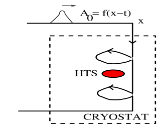
Figure 1: Pulse field magnetization experimental set up [10].

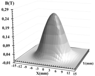
Figure 2: Magnetic cartography of trapped field ina GdBCO sample magnetised with the flux cooling method at CRISMAT (Caen, France).

This multi-physics aspect makes the problem difficult to tackle theoretically when flux motion, mechanical and thermal time scales are considered. To model PFM, a common pattern is to couple Maxwell’s equations, a constitutive law, the heat equation and the equations of elasticity [3]. This type of model permits to reproduce experimental results but does not allow to understand the micro/macroscopic mechanism that enables a superconductor to trap a magnetic field in a few milliseconds.

In this work, we address precisely this question. First, we note that Maxwell’s equations and the standard constitutive laws ($E/J$ power-law) cannot explain the presence of a stationary field after the passage of the applied electromagnetic pulse. Then, to refine the theoretical approach, we couple Maxwell’s equations for the vector potential with the Ginzburg-Landau equations. We keep the wave like character of the model (Lorentz invariance). This is the Abelian Higgs model.

We study a one-dimensional configuration where a superconducting slab is submitted to an electromagnetic pulse. We derive the equations of motion and interface conditions using a Lagrangian formalism. The numerical model deals with a pulse longer than the computational domain and absorbing boundary conditions. Numerical simulations show very little trapping in a clean sample without defects and important trapping when defects are present. In the latter case, we observe flux jumps.

The article is organized as follows: in section 2, we recall the constitutive equations used for modeling superconductors. In section 3 we introduce the idea of a non trivial fixed point of the system of equations. In section 4, we derive the equations for the one-dimensional system. In section 5 we present the numerical method and in section 6 we show the results.

2 The model

Consider Maxwell’s equations [5]

$$\nabla\cdot\mathbf{E}={\rho\over\epsilon_{0}},$$ (1)

$$\nabla\times\mathbf{E}=-\frac{\partial\mathbf{B}}{\partial t},$$ (2)

$$\nabla\cdot\mathbf{B}=0,$$ (3)

$$c^{2}\nabla\times\mathbf{B}={\mathbf{J}\over\epsilon_{0}}+\frac{\partial\mathbf{E}}{\partial t},$$ (4)

where $\mathbf{E},\mathbf{B}$ are the electric and magnetic fields, respectively. $\rho$ is a static charge density, $\mathbf{J}$ is the current (moving charge) density and $c$ is the velocity of light.

We model a superconducting material. Hence, no static charges are present and we assume $\rho=0$. We introduce the vector potential $\mathbf{A}$, such that

$$\mathbf{B}=\nabla\times\mathbf{A}.$$ (5)

Then Eq. (3) is satisfied and Eq. (2) implies

$$\mathbf{E}=-\frac{\partial\mathbf{A}}{\partial t}.$$ (6)

We also use the London gauge

$$\nabla\cdot\mathbf{A}=0.$$ (7)

Then, the last Maxwell equation (4) can be written as

$$\frac{\partial^{2}{\bf A}}{\partial t^{2}}-c^{2}\Delta\mathbf{A}={\mathbf{J}\over\epsilon_{0}}.$$ (8)

The main problem in this approach is to find an expression for $\mathbf{J}$. A first choice is the London approximation [7]:

$$\mathbf{J}=-{\epsilon_{0}c^{2}\over\lambda^{2}}\mathbf{A},$$ (9)

where $\lambda$ is the London characteristic length. Another expression, frequently used for large fields is a power law [1]

$$E=J^{n},$$ (10)

where $E$ is the amplitude of $\mathbf{E}$. This can be refined to obtain the Bean-Kim model [8]:

$$\mathbf{J}=\mathbf{J_{0}}{B\over B+B_{0}}\tanh({E\over E_{c}}),$$ (11)

where $B$ is the magnitude of $\mathbf{B}$ and $J_{0},B_{0},E_{c}$ are constants.

3 Existence of a non trivial fixed point

Experiments on magnetic flux jumps [10] report that there is a threshold of the applied magnetic field above which the sample switches from a transient to a permanent magnetization. In [10], the trapped field is presented as a function of the radius, for different applied fields $B$ from 1.44 T to 2.69 T, and shows a clear jump for $B>1.57$ T. The trapped field thus produced is observed to remain stable for very long times, much longer than the duration of the initial pulse. This indicates that the system switches from one type of state close to zero to another non-nul state. Dynamically, this means that there should exists a non trivial fixed point in the coupled equations (8),(9) or (8), (11).

Equations (8) and (9), or (8) and (11), do not support non trivial fixed points. This is straightforward to obtain for (9). For (11), we rewrite the system (8),(11) using (5) and (7)

$$\displaystyle\frac{\partial\mathbf{A}}{\partial t}=\mathbf{C},$$ (12)

$$\displaystyle\frac{\partial\mathbf{C}}{\partial t}=c^{2}\Delta\mathbf{A}-{1\over\epsilon_{0}}\mathbf{J_{0}}{B\over B+B_{0}}\tanh({\parallel\frac{\partial\mathbf{A}}{\partial t}\parallel\over E_{c}}),$$ (13)

where $\mathbf{C}$ is an auxiliary vector. Assume all quantities are scalars. When searching a fixed point, we assume $\displaystyle\frac{\partial{A}}{\partial t}=\frac{\partial{C}}{\partial t}=0$ and find that the only existing solution is $A=0$.

The conclusion of this simple analysis is that the constitutive equations (9),(10),(11) do not explain why a trapped field remains after the passage of the pulse. To address this issue, we start from first principles and use the full Ginzburg-Landau functional to describe the superconductor.

4 The Maxwell-Ginzburg-Landau model

As assumed above, the electromagnetic component of the problem is described by the vector potential. The superconductivity is represented by the complex order parameter $\psi$. The Ginzburg-Landau free energy in SI units can be written as [6]

$$F(\mathbf{A},\psi)=-\alpha|\psi|^{2}+{\beta\over 2}|\psi|^{4}+{1\over 4m}|(i\hbar\nabla+{2e}\mathbf{A})\psi|^{2},$$ (14)

where $m$ is the electron mass and $e$ is the electron charge. The $\alpha$ coefficient is usually taken as $\alpha_{0}(T-T_{c})$ where $\alpha_{0}>0$; here we assume $T<T_{c}$ so we use $-\alpha$.

Most studies of time dependent superconductivity assume that the system relaxes to an equilibrium. The dynamics is typically of gradient type. The effect we are describing takes the system out of equilibrium, hence we need a relativistic extension of the theory of superconductivity. This is provided by the Abelian Higgs model [15].

For simplicity, we start with a one-dimensional formulation of the problem. In the spirit of the study [11], we write a Lagrangian for Maxwell’s equations for the single component $A$ of the vector potential and the Ginzburg-Landau potential

$${\cal L}(A,\frac{\partial A}{\partial t},\frac{\partial A}{\partial x},\psi,\frac{\partial\psi}{\partial t},\frac{\partial\psi}{\partial x})=\frac{1}{2\mu_{0}c^{2}}\left(\frac{\partial A}{\partial t}\right)^{2}-\frac{1}{2\mu_{0}}\left(\frac{\partial A}{\partial x}\right)^{2}+I(x)\left[\alpha|\psi|^{2}-{\beta\over 2}|\psi|^{4}\right.$$

$$\left.+\frac{\hbar^{2}}{4mc^{2}}\left|\frac{\partial\psi}{\partial t}\right|^{2}-{1\over 4m}|(i\hbar\nabla+2eA)\psi|^{2}\right],$$ (15)

where $I(x)$ is the indicator function of the superconductor. We introduced a time dependence of $\psi$ following the Abelian Higgs model [15]. We use the subscripts ${}_{t},_{x}$ to indicate partial derivatives. The $|\frac{\partial\psi}{\partial t}|^{2}$ term corresponds to a relativistic generalization of the Ginzburg-Landau theory of superconductors. It describes a fast and out of equilibrium rearrangement of the order parameter.

We introduce the characteristic lengths $\xi,~{}\lambda$ and their ratio $\kappa$

$$\xi^{2}={\hbar^{2}\over 4m\alpha},~{}~{}~{}~{}\lambda^{2}={m\beta\over 2e^{2}\mu_{0}\alpha},~{}~{}\kappa={\lambda\over\xi}.$$ (16)

Following [12] we normalize the main variables as

$$x=\lambda x^{\prime},~{}~{}t={\lambda\over c}t^{\prime},~{}~{}\psi=\sqrt{\alpha\over\beta}\psi^{\prime},~{}~{}A={\hbar\over 2e\xi}A^{\prime}.$$ (17)

Plugging these expressions into the Lagrangian ${\cal L}$, we obtain

$${\cal L}=\left(\frac{\partial A}{\partial t}\right)^{2}-\left(\frac{\partial A}{\partial x}\right)^{2}+I(x)\left[{1\over\kappa^{2}}\left|\frac{\partial\psi}{\partial t}\right|^{2}-{1\over\kappa^{2}}\left|\frac{\partial\psi}{\partial x}\right|^{2}+i{1\over\kappa}A\left(\psi\frac{\partial\psi^{*}}{\partial x}-\psi^{*}\frac{\partial\psi}{\partial x}\right)\right.$$

$$\left.+|\psi|^{2}(1-A^{2})-{1\over 2}|\psi|^{4}\right].$$ (18)

The Euler-Lagrange equations yield the final system including the coupling conditions at interfaces $x=\pm L$ (see details in A)

$$\frac{\partial^{2}A}{\partial t^{2}}-\frac{\partial^{2}A}{\partial x^{2}}=I(x)\left[i{1\over 2\kappa}\left(\psi\frac{\partial\psi^{*}}{\partial x}-\psi^{*}\frac{\partial\psi}{\partial x}\right)-A|\psi|^{2}\right],$$ (19)

$$\frac{\partial^{2}\psi}{\partial t^{2}}-\frac{\partial^{2}\psi}{\partial x^{2}}=-{i\kappa}\left(\frac{\partial A}{\partial x}\psi+2A\frac{\partial\psi}{\partial x}\right)+\kappa^{2}\psi(1-|\psi|^{2}-A^{2})=0,~{}~{}~{}x\in[-L,L],$$ (20)

$$-iA\psi+{1\over\kappa}\frac{\partial\psi}{\partial x}=0,~{}~{}~{}x=\pm L.$$ (21)

Note that the scale of variation of $\psi$ is $1/\kappa$. For large values of $\kappa$ giant vortex states are expected [14].

5 Numerical model

Partial differential equations (19),(20) were solved using an ODE solver for the time advancement and finite differences for the space discretization.

We study how an electromagnetic pulse scatters off a superconducting layer. It is therefore important to prevent any out-going wave to bounce off the edge of the computational domain and interact again with the layer. To prevent this effect, we use absorbing boundary conditions $\displaystyle\frac{\partial A}{\partial t}=-\frac{\partial A}{\partial x},~{}~{}\frac{\partial A}{\partial t}=\frac{\partial A}{\partial x}$ at the left and right sides of the computational domain, respectively (see Fig. 3).

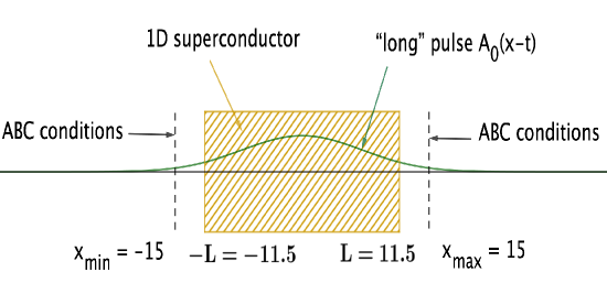
Figure 3: Schematics of the computational domain.

5.1 Defects

To trap magnetic flux inside the superconductor, we also study the effect of including defects in the model. We speculate that in the superconductor without defects, as soon as the field recedes, the order parameter returns to its original value and cannot sustain any long term magnetization.

Defects can be geometrically modelled as a wedge placed at the surface of the superconducting sample [12]. This is adapted to a 2D modeling of the sample and such a geometrical defect favors the penetration of vortices inside the sample. Another type of defect is a material inhomogeneity where the superconductivity breaks down at specific locations inside the slab. In practice, this can be obtained by bombarding the sample with heavy ions [10]. Our one-dimensional model then incorporates a function $s(x)$ in the $\alpha$ term of the free energy (14). This term varies from 1 (superconducting) to -1 (non superconducting), as in [13].

The precise form of the defect is

$$s(x)=\sum_{i=1}^{n_{d}}H(x-ix_{d}),$$ (22)

where $H$ is the square function $H(\xi)=-1$ if $\xi\in[-{w_{d}\over 2},{w_{d}\over 2}]$, $H(\xi)=1$ otherwise.

The equations including this type of defect are

$$\frac{\partial^{2}A}{\partial t^{2}}-\frac{\partial^{2}A}{\partial x^{2}}=I(x)\left[i{1\over 2\kappa}\left(\psi\frac{\partial\psi^{*}}{\partial x}-\psi^{*}\frac{\partial\psi}{\partial x}\right)-A|\psi|^{2}\right],$$ (23)

$$\frac{\partial^{2}\psi}{\partial t^{2}}-\frac{\partial^{2}\psi}{\partial x^{2}}=-{i\kappa}\left(\frac{\partial A}{\partial x}\psi+2A\frac{\partial\psi}{\partial x}\right)+\kappa^{2}\psi\left(s(x)-|\psi|^{2}-A^{2}\right),$$ (24)

$$-iA\psi+{1\over\kappa}\frac{\partial\psi}{\partial x}=0,~{}~{}~{}x=\pm L.$$ (25)

To model a pulse $A_{0}$ longer than the computational domain, we use the following transformation:

$$A=A^{\prime}+A_{0}(x-t),$$ (26)

where $\displaystyle A_{0}(x)=a_{0}\exp(-\frac{x^{2}}{2w_{0}})$. Since $A_{0}(x-t)$ satisfies the wave equation with speed $c=1$, Eqs. (23) and (24) become

$$\frac{\partial^{2}A^{\prime}}{\partial t^{2}}-\frac{\partial^{2}A^{\prime}}{\partial x^{2}}=I(x)\left[i{1\over 2\kappa}\left(\psi\frac{\partial\psi^{*}}{\partial x}-\psi^{*}\frac{\partial\psi}{\partial x}\right)-(A^{\prime}+A_{0})|\psi|^{2}\right],$$ (27)

$$\frac{\partial^{2}\psi}{\partial t^{2}}-\frac{\partial^{2}\psi}{\partial x^{2}}=-{i\kappa}\left(\frac{\partial A^{\prime}}{\partial x}\psi+2(A^{\prime}+A_{0})\frac{\partial\psi}{\partial x}\right)+\kappa^{2}\psi\left(s(x)-|\psi|^{2}-(A^{\prime}+A_{0})^{2}\right),$$ (28)

$$-i(A^{\prime}+A_{0})\psi+{1\over\kappa}\frac{\partial\psi}{\partial x}=0,~{}~{}~{}x=\pm L.$$ (29)

6 Numerical results

In all the runs presented in this section, the computational domain is $[-15,15]$ and the superconductor extent is $[-11.5,11.5]$. The time step is $dt=10^{-3}$ and the space step $dx=7.69~{}10^{-3}$. Most runs were performed with pulses hitting the slab from both directions. The typical pulse position and width are $x_{0}=-200$ and $w=50$, respectively.

6.1 Modulus and phase

A preliminary analysis of equations could be useful to understand numerical results. To this purpose we write the equations using modulus and phase of $\psi$:

$$\psi=\rho e^{i\theta}.$$ (30)

Then Eqs. (19)-(20) become

$$\frac{\partial^{2}A}{\partial t^{2}}-\frac{\partial^{2}A}{\partial x^{2}}=I(x)\rho^{2}\left(\frac{1}{\kappa}\frac{\partial\theta}{\partial x}-A\right),$$ (31)

$$\frac{\partial^{2}\rho}{\partial t^{2}}-\frac{\partial^{2}\rho}{\partial x^{2}}=\rho\left(\left(\frac{\partial\theta}{\partial t}\right)^{2}-\left(\frac{\partial\theta}{\partial x}\right)^{2}\right)+{2\kappa}A\rho\frac{\partial\theta}{\partial x}+\kappa^{2}\rho(1-\rho^{2}-A^{2}),$$ (32)

$$\frac{\partial^{2}\theta}{\partial t^{2}}-\frac{\partial^{2}\theta}{\partial x^{2}}={2\over\rho}\left(\frac{\partial\theta}{\partial x}\frac{\partial\rho}{\partial x}-\frac{\partial\theta}{\partial t}\frac{\partial\rho}{\partial t}\right)-\kappa\frac{\partial A}{\partial x}-2\kappa A\frac{1}{\rho}\frac{\partial\rho}{\partial x}.$$ (33)

The interface condition at $x=\pm L$ is

$$\frac{\partial\rho}{\partial x}=0,~{}~{}~{}\frac{\partial\theta}{\partial x}=\kappa A.$$ (34)

When analysing the system (31), (32), (33) we notice that a first approximation of the trapped field is $\frac{\partial\theta}{\partial x}=\kappa A\neq 0$. The corresponding full solution is

$$A=A_{\infty},~{}~{}\rho=1,~{}~{}\frac{\partial\theta}{\partial x}=\kappa A_{\infty}.$$ (35)

6.2 Effect of amplitude $a_{0}$

Figure 4 shows the time evolution of the averaged $A$ inside the superconducting strip for $a_{0}=0.2,~{}1,~{}3$ and 10. One notes that the trapped $A$ is very small for large amplitudes, $a_{0}=3$.

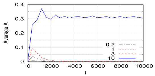
Figure 4: Time evolution of the averaged $A$ inside the superconducting strip for four amplitudes of the applied pulse: $a_{0}=0.2,~{}1,~{}3$ and 10.

Therefore to trap $A$ we need defects that will lock the phase.

6.3 Influence of defects

Figure 5 shows snapshots of the modulus and phase of $\psi(x,t)$ for $t=4416,4608$ and $4800$ for an incident pulse of amplitude $a_{0}=0.2$, with defects spaced by 0.05 and without defects. The left panel shows the modulus of the order parameter $\rho(x,t)$ for both cases.

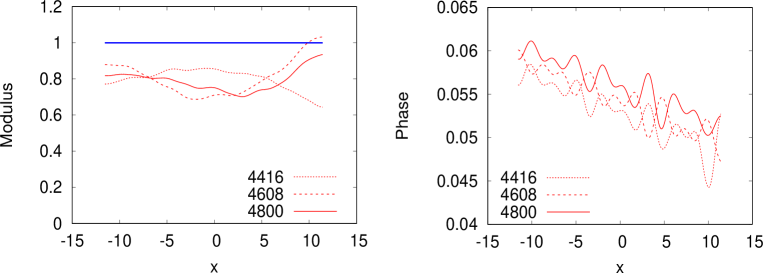
Figure 5: Snapshots of the modulus $\rho(x,t)$ (left panel) and the phase $\theta(x,t)$ (right panel) for $t=4416,4608$ and $4800$. The incident pulse has amplitude $a_{0}=0.2$.

Note that without defects $\rho$ equals one (continuous line, blue online) and does not evolve. Similarly, the phase $\theta$ remains flat at 0.

Figure 6 shows the importance of defects to obtain a non-zero vector potential.

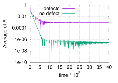
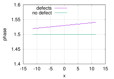
Figure 6: Time evolution of the averaged $A$ (left) and the phase $\theta$ (right) considering the presence or the absence of defects.

6.4 Influence of defect spacing

Figure 7 shows the influence of the density of defects on the modulus of the order parameter. More precisely, the average of $|\psi|$ both on space range $[-L,L]$ and time range $[0,40000]$ is a decreasing function of the density of defects. We defined this density as the ratio between the number of nodes where $s(x)=-1$ and the ones where $s(x)=+1$.

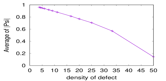
Figure 7: Space and time average of $|\psi|$ as a function of the density of defects (%).

In Fig. 8 the phase gradient and trapped $A$ are approximately $3\cdot 10^{-3}$ for $x_{d}=0.05$, while they raise to values around $1.8$ for $x_{d}=0.01$. Moreover, $\displaystyle\frac{\partial\theta}{\partial x}$ is negative for $x_{d}=0.05$ and positive for $x_{d}=0.01$. In addition $\rho(x,t)$ for $x_{d}=0.01$ becomes rather small and seems to oscillate periodically.

7 Conclusion

We presented a one-dimensional model describing the interaction of an electromagnetic pulse with a superconducting slab; it is based on the Abelian Higgs model. The novelty of this approach is to introduce second time derivatives in the equations for both vector potential and order parameter. The main features of our numerical method are the use of absorbing boundary conditions and an applied pulse whose support is longer than the computational domain.

The equations of motion and boundary conditions are derived from a Lagrangian via Euler-Lagrange equations. Numerical results indicate that the absence of defect leads to a vector potential close to zero. Moreover, the space and time average of the modulus of the order parameter is a decreasing function of the density of defects: this is consistent with the fact that defects reduce superconductivity by pinning vortices and, as a consequence, lower the modulus of the order parameter.

In conclusion, using this one-dimensional model, we retrieve the usual behaviour of superconductors. Future work will consider 2D configurations.

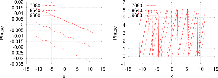
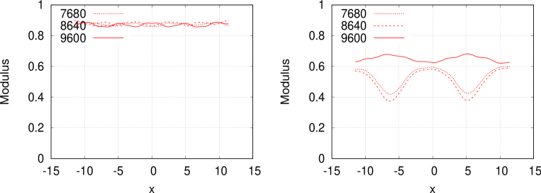
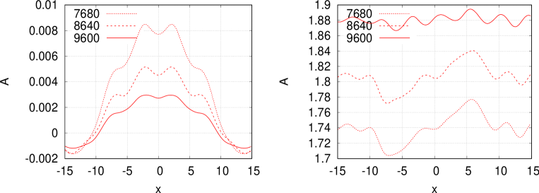
Figure 8: Snapshots of the phase $\theta(x,t)$ (top), modulus $\rho(x,t)$ (middle) and $A(x,t)$ (bottom) for $t=7680,8640$ and 9600 for a defect spacing $x_{d}=0.05$ (left panels) and $0.01$ (right panels). The incident pulse has an amplitude $a_{0}=3$ and the defect spacing is $w_{d}=10^{-3}$.

Acknowledgements
The present work was performed using computing resources of CRIANN (Normandy, France). The authors thank Nikos Flytzanis, Michikazu Kobayashi and Mads Peter Soerensen for useful comments. They also thank Pierre Bernstein and Jacques Noudem for sharing their experimental results.

Appendix A Evolution equations and boundary conditions

The Euler-Lagrange equations are

$$\frac{\partial}{\partial t}\left({\partial{\cal L}\over\partial\frac{\partial A}{\partial t}}\right)+\frac{\partial}{\partial x}\left({\partial{\cal L}\over\partial\frac{\partial A}{\partial x}}\right)-{\partial{\cal L}\over\partial A}=0,$$

$$\frac{\partial}{\partial t}\left({\partial{\cal L}\over\partial\frac{\partial\psi^{*}}{\partial t}}\right)+\frac{\partial}{\partial x}\left({\partial{\cal L}\over\partial\frac{\partial\psi^{*}}{\partial x}}\right)-{\partial{\cal L}\over\partial\psi^{*}}=0.$$

The equation for $A$ is

$$\frac{\partial^{2}A}{\partial t^{2}}-\frac{\partial^{2}A}{\partial x^{2}}=I(x)\left[i{1\over 2\kappa}\left(\psi\frac{\partial\psi^{*}}{\partial x}-\psi^{*}\frac{\partial\psi}{\partial x}\right)-A|\psi|^{2}\right].$$ (36)

For $\psi$ we obtain

$$\begin{array}[]{ll}\displaystyle I(x)\left[-{1\over\kappa^{2}}\frac{\partial^{2}\psi}{\partial t^{2}}+{1\over\kappa^{2}}\frac{\partial^{2}\psi}{\partial x^{2}}-{i\over\kappa}\left(\frac{\partial A}{\partial x}\psi+2A\frac{\partial\psi}{\partial x}\right)+\psi(1-|\psi|^{2}-A^{2})\right]\\ \displaystyle+\delta(x)\left(-{i\over\kappa}A\psi+{1\over\kappa^{2}}\frac{\partial\psi}{\partial x}\right)=0,\end{array}$$ (37)

where $\delta(x)$ is the Dirac distribution corresponding to the $x$ derivative of the characteristic function $I(x)$.

To obtain boundary conditions we integrate (36) over one of the edges of the domain. For example, for $x=-L$ we obtain

$$\int_{-L-\epsilon}^{-L+\epsilon}\frac{\partial^{2}A}{\partial t^{2}}-\left[{\frac{\partial A}{\partial x}}\right]_{-L-\epsilon}^{-L+\epsilon}=\int_{-L}^{-L+\epsilon}\left[i{1\over 2\kappa}\left(\psi\frac{\partial\psi^{*}}{\partial x}-\psi^{*}\psi_{x}\right)-A|\psi|^{2}\right].$$

Taking the limit $\epsilon\to 0$ and assuming bounded variations of the integrands, we obtain that $\frac{\partial A}{\partial x}$ is continuous at the interface $x=-L$. The second equation gives

$$\int_{-L}^{-L+\epsilon}\left[-{1\over\kappa^{2}}\frac{\partial^{2}\psi}{\partial t^{2}}+{1\over\kappa^{2}}\frac{\partial^{2}\psi}{\partial x^{2}}+\dots\right]+\left(-{i\over\kappa}A\psi+{1\over\kappa^{2}}\frac{\partial\psi}{\partial x}\right)_{x=-L}=0.$$

Taking the limit $\epsilon\to 0$ and assuming the bracket in the integral is bounded, we recover the following standard boundary condition [7] at the edge of a superconductor:

$$-iA\psi+{1\over\kappa}\frac{\partial\psi}{\partial x}=0.$$ (38)

References

[1]
J. Rhyner, Magnetic properties and AC-losses of superconductors with power law current—voltage characteristics, Physica C: Superconductivity
212, 3–4, 292-300, (1993).
[2]
D. Zhou, J. Srpcic, K. Huang, M. Ainslie, Y. Shi, A. Dennis, M. Boll, M. Filipenko, D. Cardwell and J. Durrell,
Reliable 4.8 T trapped magnetic fields in Gd–Ba–Cu–O bulk superconductors
using pulsed field magnetization
Supercond. Sci. Technol. 34, 034002, (2021).
[3] M. Ainslie et al. Supercond. Sci. Technol., 29, 074003,
(2016).
[4]
J.-G. Caputo, L. Gozzelino, F.Laviano, G.Ghigo, R.Gerbaldo, J.Noudem, Y.Thimont, P.Bernstein,
”Screening magnetic fields by a superconducting disk: a simple model”,
J. Appl. Phys. 114, 233913 (2013).
[5] R. Feynman, course of physics, Electromagnetism.
[6] M. Tinkham, ”Introduction to Superconductivity”, second edition, Dover, (2004).
[7] T. Van Duzer and C. W. Turner, ”Principles of superconductive devices and circuits”, Edward Arnold, (1998).
[8] C.P. Bean, Rev. Mod. Phys. 36, 31 (1964).
[9] M. Brio, J.G. Caputo, K. Gwirtz, J. Liu and A. Maimistov,
” Scattering of a short electromagnetic pulse from a Lorentz-Duffing film: theoretical and numerical analysis”,
Wave motion, 89, 43-56, (2019).
[10] R.Weinstein et al. IEEE Transactions on Applied
Superconductivity 25 , 6601106 (2014)
[11] J.-G. Caputo, E. V. Kazantseva, A.I. Maimistov,
”Electromagnetically induced switching of ferroelectric thin films”,
Phys. Rev. B 75, 014113 (2007).
[12] Alstrom, T. S., Sorensen, M. P., Pedersen, N. F., and Madsen, S. (2010). Magnetic Flux Lines in Complex
Geometry Type-II Superconductors Studied by the Time Dependent Ginzburg-Landau Equation. Acta
Applicandae Mathematicae, 115(1), 63-74.
[13] M. P. Sorensen, N. F. Pedersen,
The dynamics of magnetic vortices in type II superconductors with
pinning sites studied by the time dependent Ginzburg–Landau model
Physica C: Superconductivity and its applications, 533, 40–43, (2017).
[14] L.C. Garcia and J. Giraldo,
Giant vortex state in mesoscopic superconductors, Phys. Stat. Sol. (c) 2,
3609–3612, (2005).
[15] H. B. Nielsen and P. Olesen,
Nuclear Physics B61 (1973) 45-61. North-Holland Publishing Company