An A Quadcopter Autopilot Based on an Adaptive Digital PID Controller

Adaptive Digital PID Control of a Quadcopter

Retrospective-Cost-Based Adaptive Digital PID Control of a Quadcopter

A Retrospective-Cost-Based Adaptive Digital PID Quadcopter Autopilot

Adaptive Digital PID Control of a Quadcopter with Unknown Dynamics

One-Shot Learning for a Quadcopter Autopilot

An adaptive digital autopilot for Multicopters

Experimental Implementation of an Adaptive Digital Autopilot

An Adaptive PID Autotuner for Multicopters
with Experimental Results

Abstract

This paper develops an adaptive PID autotuner for multicopters, and presents simulation and experimental results. The autotuner consists of adaptive digital control laws based on retrospective cost adaptive control implemented in the PX4 flight stack. A learning trajectory is used to optimize the autopilot during a single flight. The autotuned autopilot is then compared with the default PX4 autopilot by flying a test trajectory constructed using the second-order Hilbert curve. In order to investigate the sensitivity of the autotuner to the quadcopter dynamics, the mass of the quadcopter is varied, and the performance of the autotuned and default autopilot is compared. It is observed that the autotuned autopilot outperforms the default autopilot.

I Introduction

Unmanned aerial vehicles, especially multicopters, have been used in a myriad of applications over the last decade, such as environment mapping, asset monitoring, risk assessment, sports broadcasting, wind-turbine inspection, and their applications continue to grow [1, 2, 3, 4, 5, 6]. In its most common form, a multicopter has four propellers. By controlling the spin rates of the four propellers, a force along a body-fixed axis and moments about three linearly independent body-fixed axes can be independently applied to affect desired translational as well as rotational motions. However, due to the nonlinear and unstable nature of the quadcopter dynamics, precise control of a quadcopter is a well-recognized challenging problem.

Nonlinear techniques such as feedback-linearization [7] and back-stepping [8] have been applied to deal with the nonlinearities and to construct stabilizing controllers. However, these techniques require accurate plant models at all operating conditions [9]. Adaptive techniques have also been investigated to reduce the need for an accurate model [10, 11], however, they also require a sufficiently accurate plant model to construct stabilizing controllers. Iterative learning control is used learn the pitch and roll controller in the closed-loop system in [12]. Reinforcement learning control is used to learn low-level controllers in case of multiple actuator failure in [13]. L1 adaptive control is used to improve the stability margins of a stable control loop in a quadcopter flight control system in [14]. Fuzzy control was used in the position control in [15]. Bidirectional brain emotional learning was used to improve trajectory tracking and handle payload uncertainties in [16]. Model reference adaptive control was used in the attitude controller in [17] to counteract model uncertainties. Adaptive twisting sliding mode control was used in the attitude controller in [18] to resolve the chattering issues in standard sliding mode control. Robust fixed point transformation based adaptive control was used in [19] to improve quadcopter stability in the presence of parameter uncertainties and external disturbances. Adaptive particle swarm optimization was used in a PD controller (APSO-PD) in [20] to improve the rise time, settling time, overshoot, and peak time of a standard PSO controller. Robust adaptive control based on backstepping is used in [21] [22] to provide robust quadcopter altitude and attitude tracking after payload change. Immersion and invariance based adaptive backstepping control is used in [23] to remedy quadcopter attitude instabilities due to disturbance torques or parameter uncertainties. Adaptive fault tolerant control based on the adaptive minimum projection method is used to provide quadcopter stability in the event of actuator failure in [24]. Balanced control is used in [25] to improve quadcopter performance by switching between fuzzy adaptive PID and optimized PID midflight. L1 adaptive control is used in [26] to stabilize a fixed-wing pitch controller, and in [27] to counteract fixed-wing split drag rudder damage. Adaptive control is also used in [28] to resolve instabilities due to trailing vortices in fixed-wing formation flight. Online adaptive model parameter estimation is used in the velocity controller in [29] to mitigate error due to model parameter uncertainty. However, most of these control techniques focus on optimizing a part of the control system, assuming that the rest of the control system is sufficiently good.

Typical quadcopter autopilots are, however, based on cascaded controllers, which consist of an inner loop to stabilize the dynamics, and an outer loop to track position commands. Traditionally, all controllers in the autopilot are constructed using manually tuned PID control laws. In fact, widely used open-source autopilots such as PX4 and ArduPilot contain finely-tuned PID control laws for many commercially available multicopter configurations [30, 31]. These autopilots cannot guarantee stability and thus have a fixed operational envelope, which is usually unknown. Moreover, autopilots tuned for a specific geometry and inertia properties do not perform well in the case where these properties vary with time, such as, in the case of unknown suspended payload, hardware alteration, and dynamic environmental changes. Such variations invariably degrade the performance of the autopilot.

With these motivations in mind, this paper develops an adaptive autotuner for multicopters with unknown dynamics. In particular, all of the fixed-gain control laws of an autopilot are replaced by adaptive control laws that optimize the gain by flying a single learning trajectory. Specifically, the adaptive controllers are updated by the retrospective cost adaptive control (RCAC) algorithm [32]. The learning trajectory is designed such that all possible motions of the quadcopter are excited and thus nonzero control outputs are required from all control laws, which ensures that all of the controller gains are adaptively updated.

The contribution of the work presented in this paper is the development of an adaptive autotuner that does not require any prior knowledge of the system dynamics, and instead uses a simple learning trajectory to adapt the autopilot gains; and its numerical and experimental demonstration. The performance of the autotuner is demonstrated by flying a test trajectory and comparing its performance with a finely-tuned autopilot. The improvements due to the autotuning process are demonstrated through simulations and flight tests.

The paper is organized as follows. Section II briefly presents the control system architecture implemented in the PX4 autopilot. Section III explains the setup of the adaptive autotuner. Section IV describes the RCAC algorithm used to tune the control parameters. Section V presents simulation and flight test results showing the adaptation of the autotuner and comparing the performance of the PX4 autopilot using the stock and autotuned control parameters. Finally, section VI concludes the paper with a summary and future research directions.

II Quadcopter Autopilot

This section reviews the quadcopter autopilot considered in this work. This autopilot is based on the control architecture implemented in the PX4 autopilot. The notation used in this paper is described in more detail in [33].

The control system consists of a mission planner and two nested loops as shown in Figure 1. The mission planner generates the position, velocity, and azimuth setpoints from the user-defined waypoints using the guidance law described below. The outer loop consists of the position controller, whose inputs are the position and velocity errors, defined as the difference between the setpoints and the measurements. The output of the position controller is the thrust vector setpoint. Note that the thrust vector is expressed in terms of the Earth-fixed frame. The inner loop consists of the attitude controller, whose inputs are the thrust vector setpoint, the azimuth and azimuth-rate setpoints, as well as the attitude and the angular rate measured in the body-fixed frame. The output of the attitude controller is the moment vector setpoint in the body-fixed frame. The magnitude of the thrust vector setpoint and the moment vector setpoint uniquely determine the required rotation rates of the four propellers.

Figure 1: Control-system architecture.

The mission planner uses a guidance law described in Appendix A to generate the position and the azimuth setpoints. Using a user-specified maximum velocity $v_{\rm max}$ and maximum acceleration $a_{\rm max}$, the guidance law generates a trajectory that consists of a constant acceleration phase, a cruise phase, and a constant deceleration phase. A similar guidance law is used to generate azimuth setpoints, given a user-specified maximum angular velocity $\dot{\psi}_{\rm max}$ and maximum angular acceleration $\ddot{\psi}_{\rm max}.$

The position controller consists of two cascaded linear controllers as shown in Figure 2. The first controller $G_{r}$ consists of three proportional controllers. The second controller $G_{v}$ consists of three decoupled PID controllers and a velocity setpoint feedforward controller, and yields the thrust vector setpoint.

Figure 2: Position controller architecture.

The force vector setpoint along with the azimuth setpoint are used to calculate the attitude setpoint, which is represented as a quaternion. The attitude controller consists of two cascaded controllers $G_{q}$ and $G_{\omega}$ as shown in Figure 3. The first controller $G_{q}$ is an almost globally stabilizing controller [34] that consists of three proportional gains. The second controller $G_{\omega}$ consists of three PID controllers and an angular rate setpoint feedforward controller, and yields the moment vector setpoint.

Figure 3: Attitude controller architecture.

The control system implemented in the PX4 autopilot thus consists of 27 gains. In particular, the outer loop includes three gains in $G_{r}$ and nine gains in $G_{v}$; and the inner loop includes three gains in $G_{q}$ and 12 gains in $G_{\omega}.$ In standard practice, these 27 gains are manually tuned and require considerable expertise.

III Adaptive Autotuner

The adaptive autotuner is constructed by replacing the fixed-gain controllers in the autopilot described in the previous section with adaptive controllers that are updated by retrospective cost optimization. In particular, each fixed-gain controller described in the previous section is replaced by an adaptive controller parameterized with the same structure. Specifically, denoting the $i$th component of the input and the output of $G_{r}$ at step $k$ by $z_{r,i,k}$ and $u_{r,i,k},$ the velocity setpoint

$$u_{r,i,k}=G_{r}(k,{\textbf{{q}}})g(z_{r,i,k}),$$ (1)

where $G_{r}(k,{\textbf{{q}}})=\text{diag}(\theta_{r,1,k},\theta_{r,2,k},\theta_{r,3,k}),$ $g(z)$ is a error-normalization function, and the gains $\theta_{r,i,k}$ are updated by the RCAC algorithm described in the next section. The functions $g(z)$ used in this work are given in Table II. Similarly,

$$u_{v,i,k}=G_{v}(k,{\textbf{{q}}})g(z_{v,i,k}),$$ (2)

where, for $i\in\{1,2,3\}$, the entry $(i,i)$

$$G_{v,i,i}(k,{\textbf{{q}}})=\frac{\theta_{v,i+1}}{{\textbf{{q}}}}+\frac{\theta_{v,i+2}}{{\textbf{{q}}}-1}+\frac{\theta_{v,i+3}({\textbf{{q}}}-1)}{{\textbf{{q}}}^{2}}.$$ (3)

The controllers $G_{q}(k,{\textbf{{q}}})$ and $G_{\omega}(k,{\textbf{{q}}})$ are similarly parameterized by the gains $\theta_{q}\in{\mathbb{R}}^{3}$ and $\theta_{\omega}\in{\mathbb{R}}^{12}.$

The adaptive gains $\theta_{r},\theta_{v},\theta_{q},$ and $\theta_{\omega}$ are updated in a learning trajectory, which consists of flying through the waypoints described in Table I, parameterized by $z_{\rm hov},x_{\rm inc},y_{\rm inc},$ and $z_{\rm inc}$. Note that the waypoints are denoted by coordinates $(x,y,z,\psi),$ which correspond to the three components of the position vector and azimuth of the multicopter in the East($x$)-North($y$)-Up($z$) (ENU) coordinate frame.

TABLE I: Waypoints in the learning trajectory

Waypoint	Coordinate	Remark
1	$(0,0,z_{\rm hov},0)$	Take-off
2	$(0,0,z_{\rm hov}+z_{\rm inc},0)$	Move along $+z$ direction
3	$(0,0,z_{\rm hov},0)$	Move along $-z$ direction
4	$(0,y_{\rm inc},z_{\rm hov},0)$	Move along $+y$ direction
5	$(0,-y_{\rm inc},z_{\rm hov},0)$	Move along $-y$ direction
6	$(0,0,z_{\rm hov},0)$	Move along $+y$ direction
7	$(x_{\rm inc},0,z_{\rm hov},0)$	Move along $+x$ direction
8	$(-x_{\rm inc},0,z_{\rm hov},0)$	Move along $-x$ direction
9	$(0,0,z_{\rm hov},0)$	Move along $+x$ direction
10	$(0,0,z_{\rm hov},\pi/2)$	Turn counterclockwise
11	$(0,0,z_{\rm hov},\pi)$	Turn counterclockwise
12	$(0,0,z_{\rm hov},0)$	Turn clockwise
13	$(0,0,0,0)$	Land

The gains $\theta_{r},\theta_{v},\theta_{q},$ and $\theta_{\omega}$ obtained at the end of the learning trajectory are the autotuned gains and the autopilot implemented with the autotuned gains is the autotuned autopilot.

IV RCAC Algorithm

This section briefly reviews the retrospective cost adaptive control (RCAC) algorithm. RCAC is described in detail in [35] and its extension to digital PID control is given in [32].

Consider a SISO PID controller with a feedforward term

$$u_{k} =K_{{\rm p},k}g(z_{k-1})+K_{{\rm i},k}\gamma_{k-1}$$

$$\quad+K_{{\rm d},k}(g(z_{k-1})-g(z_{k-2}))+K_{{\rm ff},k}r_{k},$$ (4)

where $K_{{\rm p},k},K_{{\rm i},k},K_{{\rm d},k},$ and $K_{{\rm ff},k}$ are time-varying gains to be optimized, $z_{k}$ is an error variable, $r_{k}$ is the feedforward signal, and, for all $k\geq 0$,

$$\gamma_{k}\stackrel{{\scriptstyle\triangle}}{{=}}\sum_{i=0}^{k}g(z_{i}).$$ (5)

Note that the integrator state is computed recursively using $\gamma_{k}=\gamma_{k-1}+g(z_{k-1})$. For all $k\geq 0$, the control law can be written as

$$u_{k}=\phi_{k}\theta_{k},$$ (6)

where the regressor $\phi_{k}$ and the controller gains $\theta_{k}$ are

$$\phi_{k}\stackrel{{\scriptstyle\triangle}}{{=}}\left[\begin{array}[]{c}g(z_{k-1})\\ \gamma_{k-1}\\ g(z_{k-1})-g(z_{k-2})\\ r_{k}\end{array}\right]^{\rm T},\quad\theta_{k}\stackrel{{\scriptstyle\triangle}}{{=}}\left[\begin{array}[]{c}K_{{\rm p},k}\\ K_{{\rm i},k}\\ K_{{\rm d},k}\\ K_{{\rm ff},k}\end{array}\right].$$ (15)

Note that the P, PI, or PID controllers can be parameterized by appropriately defining $\phi_{k}$ and $\theta_{k}.$ Various MIMO controller parameterizations are shown in [36].

To determine the controller gains $\theta_{k}$, let $\theta\in{\mathbb{R}}^{l_{\theta}}$, and consider the retrospective performance variable defined by

$$\hat{z}_{k}(\theta)\stackrel{{\scriptstyle\triangle}}{{=}}g(z_{k})+\sigma(\phi_{k-1}\theta-u_{k-1}),$$ (16)

where $\sigma\in{\mathbb{R}}.$ The sign of $\sigma$ is the sign of the leading numerator coefficient of the transfer function from $u_{k}$ to $z_{k}.$ Furthermore, define the retrospective cost function $J_{k}\colon{\mathbb{R}}^{l_{\theta}}\to[0,\infty)$ by

$$J_{k}(\theta) \stackrel{{\scriptstyle\triangle}}{{=}}\sum_{i=0}^{k}\hat{z}_{i}(\theta)^{\rm T}R_{z}\hat{z}_{i}(\theta)+(\phi_{k}\theta)^{\rm T}R_{u}(\phi_{k}\theta)$$

$$\quad\quad+(\theta-\theta_{0})^{\rm T}P_{0}^{-1}(\theta-\theta_{0}),$$ (17)

where $\theta_{0}\in{\mathbb{R}}^{l_{\theta}}$ is the initial vector of PID gains and $P_{0}\in{\mathbb{R}}^{l_{\theta}\times l_{\theta}}$ is positive definite.

Proposition IV.1.

Consider (6)–(17), where $\theta_{0}\in{\mathbb{R}}^{l_{\theta}}$ and $P_{0}\in{\mathbb{R}}^{l_{\theta}\times l_{\theta}}$ is positive definite. Furthermore, for all $k\geq 0$, denote the minimizer of $J_{k}$ given by (17) by

$$\theta_{k+1}\stackrel{{\scriptstyle\triangle}}{{=}}\underset{\theta\in{\mathbb{R}}^{n}}{\operatorname{argmin}}\ J_{k}({\theta}).$$ (18)

Then, for all $k\geq 0$, $\theta_{k+1}$ is given by

$$\theta_{k+1} =\theta_{k}-\sigma P_{k+1}\phi_{k-1}^{\rm T}R_{z}[z_{k}+\sigma(\phi_{k-1}\theta_{k}-u_{k-1})]$$ (19)

$$\quad\quad-P_{k+1}\phi_{k}^{\rm T}R_{u}\phi_{k}\theta_{k},$$ (20)

where

$$P_{k+1} =P_{k}-P_{k}\Phi_{k}^{\rm T}\left(\bar{R}^{-1}+\Phi_{k}P_{k}\Phi_{k}^{\rm T}\right)^{-1}\Phi_{k},$$ (21)

and

$$\Phi_{k}\stackrel{{\scriptstyle\triangle}}{{=}}\left[\begin{array}[]{c}\sigma\phi_{k-1}\\ \phi_{k}\end{array}\right],\quad\bar{R}\stackrel{{\scriptstyle\triangle}}{{=}}\left[\begin{array}[]{cc}R_{z}&0\\ 0&R_{u}\end{array}\right].$$ (26)

Proof.

See [37] ∎

Finally, the control is given by

$$u_{k+1}=\phi_{k+1}\theta_{k+1}.$$ (27)

V Experimental Results

This section describes the experimental results obtained in the simulation environment and in the physical flight tests. In both the simulation and the physical flight tests, the autotuner is used to tune the 27 controller gains described in Section II using the learning trajectory described in Section III. Note that in the autotuning mode, all of the gains in both loops are initialized at zero. The hyperparameters $R_{u},P_{0},$ and the error-normalization function used in the RCAC algorithm are shown in Table II. Furthermore, $\sigma=R_{z}=1$ in all four controllers.

TABLE II: RCAC hyperparameters in the adaptive autopilot.

Controller	${P_{0}}$	${R_{u}}$	$g(z)$
$G_{r}$	$0.01$	$0.01$	$z$
$G_{v}$	$0.1$	$0.01$	${\rm erf}\left(\tfrac{\sqrt{\pi}}{2}z\right)$
$G_{q}$	$1$	$0.001$	$z$
$G_{\omega}$	$0.0001$	$0.1$	${\rm erf}\left(\tfrac{\sqrt{\pi}}{2}z\right)$

V-A Simulation Flight Tests

First, the autotuner is tested in a simulation environment, where the quadcopter is simulated using jMAVSim. In the learning trajectory, $z_{\rm hov}=5$ m, and $x_{\rm inc}=y_{\rm inc}=z_{\rm inc}=5$ m. The guidance law generates the setpoints using $v_{\rm max}=6$ m/s, $a_{\rm max}=1$ m/${\rm s}^{2}$, $\dot{\psi}_{\rm max}=2$ rad/s, $\ddot{\psi}_{\rm max}=$ 0.5 rad/${\rm s}^{2}.$

Figure 4 shows the response of the quadcopter in the learning trajectory. Note that the response improves as RCAC re-optimizes the controllers continuously in real time. Figure 5 shows the gains adapted by the RCAC algorithm for all four controllers. The gains at the end of the learning trajectory are saved, are the autotuned gains and constitute the autotuned autopilot.

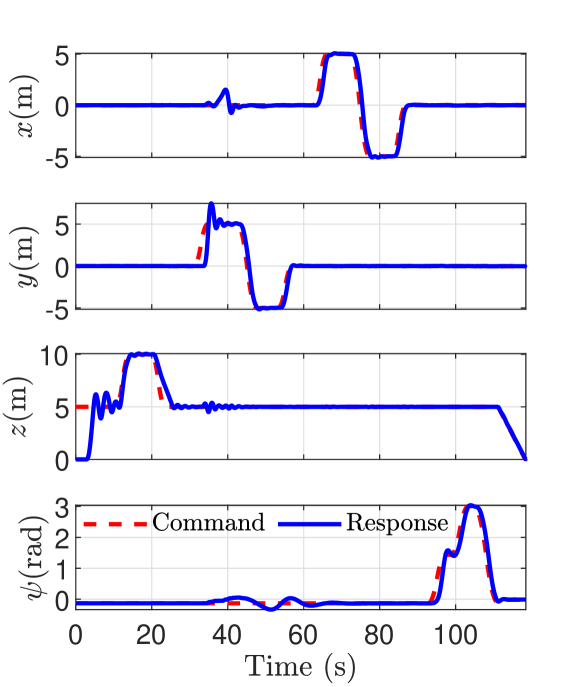
Figure 4: Simulation results. Response of the quadcopter in the learning trajectory in the jMAVSim simulator.

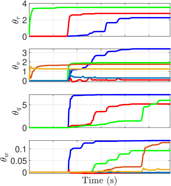
Figure 5: Simulation results. Autoilot gains adapted by the RCAC algorithm during the learning trajectory in the jMAVSim simulator.

Next, the quadcopter is commanded to follow a test trajectory, whose waypoints are generated using a second-order Hilbert curve, first with the default autopilot, and next with the autotuned autopilot. The default autopilot gains and the actuator constraints in PX4 are specified in the mc_pos_control_params.c, mc_att_control_params.c, and mc_rate_cont- rol_params.c files . Note that the results in this paper are based on PX4 version V1.11.3. Figure 6 shows the response of the quadcopter obtained with the autotuned autopilot and the default autopilot. Note that the autotuned autopilot outperforms the default autopilot in terms of position tracking error.

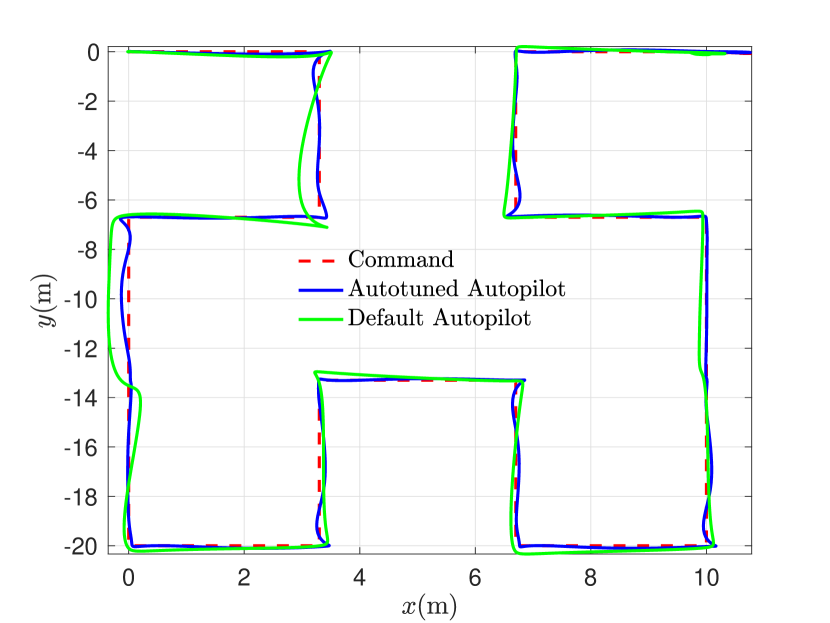
Figure 6: Simulation results. Response of the quadcopter in the test trajectory. Note that the autotuned autopilot uses the gains tuned during the learning trajectory.

In order to quantify and compare the performance of the autotuned autopilot with the default autopilot, a position-tracking cost variable $J$ defined by

$$J\stackrel{{\scriptstyle\triangle}}{{=}}\frac{1}{T}\sum_{i=0}^{N}z_{i}^{\rm T}z_{i},$$ (28)

where $z_{i}\in{\mathbb{R}}^{3}$ is the position error and $T$ is the total flight time in seconds, is computed for each test. Table III shows the cost default autopilot cost $J_{\rm D}$ and the autotuned autopilot cost $J_{\rm A}.$ Note that the autotuned autopilot is relatively 38 $\%$ better than the default autopilot in simulation.

TABLE III: Cost variable given by (28) for the autotuned and the default autopilots obtained in the test trajectory.

Test Type	$\begin{array}[]{c}\textbf{Default}\\ \textbf{Autopilot}\\ \textbf{Cost}\ \bm{(J_{\rm D})}\end{array}$	$\begin{array}[]{c}\textbf{Autotuned}\\ \textbf{Autopilot}\\ \textbf{Cost}\ \bm{(J_{\rm A})}\end{array}$	$\begin{array}[]{c}\textbf{Relative}\\ \textbf{Improvement}\\ \bm{(J_{\rm D}-J_{\rm A})/J_{\rm D}}\end{array}$
$\begin{array}[]{c}{\rm Simulation}\\ {\rm(jMAVSim)}\end{array}$	1.222	0.752	38.4 %
$\begin{array}[]{c}{\rm Flight\ Test}\\ {\rm(M}\text{-}{\rm Air)}\end{array}$	0.321	0.218	32.3 %

Next, the sensitivity of the autotuning process to changes in the physical parameters of the quadcopter is investigated. To do so, the mass of the quadcopter is scaled in the dynamic model simulated by jMAVSim. Specifically, the mass of the quadcopter is multiplied by $\alpha\in\{0.5,0.75,1,1.25,1.5\}.$ For each value of $\alpha,$ the autopilot gains are tuned using the autotuner. Note that the RCAC hyperparameters are not changed. The performance of the autotuned and the default autpilots is compared for each value of $\alpha$ by flying the test trajectory defined by the second-order Hilbert curve. Figure 7 shows the cost $J$ computed for the position controller in each flight flown with the autotuned and the default autopilot. Note that the autotuned autopilot is re-tuned for each value of $\alpha,$ whereas default autopilot is fixed for all values of $\alpha.$

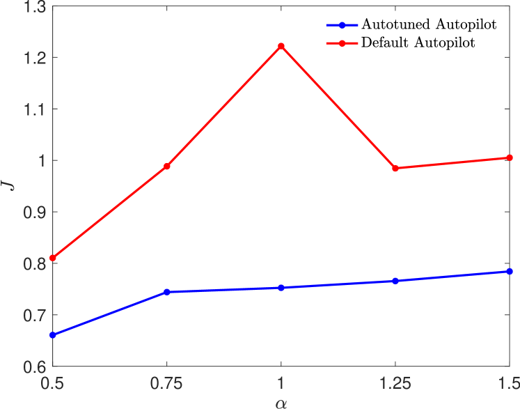
Figure 7: Simulation results. Position tracking cost in the test trajectory for the autotuned and the default autopilots obtained. Note that the mass of the quadcopter is multiplied by the scalar $\alpha$ in the jMAVSim simulation.

V-B Physical Flight Tests

Next, the autotuner is tested in physical flight tests conducted in the M-Air facility at the University of Michigan, Ann Arbor with the Holybro X500 quadcopter frame. The M-Air is equipped with a motion capture system that allows high-precision position and attitude measurements.

In the learning trajectory, $z_{\rm hov}=2$ m, $x_{\rm inc}=y_{\rm inc}=4$ m, and $z_{\rm inc}=1$ m. The guidance law generates the setpoints using $v_{\rm max}=3$ m/s, $a_{\rm max}=1.2$ m/${\rm s}^{2}$, $\dot{\psi}_{\rm max}=2$ rad/s, $\ddot{\psi}_{\rm max}=$ 0.5 rad/${\rm s}^{2}.$ Figure 8 shows the response of the quadcopter in the learning trajectory. Figure 9 shows the gains adapted by the RCAC algorithm for all four controllers.

Next, the quadcopter is commanded to follow a test trajectory with the autotuned autopilot and the default autopilot in the M-Air facility. The waypoints for the test trajectory are generated using a second-order Hilbert curve. Figure 10 shows the response of the quadcopter obtained with the autotuned autopilot and the default autopilot during the physical flight tests. Table III shows the position-tracking cost $J$ computed for the test trajectory flown during the physical flight tests. Note that the autotuned autopilot is relatively 32 $\%$ better than the default autopilot.

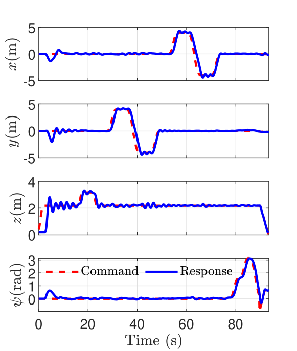
Figure 8: Flight test results. Response of the quadcopter in the learning trajectory at the M-Air facility.

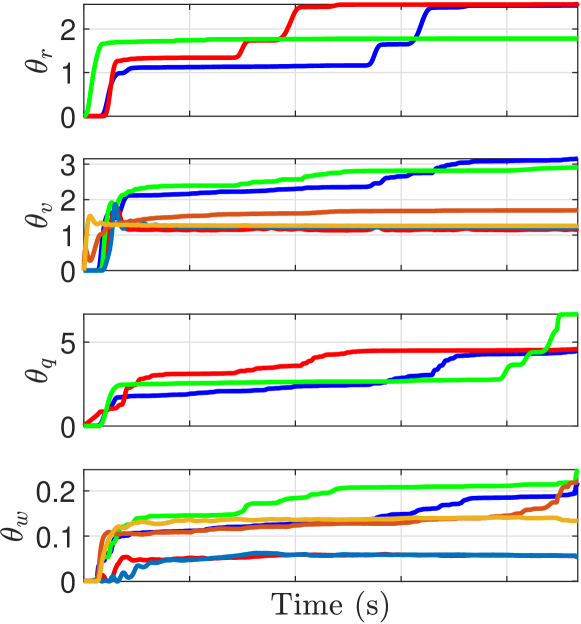
Figure 9: Flight test results. Autopilot gains adapted by the RCAC algorithm during the learning trajectory at the M-Air facility.

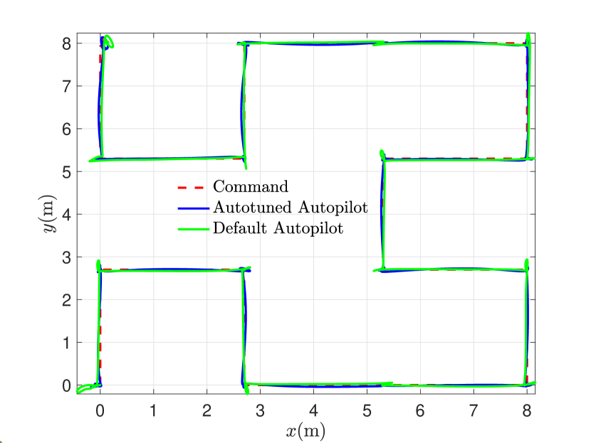
Figure 10: Flight test results. Response of the quadcopter in the test trajectory. Note that the autotuned autopilot uses the gains tuned during the learning trajectory.

VI Conclusions and Future Work

This paper presented an adaptive autotuner that can automatically tune a multicopter autopilot without using any modeling information about the multicopter. The adaptive autotuner, implemented in the PX4 flight stack, consists of adaptive PID controllers that are updated by the retrospective cost adaptive control algorithm by flying a single learning trajectory.

The adaptive autotuner was validated in a simulation environment, and its performance was compared against the default autopilot by scaling the mass of the quadcopter. The adaptive autotuner outperformed the default autotuner in all cases without any change in the hyperparameters of the adaptive algorithm. Next, using the same hyperparameters used for the simulation, the adaptive autotuner was used to tune the autopilot for the X500 Holybro quadcopter in the M-Air facility, where the adaptive autotuner outperformed the default autotuner in the test trajectory.

Future work will focus on using the adaptive autopilot to improve the performance of the default autopilot flying a multicopter with an unknown suspended payload and under various actuator failure conditions.

Appendix A

Let $r_{\rm c}\in{\mathbb{R}}^{3}$ denote the current position, $r_{\rm d}\in{\mathbb{R}}^{3}$ denote the desired position, and $d$ denote the distance between the current and the desired position, that is, $d\stackrel{{\scriptstyle\triangle}}{{=}}||r_{\rm d}-r_{\rm c}||_{2}.$ Let $a_{\rm max}>0$ and $v_{\rm max}>0.$ The desired trajectory consists of an acceleration phase, a cruise phase, and a deceleration phase along the straight line between $r_{\rm c}$ and $r_{\rm d}.$

Let the setpoints $r(t)\in{\mathbb{R}}^{3}$ be given by the guidance law

$$r(t)=r_{\rm c}+(r_{\rm d}-r_{\rm c})\frac{q(t)}{d},$$ (29)

where $q(t)$ is calculated as shown below. Using the fact that $r(0)=r_{\rm c}$ and $r(T_{\rm f})=r_{\rm d},$ where $T_{\rm f}$ is the total flight time, it follows that $q(0)=0$ and $q(T_{\rm f})=d.$ Note that $q(t)$ is the distance between $r(t)$ and $r_{\rm c}.$

Let $T_{1}$ denote the time to reach the speed $v_{\rm max}$ at maximum acceleration $a_{\rm max}.$ Thus, $T_{1}=\dfrac{v_{\rm max}}{a_{\rm max}}$ and $q(T_{1})=\dfrac{1}{2}a_{\rm max}T_{1}^{2}=\dfrac{1}{2}\dfrac{v_{\rm max}^{2}}{a_{\rm max}}.$

First, consider the case where $d\geq 2q(T_{1}).$ In this case, the quadcopter cruises at $v(t)=v_{\rm max}$ for $t\in[T_{1},T_{2}],$ where $t=T_{2}$ denotes the time at which deceleration phase starts, and is calculated as shown below. Note that

$$q(T_{2}) =\frac{1}{2}\frac{v_{\rm max}^{2}}{a_{\rm max}}+v_{\rm max}(T_{2}-T_{1}).$$ (30)

Since the quadcopter takes $T_{1}$ seconds to decelerate from $v_{\rm max}$ to $0$ speed at constant deceleration $a_{\rm max},$ the total flight time is $T_{\rm f}=T_{1}+T_{2}$ and

$$q(T_{3})=\frac{v_{\rm max}^{2}}{a_{\rm max}}+v_{\rm max}(T_{2}-T_{1})=d.$$ (31)

It follows from (31) that $T_{2}=\dfrac{d}{v_{\rm max}}$ and thus, the total flight time $T_{\rm f}=\dfrac{v_{\rm max}}{a_{\rm max}}+\dfrac{d}{v_{\rm max}}.$ The distance $q(t)$ is thus given by

$$q(t)=\begin{cases}\frac{1}{2}a_{\rm max}t^{2},&t\in[0,T_{1}),\\ \frac{1}{2}a_{\rm max}T_{1}^{2}+v_{\rm max}(t-T_{1}),&t\in[T_{1},T_{2}),\\ \frac{1}{2}a_{\rm max}T_{1}^{2}+v_{\rm max}(T_{2}-T_{1})\\ \quad+v_{\rm max}(t-T_{2})-\frac{1}{2}a_{\rm max}(t-T_{2})^{2},&t\in[T_{2},T_{\rm f}).\end{cases}$$ (32)

Next, consider the case where $d<2q(T_{1}).$ In this case, the quadcopter velocity does not reach $v_{\rm max}$, that is, there is no cruise phase. Let $\bar{T}_{1}$ denote the time instant at which maximum velocity $\bar{v}_{\rm max}$ is reached. Thus, $\bar{T}_{1}=\dfrac{\bar{v}_{\rm max}}{a_{\rm max}}$ and $q(\bar{T}_{1})=\dfrac{1}{2}\dfrac{\bar{v}_{\rm max}^{2}}{a_{\rm max}}.$ Assuming that the quadcopter decelerates at the same rate to rest, it follows that $q(\bar{T}_{1})=d/2,$ and thus $\bar{v}_{\rm max}=\sqrt{da_{\rm max}},$ $\bar{T}_{1}=\sqrt{\dfrac{d}{a_{\rm max}}},$and $T_{\rm f}=2\sqrt{\dfrac{d}{a_{\rm max}}}.$ The distance $q(t)$ is thus given by

$$q(t)=\begin{cases}\frac{1}{2}a_{\rm max}t^{2},&t\in[0,\bar{T}_{1}),\\ \frac{1}{2}a_{\rm max}\bar{T}_{1}^{2}+\bar{v}_{\rm max}(t-\bar{T}_{1})\\ \quad-\frac{1}{2}a_{\rm max}(t-\bar{T}_{1})^{2},&t\in[\bar{T}_{1},2T_{\rm f}).\end{cases}$$ (33)

References

- [1] C.-C. Chang, J.-L. Wang, C.-Y. Chang, M.-C. Liang, and M.-R. Lin, “Development of a multicopter-carried whole air sampling apparatus and its applications in environmental studies,” Chemosphere, vol. 144, pp. 484–492, 2016.
- [2] S. Anweiler and D. Piwowarski, “Multicopter platform prototype for environmental monitoring,” Journal of Cleaner Production, vol. 155, pp. 204–211, 2017.
- [3] V. H. Andaluz, E. López, D. Manobanda, F. Guamushig, F. Chicaiza, J. S. Sánchez, D. Rivas, F. Pérez, C. Sánchez, and V. Morales, “Nonlinear controller of quadcopters for agricultural monitoring,” in International Symposium on Visual Computing. Springer, 2015, pp. 476–487.
- [4] B. E. Schäfer, D. Picchi, T. Engelhardt, and D. Abel, “Multicopter unmanned aerial vehicle for automated inspection of wind turbines,” in 2016 24th Mediterranean Conference on Control and Automation (MED), 2016, pp. 244–249.
- [5] M. Stokkeland, K. Klausen, and T. A. Johansen, “Autonomous visual navigation of unmanned aerial vehicle for wind turbine inspection,” in 2015 International Conference on Unmanned Aircraft Systems (ICUAS), 2015, pp. 998–1007.
- [6] J. A. Paredes, J. González, C. Saito, and A. Flores, “Multispectral imaging system with uav integration capabilities for crop analysis,” in 2017 First IEEE International Symposium of Geoscience and Remote Sensing (GRSS-CHILE), 2017, pp. 1–4.
- [7] D. Lee, H. J. Kim, and S. Sastry, “Feedback linearization vs. adaptive sliding mode control for a quadrotor helicopter,” International Journal of control, Automation and systems, vol. 7, no. 3, pp. 419–428, 2009.
- [8] J. Farrell, M. Sharma, and M. Polycarpou, “Backstepping-based flight control with adaptive function approximation,” Journal of Guidance, Control, and Dynamics, vol. 28, no. 6, pp. 1089–1102, 2005.
- [9] P. Castillo, A. Dzul, and R. Lozano, “Real-time stabilization and tracking of a four-rotor mini rotorcraft,” IEEE Transactions on control systems technology, vol. 12, no. 4, pp. 510–516, 2004.
- [10] Z. Zuo and C. Wang, “Adaptive trajectory tracking control of output constrained multi-rotors systems,” IET Control Theory & Applications, vol. 8, no. 13, pp. 1163–1174, 2014.
- [11] Z. T. Dydek, A. M. Annaswamy, and E. Lavretsky, “Adaptive control of quadrotor uavs: A design trade study with flight evaluations,” IEEE Transactions on Control Systems Technology, vol. 21, no. 4, pp. 1400–1406, 2013.
- [12] Y. Abdolahi and A. Rezaeizadeh, “Black-box identification and iterative learning control for quadcopter,” in 2018 6th International Conference on Control Engineering & Information Technology (CEIT). IEEE, 2018, pp. 1–5.
- [13] A. R. Dooraki and D.-J. Lee, “Reinforcement learning based flight controller capable of controlling a quadcopter with four, three and two working motors,” in 2020 20th International Conference on Control, Automation and Systems (ICCAS). IEEE, 2020, pp. 161–166.
- [14] K. M. Thu and G. A. Igorevich, “Modeling and design optimization for quadcopter control system using L1 adaptive control,” in 2016 IEEE 7th Annual Information Technology, Electronics and Mobile Communication Conference (IEMCON). IEEE, 2016, pp. 1–5.
- [15] V. P. Tran, F. Santoso, M. A. Garratt, and I. R. Petersen, “Fuzzy self-tuning of strictly negative-imaginary controllers for trajectory tracking of a quadcopter unmanned aerial vehicle,” IEEE Transactions on Industrial Electronics, vol. 68, no. 6, pp. 5036–5045, 2020.
- [16] P. k. Muthusamy, M. Garratt, H. R. Pota, and R. Muthusamy, “Real-time adaptive intelligent control system for quadcopter UAV with payload uncertainties,” IEEE Transactions on Industrial Electronics, 2021.
- [17] E. A. Niit and W. J. Smit, “Integration of model reference adaptive control (MRAC) with PX4 firmware for quadcopters,” in 2017 24th International Conference on Mechatronics and Machine Vision in Practice (M2VIP). IEEE, 2017, pp. 1–6.
- [18] V. Hoang, M. D. Phung, and Q. P. Ha, “Adaptive twisting sliding mode control for quadrotor unmanned aerial vehicles,” in 2017 11th Asian Control Conference (ASCC). IEEE, 2017, pp. 671–676.
- [19] B. G. Czakó and K. Kósi, “Novel method for quadcopter controlling using nonlinear adaptive control based on robust fixed point transformation phenomena,” in 2017 IEEE 15th International Symposium on Applied Machine Intelligence and Informatics (SAMI). IEEE, 2017, pp. 000 289–000 294.
- [20] E. Yazid, M. Garrat, and F. Santoso, “Optimal PD tracking control of a quadcopter drone using adaptive PSO algorithm,” in 2018 International Conference on Computer, Control, Informatics and its Applications (IC3INA). IEEE, 2018, pp. 146–151.
- [21] A. K. Bhatia, J. Jiang, Z. Zhen, N. Ahmed, and A. Rohra, “Projection modification based robust adaptive backstepping control for multipurpose quadcopter UAV,” IEEE Access, vol. 7, pp. 154 121–154 130, 2019.
- [22] A. Kourani, K. Kassem, and N. Daher, “Coping with quadcopter payload variation via adaptive robust control,” in 2018 IEEE International Multidisciplinary Conference on Engineering Technology (IMCET). IEEE, 2018, pp. 1–6.
- [23] M. Navabi and S. Soleymanpour, “Immersion and invariance based adaptive control of aerial robot in presence of inertia uncertainty,” in 2017 IEEE 4th International Conference on Knowledge-Based Engineering and Innovation (KBEI). IEEE, 2017, pp. 0959–0964.
- [24] A. Tabata, Y. Satoh, H. Nakamura, and K. Kato, “Adaptive fault tolerant control of quadcopter by using minimum projection method,” in IECON 2018-44th Annual Conference of the IEEE Industrial Electronics Society. IEEE, 2018, pp. 2201–2206.
- [25] X. Hu and J. Liu, “Research on uav balance control based on expert-fuzzy adaptive PID,” in 2020 IEEE International Conference on Advances in Electrical Engineering and Computer Applications (AEECA). IEEE, 2020, pp. 787–789.
- [26] L. Zhang, F. Yang, W.-y. Zhou, J. Huang, and X. Su, “Pitch angle control of UAV based on L1 adaptive control law,” in 2020 35th Youth Academic Annual Conference of Chinese Association of Automation (YAC). IEEE, 2020, pp. 68–72.
- [27] W. Li, W. Zhang, J. Shi, X. Qu, Y. Fu, J. Che, and H. Zhou, “Lateral control reconfiguration of tailless flying-wing UAV based on L1 adaptive control method,” in 2018 IEEE CSAA Guidance, Navigation and Control Conference (CGNCC). IEEE, 2018, pp. 1–7.
- [28] W. Yu, D. Lin, and T. Song, “Adaptive control for UAV close formation flight against disturbances,” in 2018 3rd International Conference on Robotics and Automation Engineering (ICRAE). IEEE, 2018, pp. 196–201.
- [29] H. Gui, R. Sun, and J. Chen, “Adaptive parameter estimation and velocity control of uav systems,” in 2018 37th Chinese Control Conference (CCC). IEEE, 2018, pp. 9866–9871.
- [30] L. Meier, D. Honegger, and M. Pollefeys, “Px4: A node-based multithreaded open source robotics framework for deeply embedded platforms,” in 2015 IEEE international conference on robotics and automation (ICRA), 2015, pp. 6235–6240.
- [31] ArduPilot Dev Team, “Ardupilot,” https://ardupilot.org/ardupilot/.
- [32] M. Kamaldar, S. A. U. Islam, S. Sanjeevini, A. Goel, J. B. Hoagg, and D. S. Bernstein, “Adaptive digital PID control of first-order-lag-plus-dead-time dynamics with sensor, actuator, and feedback nonlinearities,” Advanced Control for Applications, vol. 1, no. 1, p. e20, 2019.
- [33] A. Goel, J. A. Paredes, H. Dadhaniya, S. A. Ul Islam, A. M. Salim, S. Ravela, and D. Bernstein, “Experimental implementation of an adaptive digital autopilot,” in 2021 American Control Conference (ACC), 2021, pp. 3737–3742.
- [34] N. A. Chaturvedi, A. K. Sanyal, and N. H. McClamroch, “Rigid-Body Attitude Control,” IEEE Control Systems Magazine, vol. 31, no. 3, pp. 30–51, 2011.
- [35] Y. Rahman, A. Xie, and D. S. Bernstein, “Retrospective Cost Adaptive Control: Pole Placement, Frequency Response, and Connections with LQG Control,” IEEE Control System Magazine, vol. 37, pp. 28–69, 10 2017.
- [36] A. Goel, S. A. U. Islam, and D. S. Bernstein, “Adaptive Control of MIMO Systems Using Sparsely Parameterized Controllers,” in 2020 American Control Conference (ACC), 7 2020, pp. 5340–5345.
- [37] S. A. U. Islam and D. S. Bernstein, “Recursive Least Squares for Real-Time Implementation,” IEEE Control Systems Magazine, vol. 39, no. 3, pp. 82–85, 6 2019.