Efficient Non-linear Calculators

Abstract

A novel algorithm for producing smooth nonlinearities on digital hardware is presented. The non-linearities are inherently quadratic and have both symmetrical and asymmetrical variants. The integer (and fixed point) implementation is highly amenable for use with digital gates on an ASIC or FPGA. The implementations are multiplier-less. Scaling of the non-linear output, as required in an LSTM cell, is integrated into the implementation. This too does not require a multiplier.

The non-linearities are useful as activation functions in a variety of ANN architectures. The floating point mappings have been compared with other non-linearities and have been benchmarked. Results show that these functions should be considered in the ANN design phase.

The hardware resource usage of the implementations have been thoroughly investigated. Our results make a strong case for implementations in edge applications. This document summarizes the findings and serves to give a quick overview of the outcomes of our research.

I Motivation

The General Matrix Multiplication (GEMM) typically computes $\bar{n}=\bar{w}\times\bar{p}+\bar{b}$. In deep learning, $w$ are weights, $p$ is an input, $b$ is a bias term and $n$ is the netsum. The GEMM is the most computationally heavy workload in deep learning. The computation of the GEMM has evolved to reduce the computational complexity in terms of both memory and latency. Several optimizations and parallelization techniques have been proposed in the literature. Without a fast and resource efficient GEMM facility, Artificial Neural Network (ANN) algorithms would be dominated by the sheer volume of multiplication (MUL) instructions. With the availability of fast and resource efficient GEMM operations, the computationally complex activation functions (functions with exponent, logarithm, trigonometric, and floating-point division) become more significant and can dominate the computational load [Wuraola et al., 2021]. Therefore, a fast and resource efficient activation function is essential to maintain the throughput of the GEMM.

II The Algorithm

In principle, the algorithm for generating a non-linear mapping, $f(n)$, can be written as ${f(n)=\mbox{mean}((n+r)-r)}$ where $n$ is a netsum i.e. the output of a GEMM and $r$ is a random number. The algorithm hinges on saturation of the addition operation, the saturation levels and the range of the random values. Hence, an appropriate representation of the algorithm is given by -

$$f(n)=\frac{1}{N}\sum_{k=1}^{N}f_{sat}\left(f_{sat}(n+U(k),C)-U(k),M\right)$$ (1)

Here,

• $n$ is a signed integer encoded with 2’s complement

• $R$ is the bit width of the binary word used to represent $n$. The 2’s complement representation implies that ${2^{R-1}\leq n<2^{R-1}}$. The output, $f(n)$ is also 2’s complement encoded with a width of $R$ bits.

• The addition and subtraction operations are saturating, i.e.,

  $$f_{sat}(x,Y)=\left\{\begin{array}[]{ll}-Y&:x\leq-Y\\ x&:-Y<x<Y\\ Y&:x\geq Y\\ \end{array}\right.$$ (2)

• $M=2^{R-1}$ and $0\leq C<2^{R-2}$.

• $U(k)$ is a predefined non-repeating sequence of integers,

• $N$ is the length of $U(k)$.

The current implementation of this algorithm produces an integer non-linear mapping from an integer input.

III Concepts

The TanSig/LogSig mappings will used to explain the concept. The technique is visualized in Fig. 1 while a block diagramatic view is shown in Fig. 2.

First, the input i.e. the netsum and a random signal (uniform distribution with a range of $\pm 1.0$) are added. The random signal is oversampled and hence the input is added to several random values. The adder is saturating (hard-limited) and hence all sums more than the defined limits are clipped. The same random signal is then subtracted from the sum. The subtraction attempts to recover the original input. If the input was small in magnitude then the addition with the random signal will not eventuate in clipping (in any of the oversampled sums) and hence the original input is recovered after the subtraction. Fig. 1 shows this scenario around $(0,0)$. However, if the input is large in magnitude then, for a small subset, the addition of the random values will lead to clipping and then the following subtraction will not restore the original signal. The filter smooths the restored outputs but since a subset has reduced magnitude the filtered outputs will also be reduced in magnitude. The resulting transfer characteristic is non-linear. Fig. 1 shows this around $\approx(1,1)$. If the distribution of the random signal has a very small variance then the non-linearity will be narrower i.e. it will not manifest till the signal is very close to $(1,1)$. However, if the variance is large then the non-linearity is manifest much before $(1,1)$ i.e. closer to $(0,0)$. Hence the variance can be used to shape the non-linearity.

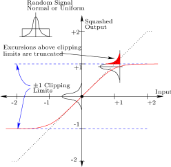
Figure 1: Pictorial Description of Transfer Characteristics of the Proposed Method

Figure 2: Block Schematic of Proposed Square Law Squashing Function

Fig. 2 has been simulated in Matlab. A uniform distribution with a range of $\pm 1.0$ was used. The adder has its hard-limit set at $\pm 1.0$ while the subtracter is at $\pm 2.0$. The data at $f_{1}(x)$ was fitted to an approximate TanSig function defined in Eq. 3. A particular Matlab simulation results in $a=-1.81$ and $b=0.18$ (c.f. $a=-2.0$ and $b=0$ for TanSig) and exhibiting RMS error of 0.023. Thus $f_{1}(x)\approx f_{A}(x)$.

$$f_{A}(x)=\frac{2}{1+e^{ax+bx^{3}}}-1$$ (3)

Fig. 3 plots the Matlab simulation. The traces with the jitter are the outputs of the simulated squashing function while the solid trace is a plot of Eq. 3 with the fitted parameters.

If $f_{1}(x)$ is scaled and shifted by +0.5, an approximate LogSig is produced. This has also been simulated and presented in Fig. 3.

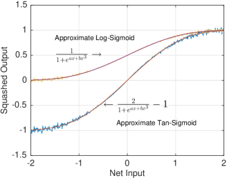
Figure 3: Simulated Squashing Functions Showing Approximate TanSig and LogSig Behavior

In reality, a random source is not required required and can, in fact, be implemented using only a binary counter. Thus, in eq 1, $U(k)$ is produced by a binary counter. Both symmetrical and asymmetrical mappings can be produced.

IV Related work

In literature, various approaches have been proposed for implementing efficient hardware transcendental activation functions.These methods fall into 3 broad categories: LUT, piecewise approximation, and hybrid methods. LUT is used to store the values of the activation functions as used in neurons. LUTs require pre-calculation of the activation functions mapping before being loaded into memory. As described in [Yang et al., 2018], the activation function values are divided into equal subranges, each subrange is approximated by a value stored in the FPGA read only memory. LUT method has been shown to be generally resource and memory intensive for higher resolution and precision [Tan et al., 2007]. The structure of a LUT is not amenable to direct expansion when there is a need for factors such as a change in resolution, activation function, and so on.

Piecewise approximation of transcendental activation functions are divided into different types which include piecewise linear [Amin et al., 1997, Larkin et al., 2006], piecewise nonlinear [Pushpa and Manimala, 2014], and others [Tiwari and Khare, 2015, Yang et al., 2018]. Piecewise linear approximation uses the basic form of $f(x)=ax+b$ (where a is the function slope, b is the intercept) to construct exponential-based activation functions. The authors in [Amin et al., 1997, Larkin et al., 2006] use 12 breakpoints with their solution requiring multiple IF ELSE statements, LUT to store coefficients, multiplier and adder. The use of approximation formula as described in [Gomar et al., 2016] is based on using formula to approximate the exponential function present in exponential-based activation function as shown $e^{x}\approx Ex(x)\approx 2^{1.44x}$. Based on this formulation, sigmoid activation function can be calculated as $f(x)\approx\frac{1}{1+2^{-1.44x}}$. Computationally, this method requires four clock cycles to approximate the sigmoid function. The computation of sigmoid function will require an add, a subtract, a division, a multiplier and an exponent. The disadvantage of this method is high computational resource utilisation and high latency. Taylor series expansion is the most common example of piecewise nonlinear approximation for exponential-based activation functions. An advantage of Taylor series expansion is that it can be used to approximate an activation function to any precision. However, this comes at a cost of resource utilisation (several multipliers) and high latency (several clock cycles). The Taylor series expansion is of the form $f(x)=\sum_{\infty}^{n=0}\frac{f^{(n)}(x_{0})}{n!}(x-x_{0})^{n}$. Taylor series approximation method can be combined with LUT based method and this is normally referred to as optimised/hybrid LUT. As described in [Yang et al., 2018], LUT is combined with piecewise nonlinear Taylor series expansion. The Taylor series expansion is applied to the activation function. The authors used a fifth-order expansion for Tanh ($f(x)=x+\frac{x^{3}}{3}+\frac{2x^{5}}{15}$), when $\frac{x^{3}}{3}+\frac{2x^{5}}{15}<=0.02$, $f(x)\approx x$. Solving the inequality results in $x>=0.39$ and Tanh$(2.90)\approx 1$. Therefore, only the values input $x$ in the range $0.39-2.90$ need to be stored in an LUT. Furthermore, authors in [Larkin et al., 2006] makes use of minimax polynomial approximation. A minimax polynomial exists for every approximation method and can minimise the maximum error by evenly distributing the errors across the entire approximation range as opposed to the use of Taylor series expansion. The authors proposed the use of lower order polynomial by sub-dividing the input domain into smaller intervals using the Remez exchange algorithm. The Remez exchange algorithm is used to find approximate coefficients to generate minimax polynomials on discrete intervals [Larkin et al., 2006]. This method requires the use of LUT, multiplier and adder.

In most cases, piecewise approximation requires one or more multipliers [Larkin et al., 2006]. As described in [Courbariaux et al., 2014, Hubara et al., 2016] multipliers are resource hungry and power-hungry devices on hardware. Other types of piecewise approximation have been shown not to require any multiplier but rather only comparators, multiplexers, shift operators, storage of several coefficients. Hard Tanh and sigmoid fall into these categories too. For a small degradation in performance accuracy for some problem space, hard and shift operators based piecewise approximation activation functions will suffice.

FPGA implementation of LSTM has been explored in literature [Cao et al., 2019, Ferreira and Fonseca, 2016, Han et al., 2017, Rybalkin et al., 2018]. LSTM’s computational intensity has led to various ways of efficient implementation of LSTM. Weight pruning and compression are techniques that lower memory requirements and reduce complexity [Han et al., 2017]. Other complexity reduction methods are data representation and multiplier reduction through sparse LSTM. In literature, data representation in LSTM model go from 32 bits to binary [Rybalkin et al., 2018]. Commonly the activations and weights are represented with 8-bits or 16-bits [Cao et al., 2019, Ferreira and Fonseca, 2016, Han et al., 2017]. The use of the approximate multiplier [Azari and Vrudhula, 2019, Sim and Lee, 2017] is on the increase in hardware neural networks. The approximate multiplier developed in [Sim and Lee, 2017] and extended in [Azari and Vrudhula, 2019] includes hierarchical controllers that synchronize the variable cycle multiply operations with other single-cycle units. The principle is based on stochastic computing which allows for low cost and power but with increased fluctuation error and long latency. Its main component is a Finite State Machine (FSM) with $2^{n}$ states that generates a specific bit-stream. The proposed design requires a variable number of clock cycles, which depend on the magnitude of the operands. The advantages of the designs in [Azari and Vrudhula, 2019, Sim and Lee, 2017] are its low logic complexity, reduced power consumption and high error tolerance but with an increase in resource utilisation.Two popular works in literature have developed LSTM FPGA inference Engine namely C-LSTM [Wang et al., 2018] and Efficient Speech Recognition Engine (ESE) [Han et al., 2017]. The authors [Han et al., 2017], build an ESE engine with sparse LSTM on FPGA. In the model, 16 multipliers were instantiated for element-wise multiplications per channel (total channel is 32).

V Implementation

The algorithm (Equation 1) can be adapted to generate both symmetric and asymmetric mappings.

V-A Symmetric Activation Function - Square Law Nonlinearity (SQNL)

Given a word size $R$, the symmetric activation function generator will use the following parameters:

• $C=2^{R-2}$ and $M=2^{R-1}$

• $U(k)=\{-U_{MAX},\cdots,U_{MAX}\}$ with $U_{MAX}=C=2^{R-2}$. The length of $U(k)$ is a design decision.

With these parameters, the mapping can, analytically, be shown to be -

$$f(n)=\left\{\begin{array}[]{ll}-\frac{M}{2}&:n<-M\\ n+\frac{n^{2}}{2M}&:-M\leq n<0\\ n-\frac{n^{2}}{2M}&:0\leq n\leq M\\ \frac{M}{2}&:n>M\end{array}\right.$$ (4)

Figure 4 shows the implementation schematic and can be easily translated into HDL. The symmetric mapping requires Counter1 (alpha and Counter2 are required for the asymmetric generator). The resolution of the GEMM operation will typically be of a higher resolution and hence may need to be resized before obtaining the non-linear mapping.

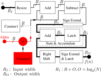
Figure 4: Schematics of Symmetric and Asymmetric Activation Function Generator

Figure 8 shows the SQNL mapping with $R=8$ and $N=8$. The SQNL is morphologically similar to the TanSig function. Although it is not symmetrical, the LogSQNL is also shown. It can be derived, in hardware, from the SQNL with almost zero hardware overhead because the divide by 2 (Div2) and offset reduce to ’shift’ operations.

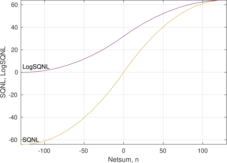
Figure 5: Symmetrical mapping with $R=8$ and $N=8$

With $R=8$ i.e. $-128\leq n<127$, the output range is $-64\leq f(n)\leq 63$ and $2\leq N\leq 2^{R-1}$. The interative nature of Equation 1 implies a smaller value length of $U(k)$ is attractive. With $N=2^{R-1}$ the mapping is perfectly smooth and perfectly . With $N<2^{R-1}$ the mapping becomes piecewise linear. In Figure 5 with $N=8$ the mapping shows 16 linear segments that are evenly distributed across $-64\leq f(n)\leq 63$. The deviation of the piecewise linear mappings from Equation 1 are developed.

Figure 6 plots the deviations with $N=4$ and $N=8$. The deviation is at maximum when $n$ is equal to any of the values of $U(k)$ and zero midway between any two consecutive $U(k)$. As expected, the profile shows a reduction in deviation with an increase in $N$.

Figure 7 shows the distribution of the deviations with $N=4$ and $N=8$. It shows that the deviations, for both, are at most $\pm 1$ bit away from the ideal mapping. With $N=8$ the histogram shows that the deviations are within $\pm 0.25$. Theoretically, there will be a zero-bit error if $N=8$ when $R=8$. However, if $N$ is reduced to 4, more than 70% of the range will still exhibit zero-bit errors.

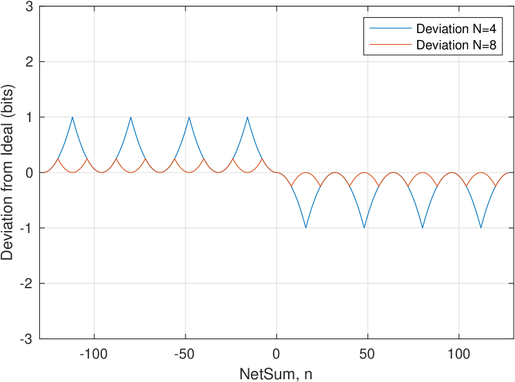
Figure 6: Deviation from ideal for $R=8$ at $N=$ 4 and 8

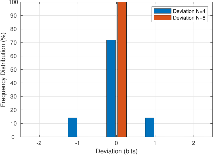
Figure 7: Histograms of the deviation from ideal for $R=8$ at $N=$ 4 and 8

V-B Asymmetrical Activation Function

Given a word size $R$, the asymmetric activation function generator will use the following parameters:

• $U(k)=\{-2U_{MAX},\cdots,0\}+\alpha$, where $0\leq\alpha\leq\frac{M}{2}$

• Adder saturates at $C=\{-U_{MAX},M\}$, where
  $U_{MAX}=2^{R-2}$ and $M=2^{R-1}$, i.e., only the lower saturation boundary is required

With these parameters, the mapping can, analytically, be shown to be -

$$f(n)=\left\{\begin{array}[]{ll}-\alpha&:n<-\frac{M}{2}-\alpha\\ \frac{(\frac{M}{2}+n+\alpha)^{2}}{2M}-\alpha&:-\frac{M}{2}-\alpha\leq n\leq\frac{M}{2}-\alpha\\ n&:n>\frac{M}{2}-\alpha\\ \end{array}\right.$$ (5)

A hardware implementation would require the ’alpha’ and ’Counter2’ elements in Figure 4. The asymmetrical mappings are shown in Figure 8. With $\alpha=0$, the mapping is similar to the SoftPlus function while with $\alpha>0$ is similar to the ELU function. It should be highlighted that the mappings are not exponential and inherently quadratic.

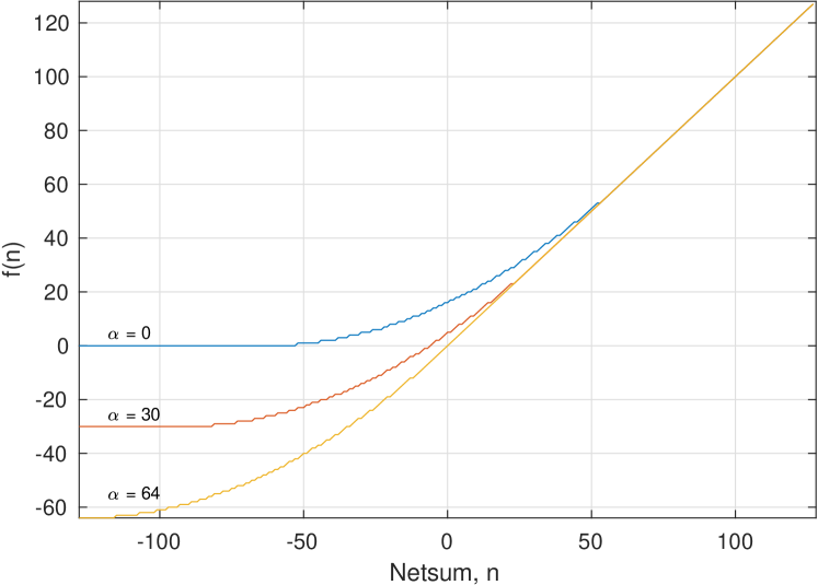
Figure 8: Asymmetrical mappings with $R=8$ and $N=8$

V-C The Gated Activation (Scaled SQNL)

LTSM cells, Figure 9 require a bitwise scaling of a TangSig activation function with the output of an LogSig activation function. Each cell requires 3 multiplications.

In the earlier sections we have shown an ability to make, in hardware, activation functions that are morphologically similar to both the TanSig and the LogSig. A modification to the SQNL schematic can integrate the scaling operation with a relatively small overhead in hardware resources. Specifically, the adder block is modified such that its saturation level is set by the required scaling. This is shown in Figure 10. This, in-effect, achieves a scaling without requiring a physical multiplier. The mapping, Equation 6 has been derived.

Figure 9: A Conventional LSTM Cell

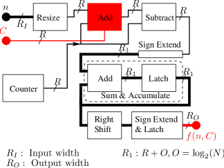
Figure 10: Schematic of the digital implementation of gated activation method.

$$f(n,C)=\left\{\begin{array}[]{ll}-C&:n<-(U_{MAX}+C)\\ n+\frac{(-\bigtriangleup+n)^{2}}{4U_{MAX}}&:-(U_{MAX}+C)\leq n<-\bigtriangleup\\ n\frac{C}{U_{MAX}}&:-\bigtriangleup\leq n\leq\bigtriangleup\\ n-\frac{(\bigtriangleup+n)^{2}}{4U_{MAX}}&:\bigtriangleup<n\leq(U_{MAX}+C)\\ C&:n>(U_{MAX}+C)\end{array}\right.$$ (6)

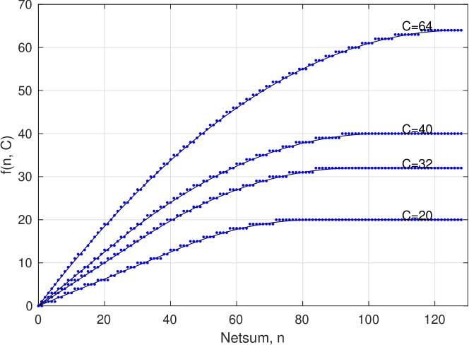
Figure 11: Gated Activations for $R=8$, $N=4$

At the limit, $C=2^{R-2}=U_{MAX}$ and if $G(n)=f(n,2^{R-2})$ then Equation 6 gives ${f(n,C)\approx m\times G(n)}$ where $m=C/U_{MAX}$. The range of the LogSQNL is $[0,2^{R-2}]$ and hence it can be connected to the $C$ port. This implements a scaling as required in the bitwise multiplication in LSTMs. The mappings of $f(n,C)$, with $R=8$ and $N=8$, for different values of $n$ and $C$ are shown in Figure 11. This figure also overlays Equation 6 with a solid black trace.

The algorithm as modelled by Equation 6 exhibits a small error from the ideal ${m\times G(n)}$. The plot with $C=64$ corresponds to ${G(n)=f(n,64)}$. With $C=40$, ${f(n,40)\approx\frac{40}{64}G(n)}$. Specifically at $n=40$, ${G(40)=33.75}$, ${f(40,40)=24}$ but ${\frac{40}{64}\times 33.75=21.09}$ and hence, the gated activation exhibits an error of $-2.91$. The error can be determined by Equation 7.

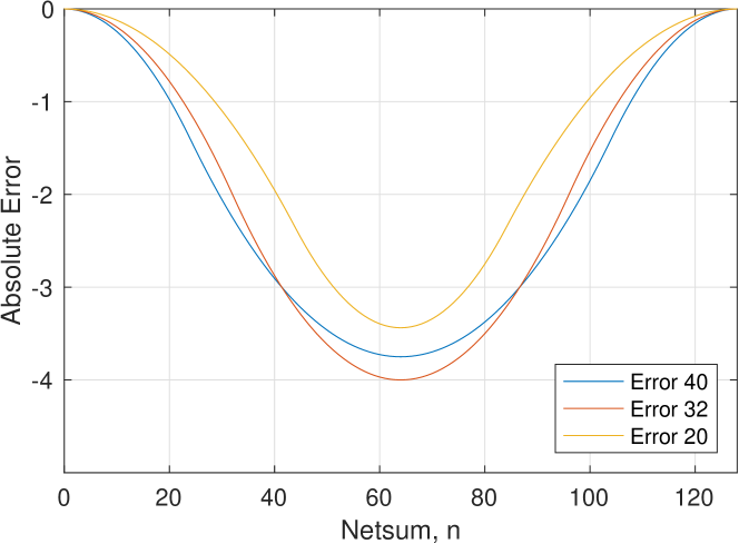
Figure 12: Error between $m\times G(n)$ and $f(n,C)$

$$E(n,C)=\frac{C}{U_{MAX}}\times G(n)-\left(n+\frac{-(\bigtriangleup+n)^{2}}{4U_{MAX}})\right)$$ (7)

Thus, an LSTM Cell can be implemented using the SQNL by replacing the TanSig and LogSig activation functions with the SQNL eqivalents. Additionally, the gated activation effectively eliminates two of the three multipliers as well. An LSTM Cell using the SQNL is shown in Figure 13. In work, we also propose a lower cost multiplier (QSU) that capitalizes on the reduced bit-widths. This eliminates all multipliers in the cell.

Figure 13: An LSTM Cell using SQNL

Remarks

1. The input range of the SQNL activation function (Equation 4) is between $[-\infty,+\infty]$. The output is continuous and bounded. The SQNL family of functions are easily differentiable and satisfies the requirements of the universal approximation theorem [Hornik et al., 1989, Leshno et al., 1993].

2. The derivatives are well-behaved and computationally attractive.

3. From a computational perspective, the quadratic is the simplist non-linearity. If a non-linear activation is required, the SQNL function is the most computationally efficient non-linearity for both inferencing and learning on ASICs, FPGAs, or CPUs.

4. The benefits of an hardware implementation of SQNL can be realised with or without the availability of hardware multipliers.

VI Resource Utilization

The SQNL algorithm can be implemented using standard building blocks. If hardware multipliers are available, the closed-form quadratic equations can be implemented instead.

The real-estate on silicon is dependent on the target chip technology. The metrics shown here has based on a an Intel Cyclone V compiled using Quartus Prime ver 18.1. On FPGAs, the basic building block is vendor dependent and hence we have also attempted to offer a vendor independent metric. To do this, we assume that the basic building block is a NAND gate. With this assumption, we estimate the gate usage for the relevant building blocks and shown in Table I. The SQNL blocks can then be quantified using these building blocks. These indicative metrics will be used in all subsequent comparisons.

TABLE I: Indicative Gate Usage

Digital Block	Cell/bit	Gates/bit	Total Gate
Single register	-	-	4
1bit full adder	-	-	9
8bit adder	-	-	72
9bit adder	-	-	81
8bit 2’s Complement	-	-	80
9bit 2’s Complement	-	-	90
2 to 1 mux (1bit)	-	3	3
LUT 8 bits (1-sided)	127	381	2667
LUT 12 bits (1-sided)	2047	6141	67551
LUT 8 bits (2-sided)	255	765	6120
LUT 12 bits (2-sided)	4095	12285	147420
Booth 8 bits	-	-	754
Booth 12 bits	-	-	1124

The comparison of the SQNL was undertaken with competing techniques: LUT, PWL and multipliers. To determine the gate usage of a multiplier, we use a custom implementation of a radix 4 multiplier and coded in HDL. The gate usage is also listed in Table I.

TABLE II: Resource utilization of symmetric and asymmetric functions implementation using a custom Booths Radix-4 multiplier (mult), multi-clock (counter, $N=8$), and LUT solution. As displayed the counter based method for the two function types consistently outperform the multiplier solution on both ASIC and FPGA platforms. At a lower resolution, the LUT performs slightly better than the counter solution on FPGA but worse on ASIC when compared with the counter solution. The LUT on the other hand is only better for lower resolution and can not accommodate applications where higher resolution is required. The counter solution scales well across different resolutions.

		Symmetric			Asymmetric
		SQNL			SQLU ($\alpha=2^{R-2}$)			SQ_Softplus ($\alpha=0$)
R	Methods	Gates	ALM	FF	Gates	ALM	FF	Gates	ALM	FF
8	Mult	963	120	63	987	124	63	826	100	54
	LUT	2779	17	8	2779	17	8	2747	19	8
	Counter	388	34	24	460	31	22	460	29	24
12	Mult	1400	180	93	1473	187	93	1232	153	80
	LUT	67719	234	12	67719	234	12	67671	125	12
	Counter	556	46	31	664	41	31	664	39	30

A detailed analysis of the implementation is discussed in a manuscript that is under second review. Below we summarize our comparisons of the SQNL with competing techniques.

• Counter - At low/mid resolutions the counter based solution gives the maximum density of activation functions. The counter-based solution permits the encapsulation of symmetric and asymmetric functions into a single entity. Thus activation functions can be dynamically adapted during training and inferencing. Our experiments on various models show that the absolute error due to $N\leq 8$ has no impact on model performance. However if $R>16\mbox{ and }N>16$, the multiplier may be more efficient but if $N\leq 8$ the counter based method is much more attractive.

• Multiplier - A multiplier solution would be attractive if free multipliers are available and if high/full precision is essential. Furthermore, since our square-law based functions are not an approximation, the direct solution will not introduce any approximation errors when compared to the PWL methods found in the literature. The conditionals in Equation 4 and 5 can be implemented using combinatorial logic. This will lead to addition timing overhead from propagation delay but will not require additional clocks.

• LUT - A LUT based function underperforms compared with a counter-based solution. At higher resolutions, the LUT is not a practical option due to excessive gate usage. At lower resolutions ($R<8$), a LUT may outperform a counter-based solution on an FPGA but this is device-dependent.

The resource usage implications for an LSTM cell have also been detailed. In summary,

• Piecewise Linear Approximation - Each of the 5 activation functions will require 5 multipliers and an additional 3 multipliers for bitwise operations. Assuming 3 multiplications per DSP would imply a minimum of 3 DSPs but the fitter reports usage of 7 DSPs. Increasing the resolution to 16 bits should result in 4 DSP blocks but again the fitter reports only 7 DSPs. It is possible that the data flow necessitates the allocation of multipliers in individual DSPs.

• Lookup Table - With this method, the table values are stored in the LUT’s within the ALMs. The three bitwise multipliers would ideally require a single DSP but the fitter reports 2 DSPs. As expected, the 16-bit cell shows a big increase in ALM usage to store the table also requires 2 DSPs. As with the PWL method, the data flow necessitates the allocation of multipliers in individual DSPs.

• Hard Tanh and Hard Sigmoid - The hard activations are the simplest to implement and the bulk of the resource usage will be used to effect the saturation logic at the breakpoints. As with the Lookup Table method, bitwise multipliers require 2 DSPs for both 8 and 16-bit resolutions.

TABLE III: Resource utilization of LSTM cell

Method	8 bits			16 bits
	ALM	FF	DSP	ALM	FF	DSP
Piecewise Activation [Wang et al., 2018]	81	-	7	107	-	7
LUT [Han et al., 2017]	96	16	2	6,568	32	2
Hard Activation	20	-	2	53	-	2
Gated Activation (Proposed)	52	55	-	150	175	-

VII SQNL Family for Simulations

The mappings developed for hardware implementation may have a restrictive use in simulation frameworks. These quadratic mappings can be translated to suit CPUs implementations.

VII-A SQNL

Equivalent to the TanSig (TanH) mapping -

$$f(n)=\left\{\begin{array}[]{ll}1&:n>2.0\\ n-\frac{n^{2}}{4}&:0\leq n\leq 2.0\\ n+\frac{n^{2}}{4}&:-2.0\leq n<0\\ -1&:n<-2.0\end{array}\right.$$

VII-B SQ_LogSig

Equivalent to the Sigmoid mapping -

$$f(n)=\frac{f_{SQNL}}{2}+0.5$$

VII-C SQLU

Equivalent to the ELU mapping -

$$f(n)=\left\{\begin{array}[]{ll}n&:n>0\\ n+\frac{n^{2}}{4}&:-2.0\leq n\leq 0\\ -1&:n<-2.0\end{array}\right.$$

VII-D SQ_SOFTMAX

Equivalent to the Softmax mapping -

$$f(n)=\left\{\begin{array}[]{ll}n&:n>0.5\\ \frac{(n+0.5)^{2}}{2}&:-0.5\leq n\leq 0.5\\ 0&:n<-0.5\end{array}\right.$$

VII-E SQ_SQISH

Equivalent to the SQISH mapping -

$$f(n)=\left\{\begin{array}[]{ll}n+\frac{n^{2}}{32}&:n>0\\ n+\frac{n^{2}}{2}&:-2.0\leq n<0\\ 0&:n<-2.0\end{array}\right.$$

VII-F SQ_REU

Equivalent to the REU mapping -

$$f(n)=\left\{\begin{array}[]{ll}n&:n>0\\ n+\frac{n^{2}}{2}&:-2.0\leq n\leq 0\\ 0&:n<-2.0\end{array}\right.$$

VIII Benchmark Tests

The mappings have been written for ANN engines on a PC (Python and Matlab) and their performances compared. In [Wuraola and Patel, 2018, Wuraola et al., 2021]. the authors have compared a variety of datasets ranging from tiny to large. By-and-large, the morphology has minimal impact on performance. Conservatively speaking, the performance of the quadratic morphology is comparable with the exponential equivalents. However, with reservation we can also state that the performance of the quadratic functions is better - at least in some tests. The authors acknowledge that fine tuning of every hyperparameter will, without doubt, result in differing judgements.

IX Conclusions

The SQNL algorithm has been introduced. The extensions of the basic algorithm to construct asymmetrical and scaled activations have also been introduced. Their underlying equations have been presented and errors arising from the implementation decisions have been shown. This document suggests that the SQNL algorithm has demonstrable benefits for ANN engines.

This document also redirects interested viewers to the authors detailed manuscripts that have been peer reviewed.

References

- [Amin et al., 1997] Amin, H., Curtis, K. M., and Hayes-Gill, B. R. (1997). Piecewise linear approximation applied to nonlinear function of a neural network. IEE Proceedings-Circuits, Devices and Systems, 144(6):313–317.
- [Azari and Vrudhula, 2019] Azari, E. and Vrudhula, S. (2019). An energy-efficient reconfigurable lstm accelerator for natural language processing. In 2019 IEEE International Conference on Big Data (Big Data), pages 4450–4459. IEEE.
- [Cao et al., 2019] Cao, S., Zhang, C., Yao, Z., Xiao, W., Nie, L., Zhan, D., Liu, Y., Wu, M., and Zhang, L. (2019). Efficient and effective sparse lstm on FPGA with bank-balanced sparsity. In Proceedings of the 2019 ACM/SIGDA International Symposium on Field-Programmable Gate Arrays, pages 63–72.
- [Courbariaux et al., 2014] Courbariaux, M., Bengio, Y., and David, J. (2014). Training deep neural networks with low precision multiplications. International Conference on Learning Representation.
- [Ferreira and Fonseca, 2016] Ferreira, J. C. and Fonseca, J. (2016). An FPGA implementation of a long short-term memory neural network. In 2016 International Conference on ReConFigurable Computing and FPGAs (ReConFig), pages 1–8. IEEE.
- [Gomar et al., 2016] Gomar, S., Mirhassani, M., and Ahmadi, M. (2016). Precise digital implementations of hyperbolic tanh and sigmoid function. In 2016 50th Asilomar Conference on Signals, Systems and Computers, pages 1586–1589. IEEE.
- [Han et al., 2017] Han, S., Kang, J., Mao, H., Hu, Y., Li, X., Li, Y., Xie, D., Luo, H., Yao, S., Wang, Y., et al. (2017). Ese: Efficient speech recognition engine with sparse lstm on FPGA. In Proceedings of the 2017 ACM/SIGDA International Symposium on Field-Programmable Gate Arrays, pages 75–84.
- [Hornik et al., 1989] Hornik, K., Stinchcombe, M., White, H., et al. (1989). Multilayer feedforward networks are universal approximators. Neural networks, 2(5):359–366.
- [Hubara et al., 2016] Hubara, I., Courbariaux, M., Soudry, D., El-Yaniv, R., and Bengio, Y. (2016). Binarized neural networks. In Advances in Neural Information Processing Systems, pages 4107–4115.
- [Larkin et al., 2006] Larkin, D., Kinane, A., Muresan, V., and O’Connor, N. (2006). An efficient hardware architecture for a neural network activation function generator. In International Symposium on Neural Networks, pages 1319–1327. Springer.
- [Leshno et al., 1993] Leshno, M., Lin, V. Y., Pinkus, A., and Schocken, S. (1993). Multilayer feedforward networks with a nonpolynomial activation function can approximate any function. Neural Networks, 6(6):861–867.
- [Pushpa and Manimala, 2014] Pushpa, P. and Manimala, K. (2014). Implementation of hyperbolic tangent activation function in vlsi. International Journal of Advanced Research in Computer Science & Technology, 2:225–228.
- [Rybalkin et al., 2018] Rybalkin, V., Pappalardo, A., Ghaffar, M. M., Gambardella, G., Wehn, N., and Blott, M. (2018). Finn-l: Library extensions and design trade-off analysis for variable precision lstm networks on FPGAs. In 2018 28th International Conference on Field Programmable Logic and Applications (FPL), pages 89–897. IEEE.
- [Sim and Lee, 2017] Sim, H. and Lee, J. (2017). A new stochastic computing multiplier with application to deep convolutional neural networks. In Proceedings of the 54th Annual Design Automation Conference 2017, pages 1–6.
- [Tan et al., 2007] Tan, K. K., Lee, T. H., and Huang, S. (2007). Precision motion control: design and implementation. Springer Science & Business Media.
- [Tiwari and Khare, 2015] Tiwari, V. and Khare, N. (2015). Hardware implementation of neural network with sigmoidal activation functions using cordic. Microprocessors and Microsystems, 39(6):373–381.
- [Wang et al., 2018] Wang, S., Li, Z., Ding, C., Yuan, B., Qiu, Q., Wang, Y., and Liang, Y. (2018). C-lstm: Enabling efficient LSTM using structured compression techniques on FPGAs. In Proceedings of the 2018 ACM/SIGDA International Symposium on Field-Programmable Gate Arrays, pages 11–20.
- [Wuraola and Patel, 2018] Wuraola, A. and Patel, N. (2018). Sqnl: A new computationally efficient activation function. In 2018 International Joint Conference on Neural Networks (IJCNN), pages 1–7. IEEE.
- [Wuraola et al., 2021] Wuraola, A., Patel, N., and Nguang, S. K. (2021). Efficient activation functions for embedded inference engines. Neurocomputing, 442:73–88.
- [Yang et al., 2018] Yang, T., Wei, Y., Tu, Z., Zeng, H., Kinsy, M. A., Zheng, N., and Ren, P. (2018). Design space exploration of neural network activation function circuits. IEEE Transactions on Computer-Aided Design of Integrated Circuits and Systems, 38(10):1974–1978.