Quantum magnetic oscillations in Weyl semimetals with tilted nodes

Abstract

A Weyl semimetal (WSM) is a three-dimensional topological phase of matter where pairs of nondegenerate bands cross at isolated points in the Brillouin zone called Weyl nodes. Near these points, the electronic dispersion is gapless and linear. A magnetic field $B$ changes this dispersion into a set of positive and negative energy Landau levels which are dispersive along the direction of the magnetic field only. In this set, the $n=0$ Landau level is special since its dispersion  is linear and unidirectional. The presence of this chiral level distinguishes Weyl from Schrödinger fermions. In this paper, we study the quantum oscillations of the orbital magnetization and magnetic susceptibility in Weyl semimetals. We generalise earlier worksMikitik2019 on these De Haas-Van Alphen oscillations by considering the effect of a tilt of the Weyl nodes. We study how the fundamental period of the oscillations in the small $B$ limit and the strength of the magnetic field $B_{1}$ required to reach the quantum limit (i.e. where the Fermi level is lying in the chiral level) are modified by the magnitude and orientation of the tilt vector $\mathbf{t}$. We show that the magnetization from a single node is finite in the $B\rightarrow 0$ limit. Its sign depends on the product of the chirality and sign of the tilt component along the magnetic field direction. We also study the magnetic oscillations from a pair of Weyl nodes with opposite chirality and with opposite or identical tilt. Our calculation shows that these two cases lead to a very different behavior of the magnetization in the small and large $B$ limits. We finally consider the effect of an energy shift $\pm\Delta_{0}$ of a pair of Weyl nodes on the magnetic oscillations. We assume a constant density of carriers so that both nodes share a common Fermi level and the density of carriers is constantly redistributed between the two nodes as the magnetic field is varied. Our calculation can easily be extended to a WSM with an arbitrary number of pairs of Weyl nodes.

I INTRODUCTION

A Weyl semimetalWSM review (WSM) is a three-dimensional topological phase of matter where pairs of nondegenerate bands cross at isolated points in the Brillouin zone called Weyl nodes. Near these points, the electronic dispersion is gapless and linear in momentum and the excitations satisfy the Weyl equation, a two-component analog of the Dirac equation. Each Weyl node has a chirality index $\chi,$ an integer reflecting the topological nature of the band structure. For the Weyl points to be stable, either time-reversal or inversion symmetry or both must be broken so that the two bands that cross are nondegenerate.

Weyl semimetals show a number of interesting transport properties, such as an anomalous Hall effectAHE for a WSM with broken time-reversal symmetry, a chiral-magnetic effectCME for Weyl semimetals that break inversion symmetry, gapless surface states called Fermi arcsFermi arcs and a chiral anomaly leading to a negative longitudinal magnetoresistanceChiral anomaly .

A magnetic field replaces the linear dispersion by a set of positive ($n>0$) and negative ($n<0$) energy levels. These Landau levels are dispersive along the direction of the magnetic field. For $n\neq 0$ and in the simplest case (no tilt or energy shift of the nodes), the energy of each level is $E_{n\neq 0}\left(k\right)=\left(\hslash v_{F}/\ell\right)$sgn$(n)\sqrt{k^{2}\ell^{2}+2\left|n\right|}$, where $k$ is a wave vector in the direction of the magnetic field, $v_{F}$ is the Fermi velocity and $\ell=\sqrt{\hslash/eB}$ is the magnetic length with $B$ the magnetic field. The $n=0$ Landau level is special since its dispersion  is linear, unidirectional and independent of the magnetic field i.e. $E_{n=0}\left(k\right)=-\chi\hslash v_{F}k$, where $\chi$ is the chirality index. The presence of this chiral level affects many properties of Weyl semimetals such as the optical absorption spectrum which is different from that of Schrödinger or Dirac fermionsMagnetoSigma ; Bertrand2019 or the Faraday and Kerr effectsParent2020 ; Randeria ; Levy .

The magnetic susceptibility of Weyl semimetals also shows unusual characteristics such as a diverging diamagnetic susceptibility when the chemical potential is close to the neutrality point in the limit $B\rightarrow 0,$ a spontaneous magnetization in this limit if the nodes are tilted in momentum space and a phase shift of the De Haas-Van alphen oscillations with respect to those due to Schrödinger fermions. The magnetic susceptibility of Weyl and Dirac semimetals (and more generally near points in the Brillouin zone of crystals where bands are degenerateMikitik1989 ; Mikitik2021 ) has been studied by a number of authors. A recent review (up to the year 2019) is given in Ref. Mikitik2019, .

In the present paper, we complement these earlier works by considering Weyl nodes which are shifted in energy and/or tilted in momentum space. We study the contribution of the added electrons or holes to the orbital magnetization and magnetic susceptibility. It has been shown before that a tilt modifies the dynamical conductivityCarbotte3 and the selection rules for electromagnetic absorptionGoerbig2016 . It can lead to interesting effects such as providing a signature of the valley polarizationBertrand2019 and the chiral anomalyParent2020 , induces dichroismCarbotte2 and an anisotropic chiral magnetic effectWurff . In the present work, we show that a tilt modifies the behavior of the quantum oscillations of the orbital magnetization and magnetic susceptibility and renders them anisotropic with respect to the orientation of the tilt vector. We use a mostly numerical approach so that we can compute these oscillations for an arbitrary magnetic field. We discuss the period $P$ of the oscillations in the small magnetic field limit (i.e. the fundamental period) as well as the value of the magnetic field $B_{1}$ required to reach the quantum limit where the Fermi level is lying in the chiral $n=0$ Landau level. Both quantities can be measured by torque magnetometry experimentsMoll ; Modic . For a single Weyl node, the magnetization is finite in the $B\rightarrow 0$ limit and its sign depends on the product of the chirality $\chi=\pm 1$ and sign of the component of the tilt along the magnetic field direction $t_{z}.$ Hence, at least two nodes with opposite values of the product $\chi t_{z}$ are necessary for the magnetization to vanish in the classical ($B=0$) limit as required on physical ground.

After studying the single node case, we consider the magnetic oscillations from a pair of Weyl nodes with opposite chirality. We compute the magnetic oscillations for two nodes with the same or opposite value of the tilt component $t_{z}.$ Since the density of states is not the same for positive or negative value of $t_{z},$ the density of carriers in each node is also different for a given Fermi level. Indeed, the total density of carriers (electrons minus holes, measured with respect to the vacuum state), and not the chemical potential, is fixed in our calculation, so that the two nodes share a common Fermi level. The density of carriers in each node is constantly readjusted as the magnetic field is varied to produce the quantum oscillations. This reequilibration of the carrier density and the dependence of the fundamental period on the tilt vector leads to a complex behavior for the magnetic oscillations. We complete our study by discussing the behavior of the oscillations from a pair of Weyl nodes shifted in energy by a bias $\pm\Delta_{0}$ but untilted. For large $\Delta_{0},$ the density in the two nodes can be made very different thus modifying more importantly the pattern of the quantum oscillations.

Our paper is organized as follows. In Sec. II, we describe the formalism needed to compute the magnetization and differential magnetic susceptibility. We study the magnetic oscillations from a single node in Sec. III and from a pair of Weyl nodes in Sec. IV. We conclude in Sec. V.

II FORMALISM

II.1 Landau levels for a WSM in a magnetic field

The Hamiltonian for the electrons in a node of a WSM at wave vector $\mathbf{Q}_{\tau}$ in the Brillouin zone is given, for small wave vector $\mathbf{k}$ measured from $\mathbf{Q}_{\tau}$ by

$$h_{\tau}\left(\mathbf{k}\right)=\hslash v_{F,\tau}\left(-\chi_{\tau}\mathbf{\sigma}\cdot\mathbf{k}+Q_{0,\tau}\sigma_{0}+\mathbf{t}_{\tau}\cdot\mathbf{k}\sigma_{0}\right),$$ (1)

where $\tau=1,2,3,...$ is the node index. Each node can have its own Fermi velocity $v_{F,\tau},$ chirality $\chi_{\tau}$, energy bias $\Delta_{0,\tau}=\hbar v_{F}Q_{0.\tau}$ and tilt $\mathbf{t}_{\tau}$ (a unitless vector). In this equation, $\mathbf{\sigma}$ is a vector of Pauli matrices in the $1/2$ pseudospin state of the bands at their crossing point and $\sigma_{0}$ is the $2\times 2$ unit matrix. We restrict our analysis to type I WSMs where $\left|\mathbf{t}_{\tau}\right|<1$ and assume that the energy bias $\Delta_{0,\tau}$ and the range of $\left|\mathbf{k}\right|$ are small enough for the dispersion to remain linear so that we can work in the confine of the continuum model. Hereafter and until Sec. IV, we study the quantum oscillations of a single node. We thus drop the index $\tau$ to simplify the notation.

In a magnetic field $\mathbf{B}=B_{0}\widehat{\mathbf{z}}$, the kinetic energy is quantized into Landau levels with index $n=0,\pm 1,\pm 2,...$ Level $n=0$ is called the chiral Landau level and its dispersion is given byMikitik1996 ; Yu2016 ; Udagawa2016 ; Goerbig2016

$$e_{n=0}\left(k\right)=Q_{0}\ell+\left(t_{z}+\chi\beta\right)k\ell,$$ (2)

where, from now on, $k$ is a wave vector along the magnetic field direction. For Landau levels $n\neq 0$, the dispersion is

$$e_{n\neq 0}\left(k\right) = Q_{0}\ell+t_{z}k\ell$$

$$+\text{sgn}(n)\beta\sqrt{k^{2}\ell^{2}+2\beta\left|n\right|},$$

where sgn is the signum function and we have defined

$$t_{z} = t\cos\theta,$$ (4)

$$t_{\bot} = t\sin\theta,$$ (5)

$$\beta = \sqrt{1-t_{\bot}^{2}},$$ (6)

with $\ell=\sqrt{\hslash/eB_{0}}$ the magnetic length and $\theta\mathbf{\ }$the polar angle of the tilt vector. All energies are given in units of $\hslash v_{F}/\ell$ unless specified otherwise. The dispersion of the Landau levels and the other physical quantities that we compute in this paper do not depend on the azimuthal angle $\varphi$ of the tilt vector. Figure 1 shows the Landau level dispersion for a WSM with two nodes of opposite chirality $\chi_{1}=-\chi_{2}=1$ and (unitless) bias $Q_{0,1}\ell=-Q_{0,2}\ell=0.5$ for : (a) same tilt $t_{1,z}=t_{2,z}=0.4$ and (b) opposite tilt $t_{1,z}=-t_{2,z}=0.4$ A finite value of $t_{\bot}$ (positive or negative) decreases the separation in energy between adjacent Landau levels (not shown in the figure). A positive (negative) bias $Q_{0}\ell$ shifts the Landau levels upward (downward) in energy.

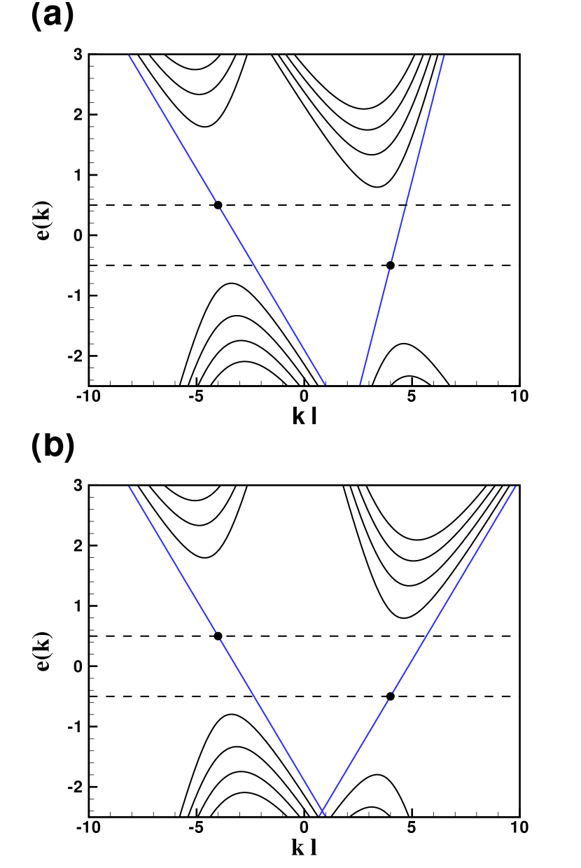
Figure 1: Energy in units of $\hslash v_{F}/\ell$ for the first Landau levels for two nodes with opposite chirality and bias. Parameters are $\chi_{1}=-1,Q_{0,1}\ell=0.5$ for the node on the left and $\chi_{2}=+1,Q_{0,2}\ell=-0.5$ for the node on the right and : (a) $t_{1,z}=t_{2,z}=0.4$ and (b) $t_{1,z}=-t_{2,z}=0.4$. The blue lines and the black dots are the chiral level and Dirac point in each node. The separation between the nodes is arbitrary.

The minimal (maximal) energy in level $n>0$ ($n<0$) is given by

$$\min\left[e_{n>0}\right] = Q_{0}\ell+\sqrt{2\beta\gamma n},$$ (7)

$$\max\left[e_{n<0}\right] = Q_{0}\ell-\sqrt{2\beta\gamma\left|n\right|,}$$ (8)

where we have defined

$$\gamma=1-t^{2}.$$ (9)

These extrema occur at wave vector

$$\left(k\ell\right)_{\text{ext}}=-\text{sgn}(n)\sqrt{\frac{2\left|n\right|\beta}{\gamma}}t_{z}.$$ (10)

The energy bias in real energy units $\Delta_{0}$ is independent of the magnetic field while the unitless energy bias $Q_{0}\ell$ varies with the magnetic field according to the relation

$$Q_{0}\ell=\frac{\Delta_{0}}{\hbar v_{F}/\ell}.$$ (11)

The dispersion $E_{n=0}=\frac{\hslash v_{F}}{\ell}e_{n=0}$ of the chiral level in real energy units is independent of the magnetic field.

II.2 Density of states

At energy $e,$ the level index of the highest partially occupied Landau level in each node is

$$n_{\max}\left(e\right)=\text{sgn}(e-Q_{0}\ell)\lfloor\frac{\left(e-Q_{0}\ell\right)^{2}}{2\beta\gamma}\rfloor,$$ (12)

where $\lfloor\rfloor$ is the floor function.

The density of states (DOS) $g\left(e\right)$ per unit volume $V$ is

$$g\left(e\right) = \frac{1}{V}N_{\varphi}\sum_{n,k}\delta\left(\frac{\hslash v_{F}}{\ell}\left(e-e_{n}\left(k\right)\right)\right)$$

$$= \frac{\alpha}{\beta+\chi t_{z}}$$

$$+\sum_{n=1}^{n_{\max\left(e\right)}}\sum_{j=\pm 1}\frac{\alpha\Theta\left(e-Q_{0}\ell\right)}{\left|t_{z}+\frac{\beta k_{n,j}\ell}{\sqrt{k_{n,j}^{2}\ell^{2}+2\beta n}}\right|}$$

$$+\sum_{n=n_{\max}\left(e\right)}^{-1}\sum_{j=\pm 1}\frac{\alpha\Theta\left(Q_{0}\ell-e\right)}{\left|t_{z}-\frac{\beta k_{n,j}\ell}{\sqrt{k_{n,j}^{2}\ell^{2}+2\beta\left|n\right|}}\right|},$$

where the constant $\alpha$ is defined by

$$\alpha=\frac{1}{4\pi^{2}\ell^{3}}\frac{1}{\hslash v_{F}/\ell}.$$ (14)

(Note that $\beta+\chi t_{z}>0$ for all angles $\theta.$) Each Landau level $\left(n,k\right)$ has a degeneracy given by $N_{\varphi}=S/2\pi\ell^{2},$ where $S$ is the area of the WSM perpendicular to the magnetic field. In Eq. (II.2), the wave vectors $k_{n,\pm}\ell$ are defined by

$$k_{n,\pm}\ell = -\frac{1}{\gamma}\left(e-Q_{0}\ell\right)t_{z}$$

$$\pm\frac{\beta}{\gamma}\sqrt{\left(e-Q_{0}\ell\right)^{2}-2\left|n\right|\beta\gamma}.$$

The $k_{n,\pm}\ell$ are the two $k$ points in each level $n\neq 0$ where $e_{n}\left(k_{n,\pm}\ell\right)=e_{F}$ with $e_{F}$ the unitless Fermi level. At a band extremum, they merge into a single point with wave vector $k_{n,j=\pm}\ell=\left(k_{n}\ell\right)_{\text{ext}}$ given by Eq. (10). At this particular point, the denominator in the third line of Eq. (II.2) goes to zero and the density of states diverges as shown in Fig. 2.

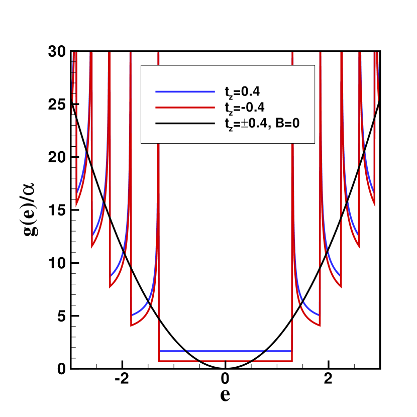
Figure 2: Density of states as a function of the energy $e$ for a single node with zero bias, chirality $\chi=-1$ and for $t_{z}=\pm 0.4.$ The black line is the $B=0,t_{z}=\pm 0.4$ result which does not depend on the sign of $t_{z}$.

At zero tilt and bias, Eq. (II.2) reduces to the known resultCarbotte1 :

$$g\left(e\right)=\alpha\left[1+2\left|e\right|\sum_{n=1}^{\left|n_{\max}\left(e\right)\right|}\frac{1}{\sqrt{e^{2}-2\left|n\right|}}\right],$$ (16)

and at zero magnetic field to:

$$g\left(E\right)=\frac{1}{2\pi^{2}}\frac{\left(E-\Delta_{0}\right)^{2}}{\left(\hslash v_{F}\right)^{3}}\frac{1}{\left(1-t^{2}\right)^{2}},$$ (17)

which is represented by the black line in Fig. 2.

The term in the second line of Eq. (II.2) is the contribution of the chiral level to the density of states. It is independent of the energy but increases linearly with the magnetic field. The density of states depends on the chirality and tilt vector only through the product $\chi t_{z}$ only. As for the contribution of the $n\neq 0$ levels, it can be deduced from Eq. (II.1) and the summation over $k$ in Eq. (II.2) that it is independent of the sign of $t_{z}$ because of the symmetry relation $e_{n\neq 0}\left(k,t_{z},Q_{0}\ell\right)=e_{n\neq 0}\left(-k,-t_{z},Q_{0}\ell\right).$ It is also independent of the chirality index. It is thus convenient to define the density of states for a node as the sum of the two contributions:

$$g\left(e\right)=g_{0,\chi}+g_{>}\left(e-Q_{0}\ell\right),$$ (18)

where $g_{>}\left(e\right)$ is the density of states from levels $n\neq 0$ defined with $Q_{0}=0$ and

$$g_{0,\chi}=\frac{\alpha}{\beta+\chi t_{z}}$$ (19)

is the contribution of the chiral level.

Figure 2 shows the sawtooth behavior of the density of states as a function of the unitless energy $e$ for a single node with zero bias, chirality $\chi=-1$ and for $t_{z}=\pm 0.4.$ The density of states from the chiral level is reduced (increased) from its $t_{z}=0$ value when $\chi t_{z}>0$ ($\chi t_{z}<0).$ Equation (7) shows that the gap between the positive and negative energy levels is reduced by a finite value of $\left|\mathbf{t}\right|$. A finite bias only shifts the function $g\left(e\right)$ globally to $e>0$ $\left(e<0\right)\,$ for $Q_{0}$ positive (negative). The separations between the square root singularities in the density of states scale as $\sqrt{B}$ for a Weyl fermions in contrast with three-dimensional Schrödinger fermions where it increases linearly with the magnetic field.

II.3 Magnetization and magnetic susceptibility

Throughout our paper, we work at $T=0$ K so that the magnetization per electron in units of the Bohr magneton $\mu_{B}=e\hslash/2m_{e}$ (where $m_{e}$ is the bare electron mass) is obtained by taking the derivative of the electronic energy per electron $U$ (which we define below) with respect to the magnetic field at constant density:

$$m=-\frac{1}{\mu_{B}}\left.\frac{\partial U}{\partial B}\right|_{n_{e}}.$$ (20)

Differentiating the energy a second time gives the (differential) magnetic susceptibility per electron in units of Bohr magneton per Tesla:

$$\chi_{m}=-\frac{1}{\mu_{B}}\left.\frac{\partial^{2}U}{\partial B^{2}}\right|_{n_{e}}=\left.\frac{\partial m}{\partial B}\right|_{n_{e}}.$$ (21)

III MAGNETIC SUSCEPTIBILITY FROM A SINGLE WEYL NODE

In this section, we derive the magnetic oscillations from the electrons in a single node. We can set $Q_{0}=0$ in all formulas since shifting the zero of energy (the Dirac point) of a node when its density $n_{e}$ is fixed does not change its magnetization or susceptibility.

III.1 Fermi level and density of carriers

The vacuum state is defined as the filled valence band of the Dirac cone. We define the carrier density with respect to that vacuum state. It is positive for electrons ($e_{F}>0$) and negative for holes $\left(e_{F}<0\right).$ According to Eqs. (7,8), the Fermi level is in the chiral level when $\left|e_{F}\right|<\sqrt{2\beta\gamma}$ and intersects the Landau level $n\neq 0$ when

$$\left|e_{F}\right|\geq\sqrt{2\left|n\right|\beta\gamma}.$$ (22)

The density of carriers is related to the chemical potential by the equation

$$n_{e} = \frac{\hslash v_{F}}{\ell}\int_{0}^{e_{F}}g\left(e\right)de$$

$$= \frac{1}{4\pi^{2}\ell^{3}}\frac{e_{F}}{\chi t_{z}+\beta}$$

$$+\frac{\Theta\left(e_{F}\right)}{4\pi^{2}\ell^{3}}\sum_{n=1}^{n=n_{\max}\left(e_{F}\right)}\Lambda_{n}\left(e_{F}\right)$$

$$-\frac{\Theta\left(-e_{F}\right)}{4\pi^{2}\ell^{3}}\sum_{n=n_{\max}\left(e_{F}\right)}^{n=-1}\Lambda_{n}\left(e_{F}\right),$$

where we have defined

$$\Lambda_{n}\left(e\right) = k_{n,+}\ell\left(e\right)-k_{n,-}\ell\left(e\right)$$

$$= 2\frac{\beta}{\gamma}\sqrt{e^{2}-2\left|n\right|\beta\gamma}.$$

The oscillations of the Fermi level $e_{F}\left(B\right)$ with magnetic field are found by solving Eq. (III.1) with $n_{e}$ fixed. A numerical evaluation shows that, when $B\rightarrow 0,$ Eq. (III.1) reduces to the classical result

$$E_{F}=\text{sgn}\left(n_{e}\right)\hslash v_{F}\left(6\pi^{2}\left(1-t^{2}\right)^{2}\left|n_{e}\right|\right)^{1/3}.$$ (25)

III.2 Electronic energy

At zero temperature, the kinetic energy per carrier is

$$U=\frac{1}{\left|n_{e}\right|}\left(\frac{\hslash v_{F}}{\ell}\right)^{2}\int_{0}^{e_{F}}g\left(e\right)ede.$$ (26)

It is positive for both electron ($n_{e}>0,e_{F}>0$) or hole ($n_{e}<0,e_{F}<0$) carriers. Using the definition of the density of states, the energy becomes

$$U = \frac{1}{2}\zeta\frac{e_{F}^{2}}{\beta+\chi t_{z}}$$

$$+\zeta\Theta\left(e_{F}\right)\sum_{n=1}^{n_{\max}\left(e_{F}\right)}\int_{k_{n,-}\ell\left(e_{F}\right)}^{k_{n,+}\ell\left(e_{F}\right)}e_{n}\left(x\right)dx$$

$$-\zeta\Theta\left(-e_{F}\right)\sum_{n=n_{\max}\left(e_{F}\right)}^{n=-1}\int_{k_{n,-}\ell\left(e_{F}\right)}^{k_{n,+}\ell\left(e_{F}\right)}e_{n}\left(x\right)dx,$$

where we have defined

$$\zeta=\frac{\hslash v_{F}/\ell}{4\pi^{2}\left|n_{e}\right|\ell^{3}}=0.385\frac{B^{2}}{\left|\overline{n}_{e}\right|}\overline{v}_{F}\text{ (meV)}$$ (28)

We define $\overline{n}_{e}$ and $\overline{v}_{F}$ as the unitless carrier density and Fermi velocity by $n_{e}=\overline{n}_{e}\times 10^{22}$ m^-3 and $v_{F}=\overline{v}_{F}\times 10^{5}$ m/s. In our numerical calculation, we use $\overline{v}_{F}=3$ and $\overline{n}_{e}=2$. For comparison, in the Weyl semimetal TaAs, $\overline{v}_{F}\approx 3.6$ and $\overline{n}_{e}\approx 0.42$ for the W1 nodes and $\overline{n}_{e}\approx 0.00105$ for the W2 nodes.

The integrals in Eq. (III.2) can be evaluated analytically to give

$$\int e_{n}\left(x\right)dx = \frac{1}{2}x^{2}t_{z}$$

$$+\frac{1}{2}\text{sgn}(n)\beta x\sqrt{x^{2}+2\beta\left|n\right|}$$

$$+\beta^{2}n\ln\left(x+\sqrt{x^{2}+2\beta\left|n\right|}\right).$$

Equation (III.2) reduces to the energy result given by Eq. (33) of Ref. (Carbotte1, ) calculated in the absence of tilt and bias. At equal density, the energy $U$ is the same for electron and hole carriers. The magnetization and susceptibility are then also the same and we can, without loss of generality, consider only electron carriers for the rest of this section.

Figure 3 shows an example of quantum oscillations of the magnetic susceptibility and magnetization for $\chi=\pm 1,t_{z}=0,\pm 0.4$ and $\overline{n}_{e}=2.$ The oscillations are identical for two nodes with the same sign of the product $\chi t_{z}$. For the susceptibility (magnetization), they increase (decrease) in amplitude as $1/B$ increases. Each discontinuity in the slope of the oscillations indicates a transition of the Fermi level from $n$ to $n+1$ if $1/B$ increases. At high magnetic field, the WSM enters the quantum regime where the Fermi level intersects only the chiral level. In this regime, the magnetization is positive and increases as $1/B^{2}$ while the susceptibility increases as $1/B^{3}$ (see below where we derive these results). We denote the critical magnetic field where the WSM enter the quantum limit by $B_{1}$ and study its behavior in the next section.

To see the importance of the chiral level, we show (the green curve in Fig. 3) the behavior of the susceptibility when the chiral level is artifically removed from the calculation. Note that, in this case, the first discontinuity near $1/B\approx 0.4$ T^-1 corresponds to the transition of the Fermi level from $n=1$ to $n=2$ and not from $n=0$ to $n=1$ as in real WSM. With no chiral level, the oscillations are phase shifted with respect to those of a real WSM. Their large $B$ behavior is also different. Without the chiral level, the susceptibility is positive instead of negative at large $B$ as shown in the inset of Fig. 3. Moreover, at large $B,$ the electrons condense at the bottom of the $n=1$ level so that the susceptibility $\chi_{m}\sim B^{3/2}$. The large $B$ behavior of $\chi_{m}$ in the WSM can also be contrasted with that of the three-dimensional Schrödinger fermions where $\chi_{m}$ $\sim B^{-4}$.

The magnetization goes to zero at small $B$ in the absence of a tilt as expected on physical grounds. When $\chi t_{z}<0,$ however, the magnetization tends to a constant positive value $m_{0}$ at small $B$ and inversely if $\chi t_{z}>0$ where it tends to $-m_{0}.$ In all cases, however, the magnetization due to the added carriers increases linearly with $B$ at small $B$ and the magnetic susceptibility $\chi=dm/dB>0.$ The response is paramagnetic. For a WSM with two nodes of opposite chirality, the minimal number of nodes required by the Nielsen-Ninomiya theoremNielsen , both nodes would need to have the same tilt in order for the magnetization to vanish in the $B\rightarrow 0$ limit. This is not possible, however, if inversion symmetry is to be preserved since opposite tilts are then required. There would thus be a spontaneous magnetization in this case. To preserve time-reversal symmetry, at least four nodes are required and the summation of $\chi t_{z}$ over these nodes gives zero hence no spontaneous magnetization. This spontaneous magnetization has been discussed before (see Ref. Mikitik2019, ).

We can consider a Dirac node as two Weyl points of opposite chiralities but with the same tilt located at the same wave vector $\mathbf{k}_{0}$ in the Brillouin zone. From the previous paragraph, the spontaneous magnetization is then zero for a Dirac node. A Dirac node has two chiral levels ($n=0$) with opposite chiralities and the Landau levels $n\neq 0$ are twofold degenerate in spin. Apart from this degeneracy, these $n\neq 0$ levels have the same dispersion than the Landau levels in a Weyl node (assuming no energy bias). The Weyl node, however, has only one chiral level. The different behavior with respect to the spontaneous magnetization thus comes from the chiral level i.e. from the first term on the right-hand side of Eq. (III.2). For a Weyl node, the energy of the electron gas in the $n=0$ level is $U_{W}=\zeta\frac{e_{F}^{2}/2}{\beta+\chi t_{z}}$ while for a Dirac node it is $U_{D}=\zeta\frac{e_{F}^{2}/2}{\beta+\chi t_{z}}\left(\frac{1}{\beta+\chi t_{z}}+\frac{1}{\beta-\chi t_{z}}\right).$ We can write

$$U_{W}=\frac{1}{2}U_{D}-\frac{1}{2}\chi t_{z}\zeta\frac{e_{F}^{2}/2}{\beta^{2}-t_{z}^{2}},$$ (30)

so that the magnetization of a Weyl node is half that of a Dirac node but with a correction that depends on the product $\chi t_{z}.$ (We recover in this way Eq. (36) of Ref. Mikitik2019, .)

To obtain the magnetization of the WSM and not just that of the added carriers, one must also consider the contribution of the filled states in the valence band (the vacuum). This contribution has been studied in a number of papers (for a review, see Ref. Mikitik2019, ). It is found that the occupied states in the valence band are responsible for a giant diamagnetic anomaly in the magnetic susceptibility which diverges as the Fermi level goes to zero when $B\rightarrow 0$ i.e. $\chi_{m}\sim-\ln\left(\frac{E_{c}}{E_{F}}\right),$ where $E_{c}$ is a high-energy cutoff. Moreover, it has been shownCarbotte1 that, at zero tilt, the vacuum gives a negative contribution to the magnetization which is linear in $B$ and so a negative contribution to the magnetic susceptibility. It does not contribute to the magnetic oscillations, however. At the opposite, in the extreme quantum limit where the magnetization due to the added carriers goes to zero, the vacuum diamagnetic response will dominate the response of the Weyl semimetal, giving a magnetization that increases without limit as $B$ increases. This is the so-called magnetic torque anomalyMoll . (See also the last paragraph in Sec. III where we comment more on this point.)

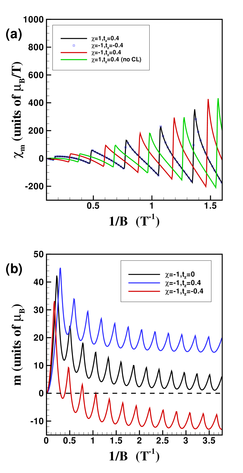
Figure 3: (a) Magnetic susceptibility at zero bias from a single node for different chiralities and sign of the $z$ component of the tilt vector. The green line is for a node where the chiral level has been artifically removed. The large $B$ behavior is shown in the inset. (b) Magnetisation for a node with chirality -1 and tilt vector $t_{z}=0,0.4,-0.4$ showing the different behaviors in the small $B$ limit.

III.3 Behavior of $B_{1}$ and the quantum limit

For a single node with chirality $\chi$ and tilt $\mathbf{t}$ filled with a density of electrons $n_{e},$ the peaks in the oscillations of the physical quantities occur each time the Fermi energy is at the bottom of an energy level $n>0$ i.e. whenever $e_{F}=\min\left[e_{n>0}\right].$ From Eq. (III.1), the magnetic field at these particular values is given by:

$$\frac{1}{B_{n}}=\kappa\left(\mathbf{t}\right)F\left(n\right),$$ (31)

where we have defined the function

$$F\left(n\right)=\left[\frac{\sqrt{n}}{\chi t_{z}+\beta}+\frac{2\beta}{\gamma}\sum_{n^{\prime}=1}^{n^{\prime}=n-1}\sqrt{n^{\prime}}\right]^{2/3}$$ (32)

and the parameter

$$\kappa\left(\mathbf{t}\right)=\left(\frac{e}{\hslash}\right)\left(\frac{\left(2\beta\gamma\right)^{1/2}}{4\pi^{2}n_{e}}\right)^{2/3}=0.356\frac{\left(\beta\gamma\right)^{1/3}}{\overline{n_{e}}^{2/3}}.$$ (33)

In particular, the transition of the Fermi level from the chiral level to $n=1$, i.e. the transition to the quantum limit, occurs at a magnetic field $B_{1}$ given by

$$\frac{1}{B_{1}} = \kappa\left(\mathbf{t}\right)\frac{1}{\left(\chi t_{z}+\beta\right)^{2/3}}$$

$$= \frac{0.356}{\left(\overline{n_{e}}\right)^{2/3}}\Upsilon\left(t,\theta\right)$$

where we have defined the function

$$\Upsilon\left(t,\theta\right)=\frac{\left(\left(1-t^{2}\right)\sqrt{1-t^{2}\sin^{2}\theta}\right)^{1/3}}{\left(\chi t\cos\theta+\sqrt{1-t^{2}\sin^{2}\theta}\right)^{2/3}}.$$ (35)

The quantum limit is reached at a smaller $B$ field when the density is decreased. The angular dependence of the function $\Upsilon$ is shown in Fig. 4 for tilts $t=0$ and $t_{z}=0.4$ and for the two chiralities. There is no angle dependence at zero tilt. The field $B_{1}$ can be measured by torque magnetometry experimentsMoll .

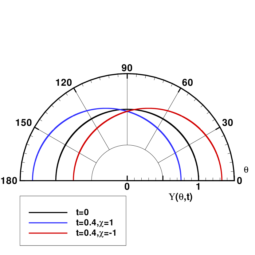
Figure 4: Angular dependence $\Upsilon\left(t,\theta\right)$ of $1/B_{1}$ for tilts $t=0$ and $t_{z}=0.4$ and both chiralities.

III.4 Periodicity of the oscillations in the $B\rightarrow 0$ limit

If $B_{n}$ is the magnetic field where the Fermi level is just below level $n$ and $B_{n+1}$ where it is just below $n+1,$ then the separation between two discontinuities in the slope of the oscillations is given by

$$P\left(\mathbf{t},n\right) \equiv \frac{1}{B_{n+1}}-\frac{1}{B_{n}}$$ (36)

$$= \kappa\left(\mathbf{t}\right)\left[F\left(n+1\right)-F\left(n\right)\right],$$

in units of Tesla${}^{-1}.$ Figure 5 shows that $P\left(\mathbf{t},n\right)$ depends on $n.$ The oscillations contain multiple Fourier components in $1/B,$ they are not periodic in $1/B$ in contrast with the oscillations from two-dimensional Schrödinger fermions. For large $n,$ however, Fig. 5 indicates that $P\left(\mathbf{t},n\right)$ is constant and we can write in this limit:

$$\lim_{n\rightarrow\infty}F\left(n+1\right)-F\left(n\right)\rightarrow 2\left(\frac{2}{9}\right)^{1/3}\left(\frac{2\beta}{\gamma}\right)^{2/3}.$$ (37)

It is thus possible to define a period (in units of Tesla^-1) in this small $B$ limit by

$$\lim_{n\rightarrow\infty}P\left(t,\theta,n\right) = 2\left(\frac{2}{3}\right)^{2/3}\frac{e}{\hslash}$$

$$\times\left(\frac{1}{4\pi^{2}n_{e}}\right)^{2/3}\Gamma\left(t,\theta\right)$$

$$= 0.430\,89\left(\frac{1}{\overline{n_{e}}}\right)^{2/3}\Gamma\left(t,\theta\right),$$

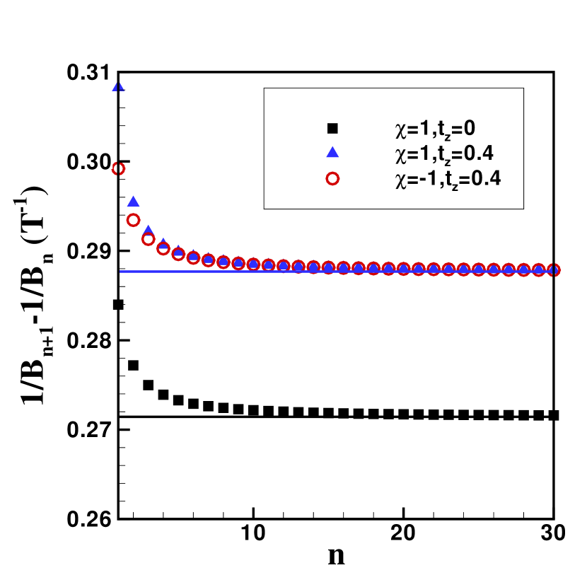
Figure 5: The function $P\left(\mathbf{t},n\right)$ as a function of $n$ for different values of the chirality and tilt. The full lines gives the limit $\lim_{n\rightarrow\infty}P\left(\mathbf{t},\chi,n\right).$

$$\Gamma\left(t,\theta\right)=\frac{\sqrt{1-t^{2}\sin^{2}\theta}}{\left(1-t^{2}\right)^{1/3}}$$ (39)

shows the anisotropy of the period. In the absence of tilt, this period $P$ is precisely that given by the dominant oscillatory term in the Poisson formula for the magnetizationCarbotte1 [if the chemical potential in Eq. (38) of this reference is replaced by the $B=0$ result given by our Eq. (25)]. With a tilt along $z,$ the Fermi surface becomes ellipsoidal instead of spherical and $\lim_{n\rightarrow\infty}P\left(t,\theta=0,n\right)=2\pi e/\hslash S$ is nothing but the usual De Haas-Van Alphen period with $S$ the area in $\mathbf{k}$ space of the maximal orbit for $\mathbf{B}$ along the $z$ direction. This period does not depend on the chirality or on the sign of the tilt component $t_{z}$ or on the Fermi velocity. It has the angular dependence shown in Fig. 6.

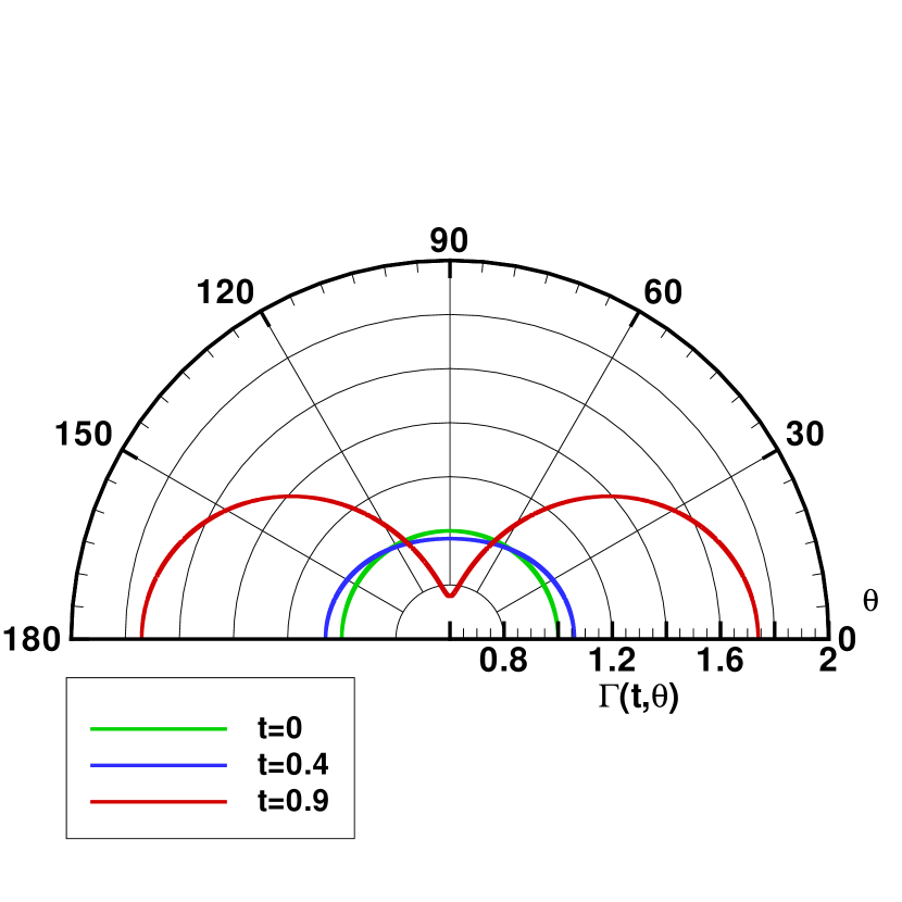
Figure 6: Angular dependence of the function $\Gamma\left(\mathbf{t},\theta\right)$ entering in the fundamental period of the magnetic oscillations.

It is interesting to compare Eq. (31) with the corresponding results for three-dimensional Schrödinger’s fermions which have the dispersion

$$E_{n}=\left(n+\frac{1}{2}\right)\hslash\omega_{c}+\frac{\hslash^{2}k^{2}}{2m_{e}},$$ (40)

with $m_{e}$ the electron mass and $\omega_{c}=eB/m_{e}$ the cyclotron frequency. A calculation following exactly the same steps as above gives in the Schrödinger case:

$$\frac{1}{B_{n,S}}=2\frac{e}{\hslash}\left(\frac{1}{4\pi^{2}n_{e}}\right)^{2/3}\left(\sum_{n^{\prime}=1}^{n}\sqrt{n^{\prime}}\right)^{2/3}$$ (41)

while for Weyl fermions with no tilt

$$\frac{1}{B_{W,n}}=2\left(\frac{e}{\hslash}\right)\left(\frac{1}{4\pi^{2}n_{e}}\right)^{2/3}\left[-\frac{1}{2}\sqrt{n}+\sum_{n^{\prime}=1}^{n}\sqrt{n^{\prime}}\right]^{2/3}.$$ (42)

In the large $n$ limit, both expressions give the same period for the oscillations, namely (setting $t=0$ for the Weyl node)

$$\lim_{n\rightarrow\infty}P\left(n\right)=2\left(\frac{2}{3}\right)^{2/3}\frac{e}{\hslash}\left(\frac{1}{4\pi^{2}n_{e}}\right)^{2/3}.$$ (43)

Moreover, in the large $n$ limit, we find the relation

$$\frac{1}{B_{n,S}}\approx\frac{1}{2}\left[\frac{1}{B_{n+1,W}}+\frac{1}{B_{n,W}}\right],$$ (44)

so that the Schrödinger and Weyl oscillations are out of phase by half a period as pointed out in Ref. Carbotte1, .

III.5 Magnetization and susceptibility in the quantum limit

The quantum limit is reached when the magnetic field is such that the Fermi level intersects only the chiral level i.e. $e_{F}\in\left[0,\min\left[e_{1}\right]\right]$ for electron or $e_{F}\in\left[\max\left[e_{-1}\right],0\right]$ for holes. From Eq. (III.1), the Fermi level is then given by

$$e_{F}=4\pi^{2}\ell^{3}n_{e}\left(\chi t_{z}+\beta\right).$$ (45)

It asymptotically approaches the neutrality point $e_{F}\rightarrow 0$ at large $B$. With this expression in Eq. (III.2), the energy per carrier in this limit is given by

$$U=\frac{\left|n_{e}\right|h^{2}v_{F}}{2eB}\left(\chi t_{z}+\beta\right)$$ (46)

and so the magnetization and susceptibility per carrier are given by

$$m=\frac{\left|n_{e}\right|h^{2}v_{F}}{2\mu_{B}eB^{2}}\left(\chi t_{z}+\beta\right)$$ (47)

and

$$\chi_{m}=-\frac{\left|n_{e}\right|h^{2}v_{F}}{\mu_{B}eB^{3}}\left(\chi t_{z}+\beta\right).$$ (48)

The magnetization of Weyl electrons is positive in this limit (since $\chi t_{z}+\beta>0$) a behavior observed in the Weyl semimetal NbAs for exampleMoll . It also goes to zero as $B\rightarrow\infty.$ This contrasts with the behavior of Schrödinger electrons in the quantum limit where the magnetization per electron goes to the negative value $m=-1$ (in units of $\mu_{B}$) at large $B.$

The susceptibility increases or decreases with respect to its value at zero tilt depending on the sign of the product $\chi t_{z}.$ As we pointed out above, one can show in the strong magnetic field limit that for a Weyl semimetal the susceptibility $\chi_{m}\sim 1/B^{3/2}$ if the chiral level is removed (see Fig. 3) while $\chi_{m}\sim-1/B^{4}$ for three-dimensional Schrödinger fermions and $\chi_{m}\sim 1/B^{3}$ for Weyl fermions.

We remark that Eqs. (47-48) are obtained by differentiating the energy (or equivalently the Helmholtz free energy at $T=0$ K) with respect to the magnetic field keeping the density constant. Differentiation of the grand potential $\Omega$ at constant Fermi energy (or chemical potential at $T=0$ K) gives, instead, in the extreme quantum limit,

$$m=\frac{1}{2}\frac{eE_{F}^{2}}{h^{2}v_{F}\mu_{B}\left(\chi t_{z}+\beta\right)}$$ (49)

for the magnetization (in units of Bohr magneton per volume) and the susceptibility is

$$\chi_{m}=0.$$ (50)

Thus, when the Fermi level is kept constant and the WSM enters the extreme quantum limit, the magnetic susceptibility goes to zero and the filled states in the valence band dominate the magnetic response.

IV  QUANTUM OSCILLATIONS FROM TWO WEYL NODES

The Nielsen-Ninomiya theoremNielsen requires that the number of Weyl points in the Brillouin zone be even so that Weyl nodes must occur in pairs of opposite chirality. For simplicity, we analyse the quantum oscillations due to a pair of nodes of opposite chirality and bias but with the same tilt modulus $\left|\mathbf{t}\right|.$ We compute the total magnetization and susceptibility for the two cases $t_{z,1}=\pm t_{z,2}$ (but the same value of $t_{\bot}$). We name these two cases WSM1 and WSM2. Their parameters are defined in Tab. 1. In both cases, $\beta_{1}=\beta_{2}=\beta;\;\gamma_{1}=\gamma_{2}=\gamma$ where the subscript here is the node index. For the numerical calculations, we take $n_{e}=2\times 10^{22}$ m^-3 for the total electronic density and $v_{F}=3\times 10^{5}$ m/s for the Fermi velocity. We define $t_{z}$ and $\Delta_{0}$ as positive. The energy scale is set by

$$\frac{\hslash v_{F}}{\ell}=7.\,\allowbreak 70\sqrt{B}\,\text{meV.}$$ (51)

WSM1	WSM2
$\chi_{1}=-\chi_{2}=1$	$\chi_{1}=-\chi_{2}=1$
$t_{z,1}=t_{z,2}=t_{z}$	$t_{z,1}=-t_{z,2}=t_{z}$
$\Delta_{0,1}=-\Delta_{0,2}=\Delta_{0}$	$\Delta_{0,1}=-\Delta_{0,2}=\Delta_{0}$

Table 1: Parameters for the two-node Weyl semimetals 1 and 2.

We implicitly assume that the bias is not too large so that the two Weyl nodes have separate Fermi surface. In real system, if the Fermi level lies too far from the Dirac point, the two surfaces may merge into one surface that encompasses both nodes.

If there were no scattering between the nodes, we would compute the common Fermi level for some initial magnetic field $\mathbf{B}$ and find the corresponding density of electrons in each node. Then as the magnetic field is increased or decreased to study the quantum oscillations, the Fermi level of the two nodes would differ but the electron density in each node will not change. At large $B,$ the Fermi level $E_{F,i}$ in node $i$ will approach the its neutrality point. Thus, for independent nodes, the total susceptibility would simply be the sum of the susceptibility of each node.

For dependent nodes, scattering at finite temperature will modify the density in each node so that they will always share the same Fermi level as the magnetic field changes. In our calculations, we assume a finite doping so that $E_{F}>\Delta_{0}$ initially. Upon increasing the magnetic field, the common Fermi level can eventually cross the neutrality point in the node with the positive bias thus creating holes in that node (i.e. a negative electron density). The total density of electrons, however, must remain constant. We study the case of dependent nodes which is the real physical situation, for the rest of this section. We assume electron doping, i.e. $n_{e}>0.$

If the two nodes of WSM1 are located at the same wave vector, $\mathbf{k}_{0},$ and if there is no energy bias, then WSM1 can be considered as a node of a Dirac semimetal while WSM2 (with the two nodes located at $\pm\mathbf{k}_{0}$) represent a Weyl semimal with space inversion symmetry. As we mentionned above, at zero energy bias, the distinction between the two metals as regards their magnetic behavior comes from the difference in the chiral level.

IV.1 Density of states and ground state energy

Using Eqs. (18-19), the density of states for the two nodes in WSM1 and WSM2 can be written as

$$g_{1}\left(e\right) = g_{0,+}+g_{0,-}$$

$$+g_{>}\left(e-Q_{0}\ell\right)+g_{>}\left(e+Q_{0}\ell\right),$$

$$g_{2}\left(e\right) = 2g_{0,+}+g_{>}\left(e-Q_{0}\ell\right)+g_{>}\left(e+Q_{0}\ell\right).$$ (53)

They differ by the constant

$$g_{1}\left(e\right)-g_{2}\left(e\right)=g_{0,-}-g_{0,+}=\frac{2\alpha t_{z}}{1-t^{2}}.$$ (54)

A finite tilt $t_{z}$ increases the density of states in WSM1 and decreases it in WSM2. The difference between the two densities of states increases rapidly with $t_{z}$. Figure 7 shows the two densities of states for $Q_{0}\ell=0.5$ and $t_{z}=0.6$ and a fixed magnetic field. Note that the gap $\Delta e$ between the peaks at $n=-1$ and $n=1$ decreases as $\Delta e=2\sqrt{2}-2Q_{0}\ell$ with increasing bias. Equation (7) shows that the position in energy of the peaks in the density of states does not depend on the chirality or sign of $t_{z}$ so that both densities of states have the same structure in energy at any bias, apart from the shift due to the chiral Landau level.

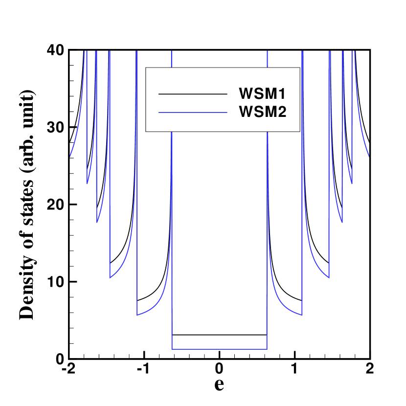
Figure 7: Density of states for the two WSMs for bias $Q_{0}\ell=0.5$ and tilt $t_{z}=0.6.$

The Fermi level for either WSM is found by solving the equation

$$n_{e}=\frac{\hslash v_{F}}{\ell}\int_{Q_{0}\ell}^{e_{F}}g_{1}\left(e\right)de+\frac{\hslash v_{F}}{\ell}\int_{-Q_{0}\ell}^{e_{F}}g_{2}\left(e\right)de,$$ (55)

and the total energy per electron is then given by

$$U = \frac{1}{n_{e}}\left(\frac{\hslash v_{F}}{\ell}\right)^{2}\int_{Q_{0}\ell}^{e_{F}}g_{1}\left(e\right)ede$$

$$+\frac{1}{n_{e}}\left(\frac{\hslash v_{F}}{\ell}\right)^{2}\int_{-Q_{0}\ell}^{e_{F}}g_{2}\left(e\right)ede.$$

IV.2 Magnetic oscillations at zero tilt and finite bias

Figure 8 shows the oscillations in the Fermi level, node density, magnetization and susceptibility, for different values of the bias, when $t=0$ in which case there is no difference between the two WSMs and the magnetization goes to zero at $B=0.$

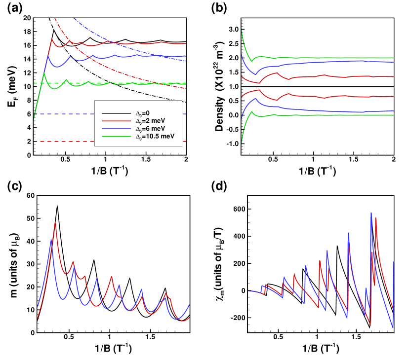
Figure 8: Quantum oscillations as a function of the inverse magnetic field for a WSM with zero tilt and for different values of the bias $\Delta_{0}:$ (a) Fermi level, (b) node densities, (c) magnetization and (d) magnetic susceptibility. The dashed lines in (a) are set at the different values of $\Delta_{0}.$ The density is $n_{e}=2\times 10^{22}$ m${}^{-3}.$

As was the case for a single node, the discontinuities in the quantum oscillations occur every times the magnetic field is such that the chemical potential reaches the minimum of an energy band, i.e. whenever the condition

$$e_{F}\left(B_{n}\right)=\min\left[e_{n>0,\tau}\right]=Q_{0,\tau}\ell+\sqrt{2\beta_{\tau}\gamma_{\tau}n}$$ (57)

is satisfied for a given node $\tau$ and Landau level $n.$ The corresponding magnetic field $B_{n}$ is found by solving

$$n_{e} = \frac{\hslash v_{F}}{\ell}\int_{Q_{0}\ell}^{\min\left[e_{n>0,\tau}\right]}g_{1}\left(e\right)de$$

$$+\frac{\hslash v_{F}}{\ell}\int_{-Q_{0}\ell}^{\min\left[e_{n>0,\tau}\right]}g_{2}\left(e\right)de,$$

where $e_{n>0,\tau}$ in the integration limit is an energy level of either node since the Fermi level passes through many of them as the magnetic field is varied.

In our calculation, we choose the density and bias such that the Fermi level always satisfy $e_{F}>\max\left[e_{n=-1,1}\right]$ so that we do not need to consider the possibility that Landau levels $n\leq-1$ in node $1$ may be occupied with holes. Holes may be present in the chiral level of node $1,$ however, when electrons are transferred to node 2. This happens when the Fermi level $E_{F}$ drops below $\Delta_{0}$, a situation that occurs at $\Delta_{0}=10.5$ meV in Fig. 8(a). There is correspondingly a negative density of electrons in node 1 as can be seen in the panel (b) of this figure. The first peak in $1/B$ in Fig. 8(c) corresponds to $1/B_{1}$ for node $2$ for which $\Delta_{0}<0.$ This node has the largest density of electrons and so reaches the quantum limit at a higher magnetic field. The dashed lines in pannel (a) give the position of the Dirac point in the left node while the dashed-dotted lines indicate the energy of the Landau level $n=1,$ in the left node, below which the Fermi level enters the quantum limit. For $\Delta_{0}=10.5$ meV, this node is always in the quantum limit and the oscillations are due to the electrons in the second node. The doubling of the peaks in panel (a) for $\Delta_{0}=2$ meV is a clear indication that the system has not reached the quantum limit in either node.

The pattern of oscillation changes if we include a tilt of the Weyl nodes in addition to the bias and if we consider the nodes as independent instead of as sharing a common Fermi level. We show an example of the difference between dependent and independent nodes in Fig. 9 for WSM1 with bias $\Delta_{0}=2$ meV and tilt vector $t_{z}=0.5.$ In the independent case, we calculate the initial position of the Fermi level at $B=0.5$ T, assuming an equilibrium between the two nodes at that initial field. We assume the same total density $n_{e}=2\times 10^{22}$ m^-3 in both cases.

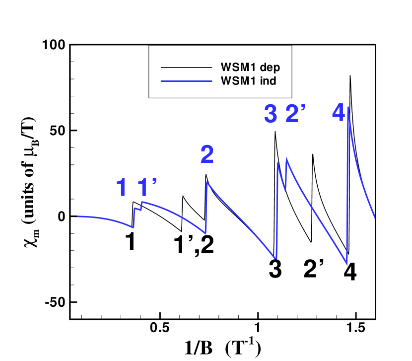
Figure 9: Susceptibility per carrier calculated for WSM1 for dependent and independent nodes assuming the same total density $n_{e}=2\times 10^{22}$ m^-3 , bias $\Delta_{0}=2$ meV and tilt $t_{z}=0.5.$ The number above or below each peak indicates the Landau level that is crossed by the Fermi level. Black (blue) numbers are for dependent (independent) nodes and $n(n^{\prime})$ stand for node $2(1).$ Node 1(2) is shifted upward(downward) in energy (see Table 1).

The difference between dependent and independent nodes is more pronounced when the WSM is compensated i.e. when there is initially an equal number of electrons and holes. If the nodes are dependent, the Fermi level will not move with a variation of the magnetic field since $n_{e}=0$ and so the susceptibility will be zero (see Eqs. (67-68) below). For WSM1, the Fermi level will be lying between $-\Delta_{0}$ and $+\Delta_{0}$ since $\left|t_{z}/\beta\right|<1$ while for WSM2, it will be exactly at $E_{F}=0.$ For independent nodes, the susceptibility of each node does not depend on the sign of the carrier and the susceptibility will be twice that of a single node for the susceptibility per volume.

IV.3 Quantum limit at finite tilt and bias

The quantum limit is reached when the Fermi level is in the chiral level of both nodes. When this occurs, the behavior of the Fermi level with the magnetic field is given by

$$E_{F,\text{WSM1}} = \frac{h^{2}v_{F}n_{e}\gamma}{2\beta e}\frac{1}{B}-\frac{\Delta_{0}t_{z}}{\beta},$$ (59)

$$E_{F,\text{WSM2}} = \frac{h^{2}v_{F}n_{e}\left(\beta+t_{z}\right)}{2e}\frac{1}{B},$$ (60)

and is linear in $1/B$ as shown in Fig. 8(a). When $B$ is very large $E_{F,\text{WSM1}}\rightarrow-\frac{\Delta_{0}t_{z}}{\beta}$ and $E_{F,\text{WSM2}}\rightarrow 0$ i.e. the Fermi level asymptotically approaches the neutrality point of each WSM. At zero tilt, $E_{F}\rightarrow 0$ for both WSMs at large $B,$ in contrast to the case of independent nodes (no scattering) where the Fermi level in each node approaches the corresponding neutrality point $\pm\Delta_{0.}$

The total energy per carrier is given in this limit by

$$U_{WSM1} = \frac{1}{2}\zeta\frac{e_{F}^{2}-\left(Q_{0}\ell\right)^{2}}{\beta+t_{z}}+\frac{1}{2}\zeta\frac{e_{F}^{2}-\left(Q_{0}\ell\right)^{2}}{\beta-t_{z}}$$

$$= \frac{ev_{F}}{4\pi^{2}n_{e}}\frac{1}{\beta}$$

$$\times\left(\frac{4\pi^{4}\hslash^{2}n_{e}^{2}\gamma}{e^{2}B}-\frac{4\pi^{2}\hslash n_{e}Q_{0}t_{z}}{e}-BQ_{0}^{2}\right)$$

and

$$U_{WSM2} = \frac{1}{2}\zeta\frac{e_{F}^{2}-\left(Q_{0}\ell\right)^{2}}{\beta+t_{z}}+\frac{1}{2}\zeta\frac{e_{F}^{2}-\left(Q_{0,\tau}\ell\right)^{2}}{\beta+t_{z}}$$

$$= \frac{1}{2}\frac{ev_{F}}{4\pi^{2}n_{e}}\left(\frac{2}{\beta+t_{z}}\right)$$

$$\times\left(\frac{4\pi^{4}\hslash^{2}n_{e}^{2}\left(\beta+t_{z}\right)^{2}}{e^{2}B}-BQ_{0}^{2}\right).$$

Equations (20,21) give for the magnetization per carrier

$$m_{WSM1} = \frac{h^{2}n_{e}v_{F}}{4\mu_{B}eB^{2}}\frac{\gamma}{\beta}+\frac{e}{\mu_{B}h^{2}n_{e}v_{F}}\frac{\Delta_{0}^{2}}{\beta},$$ (63)

$$m_{WSM2} = \frac{h^{2}n_{e}v_{F}}{4\mu_{B}eB^{2}}\left(\beta+t_{z}\right)$$

$$+\frac{e}{\mu_{B}h^{2}n_{e}v_{F}}\frac{\Delta_{0}^{2}}{\beta+t_{z}},$$

and for the susceptibility per carrier

$$\chi_{m,WSM1} = -\frac{h^{2}n_{e}v_{F}}{2\mu_{B}eB^{3}}\frac{\gamma}{\beta},$$ (65)

$$\chi_{m,WSM2} = -\frac{h^{2}n_{e}v_{F}}{2\mu_{B}eB^{3}}\left(\beta+t_{z}\right).$$ (66)

When the Fermi level is in the chiral level of node 2, the susceptibility of the two WSMs are independent of the bias. Moreover, the two WSMs then differ only in their dependence on the tilt direction which is given by

$$\chi_{m,WSM1} \sim \left(1-t^{2}\right)/\sqrt{1-t^{2}\sin^{2}\theta},$$ (67)

$$\chi_{m,WSM2} \sim \sqrt{1-t^{2}\sin^{2}\theta}+t\cos\theta.$$ (68)

The $1/B^{2}$ behavior of the magnetization is clearly visible in Fig. 8(c). When only the chiral level is occupied, our calculation shows that the susceptibility is negative at large $B$ and there is a constant contribution to the magnetization at finite bias. This constant is very small. At zero tilt, for example, it is given by

$$m=\frac{e\Delta_{0}^{2}}{\mu_{B}h^{2}n_{e}v_{F}}=8.\,\allowbreak 528\,5\times 10^{-3}\frac{\overline{\Delta}_{0}^{2}}{\overline{n_{e}}}$$ (69)

in Bohr magneton per electron.

IV.4 Behavior of $B_{1}$ and periodicity of the oscillations at finite tilt and bias

The first peak at small $1/B$ occurs when the Fermi level $e_{F}\left(B\right)=\min\left[e_{1,2}\right]$ i.e. when the system enters the quantum limit. It is then in the chiral level of both nodes so that only the contribution to the density of states of these levels need to be considered. The magnetic lengths $\ell_{1}$ and $\ell_{2}$ (corresponding to $1/B_{1}$) for WSM1 and WSM2 are given by solving the equations

$$\ell_{1}^{3}+\frac{Q_{0}}{\xi}\ell_{1}-\frac{1}{2\pi^{2}n_{e}}\sqrt{\frac{2\beta^{3}}{\gamma}} = 0,$$ (70)

$$\ell_{2}^{3}+\frac{Q_{0}}{\xi}\ell_{2}-\frac{\sqrt{2\beta\gamma}}{\xi} = 0,$$ (71)

where $Q_{0}\geq 0$ and we have defined the constant

$$\xi=2\pi^{2}n_{e}\left(\beta+t_{z}\right).$$ (72)

If there is no tilt, the magnetic length at this peak is instead given by the solution of the equation

$$\ell_{0}^{3}+\frac{Q_{0}}{2\pi^{2}n_{e}}\ell_{0}-\frac{1}{\sqrt{2}\pi^{2}n_{e}}=0.$$ (73)

In particular, at zero bias the position in $1/B$ of the first peak is

$$\frac{1}{B_{1}}=0.564\,62\frac{1}{\overline{n}_{e}^{2/3}}\text{ T}^{-1},$$ (74)

which is simply Eq. (III.3) with a electronic density $n_{e}/2.$

IV.5 Magnetic oscillations and quantum limit at zero bias

Figure 10 shows the effect of a finite $t_{z}$ on the magnetic susceptibility and magnetization of both WSMs for zero bias. The spacing between the oscillations increases with $t_{z}$ for both WSMs while it decreases with a finite $t_{\bot}$ (not shown in the figure). The susceptibility decreases with $t_{z},$ more so for WSM2 than for WSM1. As discussed in Sec. III, the magnetization does not go to zero at small $B$ for WSM2 since the two nodes have $\chi t_{z}=1$.

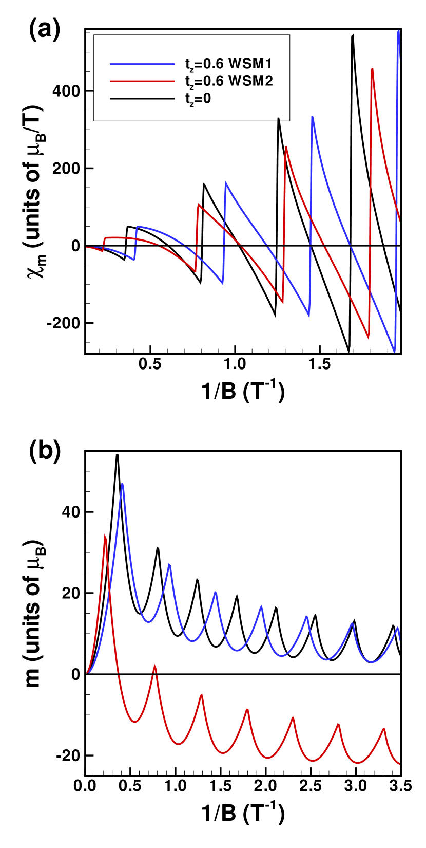
Figure 10: Effect of a finite tilt on (a) the magnetic susceptibility and (b) magnetization of both WSMs at zero bias.

At zero bias, Eq. (III.4) can be generalized for WSM2 (opposite tilts) to

$$\lim_{n_{0}\rightarrow\infty}\lambda\left(\mathbf{t},n_{0}\right)=2\left(\frac{2}{3}\right)^{4/3}\frac{e}{\hslash}\left(\frac{1}{4\pi^{2}n_{e}}\right)^{2/3}\left(\frac{\beta}{\gamma^{1/3}}\right),$$ (75)

taking into account that, in this case, the node density is $n_{e}/2.$

Figure 11 shows $1/B_{1}$ for both WSMs as a function of the polar angle $\theta$ for different values of the bias $\Delta_{0}$ and tilt modulus $t.$ If there is no tilt, there is no distinction between the two WSMs at any bias. For a finite tilt, $1/B_{1}$ (WSM1)$>1/B_{1}$ (WSM2) if $t_{z}>0$ (i.e. $\theta<\pi/2$) and vice versa. Both peaks are shifted to lower values of $1/B$ by a finite bias. A finite tilt thus introduces a dephasing that is different for the two Weyl semimetals and which is also anisotropic.

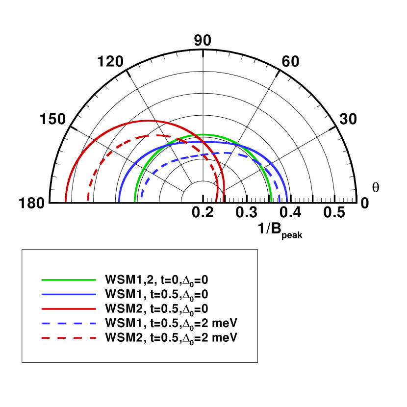
Figure 11: Position of the first peak in $1/B$ of the quantum oscillations for WSM1 and WSM2.

At zero bias, we can simplify Eq. (IV.2) by using Eqs. (IV.1-53) with $Q_{0}\ell=0.$ We get for the density

$$n_{e}=\alpha\int_{0}^{\sqrt{2\beta\gamma n}}f\left(e\right)de,$$ (76)

where we have defined $f\left(e\right)=g\left(e\right)/\alpha$ and use the fact that $\beta_{\tau},\gamma_{\tau}$ have the same value for both nodes. For WSM1 and WSM2, this gives for the magnetic field at the peak $n$

$$\ell_{1}^{3}\left(n\right) = \frac{1}{4\pi^{2}n_{e}}\left(f_{0,+}+f_{0,-}\right)\sqrt{2\beta\gamma n}$$

$$+\frac{1}{2\pi^{2}n_{e}}\int_{\sqrt{2\beta\gamma}}^{\sqrt{2\beta\gamma n}}f_{>}\left(e\right)de$$

and

$$\ell_{2}^{3}\left(n\right)=\frac{1}{2\pi^{2}n_{e}}\left[f_{0,+}\sqrt{2\beta\gamma n}+\int_{\sqrt{2\beta\gamma}}^{\sqrt{2\beta\gamma n}}f_{>}\left(e\right)de\right]$$ (78)

with the definition

$$f_{0,\pm}=\frac{1}{\beta\pm t_{z}}.$$ (79)

We thus find for the dephasing between the oscillations of the two WSMs the relation,

$$\frac{1}{B_{1}^{3/2}} = \frac{1}{B_{2}^{3/2}}+\frac{1}{4\pi^{2}n_{e}}\left(\frac{2e}{\hslash}\right)^{3/2}$$

$$\times\left[\frac{t\sqrt{n}\cos\theta}{\sqrt{1-t^{2}}}\left(1-t^{2}\sin^{2}\theta\right)^{1/4}\right]$$

$$= \frac{1}{B_{2}^{3/2}}+0.424\,\frac{1}{\overline{n_{e}}}\frac{t\sqrt{n}\cos\theta}{\sqrt{1-t^{2}}}$$

$$\times\left(1-t^{2}\sin^{2}\theta\right)^{1/4}$$

Hence, the dephasing increases with the Landau level index $n$ and with the tilt $t.$

V CONCLUSION

In this paper, we have studied the contribution of the added carriers (electron or hole) to the orbital magnetization and magnetic susceptibility of a simple two-node model of a Weyl semimetal. We have studied how the behavior of the quantum (de Haas-van Alphen) oscillations of the magnetization and magnetic susceptibility is modified by a tilt of the Weyl nodes and, considering a pair of nodes with opposite chirality, how these oscillations change when both nodes have the same or opposite value of the component of the tilt vector along the magnetic field direction. We have also considered the effect of an energy bias between the two nodes. Throughout our study, we emphasized the importance of the chiral level in distinguishing the magnetic oscillations of Weyl semimetals from those of Schrödinger fermions or between Weyl and Dirac fermions. We discussed the anisotropic behavior induced by the tilt vector in the fundamental period of oscillation and in the magnetic field $B_{1}$ needed to reach the quantum limit. Finally, we showed the difference in the quantum oscillations between two nodes with and without internode scattering.

As we were concerned with the role of the added carriers in the magnetic properties, we did not include the contribution of the filled states in the valence band (the vacuum). Although they do not affect the magnetic oscillations, they contribute to the magnetization and are required to understand the magnetic torque anomaly at large magnetic field as well as the giant diamagnetic anomaly at small magnetic field when the Fermi level is close to the neutrality point.

Our simple model cannot, of course, reproduce the experimental results for real Weyl semimetals. In real WSM, there may be different types of Fermi surface pockets, both trivial and non-trivial (topological) which contribute to the magnetic oscillationsArnold . Moreover, the Fermi velocity and so the Fermi surface may be anisotropic so that the period will depend in general on the orientation of the magnetic field with respect to the crystallographic axis. The energy bias and tilt of the different nodes at the Fermi energy may differ. Finally, the Fermi arcs may contribute to the magnetization.

The magnetic susceptibility of a single Weyl (or Dirac) node in the continuum (linear) approximation that we use can be compared with that obtained from a lattice model where the bandwiths are finite. Such a comparison is made in Ref. Koshino2016, where it is confirmed that the continuum approximation is quite good if, as expected, the Fermi level is not too far from the Dirac point.

- (1) G. P. Mikitik, Yu. V. Sharlai, J. Low Temp. Phys. 197, 272 (2019).
- (2) For a review of Weyl semimetals, see, for example : P. Hosur and X.-L. Qi, C. R. Physique 14, 857-870 (2013); N. P. Armitage, E. J. Mele, A. Vishwanath, Rev. Mod. Physics 90, 15001 (2018).
- (3) K.Y. Yang, Y.M. Lu, Y. Ran, Phys. Rev. B 84, 075129 (2011); G. Xu, H. Weng, Z. Wang, X. Dai, Z. Fang, Phys. Rev. Lett. 107, 186806 (2011); P. Goswami, S. Tewari, Phys. Rev. B 88, 245107 (2013); A.A. Burkov, L. Balents, Phys. Rev. Lett. 107, 127205 (2011); A.A. Zyuzin, S.Wu, A.A. Burkov, Phys. Rev. B 85, 165110 (2012); J. F. Steiner, A. V. Andreev, and D. A. Pesin, Phys. Rev. Lett. 119, 036601 (2017).
- (4) J.H. Zhou, H. Jiang, Q. Niu, J.R. Shi, Chinese Phys. Lett. 30, 027101 (2013); Y. Chen, S. Wu, A.A. Burkov, Phys. Rev. B 88, 125105 (2013). S. Nandy and D. A. Pesin, Phys. Rev. Lett. 125, 266601 (2020).
- (5) X. Wan, A.M. Turner, A. Vishwanath, S.Y. Savrasov, Phys. Rev. B 83, 205101 (2011); P. Hosur, Phys. Rev. B 86, 195102 (2012).
- (6) D. T. Son and B. Z. Spivak, Phys. Rev. B 88, 104412 (2013); H. Z. Lu, S. B. Zhang and S. Q. Shen, Phys. Rev. B 92, 045203 (2015); F. Wilczek, Phys. Rev. Lett. 58, 1799 (1987); A. A. Zyuzin and A. A. Burkov, Phys. Rev. B 86, 115133 (2012); S. Nandy, Girish Sharma, A. Taraphder, and Sumanta Tewari, Phys. Rev. Lett. 119, 176804 (2017).
- (7) P. E. C. Ashby and J. P. Carbotte, Phys. Rev. 87, 245131 (2013); J. M. Shao and G. W. Yang, AIP advances 6, 025312 (2016); Y. Jiang, Z. Dun, S. Moon, H. Zhou, M. Koshino, D. Smirnov, and Z. Jiang, Nano Letters 18, 7726 (2018); X. Yuan, Z. Yan, C. Song, M. Zhang, Z. Li, C. Zhang, Y. Liu, W. Wang, M. Zhao, Z. Lin, T. Xie, J. Ludwig, Y. Jiang, X. Zhang, C. Shang, Z. Ye, J. Wang, F. Chen, Z. Xia, D. Smirnov, X. Chen, Z. Wang, H. Yan, and F. Xiu, Nature Communications 9 (2018).
- (8) S. Bertrand, J.-M. Parent, R. Côté and I. Garate, Phys. Rev. B 100, 075107 (2019).
- (9) Jean-Michel Parent, René Côté, and Ion Garate, Phys. Rev. B 102, 245126 (2020).
- (10) M. Kargarian, M. Randeria and N. Trivedi, Sci. Rep. 5, 12683 (2015).
- (11) A. L. Levy, A. B. Sushkov, F. Liu, B. Shen, N. Ni, H. D. Drew and G. S. Jenkins, Phys. Rev. B 101, 125102 (2020).
- (12) G. P. Mikitik and I. V. Svechkarev, Sov. J. Low Temp. Phys. 15, 165 (1989).
- (13) G. P. Mikitik and Yu V. Sharlai, arXiv:2105.11849[cond-mat.mes-hall].
- (14) S. P. Mukherjee and J. P. Carbotte, Phys. Rev. B 97, 035144 (2018).
- (15) S. Tchoumakov, M. Civelli and M. O. Goerbig, Phys. Rev. Lett. 117, 086402 (2016).
- (16) Ashutosh Singh and J. P. Carbotte, Phys. Rev. B 103, 075114 (2021).
- (17) E. C. I. van der Wurff and H. T. C. Stoof, Phys. Rev. B 96, 121116(R) (2017).
- (18) P. J. W. Moll, A. C. Potter, N. L. Nair, B. J. Ramshaw, K. A. Modic, S. Riggs, B. Zeng, N. J. Ghimire, E. D. Bauer, R. Kealhofer, F. Ronning and J. G. Analytis, Nat. Comm. 7, 12492 (2016).
- (19) K. A. Modic, T. Meng, F. Ronning, E. D. Bauer, P. J. W. Moll and B. J. Ramshaw, Scientific Reports 9, 2095 (2018).
- (20) G.P. Mikitik, Yu.V. Sharlai, Low Temp. Phys. 22, 585 (1996).
- (21) Z.-M. Yu, Y. Yao, S.A. Yang, Phys. Rev. Lett. 117, 077202 (2016).
- (22) M. Udagawa, E.J. Bergholtz, Phys. Rev. Lett. 117, 086401 (2016).
- (23) P. E. C. Ashby and J. P. Carbotte, Eur. Phys. J. B. 87, 92 (2014).
- (24) H. B. Nielsen and M. Ninomiya, Phys. Lett. B105, 219 (1981).
- (25) F. Arnold, M. Naumann, S.-C. Wu, Y. Sun, M. Schmidt, H. Borrmann, C. Felser, B. Yan, and E. Hassinger, Phys. Rev. Lett. 117, 146401 (2016).
- (26) M. Koshino and I. F. Hizbullah, Phys. Rev. B 93, 045201 (2016).