Performance Analysis of IRS-Assisted Cell-Free Communication

Abstract

In this paper, the feasibility of adopting an intelligent reflective surface (IRS) in a cell-free wireless communication system is studied. The received signal-to-noise ratio (SNR) for this IRS-enabled cell-free set-up is optimized by adjusting phase-shifts of the passive reflective elements. Then, tight approximations for the probability density function and the cumulative distribution function for this optimal SNR are derived for Rayleigh fading. To investigate the performance of this system model, tight bounds/approximations for the achievable rate and outage probability are derived in closed form. The impact of discrete phase-shifts is modeled, and the corresponding detrimental effects are investigated by deriving an upper bound for the achievable rate in the presence of phase-shift quantization errors. Monte-Carlo simulations are used to validate our statistical characterization of the optimal SNR, and the corresponding analysis is used to investigate the performance gains of the proposed system model. We reveal that IRS-assisted communications can boost the performance of cell-free wireless architectures.

I Introduction

Recently, wireless architectures based on the notion of cell-free have gained much interest [1, 2]. In a cell-free system set-up, the cell-boundaries can be relaxed, and thus, a vast number of access-points (APs) can be spatially distributed to serve all users with a uniformly better quality-of-service (QoS) over a much larger geographical region [1, 2]. Moreover, cell-free set-ups may render spectral/energy efficiency gains, mitigate impediments caused by spatial-correlated fading in compact/co-located antenna arrays, and circumvent shadow fading impairments [1, 2]. Thus, cell-free architecture is a foundation for practically realizing extremely large antenna arrays for next-generation wireless standards.

An intelligence reflective surface (IRS) consists of a large number of passive reflectors, whose reflective coefficients can be adjusted to attain desired propagation effects for the impinging electromagnetic (EM) waves [3, 4]. The feature of intelligently adjustable phase-shifts at an IRS can be used to boost the signal-to-noise ratio (SNR) and to mitigate co-channel interference at an intended destination through constructive and destructive signal combining, respectively [5]. This leads to the notion of recycling of EM waves within a propagation medium, and thereby, spectral/energy efficiency gains and implementation cost reduction can be realized as IRSs are made out of low-cost meta-atoms without active radio-frequency (RF) chains/amplifiers [4].

I-A Our motivation

In this paper, we aim to investigate the feasibility of embedding an IRS within a cell-free set-up. Specifically, our objective is to investigate the performance of an IRS-assisted cell-free set-up, and thereby, we explore the feasibility of jointly reaping the aforementioned benefits of cell-free architectures and IRS-assisted wireless channels. Moreover, to the best of the authors knowledge, the fundamental performance metrics for an IRS-assisted cell-free set-up have not yet been reported in open literature. To this end, we aim to fill this important gap in IRS literature by presenting a performance analysis for an IRS-assisted cell-free set-up.

I-B A literature survey for cell-free architecture and performance analysis of IRS-assisted channels

In [1, 2], the basic concept of cell-free architectures is investigated, and thereby, the performance metrics are compared against those of the co-located antenna arrays. The analyses in [1, 2, 6] reveal that the cell-free set-ups can outperform the co-located counterparts by serving users with a uniformly better QoS, minimizing the impediments of spatial-correlation, and shortening the end-to-end transmission distances to boost the overall energy/spectral efficiency [1, 2]. Reference [7] proposes max-min power optimization algorithms for cell-free massive multiple-input multiple-output (MIMO). In [8], the performance of cell-free massive MIMO with underlay spectrum sharing is investigated.

References [3, 4] present core architectural design principles of IRSs for wireless communications. Ray-tracing techniques are used in [9] to generate a novel path-loss model for IRS-assisted wireless channels. In [10], joint optimization of precoder at the base-station (BS) and phase-shifts at the IRS is studied through semi-definite relaxation and alternative optimization techniques. Reference [5] studies the fundamental performance limits of distributed IRS-assisted end-to-end channels with Nakagami-$m$ fading channels. In [11], by using the statistical channel state information (CSI), an optimal phase-shift design framework is developed to maximize the achievable rates of IRS-assisted wireless channels. In [12], joint beamforming and reflecting coefficient designs are investigated for IRSs to provision physical layer security. Reference [13] proposes a practical IRS phase-shift adjustment model, and thereby, the achievable rate is maximized through jointly optimizing the transmit power and the BS beamformer by using alternative optimization techniques.

I-C Our contribution

In above-referred prior research [10, 5, 11, 13, 12] for IRS-assisted communications, a BS with either a single-antenna or a co-located antenna array is used. Having been inspired by this gap in IRS/cell-free literature, in this paper, we investigate an IRS-assisted wireless channel embedded within a cell-free set-up over Rayleigh fading, and thereby, we present fundamental performance metrics. To this end, first, we invoke the central limit theorem (CLT) to tightly approximate the end-to-end optimal SNR to facilitate a mathematically tractable probabilistic characterization. Then, we derive the probability density function (PDF) and the cumulative density function (CDF) of this approximated optimal SNR in closed-form. Thereby, we present a tight approximation to the outage probability. Moreover, we derive tight upper/lower bounds for the achievable rate. In particular, we investigate the impediments of discrete phase-shifts in the presence of phase-shift quantization errors. Finally, we present a set of rigorous numerical results to explore the performance gains of the proposed system, and we validate the accuracy of our analysis through Monte-Carlo simulations. From our numerical results, we observe that by using an IRS with controllable phase-shift adjustments, the performance of cell-free wireless set-ups can be enhanced.

Notation: The transpose of vector $\mathbf{y}$ is denoted as $\mathbf{y}^{T}$. The expectation and variance of a random variable $Y$ are represented by $\mathbb{E}\!\left[{Y}\right]$ and $\mathbb{V}\mathrm{ar}\!\left[{Y}\right]$, respectively. $Y\sim\mathcal{CN}\left(\mu_{Y},\sigma_{Y}^{2}\right)$ denotes that $Y$ is complex-valued circularly symmetric Gaussian distributed with $\mu_{Y}$ mean and $\sigma_{Y}^{2}$ variance. Moreover, $C_{n}=\{0,1,\cdots,n\}$ and $C_{n}^{\prime}=C_{n}/\{0\}$.

Figure 1: System model - IRS-aided cell-free communication set-up

II System, Channel and Signal Models

II-A System and channel model

We consider a cell-free communication set-up consisting of $M$ single-antenna APs ($\mathrm{AP}_{m}$ for $m=1,\cdots,M$) and a single-antenna destination $(D)$. An IRS having $N$ passive reflective elements is embedded within this cell-free set-up as shown in Fig. 1. For the sake of exposition, we denote the set of APs as $\mathcal{M}=\{1,\cdots,M\}$ and the set of reflective elements at the IRS as $\mathcal{N}=\{1,\cdots,N\}$.

The direct link between the $m$th AP and $D$ is represented by $u_{m}$, while $h_{mn}$ denotes the channel between the $m$th AP and the $n$th reflective element of the IRS. Moreover, $g_{n}$ is used to represent the channel between the $n$th reflective element of the IRS and $D$. We model the envelops of all aforementioned channels to be independent Rayleigh distributed [14], and the corresponding polar-form of these channels is given by

$$v=\lambda_{v}\mathrm{e}^{j\theta_{v}},$$ (1)

where $v\in\{u_{m},h_{mn},g_{n}\}$ for $m\in\mathcal{M}$ and $n\in\mathcal{N}$. In (1), the envelop and the phase of $v$ are given by $\lambda_{v}$ and $\theta_{v}$, respectively. The PDF of $\lambda_{v}$ is given by [15]

$$f_{\lambda_{v}}(x)=\left({x}/{\xi_{v}}\right)\mathrm{exp}\left({-x^{2}}/{\left(2\xi_{v}\right)}\right),$$ (2)

where $\xi_{v}=\zeta_{v}/2$ is the Rayleigh parameter, and $\zeta_{v}$ captures the large-scale fading/path-loss of the channel $v$. Since all reflective elements are co-located within the IRS, it is assumed that all large-scale fading parameters are the same.

II-B Signal model

The signal transmitted by the $m$th AP reaches $D$ through the direct and IRS-assisted reflected channels. Thus, we can write the signal received at $D$ as

$$r=\sqrt{P}\sum\nolimits_{m\in{\mathcal{M}}}\left(u_{m}+\mathbf{g}^{T}\mathbf{\Theta}\mathbf{h}_{m}\right)x+w,$$ (3)

where $x$ is the transmit signal from $S$ satisfying $\mathbb{E}\!\left[{|x|^{2}}\right]=1$, $P$ is the transmit power at each AP, and $w$ is an additive white Gaussian noise (AWGN) at $D$ with zero mean and variance of $\sigma_{w}^{2}$ such that $w\sim\mathcal{CN}(0,\sigma_{w}^{2})$. In (3), $\mathbf{h}_{m}=[h_{m1},\cdots,h_{mn},\cdots,h_{mN}]^{T}\in\mathbb{C}^{N\times 1}$ is the channel vector between the $m$th AP and the IRS. Moreover, $\mathbf{g}^{T}=[g_{1},\cdots,g_{n},\cdots,g_{N}]\in\mathbb{C}^{1\times N}$ denotes the channel vector between the IRS and $D$. The diagonal matrix, $\mathbf{\Theta}=\mathrm{diag}\left(\beta_{1}\mathrm{e}^{j\theta_{1}},\cdots,\beta_{n}\mathrm{e}^{j\theta_{n}},\cdots,\beta_{N}\mathrm{e}^{j\theta_{N}}\right)\in\mathbb{C}^{N\times N}$, captures the reflective properties of the IRS through complex-valued reflection coefficients $\beta_{n}\mathrm{e}^{j\theta_{n}}$ for $n\in\mathcal{N}$, where $\beta_{n}$ and $\theta_{n}$ are the magnitude of attenuation and phase-shift of the $n$th reflective element of the IRS, respectively. Thus, we can rewrite the received signal at $D$ in (3) as

$$r=\sqrt{P}\sum\nolimits_{m\in{\mathcal{M}}}\left(u_{m}+\sum\nolimits_{n\in{\mathcal{N}}}\beta_{n}{g}_{n}{h}_{mn}\mathrm{e}^{j\theta_{n}}\right)x+w.$$ (4)

Thereby, we derive the SNR at $D$ from (4) as

$$\!\!\!\!\!\!\!\!\!\!\!\!\!\!\!\!\!\gamma = \bar{\gamma}\left|\sum\nolimits_{m\in{\mathcal{M}}}\left(u_{m}+\sum\nolimits_{n\in{\mathcal{N}}}\beta_{n}{g}_{n}{h}_{mn}\mathrm{e}^{j\theta_{n}}\right)\right|^{2}$$ (5)

$$= \bar{\gamma}\left|\sum\nolimits_{m\in{\mathcal{M}}}\!u_{m}\!+\!\sum\nolimits_{n\in{\mathcal{N}}}\beta_{n}{g}_{n}\!\left(\sum\nolimits_{m\in{\mathcal{M}}}{h}_{mn}\right)\mathrm{e}^{j\theta_{n}}\right|^{2}\!\!,$$

where the average transmit SNR is denoted by $\bar{\gamma}=P/\sigma_{w}^{2}$. Then, we define $u=\sum_{m\in{\mathcal{M}}}u_{m}$ and $h_{n}=\sum_{m\in{\mathcal{M}}}h_{mn}$. Since $u_{m}$ and $h_{mn}$ are independent complex Gaussian distributed for $m\in\mathcal{M}$ and $n\in\mathcal{N}$, the polar-form of $u$ and $h_{n}$ can be also expressed similar to (1), where $\lambda_{u}$ and $\lambda_{{h}_{n}}$ are the envelops of $u$ and $h_{n}$, respectively. Thus, $\lambda_{u}$ and $\lambda_{{h}_{n}}$ are independent Rayleigh distributed with parameters $\xi_{u}=\sum_{m\in{\mathcal{M}}}\zeta_{u_{m}}/2$ and $\xi_{h_{n}}=\sum_{m\in{\mathcal{M}}}\zeta_{h_{mn}}/2$, respectively. From (1), we can rewrite the SNR in (5) in terms of the channel phases as

$$\gamma=\bar{\gamma}\left|\lambda_{u}\mathrm{e}^{j\theta_{u}}+\sum\nolimits_{n\in{\mathcal{N}}}\beta_{n}\lambda_{{g}_{n}}\lambda_{{h}_{n}}\mathrm{e}^{j\left(\theta_{n}+\theta_{{g}_{n}}+\theta_{{h}_{n}}\right)}\right|^{2}.$$ (6)

It can be seen from (6) that the received SNR at $D$ can be maximized by smartly adjusting the phase-shifts at each IRS reflecting elements $(\theta_{n})$. Thus, it enables a constructive addition of the received signals through the direct channels and IRS-aided reflected channels [10, 16]. To this end, the optimal choice of $\theta_{n}$ is given by $\theta_{n}^{*}=\underset{-\pi\leq\theta_{n}\leq\pi}{\mathrm{argmax}}\;{\gamma}=\theta_{u}-\left(\theta_{g_{n}}+\theta_{h_{n}}\right)$. Then, we can derive the optimal SNR at $D$ as

$$\gamma^{*}=\bar{\gamma}\left|\lambda_{u}+\sum\nolimits_{n\in{\mathcal{N}}}\beta_{n}\lambda_{{g}_{n}}\lambda_{{h}_{n}}\right|^{2}.$$ (7)

III Preliminaries

In this section, we present a probabilistic characterization of the optimal received SNR at $D$ in (7). First, we denote the weighted sum of the product of random variables in (7) by $Y=\sum_{n\in{\mathcal{N}}}\beta_{n}\lambda_{{g}_{n}}\lambda_{{h}_{n}}$. Then, we use the fact that $\lambda_{{g}_{n}}$ and $\lambda_{{h}_{n}}$ for $n\in\mathcal{N}$ are independently distributed Rayleigh random variables to tightly approximate $Y$ through an one-sided Gaussian distributed random variable $(\tilde{Y})$ by invoking the CLT [15] as [5]

$$\!\!\!\!\!f_{Y}(y)\approx f_{\tilde{Y}}(y)=\frac{\psi}{\sqrt{2\pi\sigma_{Y}^{2}}}\mathrm{exp}\left(\!\frac{-(y-\mu_{Y})^{2}}{2\sigma_{Y}^{2}}\!\right),\,\text{for}\,\,y\geq 0,$$ (8)

where $\psi\triangleq 1/\mathcal{Q}\left(-\mu_{Y}/\sigma_{Y}\right)$ is a normalization factor, which is used to ensure that $\int_{-\infty}^{\infty}f_{\tilde{Y}}(x)dx=1$, and $\mathcal{Q}(\cdot)$ is the Gaussian-$\mathcal{Q}$ function [15]. In (8), $\mu_{Y}$ and $\sigma_{Y}^{2}$ are given by

$$\mu_{Y} = \sum\nolimits_{n\in{\mathcal{N}}}\pi\beta_{n}\left(\xi_{g_{n}}\xi_{h_{n}}\right)^{1/2}/2,$$ (9a)

$$\sigma_{Y}^{2} = \sum\nolimits_{n\in{\mathcal{N}}}\beta_{n}^{2}\xi_{g_{n}}\xi_{h_{n}}\left(16-\pi^{2}\right)/4.$$ (9b)

Next, we derive a tight approximation for the PDF of $R=\lambda_{u}+Y$ as (see Appendix A)

$$\!\!\!\!f_{R}(x)\! \approx \!f_{\tilde{R}}(x)\!=\!\sqrt{\pi}\rho\left(\frac{x-\mu_{Y}}{2\sigma_{Y}^{2}\sqrt{a}}\right)\mathrm{exp}\left(-\Delta\left(\frac{x-\mu_{Y}}{2\sigma_{Y}^{2}\sqrt{a}}\right)^{2}\right)$$ (10)

$$\!\!\!\!\!\!\!\!\!\!\!\!\times\left(\mathrm{erf}\left(\frac{x-\mu_{Y}}{2\sigma_{Y}^{2}\sqrt{a}}\right)+1\right)+\rho\mathrm{exp}\left(-\left(\frac{x-\mu_{Y}}{2\sigma_{Y}^{2}}\right)^{2}\right)\!,$$

where $\mathrm{erf}\left(x\right)=2/\sqrt{\pi}\int_{0}^{x}\mathrm{e}^{-t}dt$ is the error function [17, Eqn. 8.250.1]. Here, $a$, $\rho$, and $\Delta$ are given by

$$\!\!\!\!\!\!a = {1}/{2\xi_{u}}+{1}/{2\sigma_{Y}^{2}},\qquad\rho={\psi}\Big{/}\left({2a\xi_{u}\sqrt{2\pi\sigma_{Y}^{2}}}\right),$$ (11a)

$$\!\!\!\!\!\!\Delta = \left(1-{1}/{2\sigma_{Y}^{2}}\right)2\sigma_{Y}^{2}a.$$ (11b)

In particular, (10) serves as the exact PDF of $\tilde{R}=\lambda_{u}+\tilde{Y}$, where $\tilde{Y}$ is the one-sided Gaussian approximated random variable for $Y$ in (7). Then, we derive an approximated PDF for $\gamma^{*}=\bar{\gamma}R^{2}$ as

$$f_{\gamma^{*}}(y) \approx f_{\tilde{R}}\left(\sqrt{{y}/{\bar{\gamma}}}\right)\times{1}\big{/}{2\sqrt{\bar{\gamma}y}}.$$ (12)

Specifically, (12) serves as the the exact PDF of $\gamma^{*}\approx\tilde{\gamma}^{*}=\bar{\gamma}\tilde{R}^{2}$. From (10), we derive the CDF of $\tilde{R}$ as (see Appendix B)

$$F_{\tilde{R}}(x) = 1-\int_{x}^{\infty}f_{\tilde{R}}(u)du=1-\left(I_{a}+I_{b}\right),$$ (13)

where $I_{a}$ and $I_{b}$ are given by

$$\!\!\!\!\!\!\!I_{a} = \frac{\lambda\mathrm{e}^{-\Delta d}\left(\mathrm{erf}\left(d+1\right)\right)}{2\Delta}+\frac{\lambda\left(1-\mathrm{erf}\left(d\sqrt{\Delta+1}\right)\right)}{2\Delta\sqrt{\Delta+1}},$$ (14a)

$$\!\!\!\!\!\!\!I_{b} = \sqrt{\frac{\pi\sigma_{Y}^{2}}{2}}\rho\left(1-\mathrm{erf}\left(\sqrt{2\sigma_{Y}a}d\right)\right),$$ (14b)

where $\lambda=2\sigma_{Y}^{2}\rho\sqrt{\pi a}$, $\rho$ is given in (11a), and $d=(x-\mu_{Y})/(2\sigma_{Y}^{2}\sqrt{a})$. From (13), we approximate the CDF of $\gamma^{*}=\bar{\gamma}R^{2}$ as

$$F_{\gamma^{*}}(y) = \mathrm{Pr}\left(\gamma^{*}\leq y\right)\approx F_{\tilde{R}}\left(\sqrt{y/\bar{\gamma}}\right).$$ (15)

Figure 2: PDF and CDF of SNR ($\gamma^{*}$) for $\bar{\gamma}=-10$dB. The combinations of $M$ and $N$ for Case 1 to Case 4 are set to $\{M=64,N=32\}$, $\{M=64,N=64\}$, $\{M=144,N=64\}$, and $\{M=64,N=128\}$.

Remark 1: We plot the approximated PDF and CDF of $\gamma^{*}$ by using the analysis in (12) and (15), respectively, in Fig. 2. Monte-Carlo simulations are also plotted in the same figure for various $M$ and $N$ to verify the accuracy of our approximations. From Fig. 2, we observe that our analytical approximations for the PDF (12) and CDF (15) of $\gamma^{*}$ are accurate even for moderately large values for $M$ and $N$.

$$\mathcal{R}_{lb}=\mathrm{log}_{2}\left(1+\frac{\bar{\gamma}\left(\xi_{u}+\sigma_{Y}^{2}+2\mu_{u}\mu_{Y}+\mu_{u}^{2}+\mu_{Y}^{2}\right)^{3}}{\sum\nolimits_{n\in C_{4}}\binom{4}{n}\left(2\xi_{u}\right)^{n/2}\Gamma\left(n/2+1\right)\frac{\psi}{2\sqrt{\pi}}\sum\nolimits_{i\in C_{n}}\binom{n}{i}\left({2\sigma_{Y}^{2}}\right)^{(n-i)/2}\mu_{Y}^{i}I\left(n-i,\frac{-\mu_{Y}}{2\sigma_{Y}^{2}}\right)}\right)$$ (17)

$$\hat{\mathcal{R}}_{ub}=\mathrm{log}_{2}\left(1+\bar{\gamma}\left(\xi_{u}+{(\mu_{Y}\sin(\tau))}/{\tau}\left[2\mu_{u}+{(\mu_{Y}\sin(\tau))}/{\tau}\right]+{4\sigma_{Y}^{2}}/({16-\pi^{2}})\left[4-{\pi^{2}\sin(\tau)^{2}}/{(4\tau^{2})}\right]\right)\right)$$ (19)

IV Performances Analysis

IV-A Outage probability

An outage event occurs when the optimal received SNR (7) falls below a threshold SNR ($\gamma_{th}$). To this end, we define the the outage probability of the proposed system model as $P_{out}=P_{r}\left(\gamma\leq\gamma_{th}\right)$. From (15), we can compute the a tight approximation for the outage probability as $P_{out}\approx F_{\gamma^{*}}(\gamma_{th})$.

IV-B Average achievable rate

The average achievable rate of the proposed system can be defined as $\mathcal{R}=\mathbb{E}\!\left[{\mathrm{log}_{2}\left(1+\gamma^{*}\right)}\right]$. The exact derivation of this expectation in $\mathcal{R}$ appears mathematically intractable. Thus, we resort to tight upper/lower bounds for $\mathcal{R}$ as $\mathcal{R}_{lb}\lesssim\mathcal{R}\lesssim\mathcal{R}_{ub}$ by invoking the Jensen’s inequality [18]. Next, we derive $\mathcal{R}_{ub}$ as (see Appendix C)

$$\mathcal{R}_{ub}=\mathrm{log}_{2}\left(1+\bar{\gamma}\left(\xi_{u}+\sigma_{Y}^{2}+2\mu_{u}\mu_{Y}+\mu_{u}^{2}+\mu_{Y}^{2}\right)\right).$$ (16)

We derive $\mathcal{R}_{lb}$ as given in (17) at the top of the next page.

V Impact of discrete phase-shift adjustments

Due to the hardware limitation, the adoption of continuous phase-shift adjustments for passive reflective elements at the IRS is practically challenging. Thus, we investigate the feasibility of adopting discrete phase-shifts for the proposed set-up via phase-shift quantization. It is assumed that a limited number of discrete phase-shifts is available to select at the $n$th reflector such that $\hat{\theta}_{n}^{*}=\pi\varsigma/2^{B-1}$, where $B$ denotes the number of quantization bits, $\varsigma=\underset{q\in\{0,\pm 1,\cdots,\pm 2^{B-1}\}}{\mathrm{argmin}}|{\theta}_{n}^{*}-\pi q/2^{B-1}|$, and $\theta_{n}^{*}$ is the optimal phase-shift in Section II-B. Then, we can define the error of the continuous and quantized phase-shifts as $\varepsilon_{n}={\theta}_{n}^{*}-\hat{\theta}_{n}^{*}$. For a large number of quantization levels, $\varepsilon_{n}$ can shown to be uniformly distributed as $\varepsilon_{n}\sim\mathcal{U}\left[-\tau,\tau\right)$ with $\tau=\pi/2^{B}$ [19]. The signal and error $\varepsilon_{n}$ becomes uncorrelated for a high number of quantization levels [19]. Thus, the optimal SNR in (7) can be rewritten with discrete phase-shift as

$$\!\!\!\!\!\!\hat{\gamma}^{*}\!=\!\bar{\gamma}\left|\lambda_{u}\!+\!\sum_{n\in{\mathcal{N}}}\beta_{n}\lambda_{{g}_{n}}\lambda_{{h}_{n}}\mathrm{e}^{j\varepsilon_{n}}\right|^{2}\!=\!\bar{\gamma}\left((\lambda_{u}\!+\!Y_{R})^{2}\!+\!Y_{I}^{2}\right)\!,$$ (18)

where $Y_{R}=\sum_{n\in{\mathcal{N}}}\beta_{n}\lambda_{{g}_{n}}\lambda_{{h}_{n}}\cos(\varepsilon_{n})$ and $Y_{I}=\sum_{n\in{\mathcal{N}}}\beta_{n}\lambda_{{g}_{n}}\lambda_{{h}_{n}}\sin(\varepsilon_{n})$. By following steps similar to those in Appendix C, an upper bound for the achievable rate with phase-shift quantization errors $(\hat{\mathcal{R}}_{ub})$ can be derived by using (18) as shown in (19).

VI Numerical Results

The system parameters for our simulations are given below: $\zeta_{v}=\left(d_{0}/d_{v}\right)^{\kappa}\times 10^{\varphi_{v}/10}$ is used to model large-scale fading, where $v\in\{u_{m},h_{mn},g_{n}\}$ for $m\in\mathcal{M}$ and $n\in\mathcal{N}$. The transmission distance between nodes is denoted by $d_{v}$, $d_{0}=1$ m is a reference distance, the path-loss exponent is $\kappa=2.8$, and log-normal shadow fading is captured by $10^{\varphi_{v}/10}$ with $\varphi_{v}\sim(0,8)$ [20]. In our system topology, the IRS and $D$ are in positioned at fixed locations and $250\,$m apart, while the APs are uniformly distributed over an area of $1000\times 1000$ $\mathrm{m}^{2}$. The amplitudes of reflection coefficients are set to $\beta_{n}=0.9$ for $n\in\mathcal{N}$, which is a typical assumption for IRSs [10, 16].

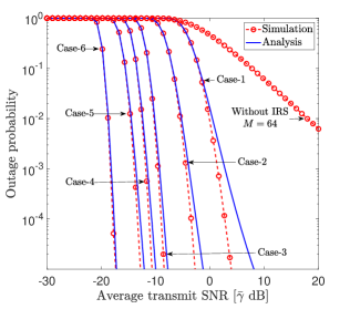
Figure 3: The outage probability for different $M$ and $N$ and $\gamma_{th}=0$ dB. The combinations of $M$ and $N$ for Case-1 to Case-6 are set to $\{M=36,N=16\}$, $\{M=36,N=32\}$, $\{M=16,N=64\}$, $\{M=36,N=64\}$, $\{M=64,N=64\}$, and $\{M=36,N=128\}$.

In Fig. 3, we plot the outage probability as a function of the average transmit SNR ($\bar{\gamma}$) for different combinations of distributed APs $(M)$ and reflective elements $(N)$ at the IRS. For comparison purposes, we also plot the outage probability for the APs-to-$D$ direct transmission (without using an IRS) for $M=64$ in the same figure. We use our closed-form derivation in (15) to plot the analytical outage probability approximations, and we plot the exact counterparts through Monte-Carlo simulation. The latter is used to verify the accuracy/tightness of our outage probability approximations. According to Fig. 3, the tightness of our outage analysis improves with as $M$ or/and $N$ increase. The reason for this is that large $M$ or/and $N$ improves the accuracy of CLT. Moreover, the outage probability can be reduced by either increasing $M$ or/and $N$. For example, at an average SNR of $-5\,$dB, the outage probability can be reduced by $99.9$% by doubling $N$ from $16$ (Case-1) to $32$ (Case-2) while keeping $M=36$. Moreover, by increasing $M,N$ from $\{M=36,N=32\}$ in Case-2 to $\{M=64,N=64\}$ in Case-4, the average SNR required to achieve an outage probability of $10^{-3}$ can be reduced by $155.6\%$ dB. From Fig. 3, we observe that the proposed IRS-aided cell-free set-up outperforms the APs-to-$D$ direct transmission. For instance, the set-up without IRS needs an average transmit SNR of $18$ dB to reach an outage probability of $10^{-2}$, which is about $177.6\%$ increase over the transmit SNR requirement for the Case-5 with the IRS-aided set-up for the same number of APs $(M=64)$. Thus, the co-existence of IRSs within a cell-free set-up can be beneficial in reducing the system outage probability.

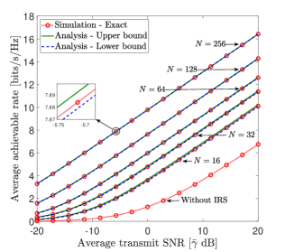
Figure 4: The average achievable rate for $N\in\{16,32,64,128,256\}$ and $M=64$.

In Fig. 4, we study the average achievable rate of the proposed system as a function of the average transmit SNR ($\bar{\gamma}$) for $N\in\{16,32,64,128,256\}$. We also compare the achievable rates of APs-to-$D$ direct transmission and the IRS-aided transmission. The upper and lower bounds for the achievable rates are plotted by using our analysis in (16) and (17), respectively. We again validate the accuracy of our analysis through Monte-Carlo simulations of the exact achievable rate. The tightness of our upper/lower rate bounds is clearly depicted in enlarged portion of Fig. 4. We observe that the rate gains can be achieved by increasing the number of reflective elements in the IRS. Fig. 4 also illustrates that an IRS can be embedded within a cell-free set-up to boost the achievable gains. For instance, an IRS with $N=16$ provides a rate gain of about $180$ % compared to the APs-to-$D$ transmission without an IRS at an average transmit SNR of $0$ dB.

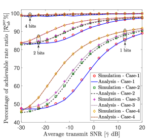
Figure 5: The impact of discrete phase-shifts with phase-shift quantization on the average achievable rate for different $M$ and $N$. The combinations of $M$ and $N$ for Case-1 to Case-4 are set to $\{M=36,N=32\}$, $\{M=64,N=32\}$, $\{M=36,N=64\}$, and $\{M=64,N=64\}$.

In Fig. 5, we investigate the impact of discrete phase-shifts and the number of quantization bits ($B$) by plotting the percentage rate ratio $(\mathcal{R}_{ub}^{per})$ against the average transmit SNR for different combinations of $M$ and $N$. The phase-shift quantization errors are uniformly distributed: $\mathcal{U}\left[-\pi/2^{B},\pi/2^{B}\right)$. The percentage rate ratio is defined as follows: $\mathcal{R}_{ub}^{per}=\hat{\mathcal{R}}_{ub}/\mathcal{R}_{ub}\times 100\%$, where $\hat{\mathcal{R}}_{ub}$ and $\mathcal{R}_{ub}$ are the upper bounds of the average achievable rate with and without phase-shift quantization errors given in (19) and (16), respectively. Monte-Carlo simulation curves are also generated to validate our analysis. Fig. 5 shows that the impact of phase-shift quantization errors vanishes when a higher $B$ is used. For instance, we can recover more than $98\%$ of the average rate when $4$ bit quantization is used at the IRS compared to the system with continuous phase-shift adjustments. As per Fig. 5, $\mathcal{R}_{ub}^{per}$ improves in the high SNR regime. For example, by varying $B$ as 1, 2, and 4 bits, the average rate can be recovered more than $90\%$, $98\%$, and almost $100\%$, respectively, at a transmit SNR of $20\,$dB. Fig. 5 shows that a higher number of $M,N$ is also beneficial for recovering the achievable rate in the moderate-to-large transmit SNR regime.

VII Conclusion

In this paper, the feasibility of adopting an IRS embedded within a cell-free set-up has been explored. The optimal received SNR through multiple distributed APs with an IRS-aided channel has been statistically characterized by deriving the tight PDF and CDF approximations. This probabilistic SNR analysis has been used to derive tight approximations/bounds for the outage probability and the average achievable rate in closed-form. The impairments of discrete phase-shifts with equalization errors have been explored. The accuracy of our performance analysis of the proposed system set-up has been verified by providing Monte-Carlo simulations. We observe from our numerical results that IRS-aided cell-free system set-ups may be used to reduce the outage probability and boost the achievable rates of next-generation wireless systems.

Appendix A The derivation of PDF of $\tilde{R}$ in (10)

By using the fact that $\lambda_{u}$ and $\tilde{Y}$ are independent random variables, we derive the PDF of $\tilde{R}$ as

$$f_{\tilde{R}}(x) = \int_{0}^{\infty}f_{u}(u)f_{\tilde{Y}}(x-u)du$$

$$\!\!\!\!\!\!\!\!\!\!\!\!\!\!\!\!\!\!\!=2a\rho\mathrm{e}^{-\frac{(x-\mu_{Y})^{2}}{2\sigma_{Y}^{2}}}\int_{0}^{\infty}u\mathrm{e}^{-au^{2}+bu}du$$

$$\!\!\!\!\!\!\!\!\!\!\!\!\!\!\!\!\!\!\!=2a\rho\mathrm{e}^{-\frac{(x-\mu_{Y})^{2}}{2\sigma_{Y}^{2}}}\mathrm{e}^{\frac{b^{2}}{4a}}\int_{0}^{\infty}u\mathrm{e}^{-a\left(u-\frac{b}{2a}\right)^{2}}du$$

$$\!\!\!\!\!\!\!\!\!\!\!\!\!\!\!\!\!\!\!\stackrel{{\scriptstyle(a)}}{{=}}2a\rho\mathrm{e}^{-\frac{(x-\mu_{Y})^{2}}{2\sigma_{Y}^{2}}}\mathrm{e}^{\frac{b^{2}}{4a}}\!\!\left(\underbrace{\int_{-b/2a}^{\infty}\!\!\!t\mathrm{e}^{-at^{2}}dt}_{I_{1}}+\frac{b}{2a}\underbrace{\int_{-b/2a}^{\infty}\!\!\!\mathrm{e}^{-at^{2}}dt}_{I_{2}}\right),$$

where $b=(x-\mu_{Y})/\sigma_{Y}^{2}$. The step $(a)$ is obtained by letting $t=u-b/2a$. Then, we can evaluate $I_{1}$ in (A) as

$$\!\!\!\!\!\!\!\!I_{1} = \int_{-b/2a}^{\infty}\!\!\!t\mathrm{e}^{-at^{2}}dt\stackrel{{\scriptstyle(b)}}{{=}}\left[-\mathrm{e}^{-at^{2}}/2a\right]_{-b/2a}^{\infty}=\mathrm{e}^{-b^{2}/2a},$$ (20)

where the step $(b)$ is computed by using [17, Eqn. 2.33.12]. Next, we evaluate $I_{2}$ as

$$I_{2} = \int_{-b/2a}^{\infty}\mathrm{e}^{-at^{2}}dt\stackrel{{\scriptstyle(c)}}{{=}}\left[\frac{\sqrt{\pi}\mathrm{erf}\left(\sqrt{a}t\right)}{2\sqrt{a}}\right]_{-b/2a}^{\infty}$$ (21)

$$= \frac{\sqrt{\pi}}{2\sqrt{a}}\left(1-\mathrm{erf}\left(\frac{-b}{2\sqrt{a}}\right)\right),$$

where the step $(c)$ is due to [17, Eqn. 2.33.16]. We substitute (20) and (21) into (A) to obtain the PDF of $\tilde{R}$ in (10).

Appendix B The derivation of CDF of $\tilde{R}$ in (13)

We substitute (10) into (13) to derive $I_{a}$ as

$$I_{a}\! = \!\sqrt{\pi}\rho\!\!\!\int_{x}^{\infty}\!\!\!\left(\!\frac{u-\mu_{Y}}{2\sigma_{Y}^{2}\sqrt{a}}\!\right)\!\mathrm{e}^{\!-\Delta\left(\!\frac{u-\mu_{Y}}{2\sigma_{Y}^{2}\sqrt{a}}\!\right)^{\!2}}\!\!\left(\!\mathrm{erf}\left(\frac{u-\mu_{Y}}{2\sigma_{Y}^{2}\sqrt{a}}\right)\!+\!1\!\right)du$$ (22)

$$\stackrel{{\scriptstyle(d)}}{{=}} \lambda\int_{d}^{\infty}t\mathrm{exp}\left(-\Delta t^{2}\right)\left(\mathrm{erf}\left(t\right)+1\right)dt$$

$$\stackrel{{\scriptstyle(e)}}{{=}} \lambda\left[\frac{-\mathrm{e}^{-\Delta t^{2}}(\mathrm{erf}\left(t\right)+1)}{2\Delta}\right]_{d}^{\infty}+\lambda\int_{d}^{\infty}\frac{\mathrm{e}^{-t^{2}(\Delta+1)}}{2\Delta}dt$$

$$\stackrel{{\scriptstyle(f)}}{{=}} \frac{\lambda\mathrm{e}^{-\Delta d}\left(\mathrm{erf}\left(d+1\right)\right)}{2\Delta}+\frac{\lambda\left(1-\mathrm{erf}\left(d\sqrt{\Delta+1}\right)\right)}{2\Delta\sqrt{\Delta+1}},$$

where $\lambda=2\sigma_{Y}^{2}\rho\sqrt{\pi a}$ and $d=(x-\mu_{Y})/(2\sigma_{Y}^{2}\sqrt{a})$. The step $(d)$ is obtained by through $t=(u-\mu_{Y})/2\sigma_{Y}^{2}\sqrt{a}$. The step $(e)$ is written by invoking part-by-part integration, while the step $(f)$ is due to [17, Eqn. 2.33.16]. Next, we compute $I_{b}$ as

$$I_{b} = \rho\int_{x}^{\infty}\mathrm{e}^{-\left(\frac{u-\mu_{Y}}{2\sigma_{Y}^{2}}\right)^{2}}du\stackrel{{\scriptstyle(g)}}{{=}}\sqrt{2\sigma_{Y}^{2}}\rho\int_{\sqrt{2\sigma_{Y}a}d}^{\infty}\mathrm{e}^{-t^{2}}dt$$ (23)

$$\stackrel{{\scriptstyle(h)}}{{=}} \sqrt{\frac{\pi\sigma_{Y}^{2}}{2}}\rho\left(1-\mathrm{erf}\left(\sqrt{2\sigma_{Y}a}d\right)\right),$$

where the step $(g)$ is due to a changing of dummy variable as $t=(u-\mu_{Y})/(2\sigma_{Y}^{2})$, and the step $(h)$ is resulted due to [17, Eqn. 2.33.16].

Appendix C The derivation of $\mathcal{R}_{lb}$ and $\mathcal{R}_{ub}$ in (17) and (16)

First, by invoking Jensen’s inequality, $\mathcal{R}_{lb}$ and $\mathcal{R}_{ub}$ can be defined as

$$\mathcal{R}_{lb} = \mathrm{log}_{2}\left(1+\left(\mathbb{E}\!\left[{1/\tilde{\gamma}^{*}}\right]\right)^{-1}\right),$$ (24a)

$$\mathcal{R}_{ub} = \mathrm{log}_{2}\left(1+\mathbb{E}\!\left[{\tilde{\gamma}^{*}}\right]\right).$$ (24b)

Then, we evaluate the expectation term in (24b) as

$$\mathbb{E}\!\left[{\tilde{\gamma}^{*}}\right] = \mathbb{E}\!\left[{\bar{\gamma}\tilde{R}^{2}}\right]=\bar{\gamma}\mathbb{E}\!\left[{(\lambda_{u}+\tilde{Y})^{2}}\right]$$ (25)

$$= \bar{\gamma}\sum_{n\in C_{2}}\!\!\binom{2}{n}\mathbb{E}\!\left[{\lambda_{u}^{(2-n)}}\right]\mathbb{E}\!\left[{\tilde{Y}^{n}}\right]$$

$$= \bar{\gamma}\left(\xi_{u}+\mu_{u}^{2}+\sigma_{Y}^{2}+\mu_{Y}^{2}+2\mu_{u}\mu_{Y}\right),$$

where $\mu_{u}=\sqrt{\pi\xi_{u}/2}$. Moreover, $\mu_{Y}$ and $\sigma_{Y}^{2}$ are given in (9a) and (9b), receptively. By substituting (25) into (24b), $\mathcal{R}_{ub}$ can be computed as (16). Next, we can write the expectation term in (24a) as

$$\mathbb{E}\!\left[{1/\tilde{\gamma}^{*}}\right]={1}/{\mathbb{E}\!\left[{\tilde{\gamma}^{*}}\right]}+{\mathbb{V}\mathrm{ar}\!\left[{\tilde{\gamma}^{*}}\right]}/{\left(\mathbb{E}\!\left[{\tilde{\gamma}^{*}}\right]\right)^{3}},$$ (26)

where $\mathbb{E}\!\left[{\tilde{\gamma}^{*}}\right]$ is defined in (25) and $\mathbb{V}\mathrm{ar}\!\left[{\tilde{\gamma}^{*}}\right]=\bar{\gamma}^{2}\mathbb{E}\!\left[{\tilde{R}^{4}}\right]-\left(\mathbb{E}\!\left[{\tilde{\gamma}^{*}}\right]\right)^{2}$. Then, we can compute $\mathbb{E}\!\left[{\tilde{R}^{4}}\right]$ as follows:

$$\!\!\!\!\!\!\!\!\mathbb{E}\!\left[{\tilde{R}^{4}}\right] = \mathbb{E}\!\left[{(\lambda_{u}+\tilde{Y})^{4}}\right]\!=\sum_{n\in C_{4}}\!\binom{4}{n}\mathbb{E}\!\left[{\lambda_{u}^{(4-n)}}\right]\mathbb{E}\!\left[{\tilde{Y}^{n}}\right],$$ (27)

where the $n$th moment of $\lambda_{u}^{n}$ is denoted by $\mathbb{E}\!\left[{\lambda_{u}^{n}}\right]$. We compute $\mathbb{E}\!\left[{\lambda_{u}^{n}}\right]$ as

$$\mathbb{E}\!\left[{\lambda_{u}^{n}}\right] = \int_{0}^{\infty}x^{n}f_{u}(x)dx=\int_{0}^{\infty}\frac{x^{n+1}}{\xi_{u}}\mathrm{exp}\left(-\frac{x^{2}}{2\xi_{u}}\right)dx$$ (28)

$$\stackrel{{\scriptstyle(i)}}{{=}} \left(2\xi_{u}\right)^{n/2}\Gamma\left(n/2+1\right),$$

where the step $(m)$ is evaluated from [17, Eqn. 2.33.10] and $\Gamma(t)=\int_{0}^{\infty}x^{t}\mathrm{e}^{-x}dx$ is the Gamma function [17, Eqn. 8.310.1]. Then, we evaluate $\mathbb{E}\!\left[{\tilde{Y}^{n}}\right]$ for $n\in C_{4}^{\prime}$ as

$$\mathbb{E}\!\left[{\tilde{Y}^{n}}\right] = \frac{\psi}{\sqrt{2\pi\sigma_{Y}^{2}}}\int_{0}^{\infty}y^{n}\mathrm{e}^{-\frac{(y-\mu_{Y})^{2}}{2\sigma_{Y}^{2}}}dy$$

$$\stackrel{{\scriptstyle(j)}}{{=}} \frac{\psi}{\sqrt{\pi}}\int_{{-\mu_{Y}}/{\sqrt{2\sigma_{Y}^{2}}}}^{\infty}\left(\sqrt{2\sigma_{Y}^{2}}t+\mu_{Y}\right)^{n}\mathrm{e}^{-t^{2}}dt$$

$$\stackrel{{\scriptstyle(k)}}{{=}} \!\frac{\psi}{2\sqrt{\pi}}\sum\limits_{i\in C_{n}}\!\!\binom{n}{i}\left({2\sigma_{Y}^{2}}\right)^{\frac{n-i}{2}}\mu_{Y}^{i}I\!\left(n\!-\!i,\frac{-\mu_{Y}}{2\sigma_{Y}^{2}}\right),$$

where the step $(j)$ is due to a changing of the dummy variable, the step $(k)$ is obtained by expanding $\left(\!\sqrt{2\sigma_{Y}^{2}}t\!+\!\mu_{Y}\!\right)^{\!\!n}\!$ based on $n\!$ value. Moreover, $\!I(\!\cdot,\cdot\!)\!$ is given as

$$\!\!\!\!\!\!\!\!\!I\!\left(m,t\right)\!=\!\begin{cases}(-1)^{m}\gamma\left(\frac{m+1}{2},t^{2}\right)+\Gamma\left(\frac{m+1}{2}\right),&\text{for}\,\,t\leq 0,\\ \Gamma\left(\frac{m+1}{2},t^{2}\right),&\text{otherwise},\end{cases}$$ (30)

where $\gamma(\lambda,x)=\int_{0}^{x}\mathrm{e}^{-t}t^{\lambda-1}dt$ is the lower incomplete Gamma function [17, Eqn. 8.350.1]. Finally, $\mathcal{R}_{lb}$ is derived as (17).

References

• [1] H. Q. Ngo et al., “Cell-Free Massive MIMO: Uniformly Great Service for Everyone,” in IEEE 16th Int. Workshop on Signal Process. Adv. in Wireless Commun. (SPAWC), June 2015, pp. 201–205.
• [2] ——, “Cell-Free Massive MIMO versus Small Cells,” IEEE Trans. Wireless Commun., vol. 16, no. 3, pp. 1834–1850, Mar. 2017.
• [3] M. D. Renzo et al., “Smart Radio Environments Empowered by Reconfigurable AI Meta-Surfaces: An idea whose time has come,” EURASIP J. Wireless Commun. Net., May 2019.
• [4] C. Liaskos et al., “A New Wireless Communication Paradigm through Software-Controlled Metasurfaces,” IEEE Commun. Mag., vol. 56, no. 9, pp. 162–169, 2018.
• [5] D. L. Galappaththige, D. Kudathanthirige, and G. Amarasuriya Aruma Baduge, “Performance Analysis of Distributed Intelligent Reflective Surface Aided Communications,” in IEEE Global Commun. Conf. (GLOBECOM), May 2020, pp. 1–6, (submitted).
• [6] H. Q. Ngo et al., “On the Total Energy Efficiency of Cell-Free Massive MIMO,” IEEE Trans. Green Commun. Netw., vol. 2, no. 1, pp. 25–39, 2018.
• [7] E. Nayebi et al., “Precoding and Power Optimization in Cell-Free Massive MIMO Systems,” IEEE Trans. Wireless Commun., vol. 16, no. 7, pp. 4445–4459, July 2017.
• [8] D. L. Galappaththige and G. Amarasuriya, “Cell-Free Massive MIMO with Underlay Spectrum-Sharing,” in IEEE Int. Conf. on Commun. (ICC), 2019, pp. 1–7.
• [9] Ö. Özdogan, E. Björnson, and E. G. Larsson, “Intelligent Reflecting Surfaces: Physics, Propagation, and Pathloss Modeling,” IEEE Wireless Commun. Lett., vol. 9, no. 5, pp. 581–585, 2020.
• [10] Q. Wu and R. Zhang, “Intelligent Reflecting Surface Enhanced Wireless Network via Joint Active and Passive Beamforming,” IEEE Trans. Wireless Commun., pp. 1–1, 2019.
• [11] Y. Han et al., “Large Intelligent Surface-Assisted Wireless Communication Exploiting Statistical CSI,” IEEE Trans. Veh. Technol., vol. 68, no. 8, pp. 8238–8242, Aug 2019.
• [12] J. Chen et al., “Intelligent Reflecting Surface: A Programmable Wireless Environment for Physical Layer Security,” IEEE Access, vol. 7, pp. 82 599–82 612, 2019.
• [13] S. Abeywickrama, R. Zhang, and C. Yuen, “Intelligent Reflecting Surface: Practical Phase Shift Model and Beamforming Optimization,” in IEEE Int. Conf. on Commun. (ICC), 2020, pp. 1–6.
• [14] Z. Ding and H. Vincent Poor, “A Simple Design of IRS-NOMA Transmission,” IEEE Commun. Lett., vol. 24, no. 5, pp. 1119–1123, 2020.
• [15] A. Papoulis and S. U. Pillai, Probability, Random Variables, and Stochastic Processes, 4th ed.   McGraw Hill, 2002.
• [16] Q. Wu and R. Zhang, “Towards Smart and Reconfigurable Environment: Intelligent Reflecting Surface Aided Wireless Network,” IEEE Commun. Mag., vol. 58, no. 1, pp. 106–112, 2020.
• [17] I. Gradshteyn and I. Ryzhik, Table of Integrals, Series, and Products, 7th ed.   Academic Press, 2007.
• [18] Q. Zhang et al., “Power Scaling of Uplink Massive MIMO Systems with Arbitrary-Rank Channel Means,” IEEE J. Sel. Areas Signal Process., vol. 8, no. 5, pp. 966–981, Oct. 2014.
• [19] S. Haykin and M. Moher, Communication Systems, 5th ed.   Wiley India Pvt. Limited, 2009.
• [20] T. L. Marzetta et al., Fundamentals of Massive MIMO.   Cambridge University Press, Cambridge, UK, 2016.