On the stability of satellites at unstable libration points of sun–planet–moon systems

Abstract

The five libration points of a sun–planet system are stable or unstable fixed positions at which satellites or asteroids can remain fixed relative to the two orbiting bodies. A moon orbiting around the planet causes a time-dependent perturbation on the system. Here, we address the sense in which invariant structure remains. We employ a transition state theory developed previously for periodically driven systems with a rank-1 saddle in the context of chemical reactions. We find that a satellite can be parked on a so-called time-periodic transition state trajectory—which is an orbit restricted to the vicinity of the libration point L2 for infinitely long time—and investigate the stability properties of that orbit.

1 Introduction

It is well known that a balance of forces between bodies in space can lead to stable or unstable fixed points in which a small body, such as a craft or satellite, experiences no net forces in a particular moving frame. The geostationary points arising from the cancellation of the gravitational force of the Earth and a satellite’s centrifugal force is a nice example. At this fixed point, the satellite remains forever fixed above a particular point on the Earth’s surface as both rotate in tandem. Five fixed points are known to exist in the two-body Sun–Earth system and are called the libration or Lagrange points L1 to L5 [1, 2], as schematically illustrated in Fig. 1. The three collinear libration points L1 to L3 are unstable because small deviations from the exact position increase with time leading to the decay of the satellite away from them. However, the other two triangular libration points L4 and L5 can be stable because of the effects of the Coriolis force, if the ratio of the masses of the sun and planet is sufficiently large [3, 1].

The dynamics of planetary systems becomes much more complicated as soon as a third primary such as a moon is considered [4, 5, 6, 7, 8]. In this case, the stability and position of the libration points in the rotating frame are influenced by the Moon’s gravitational force. That is, the Moon’s rotation around the Earth causes a time-dependent periodic driving of the satellite and it is a non-trivial question whether or not the satellite can still stay forever in the local vicinity of a libration point. In this paper, we address this question with respect to the libration point L2. We characterize the dynamics and stability of a satellite near this point in a generic sun–planet system while explicitly considering the effects from the moon’s rotation. The dynamics near the unstable libration points is determined by a rank-1 saddle of the potential. To investigate the dynamics close to the saddle we resort to the use of transition state theory (TST) [9, 10, 11, 12, 13, 14, 15]. In chemical reactions without driving, the precise determination of a dividing surface (DS) separating reactants and products is key to determining rate constants. TST rates are given by the particle flux through that surface [16, 17, 18, 19, 20, 21, 22, 23, 24, 25, 26, 27]. It has been applied in various fields of physics and chemistry, including, e. g., atomic physics [28], solid state physics [29], cluster formation [30, 31], diffusion dynamics [32, 33], and cosmology [34], to name a few. A version of TST has also been implemented to describe the escape of satellites from planetary neighborhoods in celestial mechanics [35, 36]. Here, we use recent advances in TST for driven chemical reactions [37, 38, 39, 40] to generalize such a treatment to include the effects of a moon on the escape of a satellite from L2.

Figure 1: Schematic of a generic solar system in the BCR4BP. A planet and its moon are on circular orbits about their mutual barycenter. This planet–moon barycenter and the sun both move around the total center of mass. Other bodies in this system—e. g., satellites or asteroids—are assumed to have negligible mass. All orbits are coplanar. Without the moon, the system is known to give rise to the five libration points, marked L1 to L5, associated with the stability of additional objects such as a satellite or asteroid. The unstable point L2 is the focus of this work. In the special case of our Solar System, these bodies refer to the Sun, the Earth and the Moon. Here, we consider a broader range of cases and list the corresponding parameters in Table 1.

The paper is organized as follows: In Sec. 2, we introduce the formulation of the bicircular restricted four-body problem (BCR4BP) [4, 5, 6, 7] used throughout this paper. In addition to specifying the system, we also derive the corresponding equations of motion and give a short review of the libration points. In Sec. 3, we present a brief introduction to TST and the numerical methods used for the analysis of the phase space structure, the determination of the periodic libration point orbit, and the stability analysis of that orbit. Finally, we show in Sec. 4 that the fixed point associated with the L2 evolves into a periodic libration point orbit when the moon’s effects on the system are explicitly included. Our central finding is that the decay rates for satellites on this orbit can be obtained using a transition state theory framework, and in so doing, revealing the geometric structure of its dynamics. Using the calculated decay rates for satellites on this orbit, the TST approach allows for the determination of the effort needed to actively stabilize satellites near L2 as a time-dependent function of the moon’s position.

2 The model solar system

We focus on planetary systems with three primary bodies to illustrate the use of TST in celestial mechanics. Unfortunately, there does not exist a general closed-form solution for such three-body problems [41] that would provide a rigorous benchmark. We therefore base our calculations on the well-known BCR4BP which models three primaries on fixed circular orbits in the same two-dimensional plane [4, 5, 6, 7]. The two lighter primaries—referred to as planet and moon—orbit their mutual barycenter in an inner nested two-body problem. In turn, this planet–moon barycenter and the heaviest primary—the sun—orbit the total system’s center of mass as shown in Fig. 1 Although this center of mass is itself a barycenter for the whole system, we will avoid referring it as such through the text to avoid confusion. In the outer nested two-body problem, the planet and moon are treated as a single body located at their barycenter. The dynamics of the probe body (for example an asteroid or satellite) is governed by the primaries’ gravitational forces. Its mass is assumed to be so small that its gravitational force on other bodies can be neglected.

2.1 Libration points in the sun–planet system

A system consisting of two bodies interacting via gravitational forces—in our case a sun and a planet—features five points where the gravitational forces and the centrifugal force on a probe mass nullify each other. These equilibrium points are called the libration or Lagrange points L1 to L5. Figure 1 schematically shows the position of L1 to L5 relative to the celestial bodies. The libration points rotate with the same frequency as the primaries, and therefore the probe mass’ position relative to the bodies is constant. This makes them very interesting for space exploration and research [42, 43, 44]. Adding a lighter third primary—i. e., a moon orbiting the planet—causes a time-dependent perturbation of the libration points. See Sec. 4.1 for a more detailed discussion.

The libration points differ by their stability properties. The potentials near L1 to L3 are rank-1 saddles with one unstable degree of freedom (DoF) in the radial direction and one stable DoF perpendicular to the radial direction. Trajectories near L1 to L3 are therefore unstable. The libration points L4 and L5 show as rank-2 saddles with two unstable directions. Contrary to first intuition, however, trajectories near L4 and L5 are Lyapunov stable for sufficiently large sun–planet mass ratios [3, 1] because of the contributions from the velocity-dependent Coriolis force [3, 45]. However, trajectories near the collinear libration points L1 to L3 are not stabilized in similar fashion despite the effects from the Coriolis force.

In this paper we will focus on the stability of satellites near L2 and the influence of a moon thereupon. In our Solar System, L2 is especially interesting for astrophysics since it is located far enough from Sun, Earth, and Moon to minimize noise but still close enough to Earth for communication. It has been the target of multiple past and present space missions, e. g., the Wilkinson Microwave Anisotropy Probe [46], the James Webb Space Telescope [47], the Herschel mission [48], and the Planck spacecraft [49]. In addition, it features a rank-1 saddle which can be readily described using the framework of TST as summarized in Sec. 3.

2.2 Parameters and model variants

Table 1: Summary of the configuration parameters and derived values used in the strong-driving and Solar System models considered here. We use dimensionless units derived from a synodic coordinate system with respect to the sun and the planet–moon barycenter. The sun–barycenter distance, sun–barycenter angular frequency, and total mass of all primaries are used as units for length, frequency, and mass, respectively. The satellite is assumed to be an infinitesimal mass point. Its mass gets canceled from the equations of motion, and there is no need to specify it. See Sec. 2.3 for further details.

description	symbol	strong-driving model	Solar System model
planet–moon distance	$a$	$0.1$	$2.570\text{\times}{10}^{-3}$
primary mass parameter	$\mu$	$0.1$	$3.040\text{\times}{10}^{-6}$
secondary mass parameter	$\tilde{\mu}$	$0.1$	$1.215\text{\times}{10}^{-2}$
sun mass	$M_{\mathrm{S}}=1-\mu$	$0.9$	$0.999\,997$
barycenter mass	$M_{\mathrm{B}}=\mu$	$0.1$	$3.040\text{\times}{10}^{-6}$
planet mass	$M_{\mathrm{P}}=\mu(1-\tilde{\mu})$	$0.09$	$3.003\text{\times}{10}^{-6}$
moon mass	$M_{\mathrm{M}}=\mu\tilde{\mu}$	$0.01$	$3.695\text{\times}{10}^{-8}$
synodic moon frequency	$\omega=\sqrt{\mu/a^{3}}-1$	$9$	$12.387$

We use dimensionless units derived from a synodic reference frame with respect to the sun and the planet–moon barycenter. The sun–barycenter distance, the sun–barycenter angular frequency, and the total mass of all primaries act as units for length, frequency (inverse time), and mass, respectively. The gravitational constant follows as $G=1$. In this coordinate system, the total center of mass is at the origin with the sun and the barycenter located at $(-\mu,0)^{\mathsf{T}}$ and $(1-\mu,0)^{\mathsf{T}}$, respectively. The primary mass parameter $\mu$ is defined as the barycenter mass (i. e., sum of planet and moon mass) in units of the system’s total mass. The planet and moon orbit with distance $a$ and angular frequency $\omega$ around the barycenter. The secondary mass parameter $\tilde{\mu}$ is defined analogously as the moon mass divided by the barycenter mass, cf. Table 1.

The BCR4BP is only an approximation to the real dynamics. We can recover strict Newtonian motion of the primaries by removing the moon ($\tilde{\mu}=0$). This limiting case is equivalent to the circular restricted three-body problem (CR3BP) and will be referred to as the time-invariant or static system because the resulting potential is time-independent in the synodic frame. In contrast, models with $\tilde{\mu}\neq 0$ will be called driven as the moon perturbs the potential even in the synodic frame.

In this work, we consider two parameterizations of the BCR4BP listed in Table 1:

1. In the strong-driving model, the mass parameters are taken as $\mu=\tilde{\mu}=$0.1$$ and the planet–moon distance as $a=$0.1$$. The chosen values lead to a stronger perturbation of L2 and allow for easier visualization. This parameter set is characteristic of the more extreme mass ratios that have been observed in extrasolar systems. An example is the brown dwarf 2M1207A and its companion planet 2M1207b [50] located in the constellation Centaurus with masses around $60\text{\,}\mathrm{\mathit{M}_{J}}$ and $5\text{\,}\mathrm{\mathit{M}_{J}}$ ($\mathrm{\mathit{M}_{J}}$ being the Jovian mass), respectively. Therein the mass parameter is $\mu\approx$0.077$$, and is comparable to the value in our parameter set. The corresponding effective potential is shown in Fig. 2.

2. In our Solar System, the masses of the Sun, the Earth, the Moon, and the relative distances between them are well known. It provides a comparison to the strong-driving model, and demonstrates the applicability of our methods.

2.3 Potential and equations of motion

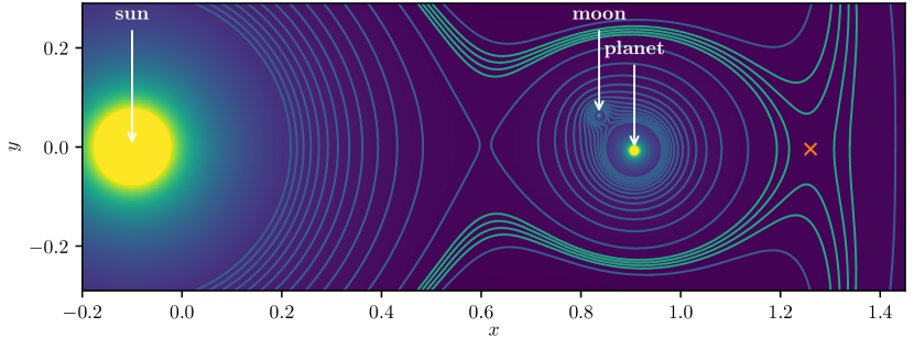
Figure 2: Effective potential $V_{\mathrm{eff}}(x,y,t)$ according to Eq. (6) at $t=3T/8$ for the strong-driving model. The color map is capped at $V_{\mathrm{eff}}=$-12$$ since the potential is divergent at the positions of the system’s sun, planet, and moon (filled yellow circles). A cross indicates the dynamical position of the saddle point near L2. We caution the reader that this point does not necessarily correspond to an equilibrium position due to the potential’s time dependence. More equipotential lines are shown near L2 to elucidate the saddle structure.

The bodies have normalized masses

$$M_{\mathrm{S}}=1-\mu,\quad M_{\mathrm{B}}=\mu,\quad M_{\mathrm{P}}=\mu(1-\tilde{\mu}),\quad\mbox{and\quad}M_{\mathrm{M}}=\mu\tilde{\mu}$$ (1)

where

$$0\leq\mu,\tilde{\mu}\leq 1\mbox{\quad and\quad}M_{\mathrm{S}}+M_{\mathrm{B}}=M_{\mathrm{S}}+M_{\mathrm{P}}+M_{\mathrm{M}}=1\,\text{.}$$ (2)

They are located at positions

$$\bm{R}_{\mathrm{S}}=-\mu\hat{{\bf\it e}}_{x},\quad\bm{R}_{\mathrm{B}}=(1-\mu)\hat{{\bf\it e}}_{x},\quad\bm{R}_{\mathrm{P}}=\bm{R}_{\mathrm{B}}-a\tilde{\mu}\hat{{\bf\it e}}_{\theta},\quad\mbox{and\quad}\bm{R}_{\mathrm{M}}=\bm{R}_{\mathrm{B}}+a(1-\tilde{\mu})\hat{{\bf\it e}}_{\theta}$$ (3)

where

$$\hat{{\bf\it e}}_{\theta}=\matrixquantity(\cos\theta\\ \sin\theta)\mbox{\quad with\quad}\theta=\omega t\mbox{\quad and\quad}\omega=\sqrt{\mu/a^{3}}-1$$ (4)

in the synodic coordinate system. Using the position of the satellite $\bm{r}$ relative to the primaries

$$\bm{r}_{j}=\bm{r}-\bm{R}_{j}\mbox{\quad for\quad}j\in\{\mathrm{S},\mathrm{P},\mathrm{M}\}$$ (5)

the effective potential can be written as

$$-V_{\mathrm{eff}}=\Omega=\frac{r^{2}}{2}+\frac{1-\mu}{r_{\mathrm{S}}}+\frac{\mu(1-\tilde{\mu})}{r_{\mathrm{P}}}+\frac{\mu\tilde{\mu}}{r_{\mathrm{M}}}\,\text{.}$$ (6)

This potential for the parameters of the strong-driving model is shown in Fig. 2.

The equations of motion for $\bm{r}=(x,y)^{\mathsf{T}}$ can be derived from the effective potential as

$$\dot{p}_{x}=\ddot{x}-2\dot{y}=\partialderivative{\Omega}{x}\mbox{\quad and\quad}\dot{p}_{y}=\ddot{y}+2\dot{x}=\partialderivative{\Omega}{y}$$ (7)

where

$$\partialderivative{\Omega}{j}=j-\sum_{k\in\{\mathrm{S},\mathrm{P},\mathrm{M}\}}\frac{M_{k}}{r_{k}^{3}}\bm{r}_{k}\dotproduct\hat{{\bf\it e}}_{j}\mbox{\quad for\quad}j\in\{x,y\}\,\text{.}$$ (8)

The terms $-2\dot{y}$ and $+2\dot{x}$ in Eqs. (7) account for the Coriolis force.

3 Transition state theory

The sun–planet–moon systems—described by the effective potential (6)—features a rank-1 saddle point at L2, as shown in Fig. 2, which can act as bottleneck of the dynamics. This makes it a prime candidate for the application of TST models. (See, e.g., Refs. [35, 51, 36].) In typical scenarios for a chemical reaction, a rank-1 saddle point separates reactants from products, and can be used to characterize the flux and associated reaction rate. In the planetary system, reactants roughly correspond to satellites or asteroids inside the planet’s Hill sphere [2, 51], and the reaction corresponds to the escape from this sphere, or vice versa. The unstable states between reactants and products form the transition state (TS). Thus geometrically, the TS is a boundary (or DS) between the reactant and product regions which in the current context corresponds to the DS between incoming or outgoing directions of the satellite. In planetary systems, this includes all libration point orbits. The reaction coordinate $x$ (in the rotating frame) describes the saddle’s unstable direction and indicates the progress of the reaction, see Fig. 3(a). The stable directions are referred to as orthogonal modes $\bm{y}$.

3.1 Geometry of the transition state

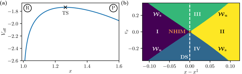
Figure 3: Position space and phase space at $t_{0}=0$ near L2 of the strong-driving model defined in Table 1. (a) A one-dimensional cut of the effective potential $V_{\mathrm{eff}}(x,y=0)$ along $x$. Reactants (R) and Products (P) are separated by a saddle in $V_{\mathrm{eff}}$. (b) The corresponding cut of the structures in phase space $(x,y=0,v_{x},v_{y}=0)$ near the NHIM at $x^{\ddagger}(y=0,v_{y}=0)\approx$1.260\,30$$. The NHIM’s stable $\mathcal{W}_{\mathrm{s}}$ and unstable $\mathcal{W}_{\mathrm{u}}$ manifolds divide the phase space into four nonreactive (I and II) and reactive (III and IV) regions. The NHIM acts as an anchor for the DS.

While it is straightforward to define a DS for a static 1-DoF system, differentiating between reactants and products in higher-dimensional or driven systems requires a more sophisticated mathematical framework though the analogy to the sun–planet–moon system remains.

We start by looking at the phase space near the saddle point. Depending on where they come from when propagating backward in time and where they go to when propagating forward in time, initial conditions of trajectories can be classified as either (I) nonreactive reactants, (II) nonreactive products, (III) reactive reactants, or (IV) reactive products. In the context of libration points, the terms reactive and nonreactive can be reframed as transit and nontransit orbits, respectively [52, 6]. The four regions are separated by critical trajectories forming the stable and unstable manifolds, as shown in Fig. 3(b). Trajectories on the stable manifold $\mathcal{W}_{\mathrm{s}}$ are bound to the saddle’s vicinity for $t\to\infty$ while trajectories on the unstable manifold $\mathcal{W}_{\mathrm{u}}$ are bound for $t\to-\infty$. They play an important role in the determination of efficient transfer orbits for spacecrafts [52, 6, 53, 54, 7]. These manifolds are associated with the normally hyperbolic invariant manifold (NHIM) [55, 56, 57, 5, 58, 59], where trajectories are bound both forward and backward in time. The NHIM is located at the intersection of the stable and unstable manifolds’ closures. It is this object that trajectories on $\mathcal{W}_{\mathrm{s}}$ and $\mathcal{W}_{\mathrm{u}}$ converge towards for $t\to+\infty$ and $-\infty$, respectively.

The NHIM plays an important role in determining whether a given state is considered a reactant or product—viz. pre– or post– escape in the present celestial models [35, 51, 36]. As shown in previous work [60, 61, 62, 63, 37], a (locally) recrossing-free codimension-$1$ DS can often be constructed by attaching it to the codimension-$2$ NHIM. In the simplest case, this is done by extending the NHIM in $v_{x}$ direction, as shown in Fig. 3(b). The DS then divides the phase space into a reactant and a product half. This construction even works when the saddle is subjected to time-dependent driving. In this case, the NHIM detaches from the position of the saddle point.

The NHIM can be obtained using several perturbative [24, 31] and direct [64, 15, 62] methods, but we have found that the binary contraction method (BCM) introduced in Ref. [65] is effective and efficient for systems such as the one addressed here. The algorithm in the BCM is initialized by defining a quadrangle with each of its corners lying exclusively within one of the four regions shown in Fig. 3(b). In each iterative step, we first determine an edge’s midpoint. Then, the adjacent corner corresponding to the same region as that midpoint is moved to the midpoint’s position. By repeating this interleaved bisection procedure in turn for all edges, the quadrangle successively contracts and converges towards the NHIM.

3.2 Instantaneous decay rates

The stability of the TS near threshold energy can be quantified via the decay of trajectories near the NHIM. This is equivalent to the rate at which an ensemble of reactants—i. e., asteroids or satellites on one side of the DS—moves through the DS. The decay of this reactant population is exponentially fast because of the hyperbolic nature of the NHIM. We can therefore define an instantaneous decay rate $k(t)$ via the differential equation [66, 38, 40, 67]

$$k(t)=-\frac{\dot{N}(t)}{N(t)}\,\text{,}$$ (9)

where $N(t)$ is the time-dependent size of the reactant population. Compared to other measures of instability, instantaneous decay rates have the advantage that they can be evaluated for a specific point in time. Floquet multipliers and Lyapunov exponents, for instance, only yield average values for a whole period and long-term limits, respectively.

The ensemble method [38, 40, 67] can be used to obtain the instantaneous decay rate of a reactant population close to the NHIM, which anchors the TS. A homogeneous and linear ensemble of $N$ reactive trajectories is initialized on the reactant side of the full phase space. Specifically, they are placed on an $(x,p_{x})$-cross sectional surface at a small distance $\delta x$ from a given position $(x^{\ddagger}(t),\bm{y}^{\ddagger}(t),p_{x}^{\ddagger}(t),\bm{p}_{y}^{\ddagger}(t))^{\mathsf{T}}$ of an arbitrarily chosen trajectory on the NHIM (see upper bullets in Fig. 4). After propagating this ensemble for a time $\delta t$, a subdomain will have pierced the DS and entered the product side (diamonds in Fig. 4) while the remainder will still be located on the reactant side (lower bullets in Fig. 4). As the DS is non-recrossing, the resulting decrease of the reactant population in a close neighborhood of the NHIM (cf. Eq. (9)) is associated with a decay rate

$$k_{\mathrm{e}}(\bm{y},\bm{p}_{y},t)=-\derivative{t}\ln[N(\bm{y},\bm{p}_{y},t)]\,\text{.}$$ (10)

It is referred to as the instantaneous ensemble rate to emphasize that it is obtained by propagating an ensemble of reactive trajectories according to the equations of motion. In doing so, the DS is computed individually for each trajectory of the ensemble and each time step.

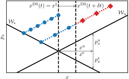
Figure 4: Schematic of instantaneous rate calculations. Initially, an equidistant ensemble connecting $\mathcal{W}_{\mathrm{s}}$ on the reactant side with the DS parallel to $\mathcal{W}_{\mathrm{u}}$ is generated. Upon time propagation, parts of the ensemble react through the DS. The resulting ensemble is still equidistant, parallel to $\mathcal{W}_{\mathrm{u}}$, and connected to $\mathcal{W}_{\mathrm{s}}$.

The ensemble can be propagated not just for a small time step $\delta t$ but for longer times when computing the time-dependent ensemble rate according to Eq. (10). As the reactant population decreases exponentially when propagating the ensemble, a new ensemble can be initialized close to the corresponding point of the respective trajectory on the NHIM after an appropriately chosen propagation time. Such technical details are discussed in Ref. [38]. Although the implementation of the ensemble method is straightforward, it can be numerically expensive because the ensemble consists of many trajectories and the DS is obtained individually for each reactive trajectory using the BCM [65].

The accuracy of the ensemble method decay rates decreases with time because of the reduction of the density of reactants. However, the inaccuracy can be reduced at the cost of larger computational expense by starting bigger ensembles or starting the ensembles staggered. Alternatively, we can avoid most of the expensive particle propagation of the ensemble method by leveraging the geometry of the stable and unstable manifolds to effectively describe the linearized dynamics near the NHIM (see A). The resulting local manifold analysis (LMA) method [38] can thus be seen as an extension to the ensemble method with the difference that the time when trajectories have reached the DS can now be determined analytically through the linearization thereby avoiding a costly numerical integration. As a result, the computational effort required to calculate instantaneous decay rates is significantly reduced while numerical precision is simultaneously enhanced. For reference, calculating $k$ for a single point on the NHIM (optimized for maximal precision, including two BCM calls) took about $15\text{\,}\mathrm{s}$ on an Intel i5-3470 CPU at $3.2\text{\,}\mathrm{GHz}$ for the system considered here. Lower-precision results can be obtained significantly faster. Additionally, these calculations can be trivially parallelized for entire trajectories. Compared to previous publications, the LMA method was extended to account for velocity-dependent forces (e. g. the Coriolis force) that arise from the rotating bodies in the sun–planet–moon system. The details can be found in B.

3.3 Floquet rate method

The LMA is significantly cheaper to evaluate than a full ensemble propagation. The numerical effort required, however, can still render it impractical when analyzing a large number of trajectories. When only time-averaged rate constants of periodic orbits are sought-after, a more tractable approach is provided by the Floquet rate method introduced in Ref. [68]. It determines the rate constant

$$\bar{k}_{\mathrm{F}}=\mu_{\mathrm{u}}-\mu_{\mathrm{s}}$$ (11)

for an orbit on the NHIM with period $T$ as the difference between the Floquet exponents

$$\mu_{\mathrm{u,s}}=\frac{1}{T}\ln|m_{\mathrm{u,s}}|\,\text{.}$$ (12)

The Floquet multipliers $m_{\mathrm{u,s}}$ are the eigenvalues of the monodromy matrix, i. e., of the fundamental matrix $\bm{\sigma}(t;t_{0})$ evaluated at time $t=t_{0}+T$. The fundamental matrix is calculated by solving the differential equation

$$\dot{\bm{\sigma}}(t;t_{0})=\bm{J}(t)\bm{\sigma}(t;t_{0})\mbox{\quad with\quad}\bm{\sigma}(t_{0};t_{0})=\bm{1}_{2d}$$ (13)

and where $\bm{J}$ is the Jacobian of the equations of motion (cf. A), $d$ is the number of DoF, and $\bm{1}_{2d}$ is the $(2d\times 2d)$-dimensional identity matrix. Evaluating a full trajectory with this method takes on the order of $10\text{\,}\mathrm{ms}$ on an Intel i5-3470 CPU at $3.2\text{\,}\mathrm{GHz}$.

4 Results and discussion

In this section we mainly focus on the dynamics on the NHIM and the rate of instability that can be derived from it. Since the NHIM is a hyperbolic subspace, trajectories need to be stabilized to not deviate numerically. This is achieved by periodically projecting satellites back using the BCM (cf. Sec. 3.1). When this is done frequently enough, errors introduced by this projection are negligible.

4.1 Dynamics on the NHIM

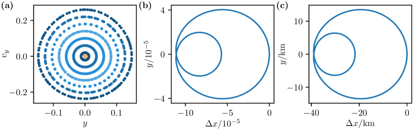
Figure 5: (a) Stroboscopic PSOS of the strong-driving model with $7$ trajectories propagated over $100$ periods on the NHIM starting at initial time $t_{0}=$0$$ (blue circles). The system exhibits regular dynamics as shown by the concentric tori. In its center, a fixed point (orange cross) reveals the existence of a periodic orbit with the system’s period $T$. (b) The periodic orbit from (a) in position space. Positions $\Delta x$ are relative to the position $\bm{\gamma}(t_{0})\approx($1.260\,47$,$0$,$0$,$-7.6\text{\times}{10}^{-4}$)^{\mathsf{T}}$. (c) The analogous periodic orbit for the Solar System model.

The dynamics on the NHIM of the periodically driven model system takes place in an effectively two-dimensional phase space. An established method for the visualization of such systems is the stroboscopic map, a special case of the Poincaré surface of section (PSOS). We propagate satellites on the NHIM. Instead of recording the whole trajectory, however, we only record one point every period $T=2\pi/\omega$. Trajectories with period $T$ therefore manifest as fixed points in the PSOS.

Figure 5(a) shows the stroboscopic PSOS of the driven model system’s NHIM around L2. One can see concentric toroidal structures, suggesting regular behavior. Trajectories associated with these tori are mostly quasi-periodic. The tori surround an elliptic fixed point, whose associated periodic trajectory is shown in Fig. 5(b). This orbit has the same period as the moon’s synodic orbit. It can be seen as the generalization of the static L2 point from the CR3BP. Similar observations have been made before, e. g., in Ref. [5] for the triangular libration points. In the following, we will therefore refer to this trajectory as the L2 orbit. It has been shown previously [38, 40] that elliptic fixed points are typically associated with extrema in the averaged decay rate. Consequently, there exists a region around the fixed points with similar decay rates. Thus to characterize the escape of satellites in the present time-dependent system, we must first determine the L2 orbit and then calculate the decay from it as we do in the following subsection.

The analogous L2 orbit for the Solar System model is shown in Fig. 5(c). It exhibits the same structure as the strong-driving model, but with a much lower orbit diameter of $\Delta x\approx$2.6\text{\times}{10}^{-7}$$ simulation units.

4.2 Decay rates

At this point, we are able to analyze the stability of satellites close to the L2 in our system. For this purpose, we calculate decay rates of satellites following the L2 orbit with the three methods presented in Secs. 3.2 and 3.3. The ensemble method has been configured to propagate $32$ ensembles of $1024$ satellites each. The ensembles are initialized at a maximum distance of $\delta x=$2\text{\times}{10}^{-4}$$ from the L2 orbit. We use $\delta x=${10}^{-5}$$ when determining the slopes of the stable and unstable manifolds for the LMA.

The instability of the L2 orbit as determined by the decay rate is shown in Fig. 6. Numerical values for the averaged rate constants are summarized in Table 2. As can be seen, all methods are in excellent agreement. The relative deviation between mean rates in the driven system is

$$\absolutevalue{\frac{\bar{k}_{a}-\bar{k}_{b}}{\bar{k}_{b}}}<${10}^{-5}$\mbox{\quad where\quad}\bar{k}_{a},\bar{k}_{b}\in\left\{\bar{k}_{\mathrm{e}},\bar{k}_{\mathrm{m}},\bar{k}_{\mathrm{F}}\right\}\,\text{.}$$ (14)

This confirms the accuracy of the results since all three methods have vastly different numerical implementations.

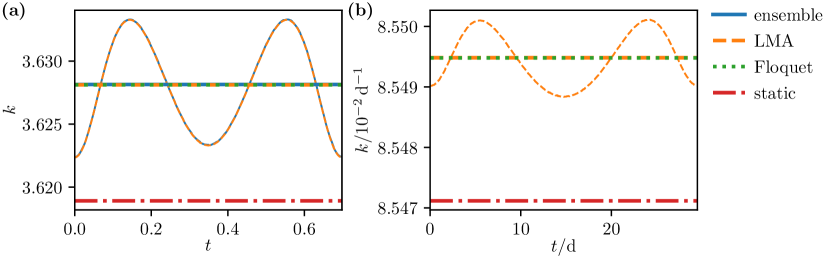
Figure 6: Instantaneous rates $k$ as a function of time $t$ for the periodic trajectories in Fig. 5. Results for the strong-driving model are shown in panel (a) while the Solar System model is represented in panel (b). The instantaneous rate $k(t)$ (thin lines) and time average $\bar{k}$ (thick lines) are shown for the ensemble method $k_{\mathrm{e}}$ [solid, panel (a) only] and the LMA method $k_{\mathrm{m}}$ (dashed). They are in agreement with each other, and with the corresponding Floquet rate $\bar{k}_{\mathrm{F}}$ (thick dotted). For comparison, $\bar{k}_{\mathrm{F}}$ of the corresponding static systems, in which the moon is effectively removed by setting $\tilde{\mu}=0$, is shown with a dash-dotted line.

Table 2: Numerical values for the averaged rate constants shown in Fig. 6 for the corresponding L2 orbits shown in Figs. 5(b) and  5(c). The ensemble propagation rate for the Solar System model is not listed because it was not calculated so as to avoid the unnecessary computational expense.

description	symbol	strong-driving model	Solar System model [${\mathrm{d}}^{-1}$]
ensemble propagation	$\bar{k}_{\mathrm{e}}$	$3.628\,145$
local manifold analysis	$\bar{k}_{\mathrm{m}}$	$3.628\,115$	$8.549\,482\text{\times}{10}^{-2}$
Floquet stability analysis	$\bar{k}_{\mathrm{F}}$	$3.628\,116$	$8.549\,479\text{\times}{10}^{-2}$
static system ($\tilde{\mu}=0$)	$\bar{k}_{\mathrm{F}}$	$3.618\,910$	$8.547\,117\text{\times}{10}^{-2}$

We show results for both the L2 orbit of the driven system (with moon, $\tilde{\mu}>0$) and the L2 point of the static system (without moon, $\tilde{\mu}=0$) as defined in Sec. 2. In the latter case, we restrict our analysis to the Floquet rate method as the instantaneous rate in static systems is constant in time and does not yield additional information.

In the comparison to the static system ($\tilde{\mu}=0$) in Fig. 6(a), we find a $+0.3\text{\,}\mathrm{\char 37\relax}$ increase in the average decay rate of the driven system. That is, the moon generally destabilizes satellites close to the L2 orbit. During one period of the orbit, L2 is most stable around $t\bmod T\in\{0,T/2\}$, i. e., when the planet, moon and L2 are collinear. At these points in time, either the planet or the moon are at their point of minimal distance from L2, therefore exerting the strongest forces on satellites near L2. Stronger forces push the position of L2 further out. This is consistent with the course of the L2 orbit shown in Fig. 5(b), which reaches maxima in $x$ around $t\bmod T\in\{0,T/2\}$. The lower decay rates entail that satellites near but not on the NHIM depart slower from L2. Consequently, fewer course corrections are needed around these points in time.

The limiting case that merges the planet and moon into a single effective body can be achieved by setting $\tilde{\mu}=0$. This keeps the system’s total mass fixed and only changes the mass distribution between planet and moon. Alternatively, we can consider the case in which the sun–planet mass ratio $M_{\mathrm{S}}/M_{\mathrm{P}}$ is kept fixed by setting the mass parameter $\mu=$0.09$/$0.99$$. The resulting Floquet rate constant now reads $\bar{k}_{\mathrm{F}}\approx$3.665$$. In this case, the addition of a moon leads to a $-1.0\text{\,}\mathrm{\char 37\relax}$ decrease of the rate constant. Hence, the effect of the moon is similar to a static system with an increased planet mass. The resulting stronger forces being exerted on satellites push the L2 further out.

The calculations of the LMA rates and the Floquet rate constants were also performed for the Solar System model. The results, shown in Fig. 6(b), are qualitatively identical to those of the strong-driving model discussed above. The decay rate oscillations and the relative deviation between the static and the driven systems, however, are quantitatively smaller by an order of magnitude.

5 Conclusion and outlook

In this work, we have demonstrated that the methods from TST can be used to analyze the dynamics of satellites in planetary systems. Specifically, we analyzed a generic solar system model based on the BCR4BP. We showed how TST approaches can be used to elucidate the dynamics of satellites in the vicinity of the sun–planet libration point L2, and to determine the extent to which they are influenced by the presence of a moon.

Two sets of parameters were investigated. The first was chosen to show a more significant effect while still resembling real, experimentally observed extrasolar systems. Although there has not yet been a confirmed moon observed around exoplanets [69, 70], this work provides a basis for describing L2 for such systems in the future. For comparison, the calculations were repeated for parameters resembling our Solar System. We found that a moon has a destabilizing effect on satellites near L2 when compared to a system in which planet and moon are merged into a single body. Interestingly, the decay rate when the planet and moon are collinear with the sun and L2 is lower than the average rate, suggesting a reduced need for stabilization by a satellite at that instant. To obtain these results, the LMA method has been generalized to address velocity-dependent forces, such as the Coriolis force. (See B for details.)

We found that TST can be used to describe not only driven chemical reactions, but also driven astrophysical systems. The rate of instability calculated in this paper describes how fast trajectories depart from the invariant manifold at L2 when they are not located exactly on said manifold. In principle, this rate therefore relates to the amount of fuel needed to actively stabilize a satellite on a specific orbit. When using system parameters typical of our Solar System, the methods presented here could be used to optimize the orbits of satellites with respect to fuel consumption.

Declaration of Competing Interest

The authors declare that they have no known competing financial interests or personal relationships that could have appeared to influence the work reported in this paper.

CRediT authorship contribution statement

Johannes Reiff: Methodology, Software, Validation, Formal analysis, Investigation, Resources, Data Curation, Writing – Original Draft, Writing – Review & Editing, Visualization, Supervision. Jonas Zatsch: Software, Formal analysis, Investigation, Writing – Original Draft. Jörg Main: Conceptualization, Methodology, Formal analysis, Resources, Writing – Original Draft, Writing – Review & Editing, Supervision, Project administration, Funding acquisition. Rigoberto Hernandez: Conceptualization, Methodology, Writing – Review & Editing, Project administration, Funding acquisition.

Appendix A Jacobian of the equations of motion

The second-order equations of motion can be reformulated as a first-order system

$$\dot{x}=v_{x},\quad\dot{y}=v_{y},\quad\dot{v}_{x}=\ddot{x}\mbox{\quad and\quad}\dot{v}_{y}=\ddot{y}$$ (15)

with $\ddot{x}$ and $\ddot{y}$ given in Eq. (7). The Jacobian $\bm{J}$ of this first-order system reads

$$\bm{J}=\matrixquantity(0&0&1&0\\ 0&0&0&1\\ J_{v_{x},x}&J_{v_{x},y}&0&2\\ J_{v_{y},x}&J_{v_{y},y}&-2&0)$$ (16)

with

$$J_{v_{j},j} =\partialderivative{\dot{v}_{j}}{j}=1+\sum_{k\in\{\mathrm{S},\mathrm{P},\mathrm{M}\}}\quantity[\frac{3M_{k}}{r_{k}^{5}}(\bm{r}_{k}\dotproduct\hat{{\bf\it e}}_{j})^{2}-\frac{M_{k}}{r_{k}^{3}}]\mbox{\quad for\quad}j\in\{x,y\}$$ (17a)

$$\mbox{\quad and\quad}J_{v_{x},y}=J_{v_{y},x} =\partialderivative{\dot{v}_{x}}{y}=\sum_{k\in\{\mathrm{S},\mathrm{P},\mathrm{M}\}}\frac{3M_{K}}{r_{k}^{5}}(\bm{r}_{k}\dotproduct\hat{{\bf\it e}}_{x})(\bm{r}_{k}\dotproduct\hat{{\bf\it e}}_{y})\,\text{.}$$ (17b)

It describes the linearized motion of satellites relative to a reference trajectory.

Appendix B Local manifold analysis

As in the ensemble method described in Sec. 3.2, in the LMA, we consider the region of phase space close to a trajectory $\bm{\gamma}^{\ddagger}=(x^{\ddagger},\bm{y}^{\ddagger},p_{x}^{\ddagger},\bm{p}_{y}^{\ddagger})^{\mathsf{T}}$ on the NHIM, as shown in Fig. 4. For simplicity, we choose a moving coordinate frame in which the origin is at $x^{\ddagger}=p_{x}^{\ddagger}=0$ for all times $t$. The decay rate is determined by two components:

(i) The first contribution arises from the movement of the ensemble akin to Sec. 3.2 relative to $\bm{\gamma}^{\ddagger}$. The resulting flux through the associated DS at $x^{\mathrm{DS}}=0$ (red diamonds in Fig. 4) is then obtained via the slopes of the stable and unstable manifolds defined by the variables $x^{\mathrm{s}}=x^{\mathrm{u}}$, $p_{x}^{\mathrm{s}}$, and $p_{x}^{\mathrm{u}}$.

(ii) The second contribution accounts for the fact that in systems with more than one degree of freedom, the ensemble can turn out of the $(x,p_{x})$ plane associated with $\bm{\gamma}^{\ddagger}$. This can happen if the system’s orthogonal modes are coupled to the reaction coordinate momentum $p_{x}$ and leads to an apparent movement of the DS relative to $\bm{\gamma}^{\ddagger}$ (represented by the top arrow in Fig. 4). As a result, the instantaneous flux through the DS is modified. To quantify this effect, we first propagate the top particle of the ensemble initially located on the DS numerically by a small time step $\delta t$. The related shift of the DS, $x^{\mathrm{DS}}(t+\variation{t})$, can then be determined by projecting the propagated particle back onto the NHIM using the BCM.

Combining the two terms, the instantaneous decay rate can be written as

$$k_{\mathrm{m}}(t;\bm{\gamma}^{\ddagger})=\bm{J}_{x,p_{x}}(t)\frac{p_{x}^{\mathrm{u}}(t)-p_{x}^{\mathrm{s}}(t)}{x^{\mathrm{u}}(t)}-\frac{x^{\mathrm{DS}}(t+\variation{t})}{x^{\mathrm{u}}(t)\variation{t}}\,\text{,}$$ (18)

where $\bm{J}(t)$ is the Jacobian of the system’s equations of motion evaluated for the trajectory $\bm{\gamma}^{\ddagger}$ at time $t$.

For a more detailed derivation of Eq. (18) we consider a trajectory $\bm{\gamma}^{\ddagger}(t)=(x^{\ddagger},\bm{y}^{\ddagger},p_{x}^{\ddagger},\bm{p}_{y}^{\ddagger})^{\mathsf{T}}$ starting at some arbitrary time $t_{0}$ on the NHIM. All of the statements in this section depend implicitly on $\bm{\gamma}^{\ddagger}$ and $t_{0}$, which we neglect in our notation for simplicity. Without loss of generality, we choose coordinates such that $x^{\ddagger}(t)=p_{x}^{\ddagger}(t)=0$ for all times $t$. Figure 4 sketches an $(x,p_{x})$-section of phase space in close proximity to $\bm{\gamma}^{\ddagger}(t_{0})$. We can assume that the manifold fibers in this section are straight lines since we only look at the dynamics very close to the NHIM. Therefore, the stable and unstable manifolds can be described using only two vectors $\bm{\gamma}^{\mathrm{s}}=(x^{\mathrm{s}},p_{x}^{\mathrm{s}})^{\mathsf{T}}$ and $\bm{\gamma}^{\mathrm{u}}=(x^{\mathrm{u}},p_{x}^{\mathrm{u}})^{\mathsf{T}}$. These vectors will be squeezed and stretched as a function of time if subjected to the equations of motion. Without loss of generality, we initially choose $0<x^{\mathrm{s}}(t_{0})=x^{\mathrm{u}}(t_{0})$ such that we are in the linear regime. In what follows, we reproduce the derivation of the LMA that was earlier included in Sec. C of the Supplemental Material of Ref. [40].

To obtain a decay rate for $\bm{\gamma}^{\ddagger}(t_{0})$, we now consider a linear, equidistant ensemble parameterized by

$$\bm{\gamma}^{\mathrm{ens}}(\alpha,t)=-\bm{\gamma}^{\mathrm{s}}(t)+\alpha\bm{\gamma}^{\mathrm{u}}(t)$$ (19)

where $\alpha\in[0,1]$. The ensemble is constructed parallel to the unstable manifold—see Fig. 4. Initially, the ensemble pierces the DS at $\alpha^{\mathrm{DS}}(t_{0})=1$ (circles in Fig. 4). As time goes by, however, the ensemble will be stretched and $\alpha^{\mathrm{DS}}(t)$ will therefore decay exponentially (diamonds in Fig. 4). More precisely, $\alpha^{\mathrm{DS}}$ is proportional to the number of reactants and therefore leads to a decay rate

$$k_{\mathrm{m}}(t_{0})=-\evaluated{\derivative{t}\ln(\alpha^{\mathrm{DS}}(t))}_{t_{0}}=-\dot{\alpha}^{\mathrm{DS}}(t_{0})$$ (20)

at time $t_{0}$ in analogy to Eq. (10). In this picture, the total decay rate consists of two contributions

$$k_{\mathrm{m}}(t_{0})=k^{\mathrm{ens}}(t_{0})+k^{\mathrm{DS}}(t_{0})\,\text{.}$$ (21)

For the first part, $k^{\mathrm{ens}}$, we assume that the ensemble stays in the $(x,p_{x})$-section associated with $\bm{\gamma}^{\ddagger}(t)$. As a result, the point where the ensemble pierces the DS is fixed at $x^{\mathrm{DS}}(t)=0$ for all times $t$. This is an effectively one-dimensional model. We start by looking at the linearized dynamics near the NHIM

$$\derivative{t}\bm{\gamma}(t)=\bm{J}(t)\bm{\gamma}(t)\,\text{,}$$ (22)

where $\bm{J}(t)$ is the Jacobian of the system’s equations of motion evaluated on the trajectory $\bm{\gamma}^{\ddagger}$. The fundamental matrix $\bm{\sigma}(t)$ obtained by integrating $\dot{\bm{\sigma}}(t)=\bm{J}(t)\bm{\sigma}(t)$ with $\bm{\sigma}(t_{0})=\bm{1}_{2d}$ can then be used to propagate the ensemble from time $t_{0}$ to a later time $t$ via

$$\bm{\gamma}^{\mathrm{ens}}(\alpha,t)=\bm{\sigma}(t)\bm{\gamma}^{\mathrm{ens}}(\alpha,t_{0})\,\text{.}$$ (23)

We are interested in the point $\alpha^{\mathrm{DS}}$ where $\bm{\gamma}^{\mathrm{ens}}(\alpha,t)$ pierces the DS at $x^{\mathrm{DS}}(t)=0$, i. e.,

$$\bm{\sigma}(t)\bm{\gamma}^{\mathrm{ens}}(\alpha^{\mathrm{DS}}(t),t_{0})\dotproduct\hat{\mathbf{e}}_{x}\overset{!}{=}0\,\text{.}$$ (24)

Inserting the ensemble’s parameterization defined in Eq. (19) yields

$$\alpha^{\mathrm{DS}}(t)=\frac{\bm{\sigma}_{x,x}(t)x^{\mathrm{u}}(t_{0})+\bm{\sigma}_{x,p_{x}}(t)p_{x}^{\mathrm{s}}(t_{0})}{\bm{\sigma}_{x,x}(t)x^{\mathrm{u}}(t_{0})+\bm{\sigma}_{x,p_{x}}(t)p_{x}^{\mathrm{u}}(t_{0})}\,\text{,}$$ (25)

where we have used $x^{\mathrm{s}}(t_{0})=x^{\mathrm{u}}(t_{0})$. This intermediate result can be substituted into Eq. (20). Since we are only interested in the instantaneous rate at $t=t_{0}$, we can simplify the expression using $\bm{\sigma}(t_{0})=\bm{1}_{2d}$ as well as $\dot{\bm{\sigma}}_{x,p_{x}}(t_{0})=\bm{J}_{x,p_{x}}(t_{0})$ and arrive at

$$k^{\mathrm{ens}}(t_{0})=\bm{J}_{x,p_{x}}\frac{p_{x}^{\mathrm{u}}(t_{0})-p_{x}^{\mathrm{s}}(t_{0})}{x^{\mathrm{u}}(t_{0})}\,\text{.}$$ (26)

A geometric interpretation of $k^{\mathrm{ens}}$ can be found in Ref. [38].

The second contribution, $k^{\mathrm{DS}}$, in Eq. (21) stems from the fact that in systems with more than one degree of freedom the ensemble may leave the $(x,p_{x})$-section associated with $\bm{\gamma}^{\ddagger}(t)$. An ensemble moving out-of-plane can mostly be treated as described above by projecting it back onto the $(x,p_{x})$-section. Since the position of the DS $x^{\mathrm{DS}}(\bm{y},\bm{p}_{y})$ is dependent on the orthogonal modes, however, this may lead to the ensemble intersecting with the DS at $x^{\mathrm{DS}}\neq 0$.

To quantify the effect on $k_{\mathrm{m}}$, consider a small time step $\variation{t}$. In the linear regime, the change $\variation{\alpha}$ caused by the ensemble drifting out-of-plane can be written as

$$\variation{\alpha^{\mathrm{DS}}(t_{0})}=\frac{x^{\mathrm{DS}}(t_{0}+\variation{t})-x^{\mathrm{DS}}(t_{0})}{x^{\mathrm{u}}(t_{0})}\,\text{,}$$ (27)

where $x^{\mathrm{u}}(t_{0})$ accounts for normalization. Using Eq. (20) and the fact that $x^{\mathrm{DS}}(t_{0})=0$, we obtain

$$k^{\mathrm{DS}}(t_{0})=-\functionalderivative{\alpha^{\mathrm{DS}}(t_{0})}{t}=-\frac{x^{\mathrm{DS}}(t_{0}+\variation{t})}{x^{\mathrm{u}}(t_{0})\variation{t}}\,\text{.}$$ (28)

The quantities $\variation{t}$ and $x^{\mathrm{u}}$ can be freely chosen within certain limits, while $x^{\mathrm{DS}}(t_{0}+\variation{t})$ can be determined numerically by propagating the particle $\bm{\gamma}^{\mathrm{ens}}(1,t_{0})$ initially located on the DS for $\variation{t}$ units of time and projecting it back onto the NHIM using the BCM [65]. By combining the contributions (26) and (28) according to Eq. (21), we finally arrive at the instantaneous decay rate $k_{\mathrm{m}}(t;\bm{\gamma}^{\ddagger})$ for a trajectory $\bm{\gamma}^{\ddagger}$ on the NHIM given in Eq. (18).

References

- Steg and De Vries [1966] L. Steg, J. P. De Vries, Earth-moon libration points: Theory, existence and applications, Space Sci. Rev. 5 (1966) 210–233. doi:10.1007/bf00241055.
- Murray and Dermott [2000] C. D. Murray, S. F. Dermott, Solar System Dynamics, Cambridge University Press, 2000. doi:10.1017/CBO9781139174817.
- Wintner [1941] A. Wintner, The Analytical Foundations of Celestial Mechanics, Princeton mathematical series, Princeton University Press, 1941.
- Cronin et al. [1964] J. Cronin, P. B. Richards, L. H. Russell, Some periodic solutions of a four-body problem, ICARUS 3 (1964) 423–428. doi:10.1016/0019-1035(64)90003-X.
- Simó et al. [1995] C. Simó, G. Gómez, À. Jorba, J. Masdemont, The bicircular model near the triangular libration points of the RTBP, in: A. E. Roy, B. A. Steves (Eds.), From Newton to Chaos: Modern Techniques for Understanding and Coping with Chaos in N-Body Dynamical Systems, Springer US, Boston, MA, 1995, pp. 343–370. doi:10.1007/978-1-4899-1085-1_34.
- Koon et al. [2001] W. S. Koon, M. W. Lo, J. E. Marsden, S. D. Ross, Low energy transfer to the moon, Celest. Mech. Dyn. Astron. 81 (2001) 63–73. doi:10.1023/a:1013359120468.
- Guo and Lei [2019] Q. Guo, H. Lei, Families of Earth–Moon trajectories with applications to transfers towards Sun–Earth libration point orbits, Astrophys. Space Sci. 364 (2019). doi:10.1007/s10509-019-3532-1.
- Negri and Prado [2020] R. B. Negri, A. F. B. A. Prado, Generalizing the bicircular restricted four-body problem, J. Guid. Control Dyn. 43 (2020) 1173–1179. doi:10.2514/1.G004848.
- Eyring [1935] H. Eyring, The activated complex in chemical reactions, J. Chem. Phys. 3 (1935) 107–115. doi:10.1063/1.1749604.
- Wigner [1937] E. P. Wigner, Calculation of the rate of elementary association reactions, J. Chem. Phys. 5 (1937) 720–725. doi:10.1063/1.1750107.
- Pitzer et al. [1962] K. S. Pitzer, F. T. Smith, H. Eyring, The Transition State, Special Publ., Chemical Society, London, 1962.
- Pechukas [1981] P. Pechukas, Transition state theory, Annu. Rev. Phys. Chem. 32 (1981) 159–177. doi:10.1146/annurev.pc.32.100181.001111.
- Truhlar et al. [1996] D. G. Truhlar, B. C. Garrett, S. J. Klippenstein, Current status of transition-state theory, J. Phys. Chem. 100 (1996) 12771–12800. doi:10.1021/jp953748q.
- Mullen et al. [2014] R. G. Mullen, J.-E. Shea, B. Peters, Communication: An existence test for dividing surfaces without recrossing, J. Chem. Phys. 140 (2014) 041104. doi:10.1063/1.4862504.
- Wiggins [2016] S. Wiggins, The role of normally hyperbolic invariant manifolds (NHIMS) in the context of the phase space setting for chemical reaction dynamics, Regul. Chaotic Dyn. 21 (2016) 621–638. doi:10.1134/S1560354716060034.
- Garrett and Truhlar [1979] B. C. Garrett, D. G. Truhlar, Generalized transition state theory, J. Phys. Chem. 83 (1979) 1052–1079. doi:10.1021/j100471a031.
- Truhlar et al. [1985] D. G. Truhlar, A. D. Issacson, B. C. Garrett, Theory of Chemical Reaction Dynamics, volume 4, CRC Press, Boca Raton, FL, 1985, pp. 65–137.
- Hynes [1985] J. T. Hynes, Chemical reaction dynamics in solution, Annu. Rev. Phys. Chem. 36 (1985) 573–597. doi:10.1146/annurev.pc.36.100185.003041.
- Berne et al. [1988] B. J. Berne, M. Borkovec, J. E. Straub, Classical and modern methods in reaction rate theory, J. Phys. Chem. 92 (1988) 3711–3725. doi:10.1021/j100324a007.
- Nitzan [1988] A. Nitzan, Activated rate processes in condensed phases: The Kramers theory revisited, Adv. Chem. Phys. 70 (1988) 489–555. doi:10.1002/9780470122693.ch11.
- Hänggi et al. [1990] P. Hänggi, P. Talkner, M. Borkovec, Reaction-rate theory: Fifty years after Kramers, Rev. Mod. Phys. 62 (1990) 251–341. doi:10.1103/RevModPhys.62.251, and references therein.
- Natanson et al. [1991] G. A. Natanson, B. C. Garrett, T. N. Truong, T. Joseph, D. G. Truhlar, The definition of reaction coordinates for reaction-path dynamics, J. Chem. Phys. 94 (1991) 7875–7892. doi:10.1063/1.460123.
- Truhlar and Garrett [2000] D. G. Truhlar, B. C. Garrett, Multidimensional transition state theory and the validity of Grote-Hynes theory, J. Phys. Chem. B 104 (2000) 1069–1072. doi:10.1021/jp992430l.
- Komatsuzaki and Berry [2001] T. Komatsuzaki, R. S. Berry, Dynamical hierarchy in transition states: Why and how does a system climb over the mountain?, Proc. Natl. Acad. Sci. U.S.A. 98 (2001) 7666–7671. doi:10.1073/pnas.131627698.
- Pollak and Talkner [2005] E. Pollak, P. Talkner, Reaction rate theory: What it was, where it is today, and where is it going?, Chaos 15 (2005) 026116. doi:10.1063/1.1858782.
- Hernandez et al. [2010] R. Hernandez, T. Bartsch, T. Uzer, Transition state theory in liquids beyond planar dividing surfaces, Chem. Phys. 370 (2010) 270–276. doi:10.1016/j.chemphys.2010.01.016.
- Sharia and Henkelman [2016] O. Sharia, G. Henkelman, Analytic dynamical corrections to transition state theory, New J. Phys. 18 (2016) 013023. doi:10.1088/1367-2630/18/1/013023.
- Jaffé et al. [2000] C. Jaffé, D. Farrelly, T. Uzer, Transition state theory without time-reversal symmetry: Chaotic ionization of the hydrogen atom, Phys. Rev. Lett. 84 (2000) 610–613. doi:10.1103/PhysRevLett.84.610.
- Jacucci et al. [1984] G. Jacucci, M. Toller, G. DeLorenzi, C. P. Flynn, Rate Theory, Return Jump Catastrophes, and the Center Manifold, Phys. Rev. Lett. 52 (1984) 295. doi:10.1103/PhysRevLett.52.295.
- Komatsuzaki and Berry [1999] T. Komatsuzaki, R. S. Berry, Regularity in chaotic reaction paths. I. , J. Chem. Phys. 110 (1999) 9160–9173. doi:10.1063/1.478838.
- Komatsuzaki and Berry [2002] T. Komatsuzaki, R. S. Berry, Chemical reaction dynamics: Many-body chaos and regularity, Adv. Chem. Phys. 123 (2002) 79–152. doi:10.1002/0471231509.ch2.
- Toller et al. [1985] M. Toller, G. Jacucci, G. DeLorenzi, C. P. Flynn, Theory of classical diffusion jumps in solids, Phys. Rev. B 32 (1985) 2082. doi:10.1103/PhysRevB.32.2082.
- Voter et al. [2002] A. F. Voter, F. Montalenti, T. C. Germann, Extending the time scale in atomistic simulations of materials, Annu. Rev. Mater. Res. 32 (2002) 321–346. doi:10.1146/annurev.matsci.32.112601.141541.
- de Oliveira et al. [2002] H. P. de Oliveira, A. M. Ozorio de Almeida, I. Damião Soares, E. V. Tonini, Homoclinic chaos in the dynamics of a general Bianchi type-IX model, Phys. Rev. D 65 (2002) 083511/1–9. doi:10.1103/PhysRevD.65.083511.
- Jaffé et al. [2002] C. Jaffé, S. D. Ross, M. W. Lo, J. Marsden, D. Farrelly, T. Uzer, Statistical theory of asteroid escape rates, Phys. Rev. Lett. 89 (2002) 011101. doi:10.1103/PhysRevLett.89.011101.
- Waalkens et al. [2005] H. Waalkens, A. Burbanks, S. Wiggins, Escape from planetary neighborhoods, Mon. Not. R. Astron. Soc. 361 (2005) 763. doi:10.1111/j.1365-2966.2005.09237.x.
- Feldmaier et al. [2019a] M. Feldmaier, P. Schraft, R. Bardakcioglu, J. Reiff, M. Lober, M. Tschöpe, A. Junginger, J. Main, T. Bartsch, R. Hernandez, Invariant manifolds and rate constants in driven chemical reactions, J. Phys. Chem. B 123 (2019a) 2070–2086. doi:10.1021/acs.jpcb.8b10541.
- Feldmaier et al. [2019b] M. Feldmaier, R. Bardakcioglu, J. Reiff, J. Main, R. Hernandez, Phase-space resolved rates in driven multidimensional chemical reactions, J. Chem. Phys. 151 (2019b) 244108. doi:10.1063/1.5127539.
- Tschöpe et al. [2020] M. Tschöpe, M. Feldmaier, J. Main, R. Hernandez, Neural network approach for the dynamics on the normally hyperbolic invariant manifold of periodically driven systems, Phys. Rev. E 101 (2020) 022219. doi:10.1103/PhysRevE.101.022219.
- Feldmaier et al. [2020] M. Feldmaier, J. Reiff, R. M. Benito, F. Borondo, J. Main, R. Hernandez, Influence of external driving on decays in the geometry of the LiCN isomerization, J. Chem. Phys. 153 (2020) 084115. doi:10.1063/5.0015509.
- Barrow-Green [1997] J. Barrow-Green, Poincaré and the Three Body Problem, volume 11 of History of mathematics, American Mathematical Society, 1997.
- Fleck [1997] B. Fleck, First results from SOHO, Astrophys. Space Sci. 258 (1997) 57–75. doi:10.1023/a:1001766819704.
- Armano et al. [2016] M. Armano, H. Audley, G. Auger, J. T. Baird, M. Bassan, P. Binetruy, M. Born, D. Bortoluzzi, N. Brandt, M. Caleno, et al., Sub-femto-gFree fall for space-based gravitational wave observatories: LISA Pathfinder results, Phys. Rev. Lett. 116 (2016). doi:10.1103/physrevlett.116.231101.
- Kraft et al. [2017] S. Kraft, K. G. Puschmann, J. P. Luntama, Remote sensing optical instrumentation for enhanced space weather monitoring from the L1 and L5 Lagrange points, in: B. Cugny, N. Karafolas, Z. Sodnik (Eds.), International Conference on Space Optics — ICSO 2016, volume 10562, International Society for Optics and Photonics, SPIE, 2017, pp. 115–123. doi:10.1117/12.2296100.
- Bhatnagar and Hallan [1978] K. B. Bhatnagar, P. P. Hallan, Effect of perturbations in Coriolis and centrifugal forces on the stability of libration points in the restricted problem, Celest. Mech. 18 (1978) 105–112. doi:10.1007/bf01228710.
- Bennett et al. [2003] C. L. Bennett, M. Bay, M. Halpern, G. Hinshaw, C. Jackson, N. Jarosik, A. Kogut, M. Limon, S. S. Meyer, L. Page, et al., The Microwave Anisotropy Probe mission, Astrophys. J. 583 (2003) 1–23. doi:10.1086/345346.
- Harwit [2004] M. Harwit, The Herschel mission, Adv. Space Res. 34 (2004) 568–572. doi:10.1016/j.asr.2003.03.026.
- Gardner et al. [2006] J. P. Gardner, J. C. Mather, M. Clampin, R. Doyon, M. A. Greenhouse, H. B. Hammel, J. B. Hutchings, P. Jakobsen, S. J. Lilly, K. S. Long, et al., The James Webb Space Telescope, Space Sci. Rev. 123 (2006) 485–606. doi:10.1007/s11214-006-8315-7.
- Planck Collaboration et al. [2014] Planck Collaboration, P. A. R. Ade, N. Aghanim, M. I. R. Alves, C. Armitage-Caplan, M. Arnaud, M. Ashdown, F. Atrio-Barandela, J. Aumont, H. Aussel, C. Baccigalupi, et al., Planck 2013 results. I. overview of products and scientific results, Astron. Astrophys. 571 (2014) A1. doi:10.1051/0004-6361/201321529.
- Ricci et al. [2017] L. Ricci, P. Cazzoletti, I. Czekala, S. M. Andrews, D. Wilner, L. Szűcs, G. Lodato, L. Testi, I. Pascucci, S. Mohanty, et al., ALMA observations of the young substellar binary system 2M1207, Astron. J. 154 (2017) 24. doi:10.3847/1538-3881/aa78a0.
- Astakhov et al. [2003] S. A. Astakhov, A. D. Burbanks, S. Wiggins, D. Farrelly, Chaos-assisted capture of irregular moons, Nature 423 (2003) 264–267. doi:10.1038/nature01622.
- Koon et al. [2000] W. S. Koon, M. W. Lo, J. E. Marsden, S. D. Ross, Heteroclinic connections between periodic orbits and resonance transitions in celestial mechanics, Chaos 10 (2000) 427–469. doi:10.1063/1.166509.
- Howell [2001] K. C. Howell, Families of orbits in the vicinity of the collinear libration points, J. Astronaut. Sci. 49 (2001) 107–125. doi:10.1007/bf03546339.
- Gómez et al. [2005] G. Gómez, M. Marcote, J. M. Mondelo, The invariant manifold structure of the spatial Hill’s problem, Dyn. Syst. 20 (2005) 115–147. doi:10.1080/14689360412331313039.
- Lichtenberg and Liebermann [1982] A. J. Lichtenberg, M. A. Liebermann, Regular and Stochastic Motion, Springer, New York, 1982.
- Hernandez and Miller [1993] R. Hernandez, W. H. Miller, Semiclassical transition state theory. A new perspective, Chem. Phys. Lett. 214 (1993) 129–136. doi:10.1016/0009-2614(93)90071-8.
- Hernandez [1993] R. Hernandez, Ph.D. thesis, University of California, Berkeley, CA, 1993.
- Ott [2002] E. Ott, Chaos in Dynamical Systems, 2nd ed., Cambridge University Press, Cambridge, England, 2002.
- Wiggins [2013] S. Wiggins, Normally Hyperbolic Invariant Manifolds in Dynamical Systems, volume 105, Springer Science & Business Media, New York, 2013.
- Wiggins et al. [2001] S. Wiggins, L. Wiesenfeld, C. Jaffe, T. Uzer, Impenetrable barriers in phase-space, Phys. Rev. Lett. 86 (2001) 5478. doi:10.1103/PhysRevLett.86.5478.
- Uzer et al. [2002] T. Uzer, C. Jaffé, J. Palacián, P. Yanguas, S. Wiggins, The geometry of reaction dynamics, Nonlinearity 15 (2002) 957–992. doi:10.1088/0951-7715/15/4/301.
- Feldmaier et al. [2017] M. Feldmaier, A. Junginger, J. Main, G. Wunner, R. Hernandez, Obtaining time-dependent multi-dimensional dividing surfaces using Lagrangian descriptors, Chem. Phys. Lett. 687 (2017) 194. doi:10.1016/j.cplett.2017.09.008.
- Schraft et al. [2018] P. Schraft, A. Junginger, M. Feldmaier, R. Bardakcioglu, J. Main, G. Wunner, R. Hernandez, Neural network approach to time-dependent dividing surfaces in classical reaction dynamics, Phys. Rev. E 97 (2018) 042309. doi:10.1103/PhysRevE.97.042309.
- Craven and Hernandez [2015] G. T. Craven, R. Hernandez, Lagrangian descriptors of thermalized transition states on time-varying energy surfaces, Phys. Rev. Lett. 115 (2015) 148301. doi:10.1103/PhysRevLett.115.148301.
- Bardakcioglu et al. [2018] R. Bardakcioglu, A. Junginger, M. Feldmaier, J. Main, R. Hernandez, Binary contraction method for the construction of time-dependent dividing surfaces in driven chemical reactions, Phys. Rev. E 98 (2018) 032204. doi:10.1103/PhysRevE.98.032204.
- Lehmann et al. [2000] J. Lehmann, P. Reimann, P. Hänggi, Surmounting oscillating barriers, Phys. Rev. Lett. 84 (2000) 1639–1642. doi:10.1103/PhysRevLett.84.1639.
- Reiff et al. [2021] J. Reiff, M. Feldmaier, J. Main, R. Hernandez, Dynamics and decay rates of a time-dependent two-saddle system, Phys. Rev. E 103 (2021) 022121. doi:10.1103/PhysRevE.103.022121.
- Craven et al. [2014] G. T. Craven, T. Bartsch, R. Hernandez, Communication: Transition state trajectory stability determines barrier crossing rates in chemical reactions induced by time-dependent oscillating fields, J. Chem. Phys. 141 (2014) 041106. doi:10.1063/1.4891471.
- Teachey and Kipping [2018] A. Teachey, D. M. Kipping, Evidence for a large exomoon orbiting Kepler-1625b, Sci. Adv. 4 (2018). doi:10.1126/sciadv.aav1784.
- Rodenbeck et al. [2018] K. Rodenbeck, R. Heller, M. Hippke, L. Gizon, Revisiting the exomoon candidate signal around Kepler-1625 b, Astron. Astrophys. 617 (2018) A49. doi:10.1051/0004-6361/201833085.