Accelerated primal-dual methods for linearly constrained convex optimization problems

Abstract

This work proposes an accelerated primal-dual dynamical system for affine constrained convex optimization and presents a class of primal-dual methods with nonergodic convergence rates. In continuous level, exponential decay of a novel Lyapunov function is established and in discrete level, implicit, semi-implicit and explicit numerical discretizations for the continuous model are considered sequentially and lead to new accelerated primal-dual methods for solving linearly constrained optimization problems. Special structures of the subproblems in those schemes are utilized to develop efficient inner solvers. In addition, nonergodic convergence rates in terms of primal-dual gap, primal objective residual and feasibility violation are proved via a tailored discrete Lyapunov function. Moreover, our method has also been applied to decentralized distributed optimization for fast and efficient solution.

Keywords: convex optimization, linear constraint, dynamical system, exponential decay, primal-dual method, acceleration, nonergodic rate, decentralized distributed optimization

1 Introduction

In this paper, we are concerned with primal-dual methods for linearly constrained convex optimization:

$$\min_{x\in\mathcal{X}}\,f(x)\quad{{\rm s.t.}\,}~{}Ax=b,$$ (1)

where $A\in\,{\mathbb{R}}^{m\times n},\,b\in\,{\mathbb{R}}^{m},\,f:\,{\mathbb{R}}^{n}\to\,{\mathbb{R}}\cup\{+\infty\}$ is proper, closed and convex but possibly nonsmooth and $\mathcal{X}\subset\,{\mathbb{R}}^{n}$ is some (simple) closed convex set such as the box or the half space. Through out, the domain of $f$ is assumed to have nonempty intersection with $\mathcal{X}$; also, to promise nonempty feasible set, the vector $b$ shall belong to the image of $\mathcal{X}$ under the linear transform $A:\,{\mathbb{R}}^{n}\to\,{\mathbb{R}}^{m}$.

The well-known augmented Lagrangian method (ALM) for 1 can be dated back to [29]. It recovers the proximal point algorithm for the dual problem of 1 (cf. [55]) and is also equivalent to the Bregman method [68] for total variation-based image restoration. Accelerated variants of the classical ALM using extrapolation technique [44, 65] for the multiplier are summarized as follows. For smooth objective, He and Yuan [21] proposed an accelerated ALM. Later in [32], this was extended to nonsmooth case, and further generalizations such as inexact version and linearization can be found in [30, 31]. For strongly convex but not necessarily smooth objective, Tao and Yuan [61] proposed an accelerated Uzawa method. We note that those accelerated methods mentioned here share the same nonergodic convergence rate $O(1/k^{2})$ for the dual variable $\lambda_{k}$ (or the nonnegative residual $\mathcal{L}(x^{*},\lambda^{*})-\mathcal{L}(x_{k},\lambda_{k})$ which is (approximately) equal to the dual objective residual).

To get nonergodic rates for the primal objective residual $\left\lvert{f(x_{k})-f(x^{*})}\right\rvert$ and the feasibility violation $\left\lVert{Ax_{k}-b}\right\rVert$, quadratic penalty with continuation [33] is sometimes combined with extrapolation. The accelerated quadratic penalty (AQP) method in [35] was proved to enjoy the rates $O(1/k)$ and $O(1/k^{2})$, respectively for convex and strongly convex cases. In [67], a partially linearized accelerated proximal ALM was proposed and the sublinear rate $O(1/k^{2})$ has been established for convex objective. However, for strongly convex case, the convergence rate of the fully linearized proximal ALM in [67] is in ergodic sense. Based on Nesterov’s smoothing technique [45, 46], Tran-Dinh et al. [51, 62, 63, 64] developed a primal-dual framework for linearly constrained convex optimization and applied it to 1 to obtain accelerated rates in nonergodic sense. Sabach and Teboulle [56] also presented a novel algorithm framework that can be used to 1 for nonergodic convergence rate.

For linear and quadratic programmings, superlinearly convergent semi-smooth Newton (SsN) based proximal augmented Lagrangian methods have been proposed in [38, 49]. It is worth noticing that Salim et al. [57] developed a linearly convergent primal-dual algorithm for problem 1 with strongly convex smooth objective and full column rank $A$. This method requires an inner Chebyshev iteration that plays the role of precondition and has been proved to achieve the complexity lower bound $\sqrt{\kappa_{f}\chi}\left\lvert{\ln\epsilon}\right\rvert$, where $\kappa_{f}$ and $\chi$ are the condition numbers of $f$ and $A^{\top}A$, respectively.

On the other hand, some continuous-time primal-dual dynamical models for 1 have been developed as well. In [71], Zeng et al. proposed two continuous models, and with strictly convex assumption, they proved the decay rate $O(1/t)$ for the primal-dual gap in ergodic sense. In [70], the asymptotic vanishing damping model [60] for unconstrained optimization was extended to a continuous-time primal-dual accelerated method with the decay rate $O(1/t^{2})$. We refer to [7, 28] for more generalizations. However, none of the above works considered numerical discretizations for their models and developed new primal-dual algorithms. Recently, in [25, 26, 27], He et al. extended the inertial primal-dual dynamical system in [71] to obtain faster decay rates, by introducing suitable time scaling factors. They also proposed primal-dual methods based on proper time discretizations and proved nonergodic rate $O(1/k^{2})$ for convex objective. In addition, for implicit scheme, linear rate has been proved by means of time rescaling effect. For the two block case:

$$f(x)=f_{1}(x_{1})+f_{2}(x_{2}),\quad Ax=A_{1}x_{1}+A_{2}x_{2},$$ (2)

more primal-dual dynamical systems can be found in [2, 17, 18, 24]. In this setting, or even more general multi-block case (cf. 48), the alternating direction method of multiplies (ADMM) is one of the most prevailing splitting algorithms. We refer to [8, 9, 10, 11, 19, 20, 22, 23, 36, 39, 40, 69] and the references therein.

The remainder of this paper is organized as follows. In the rest of the introduction part, we continue with some essential notations and briefly summarize our main results. In Section 2, the accelerated primal-dual flow model is introduced and the exponential decay shall be established as well. Then, implicit, semi-implicit and explicit discretization are considered sequentially from Sections 3, 4, 5 and 6, and nonergodic convergence rates are proved via a unified discrete Lyapunov function. After that, numerical reports for decentralized distributed optimization are presented in Section 7, and finally, some concluding remarks are given in Section 8.

1.1 Notations

Let $\left\langle{\cdot,\cdot}\right\rangle$ be the usual $l^{2}$-inner product and set $\left\lVert{\cdot}\right\rVert=\sqrt{\left\langle{\cdot,\cdot}\right\rangle}$. For a proper, closed and convex function $g:\,{\mathbb{R}}^{n}\to\,{\mathbb{R}}\cup\{+\infty\}$, we say $g\in\mathcal{S}_{\mu}^{0}(\mathcal{X})$ if $\mu\geqslant 0$ and

$$g(y)\geqslant g(y)+\left\langle{p,y-x}\right\rangle+\frac{\mu}{2}\left\lVert{y-x}\right\rVert^{2}\quad\text{for all }x,\,y\in\mathcal{X},$$ (3)

where $p\in\partial g(x)$. Let $\mathcal{S}_{\mu}^{1}(\mathcal{X})$ be the set of all continuous differentiable functions in $\mathcal{S}_{\mu}^{0}(\mathcal{X})$, and moreover, if $g\in\mathcal{S}_{\mu}^{1}(\mathcal{X})$ has $L$-Lipschitz continuous gradient:

$$\left\langle{\nabla g(x)-\nabla g(y),x-y}\right\rangle\leqslant L\left\lVert{x-y}\right\rVert^{2}\quad\text{for all }x,\,y\in\mathcal{X},$$

then we say $g\in\mathcal{S}_{\mu,L}^{1,1}(\mathcal{X})$. If $\mathcal{X}=\,{\mathbb{R}}^{n}$, then the underlying space $\mathcal{X}$ shall be dropped for simplicity, e.g., $\mathcal{S}_{\mu}^{0}(\,{\mathbb{R}}^{n})=\mathcal{S}_{\mu}^{0}$.

For any $\beta\geqslant 0$, we set $g_{\beta}=g+\beta/2\left\lVert{Ax-b}\right\rVert^{2}$ and for $\sigma>0$, let $\ell_{\sigma}(x):=1/(2\sigma)\left\lVert{Ax-b}\right\rVert^{2}$. It is evident that if $g\in\mathcal{S}_{\mu}^{0}(\mathcal{X})$, then $g_{\beta}\in\mathcal{S}_{\mu_{\beta}}^{0}(\mathcal{X})$, where $\mu_{\beta}=\mu+\beta\sigma_{\min}^{2}(A)$ with $\sigma_{\min}(A)\geqslant 0$ being the smallest singular value of $A$. In addition, if $g\in\mathcal{S}_{\mu,L}^{1,1}(\mathcal{X})$, then $g_{\beta}\in\mathcal{S}_{\mu_{\beta},L_{\beta}}^{1,1}(\mathcal{X})$, where $L_{\beta}=L+\beta\left\lVert{A}\right\rVert^{2}$. Moreover, for $\eta>0$, let ${\bf prox}_{\eta g}^{\mathcal{X}}:\,{\mathbb{R}}^{n}\to\mathcal{X}$ be the proximal operator of $g$ over $\mathcal{X}$:

$${\bf prox}^{\mathcal{X}}_{\eta g}(x):=\mathop{\rm argmin}\limits_{y\in\mathcal{X}}\left\{g(y)+\frac{1}{2\eta}\left\lVert{y-x}\right\rVert^{2}\right\}\quad\text{for all }x\in\,{\mathbb{R}}^{n}.$$ (4)

It is clear that ${\bf prox}^{\mathcal{X}}_{\eta g}={\bf prox}_{\eta(g+\delta_{\mathcal{X}})}$, where $\delta_{\mathcal{X}}$ denotes the indicator function of $\mathcal{X}$, and if $\mathcal{X}=\,{\mathbb{R}}^{n}$, then 4 agrees with the conventional proximal operator ${\bf prox}_{\eta g}$.

Given any $\beta\geqslant 0$, define the augmented Lagrangian of 1 by that

$$\mathcal{L}_{\beta}(x,\lambda):=f_{\beta}(x)+\delta_{\mathcal{X}}(x)+\left\langle{\lambda,Ax-b}\right\rangle\quad\forall\,(x,\lambda)\in\,{\mathbb{R}}^{n}\times\,{\mathbb{R}}^{m},$$

and for $\beta=0$, we write $\mathcal{L}(x,\lambda)=\mathcal{L}_{0}(x,\lambda)$. Let $(x^{*},\lambda^{*})$ be a saddle point of $\mathcal{L}(x,\lambda)$, which means

$$\min_{x\in\,{\mathbb{R}}^{n}}\mathcal{L}(x,\lambda^{*})=\mathcal{L}(x^{*},\lambda^{*})=\max_{\lambda\in\,{\mathbb{R}}^{m}}\mathcal{L}(x^{*},\lambda),$$

then $(x^{*},\lambda^{*})$ also satisfies the Karush–Kuhn–Tucker (KKT) system

$$\left\{\begin{split}&{}0=Ax^{*}-b,\\ &{}0\in\partial f(x^{*})+N_{\mathcal{X}}(x^{*})+A^{\top}\lambda^{*},\end{split}\right.$$ (5)

where $\partial f(x^{*})$ denotes the subdifferential of $f$ at $x^{*}$ and $N_{\mathcal{X}}(x^{*})$ is the norm cone of $\mathcal{X}$ at $x^{*}$, which is defined as $N_{\mathcal{X}}(x^{*}):=\left\{y\in\,{\mathbb{R}}^{n}:\left\langle{y,z-x^{*}}\right\rangle\leqslant 0\,\,\text{ for all }z\in\mathcal{X}\right\}$. Throughout, we assume 1 admits at least one KKT point $(x^{*},\lambda^{*})$ satisfying 5.

1.2 Summary of main results

In this work, for problem 1 with $f\in\mathcal{S}_{\mu}^{0}(\mathcal{X}),\,\mu\geqslant 0$, we propose the accelerated primal-dual (APD) flow system

$$\theta\lambda^{\prime}={}\nabla_{\lambda}\mathcal{L}_{\beta}(v,\lambda),$$ (6a)

$$x^{\prime}={}v-x,$$ (6b)

$$\gamma v^{\prime}\in{}\mu_{\beta}(x-v)-\partial_{x}\mathcal{L}_{\beta}(x,\lambda),$$ (6c)

where $\partial_{x}\mathcal{L}_{\beta}(x,\lambda)=\partial f_{\beta}(x)+N_{\mathcal{X}}(x)+A^{\top}\lambda$ and the above two scaling factors $\theta$ and $\gamma$ satisfy $\theta^{\prime}={}-\theta$ and $\gamma^{\prime}={}\mu_{\beta}-\gamma$, respectively. We also introduce a novel Lyapunov function

$$\mathcal{E}(t)=\mathcal{L}_{\beta}(x(t),\lambda^{*})-\mathcal{L}_{\beta}(x^{*},\lambda(t))+\frac{\gamma(t)}{2}\left\lVert{v(t)-x^{*}}\right\rVert^{2}+\frac{\theta(t)}{2}\left\lVert{\lambda(t)-\lambda^{*}}\right\rVert^{2},$$ (7)

and prove the exponential decay $\mathcal{E}(t)=O(e^{-t})$ uniformly for $\mu_{\beta}\geqslant 0$, under the smooth case $f\in\mathcal{S}_{\mu}^{1}$. For general nonsmooth case, i.e., the differential inclusion 6a itself, solution existence in proper sense together with the exponential decay is not considered in this paper. In addition, compared with our previous first-order primal-dual flow system [42], the current model 6c, together with its time discretizations presented in this work, can be viewed as accelerated extensions.

Nevertheless, a family of accelerated primal-dual algorithms for 1 are presented systematically from numerical discretizations of our APD flow 6a and analyzed via a unified Lyapunov function

$$\mathcal{E}_{k}=\mathcal{L}_{\beta}(x_{k},\lambda^{*})-\mathcal{L}_{\beta}(x^{*},\lambda_{k})+\frac{\theta_{k}}{2}\left\lVert{\lambda_{k}-\lambda^{*}}\right\rVert^{2}+\frac{\gamma_{k}}{2}\left\lVert{v_{k}-x^{*}}\right\rVert^{2},$$ (8)

which is a discrete analogue to 7. We shall prove the contraction property

$$\mathcal{E}_{k+1}-\mathcal{E}_{k}\leqslant-\alpha_{k}\mathcal{E}_{k+1}\quad\text{for all }k\in\mathbb{N},$$

and then derive the nonergodic convergence estimate

$$\mathcal{L}(x_{k},\lambda^{*})-\mathcal{L}(x^{*},\lambda_{k})+\left\lvert{f(x_{k})-f(x^{*})}\right\rvert+\left\lVert{Ax_{k}-b}\right\rVert\leqslant C\theta_{k},$$

where $\theta_{k}$ gives explicit decay rate for each method and $C>0$ is some constant.

All these methods differ mainly from the treatment for the subproblem 9, and we give a brief summary as below.

• For convex objective $f$, if we use the augmented proximal subproblem

  $$x_{k+1}=\mathop{{\mathop{{\rm argmin}}\,}}\limits_{x\in\mathcal{X}}\left\{f(x)+\frac{\sigma_{k}}{2}\left\lVert{Ax-b}\right\rVert^{2}+\frac{\alpha_{k}}{2}\left\lVert{x-\widehat{x}_{k}}\right\rVert^{2}\right\},$$ (9)

  then we have linear rate; see the implicit scheme 18c and Theorem 3.1.

• If one only linearizes $f$ (when it is smooth or has smooth component $h$ such that $f=h+g$) , then the rate is $O(L/k^{2})$, where $L$ denotes the Lipschitz constant of $\nabla f$ (or $\nabla h$); see the semi-implicit discretization 53d and Theorem 5.1.

• If one only linearizes the augmented term $\left\lVert{Ax-b}\right\rVert^{2}$ in 9, then the rate becomes $O(\left\lVert{A}\right\rVert/k)$; see another semi-implicit scheme 39c and Theorem 4.1.

• If both $f$ and the augmented term are linearized, then the final convergence rate is $O((\left\lVert{A}\right\rVert+\sqrt{L})/k)$; see the explicit discretization 70d and Theorem 6.1.

We note that, for convex case $\mu=0$, all of our methods listed above are close to those existing algorithms in [25, 26, 27, 35, 56, 62, 63, 64, 67], and they share the corresponding nonergodic rates. However, for strongly convex case $\mu>0$, the above three linearized methods can achieve faster convergence rates: $O((1-\sqrt{\mu/L})^{k})$, $O(\left\lVert{A}\right\rVert^{2}/k^{2})$, and $O((\left\lVert{A}\right\rVert^{2}+L)/k^{2})$, respectively. Particularly, in [56, 62, 63, 64], the rate $O(\left\lVert{A}\right\rVert^{2}/k^{2})$ has been achieved with strongly convex objective.

Both of the two methods 39c and 70d only involve the proximal calculation of $f$ (or its nonsmooth part $g$). As for the implicit scheme 18c and the semi-implicit discretization 53d, following the spirit from [38, 42, 49], we can transform the related subproblems into some nonlinear equations (or linear SPD systems) with respect to the dual variable, and then develop efficient inner solvers, such as the SsN method (or the preconditioned conjugate gradient (PCG) iteration), provided that there has some additional special structure such as sparsity.

In this work, we have not considered the two block case 2, for which ADMM-type methods are more practical. Taking this into account, the implicit scheme 18a and the semi-implicit one 53d can not be applied directly to 2. However, as byproducts, both the semi-implicit discretization 39c and the explicit one 70d are available for 2 and lead to linearized parallel ADMM-type methods; see more discussions in Remark 4.3.

2 Accelerated Primal-Dual Flow

As a combination of the Nesterov accelerated gradient flow [41, 43] and the primal-dual flow [42], our accelerated primal-dual flow reads as

$$\theta\lambda^{\prime}={}\nabla_{\lambda}\mathcal{L}_{\beta}(v,\lambda),$$ (10a)

$$x^{\prime}={}v-x,$$ (10b)

$$\gamma v^{\prime}\in{}\mu_{\beta}(x-v)-\partial_{x}\mathcal{L}_{\beta}(x,\lambda),$$ (10c)

where $\partial_{x}\mathcal{L}_{\beta}(x,\lambda)=\partial f_{\beta}(x)+N_{\mathcal{X}}(x)+A^{\top}\lambda$, $\theta$ and $\gamma$ are two built-in scaling factors governed respectively by

$$\theta^{\prime}=-\theta,\quad\gamma^{\prime}={}\mu_{\beta}-\gamma,$$ (11)

with $\mu_{\beta}=\mu+\beta\sigma_{\min}^{2}(A)$ and the initial condition $(\theta(0),\gamma(0))=(\theta_{0},\gamma_{0})>0$. It is not hard to calculate explicit solution of 11:

$$\theta(t)={}\theta_{0}e^{-t},\quad\gamma(t)={}\mu_{\beta}+(\gamma_{0}-\mu_{\beta})e^{-t}.$$

Therefore, both $\theta$ and $\gamma$ are positive and approach to 0 and $\mu_{\beta}$ respectively with exponential rate. In addition, we have that $\gamma_{\min}:=\min\{\mu_{\beta},\gamma_{0}\}\leqslant\gamma(t)\leqslant\gamma_{\max}:=\max\{\mu_{\beta},\gamma_{0}\}$ for all $t\geqslant 0$. However for algorithm designing, we shall keep the differential equation formulation 11 and treat $\theta$ and $\beta$ as unknowns.

For simplicity, in this section, we restrict ourselves to the smooth case: $\mathcal{X}=\,{\mathbb{R}}^{n}$ and $f\in\mathcal{S}_{\mu,L}^{1,1}$, for which unique classical solution to 10a can be obtained easily since now $\mathcal{L}_{\beta}(x,\lambda)$ is linear with respect to $\lambda$ and $L_{\beta}$-Lipschitz continuous in terms of $x$. The general nonsmooth case $f\in\mathcal{S}_{\mu}^{0}(\mathcal{X})$, however, deserves further investigation on the solution existence in proper sense, which together the nonsmooth version of Lemma 2.1, is beyond the scope of this work.

Now, our APD flow 10a becomes

$$\theta\lambda^{\prime}={}\nabla_{\lambda}\mathcal{L}_{\beta}(v,\lambda),$$ (12a)

$$x^{\prime}={}v-x,$$ (12b)

$$\gamma v^{\prime}={}\mu_{\beta}(x-v)-\nabla_{x}\mathcal{L}_{\beta}(x,\lambda),$$ (12c)

with initial condition $(\lambda(0),x(0),v(0))=(\lambda_{0},x_{0},v_{0})\in\,{\mathbb{R}}^{m}\times\,{\mathbb{R}}^{n}\times\,{\mathbb{R}}^{n}$. Applying standard well-posedness theory of ordinary differential equations implies that the system 12a admits a unique solution $(\lambda,x,v)\in C^{2}([0,\infty);\,{\mathbb{R}}^{m})\times C^{2}([0,\infty);\,{\mathbb{R}}^{n})\times C^{1}([0,\infty);\,{\mathbb{R}}^{n})$.

Let us equip the system 12a with a suitable Lyapunov function

$$\mathcal{E}(t):=\mathcal{L}_{\beta}(x(t),\lambda^{*})-\mathcal{L}_{\beta}(x^{*},\lambda(t))+\frac{\gamma(t)}{2}\left\lVert{v(t)-x^{*}}\right\rVert^{2}+\frac{\theta(t)}{2}\left\lVert{\lambda(t)-\lambda^{*}}\right\rVert^{2},$$ (13)

where $0\leqslant t<\infty$. The following lemma establishes the exponential decay of 13, which holds uniformly for $\mu\geqslant 0$.

Lemma 2.1.

Assume $f\in\mathcal{S}_{\mu,L}^{1,1}$ with $0\leqslant\mu\leqslant L<\infty$ and let $(\lambda,x,v)$ be the unique solution to 12b, then for $\mathcal{E}(t)$ defined by 13, it holds that

$$\frac{\,{\rm d}}{\,{\rm d}t}\mathcal{E}(t)\leqslant-\mathcal{E}(t)-\frac{\mu_{\beta}}{2}\left\lVert{x^{\prime}(t)}\right\rVert^{2},$$ (14)

which implies

$$\mathcal{E}(t)+\frac{\mu_{\beta}}{2}\int_{0}^{t}e^{s-t}\left\lVert{x^{\prime}(s)}\right\rVert^{2}{\rm d}s\leqslant e^{-t}\mathcal{E}(0),\quad 0\leqslant t<\infty.$$ (15)

Moreover, $\left\lVert{Ax(t)-b}\right\rVert\leqslant e^{-t}\mathcal{R}_{0}$ and $\left\lvert{f(x(t))-f(x^{*})}\right\rvert\leqslant e^{-t}\big{(}\mathcal{E}(0)+\mathcal{R}_{0}\left\lVert{\lambda^{*}}\right\rVert\big{)}$, where $\mathcal{R}_{0}=\sqrt{2\theta_{0}\mathcal{E}(0)}+\theta_{0}\left\lVert{\lambda_{0}-\lambda^{*}}\right\rVert+\left\lVert{Ax_{0}-b}\right\rVert$.

Proof.

Notice that $\mathcal{L}_{\beta}(x^{*},\lambda)=f(x^{*})$ is a constant for all $\lambda$. This fact will also be used implicitly somewhere else. A direct computation gives

$$\frac{\,{\rm d}}{\,{\rm d}t}\mathcal{E}(t)={} \left\langle{x^{\prime},\nabla_{x}\mathcal{L}_{\beta}(x,\lambda^{*})}\right\rangle+\frac{\gamma^{\prime}}{2}\left\lVert{v-x^{*}}\right\rVert^{2}+\left\langle{\gamma v^{\prime},v-x^{*}}\right\rangle+\frac{\theta^{\prime}}{2}\left\lVert{\lambda-\lambda^{*}}\right\rVert^{2}+\left\langle{\theta\lambda^{\prime},\lambda-\lambda^{*}}\right\rangle.$$

In view of 11 and 12b, we replace all the derivatives with their right hand sides and obtain $\mathcal{E}^{\prime}(t)=I_{1}+I_{2}$, where

$$I_{1}:={} -\frac{\theta}{2}\left\lVert{\lambda-\lambda^{*}}\right\rVert^{2}+\frac{\mu_{\beta}-\gamma}{2}\left\lVert{v-x^{*}}\right\rVert^{2}+\mu_{\beta}\left\langle{x-v,v-x^{*}}\right\rangle,$$

$$I_{2}:={} \left\langle{\nabla_{x}\mathcal{L}_{\beta}(x,\lambda^{*}),v-x}\right\rangle-\left\langle{\nabla_{x}\mathcal{L}_{\beta}(x,\lambda),v-x^{*}}\right\rangle+\left\langle{\nabla_{\lambda}\mathcal{L}_{\beta}(v,\lambda),\lambda-\lambda^{*}}\right\rangle.$$

Recall the identity

$$\mu_{\beta}\left\langle{x-v,v-x^{*}}\right\rangle=\frac{\mu_{\beta}}{2}\left(\left\lVert{x-x^{*}}\right\rVert^{2}-\left\lVert{v-x^{*}}\right\rVert^{2}-\left\lVert{v-x}\right\rVert^{2}\right),$$ (16)

which is trivial but very useful in our later analysis. We rewrite $I_{1}$ as follows

$$I_{1}={}\frac{\mu_{\beta}}{2}\left\lVert{x-x^{*}}\right\rVert^{2}-\frac{\gamma}{2}\left\lVert{v-x^{*}}\right\rVert^{2}-\frac{\theta}{2}\left\lVert{\lambda-\lambda^{*}}\right\rVert^{2}-\frac{\mu_{\beta}}{2}\left\lVert{v-x}\right\rVert^{2}.$$ (17)

Inserting the splitting

$$\left\langle{\nabla_{x}\mathcal{L}_{\beta}(x,\lambda^{*}),v-x}\right\rangle=\left\langle{\nabla_{x}\mathcal{L}_{\beta}(x,\lambda^{*}),x^{*}-x}\right\rangle+\left\langle{\nabla_{x}\mathcal{L}_{\beta}(x,\lambda^{*}),v-x^{*}}\right\rangle$$

into $I_{2}$ and using $\nabla_{x}\mathcal{L}_{\beta}(x,\lambda^{*})-\nabla_{x}\mathcal{L}_{\beta}(x,\lambda)=A^{\top}(\lambda^{*}-\lambda)$, we find

$$I_{2}=\left\langle{\nabla_{x}\mathcal{L}_{\beta}(x,\lambda^{*}),x^{*}-x}\right\rangle+\left\langle{A^{\top}(\lambda^{*}-\lambda),v-x^{*}}\right\rangle+\left\langle{\nabla_{\lambda}\mathcal{L}_{\beta}(v,\lambda),\lambda-\lambda^{*}}\right\rangle.$$

Thanks to (12a) and the optimality condition 5, i.e., $Ax^{*}=b$, the sum of last two terms vanishes. Hence, it follows from the fact $\mathcal{L}_{\beta}(\cdot,\lambda^{*})\in\mathcal{S}_{\mu_{\beta}}^{1}$ that (cf. 3)

$$I_{2}\leqslant{} \mathcal{L}_{\beta}(x^{*},\lambda^{*})-\mathcal{L}_{\beta}(x,\lambda^{*})-\frac{\mu_{\beta}}{2}\left\lVert{x-x^{*}}\right\rVert^{2}={}\mathcal{L}_{\beta}(x^{*},\lambda)-\mathcal{L}_{\beta}(x,\lambda^{*})-\frac{\mu_{\beta}}{2}\left\lVert{x-x^{*}}\right\rVert^{2}.$$

Now, in view of $x^{\prime}=v-x$, collecting the above estimate and 17 implies 14.

From 14 follows 15, and analogous to [42, Corollary 2.1], it is not hard to establish the exponential decay estimates of the feasibility violation $\left\lVert{Ax(t)-b}\right\rVert$ and the primal objective residual $\left\lvert{f(x(t))-f(x^{*})}\right\rvert$. Consequently, this completes the proof of this lemma. ∎

3 The Implicit Discretization

From now on, we arrive at the discrete level and will consider several numerical discretizations for the APD flow system 10a. Those differential equation solvers mainly include an implicit Euler scheme 18c, two semi-implicit schemes (cf. 39c and 53d) and an explicit scheme 70d, and are transformed into primal-dual algorithms for the original affine constrained convex optimization problem 1. Nonergodic convergence rates will also be established via a unified discrete Lyapunov function.

In this section, let us start with the fully implicit Euler method:

$$\theta_{k}\frac{\lambda_{k+1}-\lambda_{k}}{\alpha_{k}}={}\nabla_{\lambda}\mathcal{L}_{\beta}(v_{k+1},\lambda_{k+1}),$$ (18a)

$$\frac{x_{k+1}-x_{k}}{\alpha_{k}}={}v_{k+1}-x_{k+1},$$ (18b)

$$\gamma_{k}\frac{v_{k+1}-v_{k}}{\alpha_{k}}\in{}\mu_{\beta}(x_{k+1}-v_{k+1})-\partial_{x}\mathcal{L}_{\beta}\left(x_{k+1},\lambda_{k+1}\right),$$ (18c)

with initial guess $(x_{0},v_{0})\in\mathcal{X}\times\,{\mathbb{R}}^{n}$. The scaling parameter system 11 is discretized implicitly as follows

$$\frac{\theta_{k+1}-\theta_{k}}{\alpha_{k}}=-\theta_{k+1},\quad\frac{\gamma_{k+1}-\gamma_{k}}{\alpha_{k}}={}\mu_{\beta}-\gamma_{k+1},$$ (19)

with $\theta_{0}=1$ and $\gamma_{0}>0$. This will be used in all the forthcoming methods.

Before the convergence analysis, let us have a look at the solvability. By (18b), express $v_{k+1}$ in terms of $x_{k+1}$ and $x_{k}$ and plug it into (18a) and (18c) to obtain

$$\lambda_{k+1}={}\lambda_{k}-\frac{1}{\theta_{k}}(Ax_{k}-b)+\frac{1}{\theta_{k+1}}(Ax_{k+1}-b),$$ (20a)

$$x_{k+1}\in{}y_{k}-\eta_{k}\left(\partial f_{\beta}(x_{k+1})+N_{\mathcal{X}}(x_{k+1})+A^{\top}\lambda_{k+1}\right),$$ (20b)

where $\eta_{k}=\alpha_{k}^{2}/\tau_{k}$ and

$$\tau_{k}:={}\gamma_{k}+\mu_{\beta}\alpha_{k}+\gamma_{k}\alpha_{k},\quad y_{k}:={}\tau_{k}^{-1}\left((\gamma_{k}+\mu_{\beta}\alpha_{k})x_{k}+\gamma_{k}\alpha_{k}v_{k}\right).$$ (21)

Eliminating $\lambda_{k+1}$ from 20b to get

$$x_{k+1}=\mathop{{\mathop{{\rm argmin}}\,}}\limits_{x\in\mathcal{X}}\left\{f_{\beta}(x)+\frac{1}{2\theta_{k+1}}\left\lVert{Ax-b}\right\rVert^{2}+\frac{1}{2\eta_{k}}\left\lVert{x-w_{k}}\right\rVert^{2}\right\},$$ (22)

where $w_{k}:=y_{k}-\eta_{k}A^{\top}\left(\lambda_{k}-\theta_{k}^{-1}(Ax_{k}-b)\right)$. We note that except the augmented term in $f_{\beta}$, the quadratic penalty term $\ell_{\theta_{k+1}}(x)=1/(2\theta_{k+1})\left\lVert{Ax-b}\right\rVert^{2}$ in 22 comes from the implicit choice $\lambda_{k+1}$ in (18c), since it is coupled with $x_{k+1}$. If we drop that penalty term, then 22 is very close to the classical proximal ALM. Clearly, we have $\{x_{k}\}\subset\mathcal{X}$ and once we get $x_{k+1}\in\mathcal{X}$ from 22, both $v_{k+1}$ and $\lambda_{k+1}$ are obtained sequentially.

In addition, if $\beta=0$, then we may utilize the hidden structure of 20a to solve it more efficiently. Indeed, by (20b), it follows that $x_{k+1}={\bf prox}^{\mathcal{X}}_{\eta_{k}f}(y_{k}-\eta_{k}A^{\top}\lambda_{k+1})$, which together with (20a) gives

$$\theta_{k+1}\lambda_{k+1}-A{\bf prox}^{\mathcal{X}}_{\eta_{k}f}(y_{k}-\eta_{k}A^{\top}\lambda_{k+1})={}\theta_{k+1}\left(\lambda_{k}-\theta_{k}^{-1}(Ax_{k}-b)\right)-b.$$ (23)

According to Section 5.4.2, such a nonlinear equation may be solved via the SsN method (Algorithm 5). We stop the discussion here and put some remarks at the end of this section.

For convergence analysis, we introduce a tailored Lyapunov function

$$\mathcal{E}_{k}:=\mathcal{L}_{\beta}(x_{k},\lambda^{*})-\mathcal{L}_{\beta}(x^{*},\lambda_{k})+\frac{\gamma_{k}}{2}\left\lVert{v_{k}-x^{*}}\right\rVert^{2}+\frac{\theta_{k}}{2}\left\lVert{\lambda_{k}-\lambda^{*}}\right\rVert^{2},\quad k\in\mathbb{N},$$ (24)

which matches the discrete version of 13.

Theorem 3.1.

Assume $f\in\mathcal{S}_{\mu}^{0}(\mathcal{X})$ with $\mu\geqslant 0$. Then for the fully implicit scheme 18a with $(x_{0},v_{0})\in\mathcal{X}\times\,{\mathbb{R}}^{n}$ and any $\alpha_{k}>0$, we have $\{x_{k}\}\subset\mathcal{X}$ and

$$\mathcal{E}_{k+1}-\mathcal{E}_{k}\leqslant-\alpha_{k}\mathcal{E}_{k+1},\quad\text{for all~{}}k\in\mathbb{N}.$$ (25)

Moreover, there holds that

$$\left\lVert{Ax_{k}-b}\right\rVert\leqslant\theta_{k}\mathcal{R}_{0},$$ (26a)

$$0\leqslant\mathcal{L}(x_{k},\lambda^{*})-\mathcal{L}(x^{*},\lambda_{k})\leqslant\theta_{k}\mathcal{E}_{0},$$ (26b)

$${}\left\lvert{f(x_{k})-f(x^{*})}\right\rvert\leqslant\theta_{k}\left(\mathcal{E}_{0}+\mathcal{R}_{0}\left\lVert{\lambda^{*}}\right\rVert\right),$$ (26c)

where $\theta_{k}=\prod_{i=0}^{k-1}\frac{1}{1+\alpha_{i}}$ and

$$\mathcal{R}_{0}:=\sqrt{2\mathcal{E}_{0}}+\left\lVert{\lambda_{0}-\lambda^{*}}\right\rVert+\left\lVert{Ax_{0}-b}\right\rVert$$ (27)

Proof.

Mimicking the proof of Lemma 2.1, we replace the derivative with the difference $\mathcal{E}_{k+1}-\mathcal{E}_{k}=I_{1}+I_{2}+I_{3}$, where

$$\left\{\begin{aligned} I_{1}:={}&\mathcal{L}_{\beta}\left(x_{k+1},\lambda^{*}\right)-\mathcal{L}_{\beta}\left(x_{k},\lambda^{*}\right),\\ I_{2}:={}&\frac{\theta_{k+1}}{2}\left\lVert{\lambda_{k+1}-\lambda^{*}}\right\rVert^{2}-\frac{\theta_{k}}{2}\left\lVert{\lambda_{k}-\lambda^{*}}\right\rVert^{2},\\ I_{3}:={}&\frac{\gamma_{k+1}}{2}\left\lVert{v_{k+1}-x^{*}}\right\rVert^{2}-\frac{\gamma_{k}}{2}\left\lVert{v_{k}-x^{*}}\right\rVert^{2}.\end{aligned}\right.$$ (28)

Let us set the first term $I_{1}$ aside and consider the estimates for $I_{2}$ and $I_{3}$. For a start, by the equation of $\{\theta_{k}\}$ in (19), an evident calculation yields that

$$I_{2}= \frac{\theta_{k+1}-\theta_{k}}{2}\left\lVert{\lambda_{k+1}-\lambda^{*}}\right\rVert^{2}+\frac{\theta_{k}}{2}\left(\left\lVert{\lambda_{k+1}-\lambda^{*}}\right\rVert^{2}-\left\lVert{\lambda_{k}-\lambda^{*}}\right\rVert^{2}\right)$$ (29)

$$= -\frac{\alpha_{k}\theta_{k+1}}{2}\left\lVert{\lambda_{k+1}-\lambda^{*}}\right\rVert^{2}-\frac{\theta_{k}}{2}\left\lVert{\lambda_{k+1}-\lambda_{k}}\right\rVert^{2}+\theta_{k}\left\langle{\lambda_{k+1}-\lambda_{k},\lambda_{k+1}-\lambda^{*}}\right\rangle.$$

According to (18a), we rewrite the last cross term in 29 and obtain

$$I_{2}= -\frac{\alpha_{k}\theta_{k+1}}{2}\left\lVert{\lambda_{k+1}-\lambda^{*}}\right\rVert^{2}-\frac{\theta_{k}}{2}\left\lVert{\lambda_{k+1}-\lambda_{k}}\right\rVert^{2}+\alpha_{k}\left\langle{Av_{k+1}-b,\lambda_{k+1}-\lambda^{*}}\right\rangle.$$ (30)

Similarly, by (19), the term $I_{3}$ admits the decomposition

$$I_{3}={} \frac{\alpha_{k}(\mu_{\beta}-\gamma_{k+1})}{2}\left\lVert{v_{k+1}-x^{*}}\right\rVert^{2}-\frac{\gamma_{k}}{2}\left\lVert{v_{k+1}-v_{k}}\right\rVert^{2}+\gamma_{k}\left\langle{v_{k+1}-v_{k},v_{k+1}-x^{*}}\right\rangle.$$ (31)

In view of (18c), it is not hard to find

$$\gamma_{k}(v_{k+1}-v_{k})=\mu_{\beta}\alpha_{k}(x_{k+1}-v_{k+1})-\alpha_{k}\left(\xi_{k+1}+A^{\top}\lambda_{k+1}\right),$$

where $\xi_{k+1}\in\partial f_{\beta}(x_{k+1})+N_{\mathcal{X}}(x_{k+1})$. Hence, $I_{3}$ can be further expanded by that

$$I_{3}={} \mu_{\beta}\alpha_{k}\left\langle{x_{k+1}-v_{k+1},v_{k+1}-x^{*}}\right\rangle-\alpha_{k}\left\langle{\xi_{k+1}+A^{\top}\lambda^{*},v_{k+1}-x^{*}}\right\rangle$$ (32)

$$\quad+\frac{\alpha_{k}(\mu_{\beta}-\gamma_{k+1})}{2}\left\lVert{v_{k+1}-x^{*}}\right\rVert^{2}-\frac{\gamma_{k}}{2}\left\lVert{v_{k+1}-v_{k}}\right\rVert^{2}-\alpha_{k}\left\langle{Av_{k+1}-b,\lambda_{k+1}-\lambda^{*}}\right\rangle,$$

where the last term in the above equality offsets the last term in 30. By 16, the first cross term in 32 is rewritten as follows

$$2\left\langle{x_{k+1}-v_{k+1},v_{k+1}-x^{*}}\right\rangle=\left\|x_{k+1}-x^{*}\right\|^{2}-\|x_{k+1}-v_{k+1}\|^{2}-\left\|v_{k+1}-x^{*}\right\|^{2}.$$ (33)

Observing (18b), we split the second cross term in 32 and get

$$-\alpha_{k}\left\langle{\xi_{k+1}+A^{\top}\lambda^{*},v_{k+1}-x^{*}}\right\rangle={}-\left\langle{\xi_{k+1}+A^{\top}\lambda^{*},x_{k+1}-x_{k}}\right\rangle-\alpha_{k}\left\langle{\xi_{k+1}+A^{\top}\lambda^{*},x_{k+1}-x^{*}}\right\rangle,$$

By the fact that $\mathcal{L}_{\beta}(\cdot,\lambda^{*})\in\mathcal{S}_{\mu_{\beta}}^{0}(\mathcal{X})$ and $\xi_{k+1}+A^{\top}\lambda^{*}\in\partial_{x}\mathcal{L}_{\beta}(x_{k+1},\lambda^{*})$, we obtain

$$-\alpha_{k}\left\langle{\xi_{k+1}+A^{\top}\lambda^{*},v_{k+1}-x^{*}}\right\rangle\leqslant{} \mathcal{L}_{\beta}(x_{k},\lambda^{*})-\mathcal{L}_{\beta}(x_{k+1},\lambda^{*})-\frac{\mu_{\beta}\alpha_{k}}{2}\left\lVert{x_{k+1}-x^{*}}\right\rVert^{2}$$ (34)

$$\quad+\alpha_{k}\left(\mathcal{L}_{\beta}(x^{*},\lambda^{*})-\mathcal{L}_{\beta}(x_{k+1},\lambda^{*})\right).$$

Note that the first term in 34 nullifies $I_{1}$ exactly. We find, after rearranging terms and dropping the surplus negative square term $-\left\lVert{x_{k+1}-v_{k+1}}\right\rVert^{2}$, that

$$\mathcal{E}_{k+1}-\mathcal{E}_{k}\leqslant -\alpha_{k}\mathcal{E}_{k+1}-\frac{\theta_{k}}{2}\left\lVert{\lambda_{k+1}-\lambda_{k}}\right\rVert^{2}-\frac{\gamma_{k}}{2}\left\lVert{v_{k+1}-v_{k}}\right\rVert^{2},$$ (35)

which implies 25 immediately.

By the equation of $\{\theta_{k}\}$ in 19, we have $\theta_{k}=\prod_{i=0}^{k-1}\frac{1}{1+\alpha_{i}}$, and from (25) follows $\mathcal{E}_{k}\leqslant\theta_{k}\mathcal{E}_{0}$, which promises (26b). So it is enough to establish 26a. By (18a), we find

$$\lambda_{k+1}={}\lambda_{k}-\frac{1}{\theta_{k}}(Ax_{k}-b)+\frac{1}{\theta_{k+1}}(Ax_{k+1}-b).$$ (36)

Whence, it follows that

$$\lambda_{k}-\frac{1}{\theta_{k}}(Ax_{k}-b)=\lambda_{0}-(Ax_{0}-b),\quad k\in\mathbb{N},$$ (37)

which implies the inequality

$$\left\lVert{Ax_{k}-b}\right\rVert={} \theta_{k}\left\lVert{\lambda_{k}-\lambda_{0}+(Ax_{0}-b)}\right\rVert\leqslant{}\theta_{k}\left\lVert{\lambda_{k}-\lambda_{0}}\right\rVert+\theta_{k}\left\lVert{Ax_{0}-b}\right\rVert.$$

Thanks to the estimate $\mathcal{E}_{k}\leqslant\theta_{k}\mathcal{E}_{0}$, we have $\left\lVert{\lambda_{k}-\lambda^{*}}\right\rVert^{2}\leqslant 2\mathcal{E}_{0}$ and moreover,

$$\left\lVert{Ax_{k}-b}\right\rVert\leqslant{} \theta_{k}\left\lVert{\lambda_{k}-\lambda^{*}}\right\rVert+\theta_{k}\left\lVert{\lambda_{0}-\lambda^{*}}\right\rVert+\theta_{k}\left\lVert{Ax_{0}-b}\right\rVert\leqslant\theta_{k}\mathcal{R}_{0},$$

which proves (26a). In addition, it is clear that

$$0\leqslant\mathcal{L}(x_{k},\lambda^{*})-\mathcal{L}(x^{*},\lambda_{k})={} f(x_{k})-f(x^{*})+\left\langle{\lambda^{*},Ax_{k}-b}\right\rangle\leqslant{}\mathcal{L}_{\beta}(x_{k},\lambda^{*})-\mathcal{L}_{\beta}(x^{*},\lambda_{k})\leqslant\theta_{k}\mathcal{E}_{0},$$

and thus there holds

$$\left\lvert{f(x_{k})-f(x^{*})}\right\rvert\leqslant{} \left\lvert{\left\langle{\lambda^{*},Ax_{k}-b}\right\rangle}\right\rvert+\theta_{k}\mathcal{E}_{0}\leqslant{}\theta_{k}\left(\mathcal{E}_{0}+\left\lVert{\lambda^{*}}\right\rVert\mathcal{R}_{0}\right).$$

This establishes (26c) and finishes the proof of this theorem. ∎

To the end, let us make some final remarks on the implicit discretization 18a. First of all, the augmented term $\beta/2\left\lVert{Ax-b}\right\rVert^{2}$ in $f_{\beta}$ is different from the penalty term $\ell_{\theta_{k+1}}(x)=1/(2\theta_{k+1})\left\lVert{Ax-b}\right\rVert^{2}$ in 22. The latter is mainly due to the implicit discretization of $\lambda$ in $\partial_{x}\mathcal{L}_{\beta}(x,\lambda)$, which is coupled with $v$ and therefore $x$, by (18a) and (18b). The former makes sense only in the case that $\sigma_{\min}(A)>0$, which brings strong convexity to $f_{\beta}$ and promises $\mu_{\beta}=\mu+\beta\sigma_{\min}^{2}(A)>0$ even if $f$ is only convex (i.e., $\mu=0$). However, $\sigma_{\min}(A)>0$ means $A$ has full column rank. We are not assuming that this must be true throughout the paper but just want to be benefit from this situation. On the other hand, Theorem 3.1 implies the convergence rate has nothing to do with $\mu$ and $\mu_{\beta}$. Hence, for the implicit Euler method 18c, there is no need to call these two parameters. Below, we summarize 18c in Algorithm 1 by setting $\mu=0$ and $\beta=0$.

Algorithm 1 Implicit APD method for 1 with $f\in\mathcal{S}_{0}^{0}(\mathcal{X})$.

0:  $\theta_{0}=1,\,\gamma_{0}>0,\,(x_{0},v_{0})\in\mathcal{X}\times\,{\mathbb{R}}^{n},\,\lambda_{0}\in\,{\mathbb{R}}^{m}$.

1:  for $k=0,1,\ldots$ do

2:     Choose step size $\alpha_{k}>0$.

3:     Update $\displaystyle\theta_{k+1}=\theta_{k}/(1+\alpha_{k})$ and compute $\gamma_{k}=\theta_{k}\gamma_{0}$.

4:     Solve $(\lambda_{k+1},x_{k+1})$ from 20a with $\beta=0$ and $\mu_{\beta}=0$. This reduces to either 22 or 23.

5:     Update $\displaystyle v_{k+1}=x_{k+1}+(x_{k+1}-x_{k})/\alpha_{k}$.

6:  end for

Secondly, it is not surprising to see the unconditional contraction 25, which corresponds to the continuous case 14. In other words, fully implicit scheme is more likely to inherit core properties, such as exponential decay and time scaling, from the continuous level. Indeed, the exponential decay $O(e^{-t})$ in 15 is nothing but the time scaling effect, and it has been maintained by 18b since we have no restriction on the step size $\alpha_{k}$. This can also be observed from [25, 26, 42], and even for unconstrained problems [3, 13, 43]. If $\alpha_{k}\geqslant\alpha_{\min}>0$, then the linear rate $(1+\alpha_{\min})^{-k}$ follows, and if we choose $\tau_{k}=\alpha_{k}^{2}$, then by 44, we have the sublinear rate $O(1/k^{2})$.

Thirdly, one may observe the relation 37, which allows us to drop the sequence $\{\lambda_{k}\}$ and simplify Algorithm 1. This particular feature exists in all the forthcoming algorithms, and thus they can be simplified as possible as we can. But dropping $\{\lambda_{k}\}$ means we shall solve $x_{k+1}$ from the inner problem 22, which calls the proximal calculation of $f_{\beta}+\ell_{\theta_{k+1}}$ over $\mathcal{X}$. In some cases, it would be better to keep $\{\lambda_{k}\}$ as it is and consider the inner problem with $\lambda_{k+1}$, as discussed before on 23, which can be solved via the SsN method if ${\bf prox}_{\eta f}^{\mathcal{X}}$ is semi-smooth and has special structure. However, no matter which subproblem, proximal calculation of $f_{\beta}$ or $f$ may not be easy, especially for the composite case $f=h+g$.

Finally, the implicit scheme 18a, as well as the semi-implicit one 53d, can not lead to ADMM-type methods when applied to the two block case 2, since the augmented term still exists (even for $\beta=0$) and it makes $x_{1}$ and $x_{2}$ coupled with each other. However, for 39c and 70d, they lead to linearized parallel ADMM-type methods; see Remark 4.3.

Nevertheless, we shall emphasis that, the implicit scheme 18b renders us some useful aspects. Nonergodic convergence rates analysis of all the forthcoming algorithms are followed from it and based on the unified Lyapunov function 24. Also, it motivates us to consider semi-implicit and explicit discretizations, which bring linearization and lead to better primal-dual algorithms.

4 A Semi-implicit Discretization

As we see, the implicit choice $\lambda_{k+1}=\lambda_{k}+\alpha_{k}/\theta_{k}(Av_{k+1}-b)$ in (18c) makes $x_{k+1}$ and $\lambda_{k+1}$ coupled with each other. It is natural to consider the explicit one

$$\widehat{\lambda}_{k}=\lambda_{k}+\frac{\alpha_{k}}{\theta_{k}}\left(Av_{k}-b\right),$$ (38)

which gives a semi-implicit discretization

$$\theta_{k}\frac{\lambda_{k+1}-\lambda_{k}}{\alpha_{k}}={}\nabla_{\lambda}\mathcal{L}_{\beta}(v_{k+1},\lambda_{k+1}),$$ (39a)

$$\frac{x_{k+1}-x_{k}}{\alpha_{k}}={}v_{k+1}-x_{k+1},$$ (39b)

$$\gamma_{k}\frac{v_{k+1}-v_{k}}{\alpha_{k}}\in{}\mu_{\beta}(x_{k+1}-v_{k+1})-\partial_{x}\mathcal{L}_{\beta}(x_{k+1},\widehat{\lambda}_{k}).$$ (39c)

Being different from $\lambda_{k+1}$, the explicit choice 38 brings the gap $A(v_{k+1}-v_{k})$, which can be controlled by the additional negative term $-\left\lVert{v_{k+1}-v_{k}}\right\rVert^{2}$ in 35. Again, the initial guess is given by $(x_{0},v_{0})\in\mathcal{X}\times\,{\mathbb{R}}^{n}$, and the parameter system 11 is still discretized by 19.

Recall that $\gamma_{\min}=\min\{\mu_{\beta},\gamma_{0}\}$ and $\gamma_{\max}=\max\{\mu_{\beta},\gamma_{0}\}$. Moreover, from 19, it is not hard to conclude that

$$\gamma_{\min}\leqslant\gamma_{k}\leqslant\gamma_{\max},\quad\text{for all~{}}k\in\mathbb{N}.$$

Let us first establish the contraction property of the Lyapunov function 24, from which we can obtain nonergodic convergence rate as well. After that we discuss the solvability of 39a and summarize it in Algorithm 2.

Theorem 4.1.

Assume $f\in\mathcal{S}_{\mu}^{0}(\mathcal{X})$ with $\mu\geqslant 0$. Then for the semi-implicit scheme 39a with initial guess $(x_{0},v_{0})\in\mathcal{X}\times\,{\mathbb{R}}^{n}$ and the relation $\gamma_{k}\theta_{k}=\left\lVert{A}\right\rVert^{2}\alpha_{k}^{2}$, we have $\{x_{k}\}\subset\mathcal{X}$ and

$$\mathcal{E}_{k+1}-\mathcal{E}_{k}\leqslant-\alpha_{k}\mathcal{E}_{k+1},\quad\text{for all~{}}k\in\mathbb{N}.$$ (40)

Moreover, it holds that

$$\left\lVert{Ax_{k}-b}\right\rVert\leqslant\theta_{k}\mathcal{R}_{0},$$ (41a)

$$0\leqslant\mathcal{L}(x_{k},\lambda^{*})-\mathcal{L}(x^{*},\lambda_{k})\leqslant\theta_{k}\mathcal{E}_{0},$$ (41b)

$${}\left\lvert{f(x_{k})-f(x^{*})}\right\rvert\leqslant\theta_{k}\left(\mathcal{E}_{0}+\mathcal{R}_{0}\left\lVert{\lambda^{*}}\right\rVert\right),$$ (41c)

where $\mathcal{R}_{0}$ has been defined by 27 and

$$\theta_{k}\leqslant\min\left\{\frac{Q}{\sqrt{\gamma_{0}}k+Q},\,\frac{Q^{2}}{(\sqrt{\gamma_{\min}}k+Q)^{2}}\right\}\quad\text{with}\,\,Q=3\left\lVert{A}\right\rVert+\sqrt{\gamma_{\max}}.$$ (42)

Proof.

The fact $\{x_{k}\}\subset\mathcal{X}$ comes from 46. Following Theorem 3.1, we start from the difference $\mathcal{E}_{k+1}-\mathcal{E}_{k}=I_{1}+I_{2}+I_{3}$, where $I_{1},I_{2}$ and $I_{3}$ are defined in 28.

For $I_{2}$, we continue with 29 and insert $\widehat{\lambda}_{k}$ into the last cross term to obtain

$$I_{2}= -\frac{\alpha_{k}\theta_{k+1}}{2}\left\lVert{\lambda_{k+1}-\lambda^{*}}\right\rVert^{2}-\frac{\theta_{k}}{2}\left\lVert{\lambda_{k+1}-\lambda_{k}}\right\rVert^{2}+\theta_{k}\big{\langle}\lambda_{k+1}-\lambda_{k},\lambda_{k+1}-\widehat{\lambda}_{k}+\widehat{\lambda}_{k}-\lambda^{*}\big{\rangle}$$

$$= -\frac{\alpha_{k}\theta_{k+1}}{2}\left\lVert{\lambda_{k+1}-\lambda^{*}}\right\rVert^{2}+\theta_{k}\big{\langle}\lambda_{k+1}-\lambda_{k},\widehat{\lambda}_{k}-\lambda^{*}\big{\rangle}+\frac{\theta_{k}}{2}\left(\big{\|}\lambda_{k+1}-\widehat{\lambda}_{k}\big{\|}^{2}-\big{\|}\lambda_{k}-\widehat{\lambda}_{k}\big{\|}^{2}\right).$$

By (39a) we rewrite the cross term and drop the negative term $-\big{\|}\lambda_{k}-\widehat{\lambda}_{k}\big{\|}^{2}$ to get

$$I_{2}\leqslant{}-\frac{\alpha_{k}\theta_{k+1}}{2}\left\lVert{\lambda_{k+1}-\lambda^{*}}\right\rVert^{2}+\frac{\theta_{k}}{2}\big{\|}\lambda_{k+1}-\widehat{\lambda}_{k}\big{\|}^{2}+\alpha_{k}\big{\langle}Av_{k+1}-b,\widehat{\lambda}_{k}-\lambda^{*}\big{\rangle}.$$ (43)

The estimation of $I_{3}$ is in line with that of Theorem 3.1, with $\lambda_{k+1}$ being $\widehat{\lambda}_{k}$. For simplicity, we will not recast the redundant details here. Consequently, one finds that the estimate 35 now becomes

$$\mathcal{E}_{k+1}-\mathcal{E}_{k}\leqslant -\alpha_{k}\mathcal{E}_{k+1}+\frac{\theta_{k}}{2}\big{\|}\lambda_{k+1}-\widehat{\lambda}_{k}\big{\|}^{2}-\frac{\gamma_{k}}{2}\left\lVert{v_{k+1}-v_{k}}\right\rVert^{2}.$$

Thanks to (39a) and 38, we have that $\lambda_{k+1}-\widehat{\lambda}_{k}=\alpha_{k}/\theta_{k}A(v_{k+1}-v_{k})$, and by our choice $\gamma_{k}\theta_{k}=\left\lVert{A}\right\rVert^{2}\alpha_{k}^{2}$, it is not hard to see

$$\frac{\theta_{k}}{2}\big{\|}\lambda_{k+1}-\widehat{\lambda}_{k}\big{\|}^{2}\leqslant{}\frac{\left\lVert{A}\right\rVert^{2}\alpha_{k}^{2}}{2\theta_{k}}\left\lVert{v_{k+1}-v_{k}}\right\rVert^{2}=\frac{\gamma_{k}}{2}\left\lVert{v_{k+1}-v_{k}}\right\rVert^{2}.$$

Putting this back to the previous estimate implies 40.

As the proof of 41a is similar with 26b, it boils down to checking the decay estimate 42. Let us start from the following estimate

$$\frac{1}{\sqrt{\theta_{k+1}}}-\frac{1}{\sqrt{\theta_{k}}}=\frac{\alpha_{k}/\sqrt{\theta_{k}}}{1+\sqrt{1+\alpha_{k}}}=\frac{\sqrt{\gamma_{k}}}{\left\lVert{A}\right\rVert+\sqrt{1+\alpha_{k}}\left\lVert{A}\right\rVert},$$

where we used the identity $\theta_{k}=\theta_{k+1}(1+\alpha_{k})$ (cf. 19) and the relation $\left\lVert{A}\right\rVert^{2}\alpha_{k}^{2}=\gamma_{k}\theta_{k}$. Since $\gamma_{\min}\leqslant\gamma_{k}\leqslant\gamma_{\max}$, we have

$$\sqrt{1+\alpha_{k}}\left\lVert{A}\right\rVert\leqslant{} \left\lVert{A}\right\rVert+\sqrt{\alpha_{k}}\left\lVert{A}\right\rVert=\left\lVert{A}\right\rVert+\sqrt{\left\lVert{A}\right\rVert\sqrt{\theta_{k}\gamma_{k}}}$$

$$\leqslant{} \left\lVert{A}\right\rVert+\left\lVert{A}\right\rVert+\sqrt{\theta_{k}\gamma_{k}}\leqslant 2\left\lVert{A}\right\rVert+\sqrt{\gamma_{\max}},$$

and it follows that

$$\frac{1}{\sqrt{\theta_{k+1}}}-\frac{1}{\sqrt{\theta_{k}}}\geqslant\frac{\sqrt{\gamma_{\min}}}{Q}\quad\Longrightarrow\quad\theta_{k}\leqslant\frac{Q^{2}}{(\sqrt{\gamma_{\min}}k+Q)^{2}}.$$ (44)

Here recall that $Q=3\left\lVert{A}\right\rVert+\sqrt{\gamma_{\max}}$. In addition, by (19), we have

$$\frac{\gamma_{k+1}}{\gamma_{k}}=\frac{1+\mu_{\beta}\alpha_{k}/\gamma_{k}}{1+\alpha_{k}}\geqslant\frac{1}{1+\alpha_{k}}=\frac{\theta_{k+1}}{\theta_{k}},$$

which means $\gamma_{k}\geqslant\gamma_{0}\theta_{k}$ and also implies

$$\frac{1}{\sqrt{\theta_{k+1}}}-\frac{1}{\sqrt{\theta_{k}}}\geqslant\frac{\sqrt{\gamma_{0}}}{Q}\sqrt{\theta_{k}}.$$

As $\theta_{k}\geqslant\theta_{k+1}>0$, we obtain

$$\frac{1}{\theta_{k+1}}-\frac{1}{\theta_{k}}\geqslant\frac{\sqrt{\gamma_{0}}}{Q}\quad\Longrightarrow\quad\theta_{k}\leqslant\frac{Q}{\sqrt{\gamma_{0}}k+Q},$$

which together with 44 gives 42 and concludes the proof of this theorem. ∎

Analogously to 20a, one has

$$\lambda_{k+1}={}\lambda_{k}-\frac{1}{\theta_{k}}(Ax_{k}-b)+\frac{1}{\theta_{k+1}}(Ax_{k+1}-b),$$ (45a)

$$x_{k+1}\in{}y_{k}-\eta_{k}\left(\partial f_{\beta}(x_{k+1})+N_{\mathcal{X}}(x_{k+1})+A^{\top}\widehat{\lambda}_{k}\right),$$ (45b)

where $\tau_{k}$ and $y_{k}$ are defined in 21 and $\eta_{k}=\alpha_{k}^{2}/\tau_{k}$. Then it is possible to eliminate $\lambda_{k+1}$ from 45b and get

$$x_{k+1}=\mathop{{\mathop{{\rm argmin}}\,}}\limits_{x\in\mathcal{X}}\left\{f_{\beta}(x)+\frac{1}{2\eta_{k}}\big{\|}x-y_{k}+\eta_{k}A^{\top}\widehat{\lambda}_{k}\big{\|}^{2}\right\}.$$ (46)

Comparing this with 22, we see explicit discretization of $\lambda$ in $\partial_{x}\mathcal{L}_{\beta}(x,\lambda)$ leads to linearization of the penalty term $\ell_{\theta_{k+1}}(x)$. As mentioned at the end of Section 3, the advantage of the augmented term in $f_{\beta}$ is to enlarge $\mu_{\beta}=\mu+\beta\sigma_{\min}^{2}(A)$ when $\sigma_{\min}(A)>0$. This promises $\gamma_{\min}>0$, and by 42 we have the faster rate $O(1/k^{2})$ but the price is to compute ${\bf prox}_{f_{\beta}}^{\mathcal{X}}$. Otherwise, if $\sigma_{\min}(A)=0$, then that term is useless and we shall set $\beta=0$, which means 46 only involves the operation ${\bf prox}_{f}^{\mathcal{X}}$, i.e., the proximal computation of $f$ on $\mathcal{X}$.

To the end of this section, let us reformulate 39a with the step size $\gamma_{k}\theta_{k}=\left\lVert{A}\right\rVert^{2}\alpha_{k}^{2}$ in Algorithm 2, which is called the semi-implicit APD method.

Algorithm 2 Semi-implicit APD method for 1 with $f\in\mathcal{S}_{\mu}^{0}(\mathcal{X}),\mu\geqslant 0$.

0:  $\beta\geqslant 0,\,\theta_{0}=1,\,\gamma_{0}>0,\,(x_{0},v_{0})\in\mathcal{X}\times\,{\mathbb{R}}^{n},\,\lambda_{0}\in\,{\mathbb{R}}^{m}$.

1:  Set $\beta=0$ if $\sigma_{\min}(A)=0$, and let $\mu_{\beta}=\mu+\beta\sigma_{\min}^{2}(A)$.

2:  for $k=0,1,\ldots$ do

3:     Choose step size $\alpha_{k}=\sqrt{\theta_{k}\gamma_{k}}/\left\lVert{A}\right\rVert$.

4:     Update $\displaystyle\gamma_{k+1}=(\gamma_{k}+\mu_{\beta}\alpha_{k})/(1+\alpha_{k})$ and $\displaystyle\theta_{k+1}=\theta_{k}/(1+\alpha_{k})$.

5:     Set $\displaystyle\tau_{k}=\gamma_{k}+\mu_{\beta}\alpha_{k}+\gamma_{k}\alpha_{k}$ and $\eta_{k}=\alpha_{k}^{2}/\tau_{k}$.

6:     Set $\displaystyle y_{k}={}\left((\gamma_{k}+\mu_{\beta}\alpha_{k})x_{k}+\gamma_{k}\alpha_{k}v_{k}\right)/\tau_{k}$.

7:     Compute $\widehat{\lambda}_{k}=\lambda_{k}+\alpha_{k}/\theta_{k}\left(Av_{k}-b\right)$.

8:     Update $\displaystyle x_{k+1}={\bf prox}_{\eta_{k}f_{\beta}}^{\mathcal{X}}(y_{k}-\eta_{k}A^{\top}\widehat{\lambda}_{k})$.

9:     Update $\displaystyle v_{k+1}=x_{k+1}+(x_{k+1}-x_{k})/\alpha_{k}$.

10:     Update $\lambda_{k+1}=\lambda_{k}+\alpha_{k}/\theta_{k}\left(Av_{k+1}-b\right)$.

11:  end for

Remark 4.1.

Notice that for $\beta=0$, 46 is close to the partially linearized proximal ALM. In addition, by using the relation (39a), we can drop the sequence $\{\lambda_{k}\}$ and simplify Algorithm 2 as a method involving only two-term sequence $\{(x_{k},y_{k})\}$. $\blacksquare$

Remark 4.2.

From 41b and 42, we conclude the nonergodic convergence rate

$${}\left\lvert{f(x_{k})-f(x^{*})}\right\rvert+\left\lVert{Ax_{k}-b}\right\rVert\leqslant C\left\{\begin{aligned} &\frac{\left\lVert{A}\right\rVert}{k},&&\mu_{\beta}=0,\\ &\frac{\left\lVert{A}\right\rVert^{2}}{k^{2}},&&\mu_{\beta}>0,\end{aligned}\right.$$ (47)

where the implicit constant $C$ may depend on small $\gamma_{0}$. But for large $\gamma_{0}$ (compared with $\left\lVert{A}\right\rVert$), $C$ can be uniformly bounded with respect to $\gamma_{0}$. This holds for all the rates in the sequel. For a detailed verification of this claim, we refer to [43]. $\blacksquare$

Remark 4.3.

As mentioned at the end of Section 3, since the augmented term has been linearized, both the semi-implicit discretization 39c and the explicit one 70d can be applied to the two block case 2 directly.

As a byproduct, the scheme 39c with $\beta=0$ leads to a linearized parallel proximal ADMM. Correspondingly, for updating $x_{k+1}=(x_{k+1}^{1},x_{k+1}^{2})$, step 8 of Algorithm 2 involves two parallel proximal calculations: ${\bf prox}_{\eta_{k}f_{1}}$ and ${\bf prox}_{\eta_{k}f_{2}}$. In fact, we claim that it can be extended to the multi-block case

$$f(x)=\sum_{i=1}^{n}f_{i}(x_{i}),\quad Ax=\sum_{i=1}^{n}A_{i}x_{i},$$ (48)

and the nonergodic rate 47 still holds true. This means for general convex $f_{i}$, we have the nonergodic rate $O(1/k)$ but to obtain the faster rate $O(1/k^{2})$, all components $f_{i}$’s shall be strongly convex to ensure $\mu>0$. This is very close to the decomposition method in [63] and the predictor corrector proximal multipliers [12]. ∎

5 A Corrected Semi-implicit Operator Splitting Scheme

The semi-implicit discretization proposed in Section 4 applies explicit discretization to $\lambda$ in (39c). It is of course reasonable to use explicit discretization for $x$ in (39b). To be more precise, consider the following semi-implicit discretization for 10a:

$$\theta_{k}\frac{\lambda_{k+1}-\lambda_{k}}{\alpha_{k}}={}\nabla_{\lambda}\mathcal{L}_{\beta}(v_{k+1},\lambda_{k+1}),$$ (49a)

$$\frac{x_{k+1}-x_{k}}{\alpha_{k}}={}v_{k}-x_{k+1},$$ (49b)

$$\gamma_{k}\frac{v_{k+1}-v_{k}}{\alpha_{k}}\in{}\mu_{\beta}(x_{k+1}-v_{k+1})-\partial_{x}\mathcal{L}_{\beta}(x_{k+1},\lambda_{k+1}),$$ (49c)

where the parameter system 11 is still discretized by 19.

As one may see, $x_{k+1}$ can be updated from (49b) easily but there comes a problem: can we compute the subgradient $\xi_{k+1}\in\partial f_{\beta}(x_{k+1})+N_{\mathcal{X}}(x_{k+1})$ ? Once such a $\xi_{k+1}$ is obtained, (49c) becomes

$$\gamma_{k}\frac{v_{k+1}-v_{k}}{\alpha_{k}}={}\mu_{\beta}(x_{k+1}-v_{k+1})-\big{(}\xi_{k+1}+A^{\top}\lambda_{k+1}\big{)}.$$

Observing form this and (49a), $\lambda_{k+1}$ is only linearly coupled with $v_{k+1}$.

However, to get $\xi_{k+1}$, we shall impose the condition: $x_{k+1}\in\mathcal{X}$, which is promised if both $x_{k}$ and $v_{k}$ belong to $\mathcal{X}$, as $x_{k+1}$ is a convex combination of them. Unfortunately, it is observed that the semi-implicit scheme 49c does not preserve the property: $v_{k+1}\in\mathcal{X}$. Therefore, the sequence $\{(x_{k},v_{k})\}$ may be outside $\mathcal{X}$.

Below, in Section 5.1, we shall give a one-iteration analysis to further illustrate the “degeneracy” of the scheme 49a, which loses the contraction property 40, and then we propose a modified scheme as a remedy in Section 5.2.

5.1 A one-iteration analysis

As before, we wish to establish the contraction property with respect to the discrete Lyapunov function 24 but there exists some cross term that makes us in trouble.

Lemma 5.1.

Suppose $f\in\mathcal{S}_{\mu}^{0}(\mathcal{X})$ with $\mu\geqslant 0$. Let $k\in\mathbb{N}$ be fixed and assume $(x_{k},v_{k})\in\mathcal{X}\times\mathcal{X}$. Then for the semi-implicit scheme 49a with $\alpha_{k}>0$, we have $x_{k+1}\in\mathcal{X}$ and

$$\mathcal{E}_{k+1}\!-\!\mathcal{E}_{k}\leqslant -\alpha_{k}\mathcal{E}_{k+1}-\alpha_{k}\left\langle{\xi_{k+1}+A^{\top}\lambda^{*},v_{k+1}-v_{k}}\right\rangle-\frac{\gamma_{k}}{2}\left\lVert{v_{k+1}-v_{k}}\right\rVert^{2}-\frac{\theta_{k}}{2}\left\lVert{\lambda_{k+1}-\lambda_{k}}\right\rVert^{2},$$ (50)

where $\xi_{k+1}\in\partial f_{\beta}(x_{k+1})+N_{\mathcal{X}}(x_{k+1})$.

Proof.

Again, let us follow the proof of Theorem 3.1 and begin with the difference $\mathcal{E}_{k+1}-\mathcal{E}_{k}=I_{1}+I_{2}+I_{3}$, where $I_{1},I_{2}$ and $I_{3}$ are defined in 28.

We just copy the identity 30 for $I_{2}$ here:

$$I_{2}=-\frac{\alpha_{k}\theta_{k+1}}{2}\left\lVert{\lambda_{k+1}-\lambda^{*}}\right\rVert^{2}-\frac{\theta_{k}}{2}\left\lVert{\lambda_{k+1}-\lambda_{k}}\right\rVert^{2}+\alpha_{k}\left\langle{Av_{k+1}-b,\lambda_{k+1}-\lambda^{*}}\right\rangle.$$

For $I_{3}$, let us start from 32, i.e.,

$$I_{3}={} \mu_{\beta}\alpha_{k}\left\langle{x_{k+1}-v_{k+1},v_{k+1}-x^{*}}\right\rangle-\alpha_{k}\left\langle{\xi_{k+1}+A^{\top}\lambda^{*},v_{k+1}-x^{*}}\right\rangle$$

$$\quad+\frac{\alpha_{k}(\mu_{\beta}-\gamma_{k+1})}{2}\left\lVert{v_{k+1}-x^{*}}\right\rVert^{2}-\frac{\gamma_{k}}{2}\left\lVert{v_{k+1}-v_{k}}\right\rVert^{2}$$

$$\qquad-\alpha_{k}\left\langle{Av_{k+1}-b,\lambda_{k+1}-\lambda^{*}}\right\rangle.$$

The first cross term is expanded as 33 but the second cross term contains more:

$$-\alpha_{k}\left\langle{\xi_{k+1}+A^{\top}\lambda^{*},v_{k+1}-x^{*}}\right\rangle$$

$$= -\alpha_{k}\left\langle{\xi_{k+1}+A^{\top}\lambda^{*},v_{k+1}-v_{k}}\right\rangle-\left\langle{\xi_{k+1}+A^{\top}\lambda^{*},x_{k+1}-x_{k}}\right\rangle$$

$$\quad-\alpha_{k}\left\langle{\xi_{k+1}+A^{\top}\lambda^{*},x_{k+1}-x^{*}}\right\rangle,$$

where we have used (49b). Similar with 34, we have

$$-\alpha_{k}\left\langle{\xi_{k+1}+A^{\top}\lambda^{*},v_{k+1}-x^{*}}\right\rangle\leqslant{} \mathcal{L}_{\beta}(x_{k},\lambda^{*})-\mathcal{L}_{\beta}(x_{k+1},\lambda^{*})-\alpha_{k}\left\langle{\xi_{k+1}+A^{\top}\lambda^{*},v_{k+1}-v_{k}}\right\rangle$$

$$\quad+\alpha_{k}\left(\mathcal{L}_{\beta}(x^{*},\lambda^{*})-\mathcal{L}_{\beta}(x_{k+1},\lambda^{*})\right)-\frac{\mu_{\beta}\alpha_{k}}{2}\left\lVert{x_{k+1}-x^{*}}\right\rVert^{2}.$$

Note that $I_{1}$ and the first term in the above estimate cancel out each other. Summarizing those results, we find that 35 now reads as

$$\mathcal{E}_{k+1}\!-\!\mathcal{E}_{k}\leqslant -\alpha_{k}\mathcal{E}_{k+1}-\alpha_{k}\left\langle{\xi_{k+1}+A^{\top}\lambda^{*},v_{k+1}-v_{k}}\right\rangle-\frac{\gamma_{k}}{2}\left\lVert{v_{k+1}-v_{k}}\right\rVert^{2}-\frac{\theta_{k}}{2}\left\lVert{\lambda_{k+1}-\lambda_{k}}\right\rVert^{2},$$ (51)

which gives 50 and completes the proof of this lemma. ∎

5.2 Correction via extrapolation

We now have two main difficulties: one is to cancel the cross terms in 50, and the other is to maintain the sequence $\{(x_{k},v_{k})\}$ in $\mathcal{X}$. For the first, following the main idea from [43], we replace $x_{k+1}$ in 49b by $y_{k}$ and add an extra extrapolation step to update $x_{k+1}$. For the second, a minor modification is to substitute $\partial_{x}\mathcal{L}_{\beta}(x_{k+1},\lambda_{k+1})$ in (49c) with $\partial_{x}\mathcal{L}_{\beta}(v_{k+1},\lambda_{k+1})$ and this leads to

$$\theta_{k}\frac{\lambda_{k+1}-\lambda_{k}}{\alpha_{k}}={}\nabla_{\lambda}\mathcal{L}_{\beta}(v_{k+1},\lambda_{k+1}),$$ (52a)

$$\frac{y_{k}-x_{k}}{\alpha_{k}}={}v_{k}-y_{k},$$ (52b)

$$\gamma_{k}\frac{v_{k+1}-v_{k}}{\alpha_{k}}\in{}\mu_{\beta}(y_{k}-v_{k+1})-\partial_{x}\mathcal{L}_{\beta}(v_{k+1},\lambda_{k+1}),$$ (52c)

$$\frac{x_{k+1}-x_{k}}{\alpha_{k}}={}v_{k+1}-x_{k+1}.$$ (52d)

Here the step (52c) becomes implicit, i.e., $f_{\beta}$ is discretized implicitly in terms of $v_{k+1}$. Although 52d is totally different from the fully implicit method 18c and the previous semi-implicit method 39c, both of which applied implicit discretization to $f_{\beta}$ (with respect to $x_{k+1}$), we shall leave it alone and adopt possible explicit discretization for $f_{\beta}$. This is somewhat equivalent to linearizing $f_{\beta}$ and thus requires smoothness of $f$.

Therefore, in general, we consider the composite case $f=h+g$ where $h\in\mathcal{S}_{\mu,L}^{1,1}(\mathcal{X})$ with $0\leqslant\mu\leqslant L<\infty$ and $g\in\mathcal{S}_{0}^{0}(\mathcal{X})$. Then linearization can be applied to the smooth part $h$ while implicit scheme is maintained for the nonsmooth part $g$. This utilizes the separable structure of $f$ and is called operator splitting, which is also known as forward-backward technique. Needless to say, the case $g=0$ is allowed, and for $h\in\mathcal{S}_{0,L}^{1,1}(\mathcal{X}),\,g\in\mathcal{S}_{\mu}^{0}(\mathcal{X})$, we can split $h+g$ as $(h(x)+\mu/2\|x\|^{2})+(g(x)-\mu/2\|x\|^{2})$, which reduces to our current setting.

Keeping this in mind, we consider the following corrected semi-implicit scheme: given $(\lambda_{k},x_{k},v_{k})\in\,{\mathbb{R}}^{m}\times\mathcal{X}\times\mathcal{X}$ and $\alpha_{k}>0$, compute $(\lambda_{k+1},x_{k+1},v_{k+1})\in\,{\mathbb{R}}^{m}\times\mathcal{X}\times\mathcal{X}$ from

$$\theta_{k}\frac{\lambda_{k+1}-\lambda_{k}}{\alpha_{k}}={}\nabla_{\lambda}\mathcal{L}_{\beta}(v_{k+1},\lambda_{k+1}),$$ (53a)

$$\frac{y_{k}-x_{k}}{\alpha_{k}}={}v_{k}-y_{k},$$ (53b)

$$\gamma_{k}\frac{v_{k+1}-v_{k}}{\alpha_{k}}\in\mu_{\beta}(y_{k}-v_{k+1})-\left(\nabla h_{\beta}(y_{k})+\partial g_{\mathcal{X}}(v_{k+1})+A^{\top}\lambda_{k+1}\right),$$ (53c)

$$\frac{x_{k+1}-x_{k}}{\alpha_{k}}={}v_{k+1}-x_{k+1},$$ (53d)

where $g_{\mathcal{X}}=g+\delta_{\mathcal{X}}$ and $\partial g_{\mathcal{X}}(v_{k+1})=\partial g(v_{k+1})+N_{\mathcal{X}}(v_{k+1})$.

Evidently, the step (53c) can be rewritten as

$$v_{k+1}=\mathop{{\mathop{{\rm argmin}}\,}}_{\mathcal{X}}\left\{g(v)+\left\langle{A^{\top}\lambda_{k+1}+\nabla h_{\beta}(y_{k}),v}\right\rangle+\frac{\tau_{k}}{2\alpha_{k}}\left\lVert{v-w_{k}}\right\rVert^{2}\right\},$$ (54)

where $\tau_{k}=\gamma_{k}+\mu_{\beta}\alpha_{k}$ and $w_{k}={}(\gamma_{k}v_{k}+\mu_{\beta}\alpha_{k}y_{k})/\tau_{k}$. Also, after eliminating $\lambda_{k+1}$, 54 can be further rearranged as follows

$$v_{k+1}=\mathop{{\mathop{{\rm argmin}}\,}}_{\mathcal{X}}\left\{g(v)+\left\langle{z_{k},v}\right\rangle+\frac{\alpha_{k}}{2\theta_{k}}\left\lVert{Av-b}\right\rVert^{2}+\frac{\tau_{k}}{2\alpha_{k}}\left\lVert{v-w_{k}}\right\rVert^{2}\right\},$$ (55)

where $z_{k}=\nabla h_{\beta}(y_{k})+A^{\top}\lambda_{k}$. Since $x_{k},\,v_{k}\in\mathcal{X}$, by (53b) it clear that $y_{k}\in\mathcal{X}$, and once $v_{k+1}\in\mathcal{X}$ is obtained, we can update $x_{k+1}\in\mathcal{X}$ and $\lambda_{k+1}$ sequentially. Whence, if $x_{0},v_{0}\in\mathcal{X}$, then the modified scheme 53a maintains $\{(x_{k},y_{k},v_{k})\}\subset\mathcal{X}$.

Particularly, if $\mathcal{X}=\,{\mathbb{R}}^{n}$, then the step 55 is very close to [25, Algorithm 3] and the accelerated linearized proximal ALM [67], both of which are proved to possess the nonergodic rate $O(L/k^{2})$ under the assumption that $f=h+g$ is convex and $h$ has $L$-Lipschitz continuous gradient. As proved below in Theorem 5.1, our method 53d also enjoys this rate for $\mu_{\beta}=0$. But for $\mu_{\beta}>0$, we have faster linear rate, and in Section 5.4, following the spirit from [38, 42, 49], we will discuss how to design proper inner solver by utilizing the structure of the subproblem with respect to $\lambda_{k+1}$, instead of computing $v_{k+1}$ directly from 55.

5.3 Nonergodic convergence rate

In this part, let us establish the contraction property of the corrected semi-implicit scheme 53a and prove its convergence rate.

Theorem 5.1.

Assume $f=h+g$ where $h\in\mathcal{S}_{\mu,L}^{1,1}(\mathcal{X})$ with $0\leqslant\mu\leqslant L<\infty$ and $g\in\mathcal{S}_{0}^{0}(\mathcal{X})$. Given initial value $x_{0},v_{0}\in\mathcal{X}$, the corrected semi-implicit scheme 53d generates $\{(x_{k},y_{k},v_{k})\}\subset\mathcal{X}$, and if $L_{\beta}\alpha_{k}^{2}=\gamma_{k}$, then there holds

$$\mathcal{E}_{k+1}-\mathcal{E}_{k}\leqslant-\alpha_{k}\mathcal{E}_{k+1},\quad\text{for all~{}}k\in\mathbb{N},$$ (56)

which implies that

$$\left\lVert{Ax_{k}-b}\right\rVert\leqslant\theta_{k}\mathcal{R}_{0},$$ (57a)

$$0\leqslant\mathcal{L}(x_{k},\lambda^{*})-\mathcal{L}(x^{*},\lambda_{k})\leqslant\theta_{k}\mathcal{E}_{0},$$ (57b)

$${}\left\lvert{f(x_{k})-f(x^{*})}\right\rvert\leqslant\theta_{k}\left(\mathcal{E}_{0}+\mathcal{R}_{0}\left\lVert{\lambda^{*}}\right\rVert\right),$$ (57c)

where $\mathcal{R}_{0}$ has been defined by 27 and

$$\theta_{k}\leqslant\min\left\{\frac{4L_{\beta}}{(\sqrt{\gamma_{0}}\,k+2\sqrt{L_{\beta}})^{2}},\,\left(1+\sqrt{\frac{\gamma_{\min}}{L_{\beta}}}\right)^{-k}\right\}.$$ (58)

Here, recall that $\gamma_{\min}=\min\{\mu_{\beta},\gamma_{0}\}$.

Proof.

The fact $\{(x_{k},y_{k},v_{k})\}\subset\mathcal{X}$ has been showed above. As before, we focus on the difference $\mathcal{E}_{k+1}-\mathcal{E}_{k}=I_{1}+I_{2}+I_{3}$, where $I_{1},I_{2}$ and $I_{3}$ are defined in 28.

For the first term $I_{1}$, we have

$$I_{1}=h_{\beta}(x_{k+1})-h_{\beta}(x_{k})+g(x_{k+1})-g(x_{k})+\left\langle{\lambda^{*},A(x_{k+1}-x_{k})}\right\rangle,$$ (59)

and the identity 30 for $I_{2}$ holds true here.

For $I_{3}$, we shall begin with 31, i.e.,

$$I_{3}={} \frac{\alpha_{k}(\mu_{\beta}-\gamma_{k+1})}{2}\left\lVert{v_{k+1}-x^{*}}\right\rVert^{2}-\frac{\gamma_{k}}{2}\left\lVert{v_{k+1}-v_{k}}\right\rVert^{2}+\gamma_{k}\left\langle{v_{k+1}-v_{k},v_{k+1}-x^{*}}\right\rangle.$$

From 54, it is not hard to obtain the necessary optimal condition of $v_{k+1}$ (see [47, Eq (2.9) for instance]):

$$\left\langle{\frac{\tau_{k}}{\alpha_{k}}(v_{k+1}-w_{k})+\zeta_{k+1}+A^{\top}\lambda_{k+1}+\nabla f_{\beta}(y_{k}),\,v_{k+1}-x}\right\rangle\leqslant 0,$$

for all $x\in\mathcal{X}$, where $\tau_{k}=\gamma_{k}+\mu_{\beta}\alpha_{k},\,w_{k}={}(\gamma_{k}v_{k}+\mu_{\beta}\alpha_{k}y_{k})/\tau_{k}$ and $\zeta_{k+1}\in\partial g(v_{k+1})$. Particularly, we have

$$\gamma_{k}\left\langle{v_{k+1}-v_{k},v_{k+1}-x^{*}}\right\rangle\leqslant{} \mu_{\beta}\alpha_{k}\left\langle{y_{k}-v_{k+1},v_{k+1}-x^{*}}\right\rangle$$

$$\,-\alpha_{k}\left\langle{\zeta_{k+1}+A^{\top}\lambda_{k+1}+\nabla h_{\beta}(y_{k}),v_{k+1}-x^{*}}\right\rangle.$$

By 16, the first cross term in the above inequality is rewritten as follows

$$\mu_{\beta}\alpha_{k}\left\langle{y_{k}-v_{k+1},v_{k+1}-x^{*}}\right\rangle={} \frac{\mu_{\beta}\alpha_{k}}{2}\left(\left\|y_{k}-x^{*}\right\|^{2}-\|y_{k}-v_{k+1}\|^{2}-\left\|v_{k+1}-x^{*}\right\|^{2}\right)$$

$$\leqslant{} \frac{\mu_{\beta}\alpha_{k}}{2}\left(\left\|y_{k}-x^{*}\right\|^{2}-\left\|v_{k+1}-x^{*}\right\|^{2}\right).$$

Thanks to the extrapolation step (53d), it holds that

$$-\alpha_{k}\left\langle{A^{\top}\lambda_{k+1},v_{k+1}-x^{*}}\right\rangle=-\alpha_{k}\left\langle{\lambda_{k+1},Av_{k+1}-b}\right\rangle$$

$$= -\alpha_{k}\left\langle{\lambda_{k+1}-\lambda^{*},Av_{k+1}-b}\right\rangle-\alpha_{k}\left\langle{\lambda^{*},Av_{k+1}-b}\right\rangle$$

$$= -\alpha_{k}\left\langle{\lambda_{k+1}-\lambda^{*},Av_{k+1}-b}\right\rangle-\alpha_{k}\left\langle{\lambda^{*},Ax_{k+1}-b}\right\rangle-\left\langle{\lambda^{*},A(x_{k+1}-x_{k})}\right\rangle.$$

This together with the convexity of $g$ and the fact $\{v_{k}\}\subset\mathcal{X}$ gives

$$-\alpha_{k}\left\langle{\zeta_{k+1}+A^{\top}\lambda_{k+1},v_{k+1}-x^{*}}\right\rangle$$

$$\leqslant -\alpha_{k}\left\langle{\lambda_{k+1}-\lambda^{*},Av_{k+1}-b}\right\rangle-\alpha_{k}\left\langle{\lambda^{*},Ax_{k+1}-b}\right\rangle-\left\langle{\lambda^{*},A(x_{k+1}-x_{k})}\right\rangle$$

$$\quad-\alpha_{k}(g(x_{k+1})-g(x^{*}))-\alpha_{k}(g(v_{k+1})-g(x_{k+1})).$$

According to the update for $y_{k}$ (cf. (53b)), we find

$$-\alpha_{k}\left\langle{\nabla h_{\beta}(y_{k}),v_{k+1}-x^{*}}\right\rangle$$

$$= -\alpha_{k}\left\langle{\nabla h_{\beta}(y_{k}),v_{k+1}-v_{k}}\right\rangle-\alpha_{k}\left\langle{\nabla h_{\beta}(y_{k}),v_{k}-x^{*}}\right\rangle$$

$$= -\alpha_{k}\left\langle{\nabla h_{\beta}(y_{k}),v_{k+1}-v_{k}}\right\rangle-\left\langle{\nabla h_{\beta}(y_{k}),y_{k}-x_{k}}\right\rangle-\alpha_{k}\left\langle{\nabla h_{\beta}(y_{k}),y_{k}-x^{*}}\right\rangle.$$

As $h_{\beta}\in\mathcal{S}_{\mu_{\beta}}^{1}(\mathcal{X})$, by the fact $\{(x_{k},y_{k})\}\subset\mathcal{X}$, it follows that

$$-\left\langle{\nabla h_{\beta}(y_{k}),y_{k}-x_{k}}\right\rangle-\alpha_{k}\left\langle{\nabla h_{\beta}(y_{k}),y_{k}-x^{*}}\right\rangle$$

$$\leqslant{} h_{\beta}(x_{k})-h_{\beta}(y_{k})-\alpha_{k}\left(h_{\beta}(y_{k})-h_{\beta}(x^{*})\right)-\frac{\mu_{\beta}\alpha_{k}}{2}\left\lVert{x^{*}-y_{k}}\right\rVert^{2}$$

$$={} h_{\beta}(x_{k})-h_{\beta}(x_{k+1})+(1+\alpha_{k})\left(h_{\beta}(x_{k+1})-h_{\beta}(y_{k})\right)$$

$$\quad-\alpha_{k}\left(h_{\beta}(x_{k+1})-h_{\beta}(x^{*})\right)-\frac{\mu_{\beta}\alpha_{k}}{2}\left\lVert{x^{*}-y_{k}}\right\rVert^{2}.$$

Hence, summarizing the above detailed expansions yields the estimate of $I_{3}$ and by a careful but not hard rearrangement of all the bounds from $I_{1}$ to $I_{3}$, we arrive at

$$\mathcal{E}_{k+1}-\mathcal{E}_{k}\leqslant -\alpha_{k}\mathcal{E}_{k+1}-\frac{\gamma_{k}}{2}\left\lVert{v_{k+1}-v_{k}}\right\rVert^{2}-\frac{\theta_{k}}{2}\left\lVert{\lambda_{k+1}-\lambda_{k}}\right\rVert^{2}$$ (60)

$$+(1+\alpha_{k})\left(h_{\beta}(x_{k+1})-h_{\beta}(y_{k})\right)-\alpha_{k}\left\langle{\nabla h_{\beta}(y_{k}),v_{k+1}-v_{k}}\right\rangle$$

$$\quad+(1+\alpha_{k})g(x_{k+1})-g(x_{k})-\alpha_{k}g(v_{k+1}).$$

Recalling (53d), $x_{k+1}$ is a convex combination of $x_{k}$ and $v_{k+1}$ and the last line of 60 is nonpositive. Let us consider the second line. It is clear that [48, Chapter 2]

$$h_{\beta}(x_{k+1})-h_{\beta}(y_{k})\leqslant\left\langle{\nabla h_{\beta}(y_{k}),x_{k+1}-y_{k}}\right\rangle+\frac{L_{\beta}}{2}\left\lVert{x_{k+1}-y_{k}}\right\rVert^{2}.$$

From (53b) and (53d), we obtain the relation $(1+\alpha_{k})(x_{k+1}-y_{k})=\alpha_{k}(v_{k+1}-v_{k})$, which together with the previous estimate gives

$$(1+\alpha_{k})\left(h_{\beta}(x_{k+1})-h_{\beta}(y_{k})\right)-\alpha_{k}\left\langle{\nabla h_{\beta}(y_{k}),v_{k+1}-v_{k}}\right\rangle\leqslant{} \frac{L_{\beta}\alpha_{k}^{2}}{2(1+\alpha_{k})}\left\lVert{v_{k+1}-v_{k}}\right\rVert^{2}.$$ (61)

Plugging this into 60 gives

$$\mathcal{E}_{k+1}-\mathcal{E}_{k}\leqslant-\alpha_{k}\mathcal{E}_{k+1}+\left(\frac{L_{\beta}\alpha_{k}^{2}}{2(1+\alpha_{k})}-\frac{\gamma_{k}}{2}\right)\left\lVert{v_{k+1}-v_{k}}\right\rVert^{2}\leqslant-\alpha_{k}\mathcal{E}_{k+1},$$

where we have used the relation $L_{\beta}\alpha_{k}^{2}=\gamma_{k}$. The above estimate implies 56.

The proof of 57c is analogous to that of 26a. Clearly, we have $\alpha_{k}=\sqrt{\gamma_{k}/L_{\beta}}\geqslant\sqrt{\gamma_{\min}/L_{\beta}}$. If $\mu_{\beta}=0$, then $\{\gamma_{k}\}$ and $\{\theta_{k}\}$ are equivalent in the sense that $\gamma_{k}=\gamma_{0}\theta_{k}$. Therefore, a similar discussion as that of 42 establishes the decay estimate 58. This completes the proof of this theorem. ∎

5.4 Main algorithm and its subproblem

Let us reformulate (53a) and 54 as follows

$$\left\{\begin{aligned} \lambda_{k+1}={}&\lambda_{k}+\alpha_{k}/\theta_{k}(Av_{k+1}-b),\\ v_{k+1}={}&{\bf prox}_{t_{k}g}^{\mathcal{X}}(z_{k}-t_{k}A^{\top}\lambda_{k+1}),\end{aligned}\right.$$ (62)

where $w_{k}$ and $\tau_{k}$ are the same in 54, $t_{k}=\alpha_{k}/\tau_{k}$ and $z_{k}=w_{k}-t_{k}\nabla h_{\beta}(y_{k})$. In the sequel, we shall discuss how to solve the subproblem 62 by utilizing its special structure. In summary, there are two cases. The first one $g=0$ and $\mathcal{X}=\,{\mathbb{R}}^{n}$ leads to a linear saddle point system 63a and further gives two SPD systems 64 and 65, both of which can be solved via PCG (Algorithm 4). For the rest general case, 62 is transformed into a nonlinear equation (cf. 66) in terms of $\lambda_{k+1}$ and it is possible to use the SsN method (Algorithm 5), which would be quite efficient provided that the problem itself is semismooth and has sparsity structure.

We put detailed discussions of the subproblem 62 in the following part and summarize the corrected scheme 53a with the step size $L_{\beta}\alpha_{k}^{2}=\gamma_{k}$ in Algorithm 3, which is called the semi-implicit accelerated primal-dual forward-backward (Semi-APDFB for short) method.

Algorithm 3 Semi-APDFB method for $f=h+g$ with $h\in\mathcal{S}_{\mu,L}^{1,1}(\mathcal{X})$ and $g\in\mathcal{S}_{0}^{0}(\mathcal{X})$

0:  $\beta\geqslant 0,\,\theta_{0}=1,\,\gamma_{0}>0,\,(x_{0},v_{0})\in\mathcal{X}\times\mathcal{X},\,\lambda_{0}\in\,{\mathbb{R}}^{m}$.

1:  Set $\beta=0$ if $\sigma_{\min}(A)=0$.

2:  Let $\mu_{\beta}=\mu+\beta\sigma_{\min}^{2}(A)$ and $L_{\beta}=L+\beta\left\lVert{A}\right\rVert^{2}$.

3:  for $k=0,1,\ldots$ do

4:     Choose step size $\alpha_{k}=\sqrt{\gamma_{k}/L_{\beta}}$.

5:     Update $\displaystyle\gamma_{k+1}=(\gamma_{k}+\mu_{\beta}\alpha_{k})/(1+\alpha_{k})$ and $\displaystyle\theta_{k+1}=\theta_{k}/(1+\alpha_{k})$.

6:     Set $\displaystyle\tau_{k}=\gamma_{k}+\mu_{\beta}\alpha_{k}$ and $\displaystyle y_{k}={}(x_{k}+\alpha_{k}v_{k})/(1+\alpha_{k})$.

7:     Set $w_{k}={}\tau_{k}^{-1}(\gamma_{k}v_{k}+\mu_{\beta}\alpha_{k}y_{k})$ and $z_{k}=w_{k}-\alpha_{k}/\tau_{k}\nabla h_{\beta}(y_{k})$.

8:     if $g=0$ and $\mathcal{X}=\,{\mathbb{R}}^{n}$ then

9:        Solve $(\lambda_{k+1},\,v_{k+1})$ from the linear saddle-point system 63b, which can be done by applying Algorithm 4 to either 64 or 65 with suitable preconditioner $M$ and the tolerance $\varepsilon$.

10:     else

11:        Solve $\lambda_{k+1}$ from the nonlinear equation 66 via Algorithm 5.

12:        Update $\displaystyle v_{k+1}={}{\bf prox}^{\mathcal{X}}_{t_{k}g}(z_{k}-t_{k}A^{\top}\lambda_{k+1})$.

13:     end if

14:     Update $\displaystyle x_{k+1}={}(x_{k}+\alpha_{k}v_{k+1})/(1+\alpha_{k})$.

15:  end for

5.4.1 The case $g=0$ and $\mathcal{X}=\,{\mathbb{R}}^{n}$

Let us first treat this special case and take the opportunity here to present a practical PCG method. In this situation, 62 reads simply as follows

$$v_{k+1}={}z_{k}-t_{k}A^{\top}\lambda_{k+1},$$ (63a)

$$\lambda_{k+1}=\lambda_{k}+\alpha_{k}/\theta_{k}(Av_{k+1}-b).$$ (63b)

Eliminating $v_{k+1}$ gives

$$\left(\theta_{k}I+\alpha_{k}t_{k}AA^{\top}\right)\lambda_{k+1}=\theta_{k}\lambda_{k}+\alpha_{k}(Az_{k}-b).$$ (64)

On the other hand, we have

$$\left(\theta_{k}I+\alpha_{k}t_{k}A^{\top}A\right)v_{k+1}=\theta_{k}z_{k}-t_{k}A^{\top}(\theta_{k}\lambda_{k}-\alpha_{k}b).$$ (65)

Practically, we can choose the one with smaller size and consider suitable efficient linear SPD solvers. In Algorithm 4, we present a practical PCG iteration (cf. [58, Appendix B3]) for solving a given SPD system $Hd=e$ with the tolerance $\varepsilon$ and the preconditioner $M$ that is an SPD approximation of $H$ and easy to invert.

Algorithm 4 A Practical PCG for the SPD system $Hd=e$

0:    $H$: an SPD matrix, $M$: the preconditioner;$e$: the right hand side vector, $\varepsilon\in(0,1)$: the error tolerance.

0:  An approximation $d$ to $H^{-1}e$.

1:  Choose an initial guess $d_{0}$.

2:  Set maximum number of iterations $i_{\max}$.

3:  $i=0$, $r=e-Hd_{0},\,p=M^{-1}r,\,\delta=\left\langle{r,p}\right\rangle,\,\delta_{0}=\delta$.

4:  while $i<i_{\max}$ and $\delta>\varepsilon^{2}\delta_{0}$ do

5:     $\delta_{\rm old}=\delta,\,q=Hp,\,\alpha=\delta_{\rm old}/\left\langle{q,p}\right\rangle,\,d=d+\alpha p$.

6:     if $i$ is divisible by 50 then

7:        $r=e-Hd$.

8:     else

9:        $r=r-\alpha q$.

10:     end if

11:     $w=M^{-1}r,\,\delta=\left\langle{r,w}\right\rangle,\,\beta=\delta/\delta_{\rm old},\,p=w+\beta p$.

12:     $i=i+1$.

13:  end while

5.4.2 The general case

Now, introduce a mapping $F_{k}:\,{\mathbb{R}}^{m}\to\,{\mathbb{R}}^{m}$ by that

$$F_{k}(\lambda):=\theta_{k}\lambda-\alpha_{k}A{\bf prox}_{t_{k}g}^{\mathcal{X}}(z_{k}-t_{k}A^{\top}\lambda)-r_{k},$$

where $r_{k}=\theta_{k}\lambda_{k}-\alpha_{k}b$. Then eliminating $v_{k+1}$ from 62 gives a nonlinear equation

$$F_{k}(\lambda_{k+1})=0.$$ (66)

Note that ${\bf prox}_{t_{k}g}^{\mathcal{X}}$ is nothing but the proximal operator of $g_{\mathcal{X}}=g+\delta_{\mathcal{X}}$. Hence, it is monotone and $1$-Lipschitz continuous. In fact, we have (cf. [5, Proposition 12.27])

$$\left\langle{{\bf prox}_{t_{k}g}^{\mathcal{X}}(x)-{\bf prox}_{t_{k}g}^{\mathcal{X}}(y),x-y}\right\rangle\geqslant\left\lVert{{\bf prox}_{t_{k}g}^{\mathcal{X}}(x)-{\bf prox}_{t_{k}g}^{\mathcal{X}}(y)}\right\rVert^{2},$$

for all $(x,y)\in\,{\mathbb{R}}^{n}\times\,{\mathbb{R}}^{n}$, which implies

$$\theta_{k}\left\lVert{\lambda-\xi}\right\rVert^{2}\leqslant\left\langle{F_{k}(\lambda)-F_{k}(\xi),\lambda-\xi}\right\rangle\leqslant\rho_{k}\left\lVert{\lambda-\xi}\right\rVert^{2}\quad\forall\,(\lambda,\xi)\in\,{\mathbb{R}}^{m}\times\,{\mathbb{R}}^{m},$$ (67)

where $\rho_{k}=\theta_{k}+\alpha_{k}t_{k}\left\lVert{A}\right\rVert^{2}$. Therefore $F_{k}$ is monotone and $\rho_{k}$-Lipschitz continuous.

As conventional, denote by $g_{\mathcal{X}}^{*}$ the conjugate function of $g_{\mathcal{X}}$ and introduce

$$\mathcal{F}_{k}(\lambda):=\frac{\theta_{k}}{2}\left\lVert{\lambda}\right\rVert^{2}-\left\langle{r_{k},\lambda}\right\rangle+\alpha_{k}[g_{\mathcal{X}}^{*}]_{t_{k}}(z_{k}/t_{k}-A^{\top}\lambda),\quad\text{ for all }\lambda\in\,{\mathbb{R}}^{m},$$ (68)

where for any $t>0,\,[g_{\mathcal{X}}^{*}]_{t}:\,{\mathbb{R}}^{n}\to\,{\mathbb{R}}^{n}$ stands for the Moreau–Yosida approximation of $g_{\mathcal{X}}^{*}$ with parameter $t>0$, i.e.,

$$[g_{\mathcal{X}}^{*}]_{t}(x):=\min_{y\in\,{\mathbb{R}}^{n}}\left\{g_{\mathcal{X}}^{*}(y)+\frac{t}{2}\left\lVert{y-x}\right\rVert^{2}\right\},\quad\text{ for all }x\in\,{\mathbb{R}}^{n}.$$

As it is well-known that (see [1, Proposition 17.2.1] for instance) $[g_{\mathcal{X}}^{*}]_{t_{k}}$ is convex and continuous differentiable over $\,{\mathbb{R}}^{n}$ and $\nabla[g_{\mathcal{X}}^{*}]_{t}(x)=t(x-{\bf prox}_{g^{*}_{\mathcal{X}}/t}(x))$, we may easily conclude that $\mathcal{F}_{k}$ defined by 68 is also continuous differentiable over $\,{\mathbb{R}}^{n}$. Moreover, thanks to Moreau’s decomposition (cf. [6, Theorem 6.46])

$${\bf prox}_{tg_{\mathcal{X}}}(x)+t{\bf prox}_{g^{*}_{\mathcal{X}}/t}(x/t)=x\quad\forall\,t>0,\,x\in\,{\mathbb{R}}^{n},$$

an elementary calculation gives that $\nabla\mathcal{F}_{k}(\lambda)=F_{k}(\lambda)$. Whence, from 67, we have $\mathcal{F}_{k}\in\mathcal{S}_{\theta_{k},\rho_{k}}^{1,1}$, and 66 is nothing but the Euler equation for minimizing $\mathcal{F}_{k}$.

Denote by $\partial{\bf prox}_{t_{k}g}^{\mathcal{X}}(z_{k}-t_{k}A^{\top}\lambda)$ the Clarke subdifferential [14, Definition 2.6.1] of the monotone Lipschitz continuous mapping ${\bf prox}_{t_{k}g}^{\mathcal{X}}$ at $z_{k}-t_{k}A^{\top}\lambda$. By [16, Chapter 7], for all $\lambda$, it is nonempty and any $S_{k}(\lambda)\in\partial{\bf prox}_{t_{k}g}^{\mathcal{X}}(z_{k}-t_{k}A^{\top}\lambda)$ is positive semidefinite. If such an $S_{k}(\lambda)$ is symmetric, then we define an SPD operator

$$\mathcal{H}_{k}(\lambda):=\theta_{k}I+\alpha_{k}t_{k}AS_{k}(\lambda)A^{\top},\quad\lambda\in\,{\mathbb{R}}^{m}.$$

The nonsmooth version of Newton’s method for solving 66 is presented as follows

$$\lambda^{j+1}=\lambda^{j}-\left[\mathcal{H}_{k}(\lambda^{j})\right]^{-1}F_{k}(\lambda^{j}),\quad j\in\mathbb{N}.$$ (69)

If ${\bf prox}_{t_{k}g}^{\mathcal{X}}$ is semismooth [16, Chapter 7], then so is $F_{k}$ (see [16, Proposition 7.4.4]) and the local superlinear convergence of the iteration 69 can be found in [53, 54]. For global convergence, we shall perform some line search procedure [15].

Below, in Algorithm 5, we list a semi-smooth Newton method together with a line search procedure for solving 66. In practical computation, the inverse operation in 69 shall be approximated by some iterative methods. Particularly, if $S_{k}(\lambda)$ (and $A$) has special structure such as sparsity that allows us to do cheap matrix-vector multiplication (cf. [37]) or construct efficient preconditioners, then one can consider PCG, as mentioned previously.

Algorithm 5 SsN method for solving 66

1:  Choose $\nu\in(0,1/2)$ and $\delta\in(0,1)$.

2:  Choose initial guess $\lambda\in\,{\mathbb{R}}^{m}$.

3:  for $j=0,1,\ldots$ do

4:     Set $\lambda_{\rm old}=\lambda$.

5:     Compute $S\in\partial{\bf prox}_{t_{k}g}^{\mathcal{X}}(z_{k}-t_{k}A^{\top}\lambda_{\rm old})$.

6:     Let $\mathcal{H}=\theta_{k}I+\alpha_{k}t_{k}ASA^{\top}$ and $e=-F_{k}(\lambda_{\rm old})$.

7:     Call Algorithm 4 to obtain an approximation $d$ to $\mathcal{H}^{-1}e$.

8:     Find the smallest $r\in\mathbb{N}$ such that $\mathcal{F}_{k}(\lambda_{\rm old}+\delta^{r}d)\leqslant\mathcal{F}_{k}(\lambda_{\rm old})+\nu\delta^{r}\left\langle{F_{k}(\lambda_{\rm old}),d}\right\rangle$.

9:     Update $\lambda=\lambda_{\rm old}+\delta^{r}d$.

10:  end for

Remark 5.1.

Note that Algorithm 5 is an inexact SsN method and thus, the inner problem 62 is solved approximately. Needless to say, all the methods proposed in this work have their own inner problems and for practical computation, inexact approximation shall be considered. Also, inexact convergence rate analysis shall be established but not considered in the context. $\blacksquare$

6 A Corrected Explicit Forward-Backward Method

Based on 39a and 53d, we consider the following scheme

$$\theta_{k}\frac{\lambda_{k+1}-\lambda_{k}}{\alpha_{k}}={}\nabla_{\lambda}\mathcal{L}_{\beta}(v_{k+1},\lambda_{k+1}),$$ (70a)

$$\frac{y_{k}-x_{k}}{\alpha_{k}}={}v_{k}-y_{k},$$ (70b)

$$\gamma_{k}\frac{v_{k+1}-v_{k}}{\alpha_{k}}\in{}\mu_{\beta}(y_{k}-v_{k+1})-\left(\nabla h_{\beta}(y_{k})+\partial g_{\mathcal{X}}(v_{k+1})+A^{\top}\widehat{\lambda}_{k}\right),$$ (70c)

$$\frac{x_{k+1}-x_{k}}{\alpha_{k}}={}v_{k+1}-x_{k+1},$$ (70d)

where $\widehat{\lambda}_{k}$ is chosen from 38 and the system 11 is discretized via 19. This method can be viewed as a further explicit discretization of 52a. Indeed, in step (70c), the operator splitting is still applied to $f=h+g$ but $\lambda_{k+1}$ is replaced by $\widehat{\lambda}_{k}$. Thus $v_{k+1}$ and $\lambda_{k+1}$ are decoupled with each other, and this leads to

$$v_{k+1}=\mathop{{\mathop{{\rm argmin}}\,}}_{\mathcal{X}}\left\{g(v)+\big{\langle}A^{\top}\widehat{\lambda}_{k}+\nabla h_{\beta}(y_{k}),v\big{\rangle}+\frac{\tau_{k}}{2\alpha_{k}}\left\lVert{v-w_{k}}\right\rVert^{2}\right\},$$ (71)

where $w_{k}$ and $\tau_{k}$ are the same as that in 54. Comparing 55 and 71, we find the quadratic penalty term $\left\lVert{Av-b}\right\rVert^{2}$ has been linearized.

Below, we give the convergence rate analysis of the explicit scheme 70d.

Theorem 6.1.

Assume $f=h+g$ where $h\in\mathcal{S}_{\mu,L}^{1,1}(\mathcal{X})$ with $0\leqslant\mu\leqslant L<\infty$ and $g\in\mathcal{S}_{0}^{0}(\mathcal{X})$. Given initial value $x_{0},v_{0}\in\mathcal{X}$, the corrected explicit scheme 70d generates $\{(x_{k},y_{k},v_{k})\}\subset\mathcal{X}$ and if

$$\big{(}L_{\beta}+\left\lVert{A}\right\rVert^{2}\big{)}\alpha_{k}^{2}=\gamma_{k}\theta_{k},$$ (72)

then we have the contraction

$$\mathcal{E}_{k+1}-\mathcal{E}_{k}\leqslant-\alpha_{k}\mathcal{E}_{k+1},\quad\text{for all~{}}k\in\mathbb{N}.$$ (73)

Moreover, it holds that

$$\left\lVert{Ax_{k}-b}\right\rVert\leqslant\theta_{k}\mathcal{R}_{0},$$ (74a)

$$0\leqslant\mathcal{L}(x_{k},\lambda^{*})-\mathcal{L}(x^{*},\lambda_{k})\leqslant\theta_{k}\mathcal{E}_{0},$$ (74b)

$${}\left\lvert{f(x_{k})-f(x^{*})}\right\rvert\leqslant\theta_{k}\left(\mathcal{E}_{0}+\mathcal{R}_{0}\left\lVert{\lambda^{*}}\right\rVert\right),$$ (74c)

where $\mathcal{R}_{0}$ is defined by 27 and

$$\small\theta_{k}\leqslant\min\left\{\frac{Q}{\sqrt{\gamma_{0}}k+Q},\,\frac{Q^{2}}{(\sqrt{\gamma_{\min}}k+Q)^{2}}\right\}\quad\text{with}\,\,Q=3\sqrt{L_{\beta}+\left\lVert{A}\right\rVert^{2}}+\sqrt{\gamma_{\max}}.$$ (75)

Proof.

As 71 promises $\{v_{k}\}\subset\mathcal{X}$, it is easily concluded from (70b) and (70d) that $\{(x_{k},y_{k})\}\subset\mathcal{X}$ as long as $x_{0},v_{0}\in\mathcal{X}$.

The proof of 73 is almost in line with that of 56. The identity 59 of the first term $I_{1}$ leaves unchanged here. For $I_{2}$, we mention the estimate 43:

$$I_{2}\leqslant-\frac{\alpha_{k}\theta_{k+1}}{2}\left\lVert{\lambda_{k+1}-\lambda^{*}}\right\rVert^{2}+\frac{\theta_{k}}{2}\big{\|}\lambda_{k+1}-\widehat{\lambda}_{k}\big{\|}^{2}+\alpha_{k}\big{\langle}Av_{k+1}-b,\widehat{\lambda}_{k}-\lambda^{*}\big{\rangle}.$$

The expansion of $I_{3}$ is tedious but the same as what we did in the proof of Theorem 5.1, with $\lambda_{k+1}$ being $\widehat{\lambda}_{k}$. For simplicity, we will not go through the details here once again. Consequently, one observes that 60 now turns into

$$\mathcal{E}_{k+1}-\mathcal{E}_{k}\leqslant -\alpha_{k}\mathcal{E}_{k+1}-\frac{\gamma_{k}}{2}\left\lVert{v_{k+1}-v_{k}}\right\rVert^{2}+\frac{\theta_{k}}{2}\big{\|}\lambda_{k+1}-\widehat{\lambda}_{k}\big{\|}^{2}$$

$$\quad+(1+\alpha_{k})\left(h_{\beta}(x_{k+1})-h_{\beta}(y_{k})\right)-\alpha_{k}\left\langle{\nabla h_{\beta}(y_{k}),v_{k+1}-v_{k}}\right\rangle,$$

where the last line in terms of $g$ is nonpositive and has been dropped sine $x_{k+1}$ is a convex combination of $x_{k}$ and $v_{k+1}$. Noticing that the relation $(1+\alpha_{k})(x_{k+1}-y_{k})=\alpha_{k}(v_{k+1}-v_{k})$ holds true for 70a, we still have the estimate 61 here. This implies

$$\mathcal{E}_{k+1}-\mathcal{E}_{k}\leqslant -\alpha_{k}\mathcal{E}_{k+1}+\frac{\theta_{k}}{2}\big{\|}\lambda_{k+1}-\widehat{\lambda}_{k}\big{\|}^{2}+\left(\frac{L_{\beta}\alpha_{k}^{2}}{2(1+\alpha_{k})}-\frac{\gamma_{k}}{2}\right)\left\lVert{v_{k+1}-v_{k}}\right\rVert^{2}.$$

By 38 and (70a), we have $\lambda_{k+1}-\widehat{\lambda}_{k}=\alpha_{k}/\theta_{k}A(v_{k+1}-v_{k})$ and it follows that

$$\mathcal{E}_{k+1}-\mathcal{E}_{k}\leqslant{} -\alpha_{k}\mathcal{E}_{k+1}+\frac{1}{2\theta_{k}}\big{(}\alpha_{k}^{2}(L_{\beta}\theta_{k+1}+\left\lVert{A}\right\rVert^{2})-\gamma_{k}\theta_{k}\big{)}\left\lVert{v_{k+1}-v_{k}}\right\rVert^{2}.$$ (76)

Thanks to 72 and the evident fact $\theta_{k+1}\leqslant\theta_{0}=1$, the last term is nonpositive, which proves 73.

Proceeding as before, it is not hard to establish 74c. As the decay estimate 75 is similar with 42, we conclude the proof of this theorem. ∎

Remark 6.1.

From the estimate 76, one may observe the fancy choice

$$\big{(}L_{\beta}\theta_{k+1}+\left\lVert{A}\right\rVert^{2}\big{)}\alpha_{k}^{2}=\gamma_{k}\theta_{k}.$$

This gives an algebraic equation in terms of $\alpha_{k}$ with degree three because $\theta_{k+1}=\theta_{k}/(1+\alpha_{k})$. It is not a problem to determine $\{\alpha_{k}\}$ but such a sequence does not improve the asymptotic decay rate of $\{\theta_{k}\}$, as given in 75. Hence, we chose a more simple one 72. $\blacksquare$

Now let us summarize 70d together with the step size 72 in Algorithm 6, which is called the explicit accelerated primal-dual forward-backward (Ex-APDFB) method.

Algorithm 6 Ex-APDFB method for $f=h+g$ with $h\in\mathcal{S}_{\mu,L}^{1,1}(\mathcal{X})$ and $g\in\mathcal{S}_{0}^{0}(\mathcal{X})$

0:  $\beta\geqslant 0,\,\theta_{0}=1,\,\gamma_{0}>0,\,(x_{0},v_{0})\in\mathcal{X}\times\mathcal{X},\,\lambda_{0}\in\,{\mathbb{R}}^{m}$.

1:  Set $\beta=0$ if $\sigma_{\min}(A)=0$, and let $\mu_{\beta}=\mu+\beta\sigma_{\min}^{2}(A)$.

2:  Set $L_{\beta}=L+\beta\left\lVert{A}\right\rVert^{2}$ and $S_{\beta}=L_{\beta}+\left\lVert{A}\right\rVert^{2}$.

3:  for $k=0,1,\ldots$ do

4:     Choose step size $\alpha_{k}=\sqrt{\theta_{k}\gamma_{k}/S_{\beta}}$.

5:     Update $\displaystyle\gamma_{k+1}=(\gamma_{k}+\mu_{\beta}\alpha_{k})/(1+\alpha_{k})$ and $\displaystyle\theta_{k+1}=\theta_{k}/(1+\alpha_{k})$.

6:     Set $\displaystyle\tau_{k}=\gamma_{k}+\mu_{\beta}\alpha_{k},\,\eta_{k}=\alpha_{k}/\tau_{k}$ and $y_{k}={}(x_{k}+\alpha_{k}v_{k})/(1+\alpha_{k})$.

7:     Set $\displaystyle w_{k}={}\tau_{k}^{-1}(\gamma_{k}v_{k}+\mu_{\beta}\alpha_{k}y_{k})$ and $\widehat{\lambda}_{k}=\lambda_{k}+\alpha_{k}/\theta_{k}\left(Av_{k}-b\right)$.

8:     Update $\displaystyle v_{k+1}={\bf prox}_{\eta_{k}g}^{\mathcal{X}}(w_{k}-\eta_{k}(\nabla h_{\beta}(y_{k})+A^{\top}\widehat{\lambda}_{k}))$.

9:     Update $\displaystyle x_{k+1}={}(x_{k}+\alpha_{k}v_{k+1})/(1+\alpha_{k})$.

10:     Update $\lambda_{k+1}=\lambda_{k}+\alpha_{k}/\theta_{k}\left(Av_{k+1}-b\right)$.

11:  end for

To the end, we mention some comparisons with related works. In view of the estimate 75, we have

$${}\left\lvert{f(x_{k})-f(x^{*})}\right\rvert+\left\lVert{Ax_{k}-b}\right\rVert\leqslant C\left\{\begin{aligned} &\frac{\left\lVert{A}\right\rVert+\sqrt{L}}{k},&&\mu_{\beta}=0,\\ &\frac{\left\lVert{A}\right\rVert^{2}+L}{k^{2}},&&\mu_{\beta}>0.\end{aligned}\right.$$ (77)

This may give a negative answer to the question addressed in the conclusion part of [67]. That is, can we linearize the augmented term and maintain the nonergodic rate $O(1/k^{2})$ under the assumption that $f=h+g$ is convex and $h$ has $L$-Lipschitz continuous gradient? According to 77, if $\mu_{\beta}>0$, which means either $\mu>0$ or $\sigma_{\min}(A)>0$ (i.e., $A$ has full column rank), then the rate $O(1/k^{2})$ is maintained. Otherwise, it slows down to $O(1/k)$. We also notice that, for strongly convex case, the rate $O(1/k^{2})$ of the fully linearized proximal ALM in [67] is in ergodic sense.

As mentioned at the end of Section 3, the sequence $\{(x_{k},y_{k},v_{k},\lambda_{k})\}$ in Algorithm 6 can be further simplified to $\{(y_{k},v_{k})\}$ or $\{(x_{k},v_{k})\}$ if we drop $\{\lambda_{k}\}$, by using (70a). When $\mathcal{X}=\,{\mathbb{R}}^{n}$, Algorithm 6 is very close to the accelerated penalty method in [35], which also produces some two-term sequence $\{(x_{k},y_{k})\}$. Moreover, they share the same nonergodic convergence rate (cf. 77 and [35, Theorem 4]).

7 Application to Decentralized Distributed Optimization

In this part, we focus on numerical performance of Algorithm 3 for solving decentralized distributed optimization.

Assume there is some simple connected graph $G=(V,E)$ with $n=|V|$ nodes. Each node $i\in V$ stands for an agent who accesses the information of a smooth convex objective $f_{i}:\,{\mathbb{R}}^{m}\to\,{\mathbb{R}}$ and communicates with its neighbor $N(i):=\{j\in V:(i,j)\in E\}$. The goal is to minimize the average

$$\min_{x\in\,{\mathbb{R}}^{m}}\frac{1}{n}\sum_{i=1}^{n}f_{i}(x).$$ (78)

Let $q=mn$ and introduce a vector ${\bm{x}}\in\,{\mathbb{R}}^{q}$ which has $n$ blocks. Each block ${\bm{x}}(i)\in\,{\mathbb{R}}^{m}$ is located at node $i$ and becomes a local variable with respect to $f_{i}$. Then, 78 can be reformulated as follows

$$\min_{\bm{x}\in\,{\mathbb{R}}^{q}}{f}(\bm{x}):=\frac{1}{n}\sum_{i=1}^{n}f_{i}(\bm{x}(i)),\quad{{\rm s.t.}\,}\,\bm{x}(1)=\cdots=\bm{x}(n).$$ (79)

We mainly consider the smooth convex case $f_{i}\in\mathcal{S}_{\mu_{i},L_{i}}^{1,1}$ with $0\leqslant\mu_{i}\leqslant L_{i}<\infty$, which implies that ${f}\in\mathcal{S}_{\mu,L}^{1,1}$ with ${\mu}=\min\{\mu_{i}\}/n$ and ${L}=\max\{L_{i}\}/n$.

As we see from 79, there comes an additional constraint, called the consensus restriction. One popular way to treat this condition is to introduce some matrix ${A}\in\,{\mathbb{R}}^{q\times q}$ that is symmetric positive semi-definite with null space ${\rm span}\{{\bf 1}_{q}\}$, where ${\bf 1}_{q}\in\,{\mathbb{R}}^{q}$ denotes the vector of all ones. Then 79 can be rewritten as the same form of 1:

$$\min_{\bm{x}\in\,{\mathbb{R}}^{q}}f(\bm{x})\quad{{\rm s.t.}\,}A\bm{x}=0,$$ (80)

which is also equivalent to

$$\min_{\bm{x}\in\,{\mathbb{R}}^{q}}f(\bm{x})\quad{{\rm s.t.}\,}\sqrt{A}\bm{x}=0.$$ (81)

Indeed, we have $\sqrt{A}\bm{x}=0\Longleftrightarrow A\bm{x}=0$ since $A$ is positive semi-definite. Besides, as the null space of $A$ is ${\rm span}\{{\bf 1}_{q}\}$, it follows that $A\bm{x}=0\Longleftrightarrow\bm{x}(1)=\cdots=\bm{x}(n)$.

There are many candidates for the matrix $A$. Here we adopt $A=\Delta_{G}\otimes I_{m}$, where $I_{m}$ is the identity matrix of order $m$ and $\Delta_{G}=D_{G}-A_{G}$ is the Laplacian matrix of the graph $G$, with $D_{G}$ being the diagonal matrix of vertex degree and $A_{G}$ being the adjacency matrix of $G$. As $G$ is connected, by [4, Lemma 4.3], the null space of $\Delta_{G}$ is ${\rm span}\{{\bf 1}_{n}\}$. This means the current $A$ satisfies our demand.

To solve 78, we apply Algorithm 3 to problem 81 and further simplify it as Algorithm 7, where we set $\beta=0$ since $\sigma_{\min}(\sqrt{A})=0$ and choose $\lambda_{0}=\sqrt{A}{\bm{x}}_{0}$ to eliminate $\{\lambda_{k}\}$ since by (53a) and (53d) we have that

$$\lambda_{k+1}-\theta_{k+1}^{-1}\sqrt{A}{\bm{x}}_{k+1}=\lambda_{k}-\theta_{k}^{-1}\sqrt{A}{\bm{x}}_{k}=\cdots=\lambda_{0}-\sqrt{A}{\bm{x}}_{0}=0,$$

which implies $\lambda_{k}=\theta_{k}^{-1}\sqrt{A}{\bm{x}}_{k}$ for all $k\in\mathbb{N}$. Recall that for 81 the key step is to compute ${\bm{v}}_{k+1}$ from 65, which now reads as follows

$$(\epsilon_{k}I+A){\bm{v}}_{k+1}={\bm{s}}_{k},$$ (82)

where $\epsilon_{k}=\tau_{k}\theta_{k}/\alpha_{k}^{2}$ and ${\bm{s}}_{k}=\epsilon_{k}{\bm{z}}_{k}-A{\bm{x}}_{k}/\alpha_{k}$. Since $\gamma_{k}=L\alpha_{k}^{2}$ and $\tau_{k}=\gamma_{k}+\mu\alpha_{k}$, we have $\epsilon_{k}=O(\theta_{k})$. Therefore, 82 is a nearly singular SPD system and careful iterative method shall be considered. Instead of solving the original system 82, in the next part, we shall discuss how to obtain ${\bm{v}}_{k+1}$ efficiently, by applying PCG iteration (i.e., Algorithm 4) to the augmented system 83.

Algorithm 7 Semi-APDFB method for 81 with $f\in\mathcal{S}_{\mu,L}^{1,1},\,0\leqslant\mu\leqslant L<\infty$

0:  $\gamma_{0},\,\bm{x}_{0},\,{\bm{v}}_{0}\in\,{\mathbb{R}}^{q}$.

1:  for $k=0,1,\ldots$ do

2:     Choose step size $\alpha_{k}=\sqrt{\gamma_{k}/L}$.

3:     Update $\displaystyle\gamma_{k+1}=(\gamma_{k}+\mu\alpha_{k})/(1+\alpha_{k})$ and $\displaystyle\theta_{k+1}=\theta_{k}/(1+\alpha_{k})$.

4:     Set $\displaystyle\tau_{k}=\gamma_{k}+\mu\alpha_{k}$ and $\displaystyle{\bm{y}}_{k}={}(\bm{x}_{k}+\alpha_{k}{\bm{v}}_{k})/(1+\alpha_{k})$.

5:     Set ${\bm{w}}_{k}={}\tau_{k}^{-1}(\gamma_{k}{\bm{v}}_{k}+\mu\alpha_{k}{\bm{y}}_{k})$ and ${\bm{z}}_{k}={\bm{w}}_{k}-\alpha_{k}/\tau_{k}\nabla f({\bm{y}}_{k})$.

6:     Solve $\widehat{\bm{v}}=(\widehat{v}_{1},\widehat{\bm{v}}^{\top}_{2})^{\top}$ from 83 via Algorithm 4 with Jacobi preconditioner and the tolerance $\varepsilon=\|A{\bm{x}}_{k}\|/10$.

7:     Recover ${\bm{v}}_{k+1}=\widehat{v}_{1}{\bf 1}_{q}+\widehat{\bm{v}}_{2}$.

8:     Update $\displaystyle\bm{x}_{k+1}={}(\bm{x}_{k}+\alpha_{k}{\bm{v}}_{k+1})/(1+\alpha_{k})$.

9:  end for

7.1 Robust null space method for 82

For simplicity, let us fix $k$ and write $\epsilon=\epsilon_{k},\,{\bm{s}}={\bm{s}_{k}}$ and $A_{\epsilon}=\epsilon I+A$. Note that the condition number of $A_{\epsilon}$ is $1+\lambda_{\max}(A)/\epsilon$. Therefore, classical iterative methods, such as Jacobi and Gauss-Seidel (GS) iterations, have to converge dramatically slowly as $\epsilon$ becomes small.

Recall that the null space of $A$ is ${\rm span}\{{\bf 1}_{q}\}$. Following [34, 50], let us introduce the augmented system of 82 by that

$$\mathcal{A}\widehat{\bm{v}}=\begin{pmatrix}\epsilon q&\epsilon{\bm{1}}_{q}^{\top}\\ \epsilon{\bf 1}_{q}&A_{\epsilon}\\ \end{pmatrix}\begin{pmatrix}\widehat{v}_{1}\\ \widehat{\bm{v}}_{2}\end{pmatrix}=\begin{pmatrix}{\bf 1}_{q}^{\top}{\bm{s}}\\ {\bm{s}}\end{pmatrix}=\widehat{\bm{s}}.$$ (83)

Clearly, this system is singular and has infinitely many solutions but the solution $\bm{v}$ to 82 can be uniquely recovered from ${\bm{v}}=\widehat{v}_{1}{\bf 1}_{q}+\widehat{\bm{v}}_{2}$, where $\widehat{\bm{v}}=(\widehat{v}_{1},\widehat{\bm{v}}_{2}^{\top})^{\top}$ is any solution to the augmented system 83.

The Jacobi method for 83, which is also a block iteration since $A=\Delta_{G}\otimes I_{m}$, reads as follows: given the $l$-th iteration $\widehat{\bm{v}}^{l}=(\widehat{v}^{l}_{1},\widehat{\bm{v}}^{l}_{2}{}^{\top})^{\top}$, do the next one:

$$\widehat{v}_{1}^{l+1}={}\frac{{\bf 1}_{q}^{\top}\widehat{\bm{v}}_{2}^{l}}{q},\quad\widehat{\bm{v}}_{2}^{l+1}(i)={}\frac{1}{\epsilon+a_{ii}}\left({\bm{s}}(i)-\epsilon\widehat{v}^{l}_{1}+\sum_{\begin{subarray}{c}j\in N(i)\end{subarray}}\widehat{\bm{v}}_{2}^{l}(j)\right),$$ (84)

simultaneously for $1\leqslant i\leqslant n$. The GS iteration for 83, which is also a block GS method, is formulated as follows

$$\small\widehat{v}_{1}^{l+1}=\frac{{\bf 1}_{q}^{\top}\widehat{\bm{v}}_{2}^{l}}{q},\quad\widehat{\bm{v}}_{2}^{l+1}(i)={}\frac{1}{\epsilon+a_{ii}}\left({\bm{s}}(i)-\epsilon\widehat{v}^{l+1}_{1}+\sum_{\begin{subarray}{c}j<i\\ j\in N(i)\end{subarray}}\widehat{\bm{v}}_{2}^{l+1}(j)+\sum_{\begin{subarray}{c}j>i\\ j\in N(i)\end{subarray}}\widehat{\bm{v}}_{2}^{l}(j)\right),$$ (85)

sequentially for $1\leqslant i\leqslant n$. One can also consider the symmetrized version, i.e., the symmetry Gauss-Seidel (SGS) method [66].

In [34, Lemma 3.1], it has been analyzed that the GS iteration 85 for the augmented system 83 is robust in terms of $\epsilon$, and when $\epsilon\to 0$, the convergence rate converges to that of the the GS iteration for the singular system $A{\bm{v}}={\bm{s}}$ (with ${\bm{s}}$ belonging to the range of $A$). As further proved in [34, Theorem 4.1], the iteration 85 is nothing but a successive subspace correction method for 82 with respect to a special space decomposition $\,{\mathbb{R}}^{q}={\rm span}\{{\bf 1}_{q}\}+\sum_{i=1}^{q}{\rm span}\{{\bm{e}}_{i}\}$, where ${\bm{e}}_{i}$ is the $i$-th canonical basis of $\,{\mathbb{R}}^{q}$. Recall that ${\rm span}\{{\bf 1}_{q}\}$ happens to be the null space of $A$.

For concrete illustration, we generate two simple connected graphs from the package DistMesh (cf. [52] or http://persson.berkeley.edu/distmesh/); see Fig. 1. They are surface meshes on the unit sphere and a torus, respectively. The former has 480 nodes and 1434 edges, and the latter possesses 640 nodes and 1920 edges. They share the same average vertex degree 6.

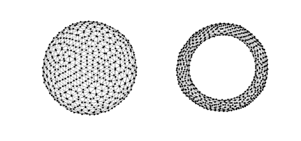
Figure 1: Two connected graphs on the surfaces of the unit sphere (left) and a torus (right). The left has 480 nodes and 1434 edges, and the right has 640 nodes and 1920 edges. The average vertex degree is 6.

For simplicity, we consider $m=1$ which means $A=\Delta_{G}$ is the Laplacian of the graph $G$. Performances of Jacobi, GS and SGS iterations for the original SPD system 82 and the augmented system 83 are reported in Tables 1 and 2. Also, results of PCG (i.e., Algorithm 4) with Jacobi and SGS preconditioners for the augmented system 83 are given. All the iterations are stopped either the maximal iteration number 1e5 is attained or the relative residual is smaller than 1e-6.

Table 1: Performances of iterative solvers for 82 and 83, related to the graph on the unit sphere in Fig. 1. Here, $\times$ means the maximal iteration number 1e5 is attained while the relative residual is larger than 1e-6.

		82							83
$\epsilon$		Jacobi		GS		SGS			Jacobi		GS		SGS		PCG-Jacobi		PCG-SGS
$1e$-1		746		375		212			232		113		66		30		16
$1e$-2		7439		3740		2104			427		214		117		39		19
$1e$-3		74358		37463		20968			461		237		134		41		19
$1e$-4		$\times$		$\times$		$\times$			479		241		131		41		19
$1e$-6		$\times$		$\times$		$\times$			468		236		131		41		19
$1e$-8		$\times$		$\times$		$\times$			468		233		131		41		19
0		473		235		134			-		-		-		-		-

It is observed that all the iterations for the augmented system 83 are robust with respect to $\epsilon$, and PCG with SGS preconditioner performances the best. However, we have to mention that, in the setting of decentralized distributed optimization, both GS and SGS iterations may not be preferable since all the nodes are updated sequentially. The Jacobi iteration 84 is parallel but another issue, which also exists in the GS iteration 85, is that there comes an additional variable $\widehat{v}_{1}\in\,{\mathbb{R}}$, which is updated via the average of $\widehat{\bm{v}}_{2}$. Moreover, to recover ${\bm{v}}_{k+1}=\widehat{v}_{1}{\bf 1}_{q}+\widehat{\bm{v}}_{2}$, all nodes need it. This can be done by introducing a master node that connects all other nodes and is responsible for updating $\widehat{v}_{1}$ and then sending it back to local nodes. Note again that both $\widehat{v}_{1}$ and $\widehat{\bm{v}}_{2}$ can be obtained simultaneously for Jacobi iteration. Therefore, the master and other nodes are allowed to be asynchronized. This maintains the decentralized nature of distributed optimization.

Table 2: Performances of iterative solvers for 82 and 83, related to the graph on the torus in Fig. 1. Here, $\times$ means the maximal iteration number 1e5 is attained while the relative residual is larger than 1e-6.

		82							83
$\epsilon$		Jacobi		GS		SGS			Jacobi		GS		SGS		PCG-Jacobi		PCG-SGS
$1e$-1		751		378		216			319		167		92		35		17
$1e$-2		7463		3759		2147			1031		526		294		57		22
$1e$-3		74825		37673		21408			1356		684		384		59		27
$1e$-5		$\times$		$\times$		$\times$			1396		708		399		60		27
$1e$-7		$\times$		$\times$		$\times$			1397		707		396		59		27
$1e$-9		$\times$		$\times$		$\times$			1396		701		400		60		27
0		1156		634		318			-		-		-		-		-

We have not presented convergence analysis in inexact setting but for all the forthcoming numerical tests in Sections 7.2 and 7.3, we adopt Algorithm 4 with Jacobi preconditioner and the tolerance $\varepsilon=\|A{\bm{x}}_{k}\|/10$ to solve the augmented system 83; see step 6 in Algorithm 7.

7.2 Decentralized least squares

Let us now consider the decentralized least squares

$$\min_{x\in\,{\mathbb{R}}^{m}}\frac{1}{n}\sum_{i=1}^{n}f_{i}(x)=\frac{1}{n}\sum_{i=1}^{n}\frac{1}{2}\left\lVert{B_{i}x-b_{i}}\right\rVert^{2},$$ (86)

where $B_{i}\in\,{\mathbb{R}}^{p\times m}$ and $b_{i}\in\,{\mathbb{R}}^{p}$ are randomly generated at each node $i$. Here we set $m=200$ and the sample number $p=5$. Note that each $f_{i}$ in 86 is smooth convex with $\mu_{i}=0$ and $L_{i}=\left\lVert{B_{i}}\right\rVert^{2}$, and for $f(\bm{x})=\frac{1}{n}\sum_{i=1}^{n}f_{i}(\bm{x}(i))$, we have $f\in\mathcal{S}_{0,L}^{1,1}$ with $L=\max\{L_{i}\}/n$.

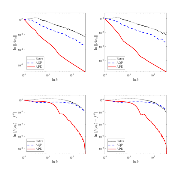
Figure 2: Convergence behaviors of Algorithm 7, Extra and AQP for problem 86 on the sphere graph (left) and the torus graph (right). Here $f^{\#}$ is the approximated optimal objective value.

We compare Algorithm 7 with Extra [59] and the accelerated quadratic penalty (AQP) method [35] for solving 86 with respect to the previous two connected graphs (plotted in Fig. 1). Starting from the problem 79, Extra requires the so-called mixing matrix $W$, which is related to the underlying graph $G$ and satisfies [59, Assumption 1], and it repeats the iteration procedure below

$$\left\{\begin{aligned} {}&{\bm{e}}_{k}=\bm{x}_{k}-\left(\widehat{W}\otimes I_{m}\right)\bm{x}_{k-1}+\alpha\nabla f(\bm{x}_{k-1}),\\ {}&\bm{x}_{k+1}=\left(W\otimes I_{m}\right)\bm{x}_{k}-\alpha\nabla f(\bm{x}_{k})+{\bm{e}}_{k},\end{aligned}\right.$$ (87)

for $k\geqslant 1$, where $\widehat{W}=(I+W)/2$ and the initial step is $\bm{x}_{1}={}\left(W\otimes I_{m}\right)\bm{x}_{0}-\alpha\nabla f(\bm{x}_{0})$. Assuming the spectrum of $W$ lies in $(-1,1]$ and that $\alpha=\lambda_{\min}(\widehat{W})/L$, [59, Theorem 3.5] gave the ergodic sublinear rate $O(1/k)$ for 87. The AQP method [35, Eq.(9)] rewrites 86 as the form 81 with $A=(I-U)/2\otimes I_{m}$ and performs the following iteration

$$\left\{\begin{aligned} {}&{\bm{y}}_{k}={\bm{x}}_{k}+\frac{k-1}{k+1}(\bm{x}_{k}-\bm{x}_{k-1}),\\ {}&\bm{x}_{k+1}={\bm{y}}_{k}-\frac{\nabla f({\bm{y}}_{k})+(k+1)A{\bm{y}}_{k}}{L+k+1},\end{aligned}\right.$$ (88)

for all $k\geqslant 1$, where $U$ is some symmetric doubly stochastic matrix such that $U_{ij}>0$ if and only of $(i,j)\in E$. The nonergodic convergence rate $O(1/k)$ for 88 has been established in [35, Theorem 6].

In this example and the next one, we choose $W=U=I-\Delta_{G}/\tau$ with $\tau=\lambda_{\max}(\Delta_{G})$. Then $W$ fulfills [59, Assumption 1] and by [4, Theorem 4.12], such $U$ also meets the requirement in 88. In Fig. 2, we plot the convergence behaviors of Extra, AQP and APD (Algorithm 7). By Theorem 5.1, APD converges with a faster sublinear rate $O(1/k^{2})$ and numerical results illustrate that our method outperforms the others indeed.

7.3 Decentralized logistic regression

We then look at the regularized decentralized logistic regression

$$\min_{x\in\,{\mathbb{R}}^{m}}\frac{1}{n}\sum_{i=1}^{n}f_{i}(x)=\frac{1}{n}\sum_{i=1}^{n}\left(\ln\left(1+\exp\left(-b_{i}\theta_{i}^{\top}x\right)\right)+\frac{\delta}{2}\left\lVert{x}\right\rVert^{2}\right),$$ (89)

where $\delta>0$ stands for the regularize parameter, $\theta_{i}\in\,{\mathbb{R}}^{m}$ is the data variable and $b_{i}\in\{-1,1\}$ denotes the binary class. Here we take $\delta=0.5$ and $m=300$. Note that each $f_{i}$ is smooth strongly convex and an elementary computation gives $\mu_{i}=\delta$ and $L_{i}=\delta+|b_{i}|^{2}\left\lVert{\theta_{i}}\right\rVert^{2}/4$. Hence $f(\bm{x})=\frac{1}{n}\sum_{i=1}^{n}f_{i}(\bm{x}(i))$ is also smooth strongly convex with $\mu=\delta/n$ and $L=\max\{L_{i}\}/n$.

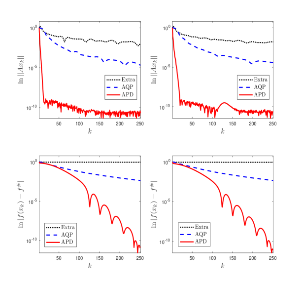
Figure 3: Convergence behaviors of Algorithm 7, Extra and AQP for problem 89 on the sphere graph (left) and the torus graph (right). Here $f^{\#}$ is the approximated optimal objective value.

In this case, the corresponding variant of AQP 88 has the theoretical sublinear rate $O(1/k^{2})$ and reads as follows

$$\left\{\begin{aligned} {}&{\bm{y}}_{k}={\bm{x}}_{k}+\frac{(\eta_{k}\theta_{k}-\mu\theta^{2}_{k})(1-\theta_{k-1})}{(\eta_{k}-\mu\theta^{2}_{k})\theta_{k-1}}(\bm{x}_{k}-\bm{x}_{k-1}),\\ {}&\bm{x}_{k+1}={\bm{y}}_{k}-\eta_{k}^{-1}\left(\theta^{2}_{k}\nabla f({\bm{y}}_{k})+\mu A{\bm{y}}_{k}\right),\end{aligned}\right.$$ (90)

where $\eta_{k}=L\theta_{k}^{2}+\mu$ and $\theta_{k}^{2}+\theta_{k-1}^{2}\theta_{k}=\theta_{k-1}^{2}$ with $\theta_{0}=1$. By [59, Theorem 3.7], Extra 87 has linear convergence with the step size $\alpha=\mu\lambda_{\min}(\widehat{W})/L^{2}$. However, numerical outputs in Fig. 3 show it performances even worse than AQP 90. This may be due to that the mixing matrix $W$ in 87 is not chosen properly and not much efficient for information diffusion in the graph. There are some alternative choices summarized in [59, Section 2.4] and we tried the Metropolis constant edge weight matrix, which performs not much better either and is not displayed here. We would not look at more mixing matrices beyond. To conclude, we observe fast linear convergence of APD (Algorithm 7) from Fig. 3, for both the objective gap and the feasibility.

8 Concluding Remarks

In this work, for minimizing a convex objective with linear equality constraint, we introduced a novel second-order dynamical system, called accelerated primal-dual flow, and proved its exponential decay property in terms of a suitable Lyapunov function. It was then discretized via different type of numerical schemes, which give a class of accelerated primal-dual algorithms for the affine constrained convex optimization problem 1.

The explicit scheme 70d corresponds to fully linearized proximal ALM and semi-implicit discretizations (cf. 39c and 53d) are close to partially linearized ALM. The subproblem of 53d has special structure and can be used to develop efficient inner solvers. Also, nonergodic convergence rates have been established via a unified discrete Lyapunov function. Moreover, the semi-implicit method 53d has been applied to decentralized distributed optimization and performances better than the methods in [35, 59].

Our differential equation solver approach provides a systematically way to design new primal-dual methods for problem 1, and the tool of Lyapunov function renders an effective way for convergence analysis. For future works, we will pay attention to the solution existence and the exponential decay for our APD flow system 10c in general nonsmooth setting. Besides, convergence analysis under inexact computation shall be considered as well.

At last, it is worth extending the current continuous model together its numerical discretizations to two block case 2. As discussed in Remark 4.3, both the semi-implicit discretization 39c and the explicit one 70d can be applied to the two block case 2 and lead to parallel ADMM-type methods. However, to get the rate $O(1/k^{2})$, they require strong convexity of $f$. Hence, it would also be our ongoing work for developing new accelerated primal-dual splitting methods that can handle partially strongly convex objectives.

References

[1]
H. Attouch, G. Buttazzo, and G. Michaille.
Variational Analysis in Sobolev and BV Spaces, 2nd.
MOS-SIAM Series on Optimization. Society for Industrial and Applied
Mathematics, 2014.
[2]
H. Attouch, Z. Chbani, J. Fadili, and H. Riahi.
Fast convergence of dynamical ADMM via time scaling of damped
inertial dynamics.
J. Optim. Theory Appl.,
https://doi.org/10.1007/s10957-021-01859-2, 2021.
[3]
H. Attouch, Z. Chbani, and H. Riahi.
Fast proximal methods via time scaling of damped inertial dynamics.
SIAM J. Optim., 29(3):2227–2256, 2019.
[4]
R. Bapat.
Graphs and Matrices, 2nd.
Universitext. Springer, London, 2014.
[5]
H. Bauschke and P. Combettes.
Convex Analysis and Monotone Operator Theory in Hilbert
Spaces.
CMS Books in Mathematics. Springer Science+Business Media, New York,
2011.
[6]
A. Beck.
First-Order Methods in Optimization, volume 1 of MOS–SIAM Series on Optimization.
Society for Industrial and Applied Mathematics and the Mathematical
Optimization Society, 2017.
[7]
R. I. Boţ and D.-K. Nguyen.
Improved convergence rates and trajectory convergence for primal-dual
dynamical systems with vanishing damping.
arXiv:2106.12294, 2021.
[8]
S. Boyd, N. Parikh, E. Chu, B. Peleato, and J. Eckstein.
Distributed optimization and statistical learning via the alternating
direction method of multipliers.
Foundations and Trends® in Machine Learning, 3(1):1–122,
2010.
[9]
A. Chambolle and T. Pock.
A first-order primal-dual algorithm for convex problems with
applications to imaging.
J.Math. Imaging Vis., 40(1):120–145, 2011.
[10]
A. Chambolle and T. Pock.
On the ergodic convergence rates of a first-order primal–dual
algorithm.
Math. Program., 159(1-2):253–287, 2016.
[11]
C. Chen, B. He, Y. Ye, and X. Yuan.
The direct extension of ADMM for multi-block convex minimization
problems is not necessarily convergent.
Math. Program., 155:57–79, 2016.
[12]
G. Chen and M. Teboulle.
A proximal-based decomposition method for convex minimization
problems.
Math. Program., 64(1), 1994.
[13]
L. Chen and H. Luo.
First order optimization methods based on Hessian-driven Nesterov
accelerated gradient flow.
arXiv:1912.09276, 2019.
[14]
F. Clarke.
Optimization and Nonsmooth Analysis.
Number 5 in Classics in Applied Mathematics. Society for
Industrial and Applied Mathematics, 1987.
[15]
J. E. Dennis and R. B. Schnabel.
Numerical Methods for Unconstrained Optimization and
Nonlinear Equations.
Number 16 in Classics in applied mathematics. Society for Industrial
and Applied Mathematics, Philadelphia, 1996.
[16]
F. Facchinei and J. Pang.
Finite-Dimensional Variational Inequalities and Complementarity
Problems, vol 2.
Springer, New York, 2003.
[17]
G. França, D. P. Robinson, and R. Vidal.
ADMM and accelerated ADMM as continuous dynamical systems.
arXiv:1805.06579, 2018.
[18]
G. França, D. P. Robinson, and R. Vidal.
A nonsmooth dynamical systems perspective on accelerated extensions
of ADMM.
arXiv:1808.04048, 2021.
[19]
T. Goldstein, B. O’Donoghue, S. Setzer, and R. Baraniuk.
Fast alternating direction optimization methods.
SIAM J. Imaging Sci., 7(3):1588–1623, 2014.
[20]
D. Han, D. Sun, and L. Zhang.
Linear rate convergence of the alternating direction method of
multipliers for convex composite quadratic and semi-definite programming.
arXiv:1508.02134, 2015.
[21]
B. He and X. Yuan.
On the acceleration of augmented Lagrangian method for linearly
constrained optimization.
2010.
[22]
B. He and X. Yuan.
On the convergence rate of the Douglas–Rachford
alternating direction method.
SIAM J. Numer. Anal., 50(2):700–709, 2012.
[23]
B. He and X. Yuan.
On non-ergodic convergence rate of Douglas–Rachford alternating
direction method of multipliers.
Numer. Math., 130(3):567–577, 2015.
[24]
X. He, R. Hu, and Y.-P. Fang.
Convergence rates of inertial primal-dual dynamical methods for
separable convex optimization problems.
arXiv:2007.12428, 2020.
[25]
X. He, R. Hu, and Y.-P. Fang.
Convergence rate analysis of fast primal-dual methods with scalings
for linearly constrained convex optimization problems.
arXiv:2103.10118, 2021.
[26]
X. He, R. Hu, and Y.-P. Fang.
Fast convergence of primal-dual dynamics and algorithms with time
scaling for linear equality constrained convex optimization problems.
arXiv:2103.1293, 2021.
[27]
X. He, R. Hu, and Y.-P. Fang.
Inertial primal-dual methods for linear equality constrained convex
optimization problems.
arXiv:2103.12937, 2021.
[28]
X. He, R. Hu, and Y.-P. Fang.
Perturbed primal-dual dynamics with damping and time scaling
coefficients for affine constrained convex optimization problems.
arXiv:2106.13702, 2021.
[29]
M. R. Hestenes.
Multiplier and gradient methods.
J. Optim. Theory Appl., 4(5):303–320, 1969.
[30]
B. Huang, S. Ma, and D. Goldfarb.
Accelerated linearized Bregman method.
J. Sci. Comput., 54:428–453, 2013.
[31]
M. Kang, M. Kang, and M. Jung.
Inexact accelerated augmented Lagrangian methods.
Comput. Optim. Appl., 62(2):373–404, 2015.
[32]
M. Kang, S. Yun, H. Woo, and M. Kang.
Accelerated Bregman method for linearly constrained
- minimization.
J. Sci. Comput., 56(3):515–534, 2013.
[33]
G. Lan and R. Monteiro.
Iteration-complexity of first-order penalty methods for convex
programming.
Math. Program., 138(1-2):115–139, 2013.
[34]
Y. Lee, J. Wu, J. Xu, and L. Zikatanov.
Robust subspace correction methods for nearly singular systems.
Mathematical Models and Methods in Applied Sciences,
17(11):1937–1963, 2007.
[35]
H. Li, C. Fang, and Z. Lin.
Convergence rates analysis of the quadratic penalty method and its
applications to decentralized distributed optimization.
arXiv:1711.10802, 2017.
[36]
H. Li and Z. Lin.
Accelerated alternating direction method of multipliers: An optimal
nonergodic analysis.
J. Sci. Comput., 79(2):671–699, 2019.
[37]
X. Li, D. Sun, and K.-C. Toh.
A highly efficient semismooth Newton augmented Lagrangian method
for solving Lasso problems.
SIAM J. Optim., 28(1):433–458, 2018.
[38]
X. Li, D. Sun, and K.-C. Toh.
An asymptotically superlinearly convergent semismooth Newton
augmented Lagrangian method for Linear Programming.
arXiv:1903.09546, 2020.
[39]
T. Lin, S. Ma, and S. Zhang.
Iteration complexity analysis of multi-block ADMM for a family of
convex minimization without strong convexity.
arXiv:1504.03087, 2015.
[40]
Y. Liu, X. Yuan, S. Zeng, and J. Zhang.
Partial error bound conditions and the linear convergence rate of the
alternating direction method of multipliers.
SIAM J. Numer. Anal., 56(4):2095–2123, 2018.
[41]
H. Luo.
Accelerated differential inclusion for convex optimization.
arXiv:2103.06629, 2021.
[42]
H. Luo.
A primal-dual flow for affine constrained convex optimization.
arXiv:2103.06636, 2021.
[43]
H. Luo and L. Chen.
From differential equation solvers to accelerated first-order methods
for convex optimization.
Math. Program., https://doi.org/10.1007/s10107-021-01713-3, 2021.
[44]
Y. Nesterov.
A method of solving a convex programming problem with convergence
rate .
Soviet Mathematics Doklady, 27(2):372–376, 1983.
[45]
Y. Nesterov.
Excessive gap technique in nonsmooth convex minimization.
SIAM J. Optim., 16(1):235–249, 2005.
[46]
Y. Nesterov.
Smooth minimization of non-smooth functions.
Math. Program., 103(1):127–152, 2005.
[47]
Y. Nesterov.
Gradient methods for minimizing composite functions.
Math. Program. Series B, 140(1):125–161, 2013.
[48]
Y. Nesterov.
Lectures on Convex Optimization, volume 137 of Springer Optimization and Its Applications.
Springer International Publishing, Cham, 2018.
[49]
D. Niu, C. Wang, P. Tang, Q. Wang, and E. Song.
A sparse semismooth Newton based augmented Lagrangian method for
large-scale support vector machines.
arXiv:1910.01312, 2021.
[50]
A. Padiy, O. Axelsson, and B. Polman.
Generalized augmented matrix preconditioning approach and its
application to iterative solution of ill-conditioned algebraic systems.
SIAM J. Matrix Anal. & Appl., 22(3):793–818, 2001.
[51]
A. Patrascu, I. Necoara, and Q. Tran-Dinh.
Adaptive inexact fast augmented Lagrangian methods for constrained
convex optimization.
Optimization Letters, 11(3):609–626, 2017.
[52]
P. Persson and G. Strang.
A simple mesh generator in MATLAB.
SIAM Rev., 46(2):329–345, 2004.
[53]
L. Qi.
Convergence analysis of some algorithms for solving nonsmooth
equations.
Math. Oper. Res., 18(1):227–244, 1993.
[54]
L. Qi and J. Sun.
A nonsmooth version of Newton’s method.
Math. Program., 58(1-3):353–367, 1993.
[55]
R. T. Rockafellar.
Augmented Lagrangians and applications of the proximal point
algorithm in convex programming.
Mathematics of OR, 1(2):97–116, 1976.
[56]
S. Sabach and M. Teboulle.
Faster Lagrangian-based methods in convex optimization.
arXiv:2010.14314, 2020.
[57]
A. Salim, L. Condat, D. Kovalev, and P. Richtárik.
An optimal algorithm for strongly convex minimization under affine
constraints.
arXiv:2102.11079, 2021.
[58]
J. Shewchuk.
An introduction to the conjugate gradient method without the
agonizing, edition 5/4.
Technical report, Carnegie Mellon University, Pittsburgh, PA, USA,
1994.
[59]
W. Shi, Q. Ling, G. Wu, and W. Yin.
Extra: An exact first-order a lgorithm for decentralized consensus
optimization.
SIAM J. Optim., 25(2):944–966, 2015.
[60]
W. Su, S. Boyd, and E. Candès.
A differential equation for modeling Nesterov’s accelerated
gradient method: theory and insights.
J. Mach. Learn. Res., 17:1–43, 2016.
[61]
M. Tao and X. Yuan.
Accelerated Uzawa methods for convex optimization.
Math. Comp., 86(306):1821–1845, 2016.
[62]
Q. Tran-Dinh and V. Cevher.
Constrained convex minimization via model-based excessive gap.
In In Proc. the Neural Information Processing Systems
(NIPS), volume 27, pages 721–729, Montreal, Canada, 2014.
[63]
Q. Tran-Dinh and V. Cevher.
A primal-dual algorithmic framework for constrained convex
minimization.
arXiv:1406.5403, 2015.
[64]
Q. Tran-Dinh, O. Fercoq, and V. Cevher.
A smooth primal-dual optimization framework for nonsmooth composite
convex minimization.
SIAM J. Optim., 28(1):96–134, 2018.
[65]
P. Tseng.
On accelerated proximal gradient methods for convex-concave
optimization.
Technical report, University of Washington, Seattle, 2008.
[66]
J. Xu.
The method of subspace corrections.
J.Comput. Applied Math., 128:335–362, 2001.
[67]
Y. Xu.
Accelerated first-order primal-dual proximal methods for linearly
constrained composite convex programming.
SIAM J. Optim., 27(3):1459–1484, 2017.
[68]
W. Yin, S. Osher, D. Goldfarb, and J. Darbon.
Bregman iterative algorithms for -minimization with
applications to compressed sensing.
SIAM J. Imaging Sci., 1(1):143–168, 2008.
[69]
X. Yuan, S. Zeng, and J. Zhang.
Discerning the linear convergence of ADMM for structured convex
optimization through the lens of variational analysis.
J. Mach. Learn. Res., 21:1–74, 2020.
[70]
X. Zeng, J. Lei, and J. Chen.
Dynamical primal-dual accelerated method with applications to network
optimization.
arXiv:1912.03690, 2019.
[71]
X. Zeng, P. Yi, Y. Hong, and L. Xie.
Distributed continuous-time algorithms for nonsmooth extended
monotropic optimization problems.
SIAM J. Control Optim., 56(6):3973–3993, 2018.