Controlling reaction dynamics in chemical model systems through external driving

Abstract

The rate of a chemical reaction can often be determined by the properties of a rank-1 saddle and the associated transition state separating reactants and products. We have found evidence that such rates can be controlled and even enhanced by external driving in at least one such system. Specifically, we analyze a reactive model in two degrees of freedom that has been used earlier to describe driven chemical reactions. Therein, changes in the external driving can lead to a local maximum of the decay rate constant or even to bifurcations of periodic trajectories on the normally hyperbolic invariant manifold (NHIM) corresponding to the transition state. Inspired by these bifurcations, we show that in this case, the dynamics on the NHIM can be connected to the geometry of reactive trajectories and to reaction probabilities of Maxwell–Boltzmann distributed reactant ensembles.

1 Introduction

Reactant and product states in a chemical reaction are usually separated by a barrier that needs to be surmounted during the reaction. Dynamics near the barrier have been successfully described by the framework of transition state theory (TST) [1, 2, 3, 4, 5, 6, 7, 8]. Beyond the reactants and products, TST focuses on the determination of the transition state (TS), an unstable state confined indefinitely at the transition barrier that is neither reactant nor product. Alternatively, one could focus on the correlation between the respective fluxes through the dividing surfaces associated with the reactants and products as they enter the flux correlation formalism for the rate formula [9]. The determination of the transition paths between such surfaces has recently been used as the basis of accurate rate formulas in a non-driven system [10]. Here, instead, we focus on the use of the TS as the barrier separating reactants from products. In arbitrary dimensions, the TS is embedded in the normally hyperbolic invariant manifold (NHIM) of the associated barrier region separating reactants from products [11, 12]. As the name suggests, reactants need to pass close to this TS in order to react. Therefore, it should not be surprising that a dividing surface (DS) separating reactants from products can be attached to the NHIM [13, 14, 5, 6, 15].

Recent advances in the use of TSs to obtain chemical reaction rates include the resolution of classical model systems [5, 16, 17, 18, 19, 20, 21, 8, 22, 23, 24, 25, 26] of varying complexity as well as quantum mechanical problems [27]. Most of these problems feature transitions over a rank-1 saddle along a confined reaction pathway in a time-independent system invariably using perturbative expansions. As not all systems admit to such solutions, we have also pursued alternate approaches, including Lagrangian descriptors [28, 29, 30], binary contraction [31], and machine learning [32]. In this paper, we address the emergent dynamics of a time-dependent chemical model system under periodic external driving of the transition barrier. We find in Secs. 3.1 and 3.2 that our model admits to a decay rate that is highly sensitive to the strength and frequency of the driving, and hence the decay rate can be controlled. In the process, the structure of the NHIM changes qualitatively via bifurcations. Section 3.3 further analyzes one such bifurcation and how it influences reactive trajectories passing close to the NHIM. The results allow us to predict reaction probabilities in Sec. 3.4. These sections clarify how the dynamics on the NHIM translates to reactive properties of ensembles starting far from it.

2 Materials and methods

We represent driven chemical reactions using a model explored in previous work [30, 32, 31, 33, 34, 35]. As in typical chemical reactions, the barrier region is represented as a rank-1 saddle separating reaction and product basins such as shown in the contour plots of Fig. 1. The driving arises by way of coupling between a time-dependent external field and the dipole associated with the reaction coordinate [36, 37]. Besides being physically relevant to chemical reactions, the restriction to unbounded reactant and product basins is a simplification that avoids the global recrossings that would arise if one or both basins were closed. Nevertheless, we emphasize that the presence of closed reactant and product basins would not challenge the methods presented here because the important dynamics is happening in the saddle region. For more information on how to deal with global recrossings see Ref. [38].

2.1 Model potential

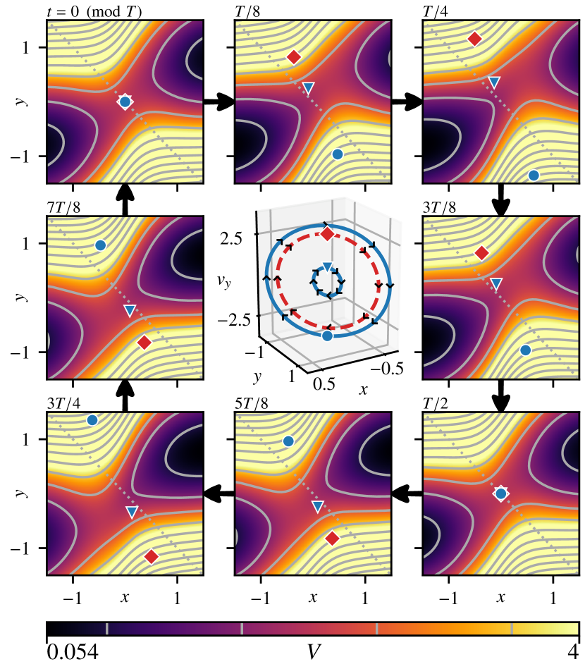
Figure 1: Outer ring: Snapshots of the time-dependent potential $V(x,y,t)$ following Eq. (1) with $\omega_{x}=$0.77$\,\pi$ and $\hat{x}=$0.4$$ over the oscillation period $T=2\pi/\omega_{x}$. Diamond, triangle, and circle markers symbolize the position of three particles with trajectories of period $T$. Equidistant contour lines with $\Delta V=1$ are shown in solid gray. A diagonal dotted line per panel serves as a guide to the eye, elucidating the saddle movement. The color scale is capped at $V=4$. Center: Aforementioned periodic trajectories in phase space. Filled markers symbolize positions at $t=0$ while positions of the particles at the potential snapshots are indicated by black arrow heads pointing in the direction of motion.

In more detail, we use a two-dimensional potential

$$\begin{split}V(x,y,t)&=E_{\mathrm{b}}\exp(-\quantity[x-\hat{x}\sin(\omega_{x}t)]^{2})\\ &\quad+\frac{\omega_{y}^{2}}{2}\quantity[y-\frac{2}{\pi}\arctan(2x)]^{2}\,\text{,}\end{split}$$ (1)

where a time-periodically oscillating Gaussian barrier with height $E_{\mathrm{b}}$ separates an unbounded reactant from an unbounded product basin, as shown in Fig. 1. The barrier moves along the $x$-coordinate with frequency $\omega_{x}$ and amplitude $\hat{x}$. In the $y$-direction, the particles are bound by a harmonic potential with frequency $\omega_{y}$. To make the system nonlinear, the $x$ and $y$ coordinates are coupled so that the minimum energy path for a reaction over the saddle is given by $y=(2/\pi)\arctan(2x)$. For simplicity, we use dimensionless units with parameters $E_{\mathrm{b}}=$2$$ and $\omega_{y}=$2$$. The aim of this work is to demonstrate how chemical reactions can be controlled by external driving. We focus on the dependence of the system on the parameters $\omega_{x}$ and $\hat{x}$ since they describe the saddle movement caused by the external driving.

2.2 Decay rates

To calculate the decay rate associated with trajectories on the NHIM, we use the Floquet method first introduced in Ref. [39] and later extended in Refs. [40, 11, 34]. The method relies on the conjecture—verified under certain assumptions such as those shown here—that the decay rate of reactants into products near a TS is related to the Floquet coefficients of the TS. It exploits the fact that trajectories near a periodic orbit on the NHIM can be described using a linearization of the equations of motion. Let $\Delta\bm{\gamma}(t)$ represent the deviation of a trajectory from the orbit with period $T_{\mathrm{po}}$. Its time evolution can then be described by

$$\Delta\dot{\bm{\gamma}}(t)=\bm{J}(t)\Delta\bm{\gamma}(t)$$ (2)

where $\bm{J}(t)$ is the system’s Jacobian evaluated on the periodic orbit. By leveraging its linearity, Eq. (2) can also be expressed as

$$\Delta\bm{\gamma}(t)=\bm{\sigma}(t)\Delta\bm{\gamma}(0)$$ (3)

where the fundamental matrix $\bm{\sigma}(t)$ is defined by

$$\dot{\bm{\sigma}}(t)=\bm{J}(t)\bm{\sigma}(t)\mbox{\quad with\quad}\bm{\sigma}(0)=\bm{1}$$ (4)

and $\bm{1}$ being the identity matrix. The rate constant $\bar{k}_{\mathrm{F}}$ then follows from the largest and smallest eigenvalue $m_{\mathrm{u,s}}(t)$ of $\bm{\sigma}(t)$ as

$$\bar{k}_{\mathrm{F}}T_{\mathrm{po}}=\ln|m_{\mathrm{u}}(T_{\mathrm{po}})|-\ln|m_{\mathrm{s}}(T_{\mathrm{po}})|\,\text{.}$$ (5)

This method can be generalized to non-periodic trajectories by evaluating the right-hand side of Eq. (5) for sufficiently long times and then applying a linear regression [11].

3 Results and discussion

We start by investigating two examples in which the external driving can be seen to affect the dynamics of the activated complex. In the following, we use $\expectationvalue{X}_{Y}$ to denote the average of quantity $X(Y)$ over $Y$.

3.1 Dynamics on the NHIM

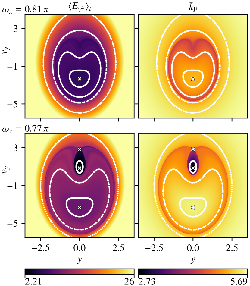
Figure 2: Average total energy $\expectationvalue*{E_{\gamma^{\ddagger}}}_{t}$ (left column, capped at $\expectationvalue*{E_{\gamma^{\ddagger}}}_{t}=$26$$) and rate constant $\bar{k}_{\mathrm{F}}$ (right column) of trajectories $\gamma^{\ddagger}$ started at position $(y,v_{y})$ and time $t_{0}=0$ on the NHIM. Shown are typical plots at $\hat{x}=$0.4$$ before (top row, $\omega_{x}=$0.81$\,\pi$) and after (bottom row, $\omega_{x}=$0.77$\,\pi$) the bifurcation. To elucidate the structure, a stroboscopic map of selected trajectories (PSOS, white dots) has been overlaid highlighting the existence of one elliptic fixed point before and two elliptic as well as one hyperbolic fixed point after the bifurcation (small white crosses). While the elliptic fixed points are always characterized by local minima in $\expectationvalue*{E_{\gamma^{\ddagger}}}_{t}$, they feature either a local minimum or maximum in $\bar{k}_{\mathrm{F}}$.

The left column of Fig. 2 shows the time-averaged total energy $\expectationvalue*{E_{\gamma^{\ddagger}}}_{t}$ of trajectories $\gamma^{\ddagger}$ on the NHIM for two values of $\omega_{x}$. At $\omega_{x}=$0.81$\,\pi$, $\expectationvalue*{E_{\gamma^{\ddagger}}}_{t}$ reveals a region in phase space with low-energy trajectories. This region is accompanied by a local maximum in the decay rate $\bar{k}_{\mathrm{F}}$, as can be seen in the right column of Fig. 2. The overlaid Poincaré surface of section (PSOS) highlights an elliptic fixed point belonging to the associated periodic orbit. This orbit fulfills all requirements for a TS trajectory as defined in Refs. [33, 11, 34]. It can be seen as the dominant trajectory in the sense that decay rates from this trajectory are also characteristic of neighboring trajectories.

For decreasing $\omega_{x}$, two new fixed points and, hence, periodic trajectories emerge, as can be seen in Fig. 2 at $\omega_{x}=$0.77$\,\pi$. These trajectories are shown in Fig. 1 for the elliptic (solid blue lines) and hyperbolic (dashed red line) fixed points. This so-called saddle-node bifurcation [41, 42, 43, 44, 35] qualitatively changes the dynamics on the NHIM. While the new elliptic fixed point is still characterized by a local minimum in $\expectationvalue*{E_{\gamma^{\ddagger}}}_{t}$, it now also features a local minimum in $\bar{k}_{\mathrm{F}}$ instead of a maximum. In addition, its energy $\expectationvalue*{E_{\gamma^{\ddagger}}}_{t}$ is much lower compared to the original elliptic fixed point at velocity $v_{y}=\dot{y}\approx$-3$$.

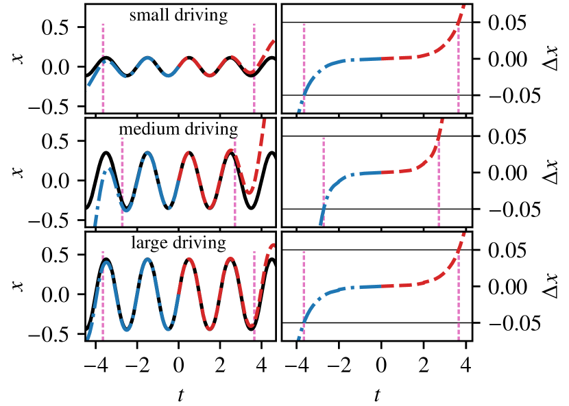
Figure 3: Position $x$ over time $t$ for three systems with small ($\hat{x}=$0.1$$), medium ($\hat{x}=$0.6$$), and large ($\hat{x}=$1.6$$) driving. Driving frequency in all cases is $\omega_{x}=\pi$. For each parameter set, the periodic trajectory (black solid) as well as a trajectory offset by $\Delta v_{x}=${10}^{-3}$$ at $t_{0}=0$ (blue dash dotted/red dashed) are shown. The stability of the trajectories is indicated in the right column by the time interval (vertical lines) where the deviation $\Delta x$ from the TS is less than $0.05$ (horizontal lines). Stability is minimal for medium driving.

The second example for the influence of external driving on the dynamics on the NHIM is illustrated in Fig. 3. At a fixed $\omega_{x}=\pi$, only a single periodic trajectory was found in the examined parameter regime. Particles near this periodic trajectory exhibit a change in their stability that depends on the system’s driving amplitude $\hat{x}$. We illustrate the change in the stability using the time it takes the particle to reach a distance of $\absolutevalue{\Delta x}=$0.05$$ from the periodic trajectory. When only a small driving is applied, the particle stays in the saddle region for a relatively long time. This in turn indicates a low decay rate $\bar{k}_{\mathrm{F}}$. When increasing the amplitude, stability initially decreases for medium driving only to increase again for large driving. As a result, there must be a local maximum in the systems decay rate $\bar{k}_{\mathrm{F}}$ allowing for rate enhancement through optimization of $\hat{x}$.

3.2 Decay rate enhancement

These two examples demonstrate that the dynamics of trajectories on or near the NHIM can be drastically altered through modification of the driving parameters. This is summarized in Fig. 4 through the calculation of the decay rates $\bar{k}_{\mathrm{F}}$ as a function of the driving frequency and amplitude. As these are only one-dimensional sections through the two-dimensional space of possible driving parameters, they serve here as examples only. Specifically, they are not meant to represent an exhaustive or exclusive set. As such, any extremal values in one of these sections may not necessarily be extremal in the full parameter space. Nevertheless, the existence of such extrema in sections of parameter space is enough to demonstrate that these systems are sensitive to the driving.

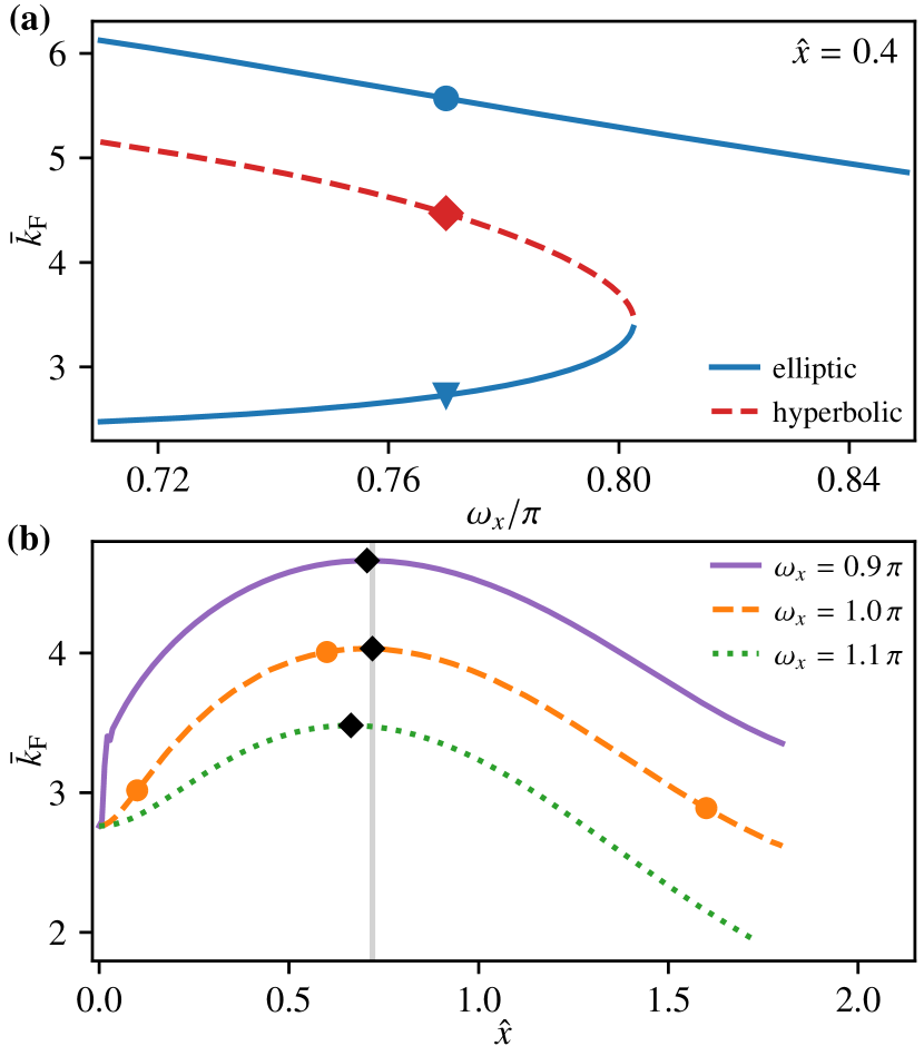
Figure 4: (a) Rate constant $\bar{k}_{\mathrm{F}}$ as a function of driving frequency $\omega_{x}$ for two elliptic and one hyperbolic fixed point, each corresponding to a periodic trajectory. At $\omega_{x}\approx$0.80$\,\pi$, two fixed points vanish in a saddle-node bifurcation. The three markers correspond to the trajectories shown in Fig. 1. (b) Rate constant $\bar{k}_{\mathrm{F}}$ as a function of driving amplitude $\hat{x}$ for three different driving frequencies $\omega_{x}$. Only a single fixed point (i. e., periodic trajectory) was found per set of parameters considered here. Orange circles indicate the parameter sets used in Fig. 3 while black diamonds mark each curve’s maximum. The vertical gray line acts as a guide to the eye.

The bifurcation observed in Fig. 2 is visible in Fig. 4(a). At larger driving frequencies, there exists a single elliptic fixed point. When lowering $\omega_{x}$, its rate constant $\bar{k}_{\mathrm{F}}$ steadily increases. Around $\omega_{x}=$0.80$\,\pi$, two new fixed points with lower values of $\bar{k}_{\mathrm{F}}$ emerge in a saddle-node bifurcation. Furthermore, a comparison with the trajectories from Fig. 1 suggests that high rates are accompanied by large motion in the orthogonal mode $(y,v_{y})$.

We demonstrated through Fig. 3 that there exists a minimum in stability for medium driving. This manifests itself in Fig. 4(b) by means of a maximum in $\bar{k}_{\mathrm{F}}$. When varying $\omega_{x}$, this extremum persists qualitatively the same, differing mainly in position and height. The latter can be connected to the slope in Fig. 4(a). Note that all curves, independent of $\omega_{x}$, must meet at $\bar{k}_{\mathrm{F}}(\hat{x}=0)\approx$2.762$$ since a vanishing amplitude is equivalent to the static case.

3.3 Reaction geometry

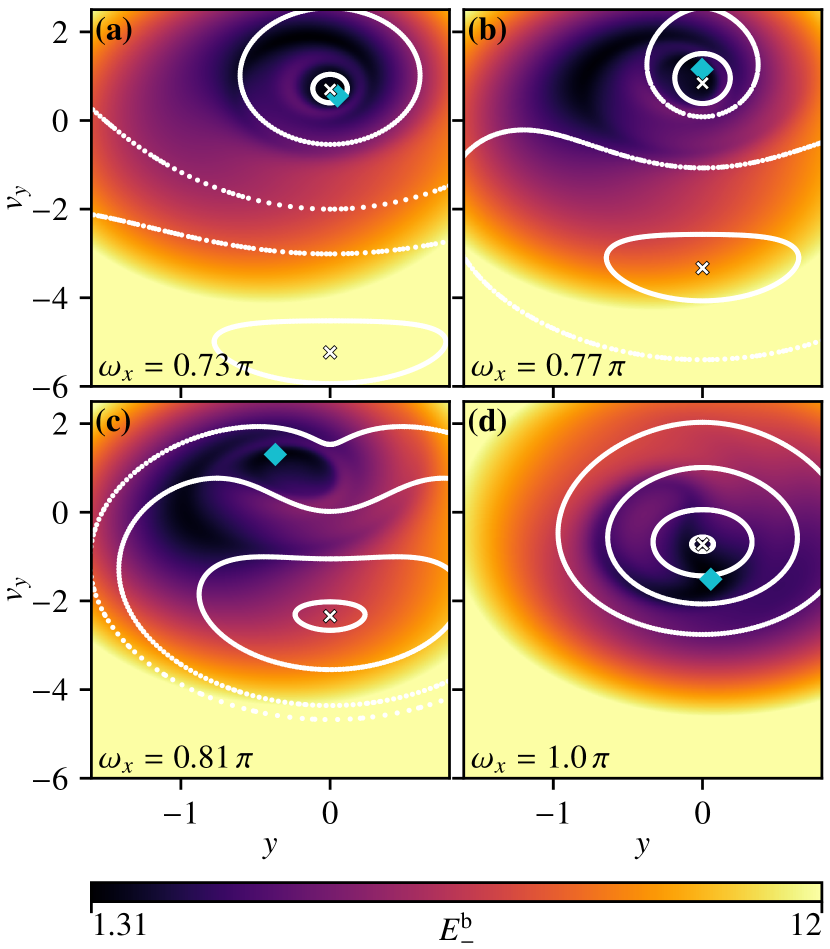
Figure 5: Local threshold energy $E_{-}^{\mathrm{b}}=\lim_{t\to-\infty}E_{\gamma}$ of trajectories $\gamma$ started from position $(y,v_{y})$ close to the NHIM at crossing time $t_{0}=0$ and propagated back to the initial time $t\to-\infty$. A PSOS showing the structure of the NHIM is overlaid for comparison. Small white crosses mark the positions of elliptic fixed points. The diamond marker in each panel is placed at the global spacial minimum $E_{\mathrm{th}}^{\mathrm{b}}(t_{0})=\min_{y,v_{y}}E_{-}^{\mathrm{b}}(y,v_{y},t_{0})$. The panels (a) through (d) were calculated for different driving frequencies $\omega_{x}$ as indicated in the bottom left of each panel. The driving amplitude is $\hat{x}=$0.4$$ for all panels. The color scale is capped at $E_{-}^{\mathrm{b}}=$12$$.

The results reported in the previous sections relate only to the dynamics on the NHIM. Making predictions about real chemical reactions, however, requires us to connect to the dynamics off the NHIM. More specifically, we need to address when and how the NHIM can influence reactive trajectories, i. e., those connecting the reactant to the product basins.

The NHIM represents—by construction—the minimum energy a trajectory needs for any given set of orthogonal modes $(y,v_{y})$ to cross the DS. It is therefore natural to assume that a significant portion of reactants in a thermally distributed ensemble would pass close to the NHIM while reacting. Additionally, for reasons of continuity, we can expect these trajectories to behave similarly to those on the NHIM for some finite time. This provides a possible connection between the dynamics on and off the NHIM.

In a driven system, reactants may gain or lose energy while climbing the potential barrier. A trajectory’s energy $E_{\gamma}$ very close to the NHIM can thus differ from its initial energy $E_{-}^{\mathrm{b}}=\lim_{t\to-\infty}E_{\gamma}$ in the reactant basin. The structure of the NHIM can be connected to the reactant basins through propagation back in time. For each fixed orthogonal mode $(y,v_{y})$ and time $t_{0}$, we first obtain the position $(x,v_{x})$ of the NHIM. A shift of this point by $\Delta v_{x}=+${10}^{-5}$$ yields a point on a reactive trajectory which closely passes the NHIM. We then propagate the trajectory backward in time until we are sufficiently far away from the moving barrier. The trajectory’s energy $E_{-}^{\mathrm{b}}$ at this early time—which we refer to as the local threshold energy—will then be approximately conserved. Through sampling $(y,v_{y})$, we then obtain the distribution of local threshold energies and the corresponding initial points in phase space of the reactive trajectories. Figure 5 reports the results of this calculation for crossing time $t_{0}=0$ at four driving frequencies $\omega_{x}$ around the bifurcation shown in Fig. 4. For comparison, the structure of the NHIM as revealed by a PSOS has been overlaid in each case.

The PSOS reveals two elliptic fixed points on the NHIM at the driving frequencies below the bifurcation [cf. Figs. 5(a) and 5(b)]. Although the lower one cannot be seen in the structure of the local threshold energy, there is a correlation between $E_{-}^{\mathrm{b}}$ and the upper fixed point. This is consistent with the fact that the lower fixed point is associated with higher decay rates as shown in Fig. 4. Trajectories consequently spend less time near the NHIM, and we expect less correlation with the dynamics on the NHIM. Conversely, there is a very good match between the global threshold energy

$$E_{\mathrm{th}}^{\mathrm{b}}(t_{0})=\min_{y,v_{y}}E_{-}^{\mathrm{b}}(y,v_{y},t_{0})$$ (6)

and the position of the upper fixed point, i. e., the trajectory on the NHIM with the least average energy (cf. Fig. 2).

Closer to the bifurcation, we find the structure of $E_{-}^{\mathrm{b}}$ starting to change [cf. Figs. 5(b) and 5(c)]. Low-energy regions seem to flow out in a counter-clockwise spiral-like structure. The minimum $E_{\mathrm{th}}^{\mathrm{b}}$, however, stays near the upper fixed point. It only starts to move once this fixed point disappears in the bifurcation. Following a counter-clockwise trajectory itself, it moves down towards the remaining fixed point, slowly converging for increasing driving frequency $\omega_{x}$ [cf. Fig. 5(d)].

If we assume initial energies of a reactant ensemble to be thermally distributed, then we can expect most of these reactants to react via paths related to low-$E_{-}^{\mathrm{b}}$ regions at the crossing time $t_{0}$. The bifurcation, therefore, should change the geometry of the reaction dynamics at least qualitatively. This change, as indicated by the movement of the global spacial minimum of the threshold energy $E_{\rm th}^{\rm b}(t_{0})$, appears to be smooth across the bifurcation. As a consequence, we can anticipate that the reaction rates to be presented in the next section will not exhibit a discontinuity around the bifurcation.

3.4 Reaction probability

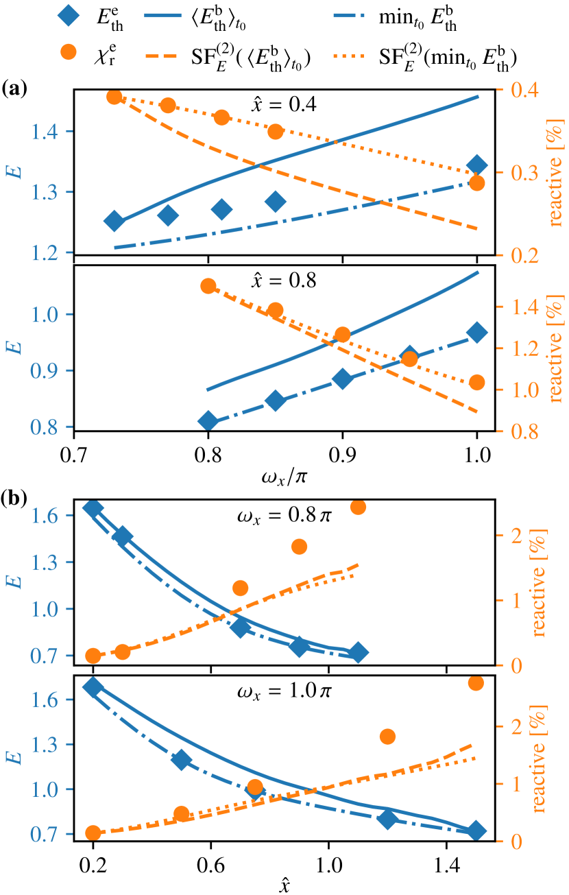
Figure 6: Ensemble threshold energy $E_{\mathrm{th}}^{\mathrm{e}}$ (diamond markers) and fraction of reactive trajectories $\chi_{\mathrm{r}}^{\mathrm{e}}$ (circle markers) for the ensemble calculation described in Sec. 3.4. Each of the four panels varies either (a) driving frequency $\omega_{x}$ or (b) driving amplitude $\hat{x}$ while the other parameter is kept fixed. For comparison, calculations based on the global minimum $E_{\mathrm{th}}^{\mathrm{b}}(t_{0})=\min_{y,v_{y}}E_{-}^{\mathrm{b}}(y,v_{y},t_{0})$ of the local threshold energy $E_{-}^{\mathrm{b}}$ akin to Fig. 5 are shown. Specifically, the average $\expectationvalue{E_{\mathrm{th}}^{\mathrm{b}}}_{t_{0}}$ and minimum $\min_{t_{0}}E_{\mathrm{th}}^{\mathrm{b}}$ in crossing time $t_{0}$ are shown with solid and dash-dotted lines, respectively. Evaluating the survival function $\mathrm{SF}_{E}^{(1)}$ of a one-dimensional Maxwell–Boltzmann distribution in energy space and scaling the results to fit the first ensemble data point yields the dashed and dotted lines, respectively. Parameter ranges differ because of numerical stability.

We now address the degree to which reaction rates—not just decay rates—can be obtained from the structure of the NHIM. Following Farkas and Kramers [45, 46, 47, 48], the reaction rate is determined by the ratio of the reactive flux across a DS divided by the reactant population at steady-state conditions. This presumes a boundary condition in which the reactants are continuously populated at the well according to an equilibrium condition. Here we assume that the reactants are initially thermally distributed, and set the initial distribution in velocities to be that of Boltzmann at temperature, $T$, and located in the reactant basin far from the NHIM. The system is then propagated semi-microcanonically—viz., including external driving but neglecting friction and noise. This corresponds to a system which is very weakly coupled to an external bath. The rates that one would obtain in this way are therefore good approximations in cases in which the rate is fast compared to the dissipation.

For numerical expedience, here we obtain the reaction fraction rather than the rates using the flux over population approach. The reactant fraction is the fraction of particles that react—before their first return to the reactant basin—to products given the initial distribution. The reference ensemble simulation is constructed as follows. For every set of parameters, we initialize an ensemble of ${10}^{7}$ reactants at position $(x,y)=(-8,-1)$, that is, far from the saddle on the minimum energy path. Velocities $v_{x}$ and $v_{y}$ are chosen according to a Maxwell–Boltzmann distribution of temperature $k_{\mathrm{B}}T=$0.4$\ll E_{\mathrm{b}}$. Negative velocities result in trajectories that cannot react because the reactant basin is unbounded. We thus include only positive velocities $v_{x}\geq 0$ by taking the absolute value. The initial time is chosen based on a uniform random distribution. Each reactant is then propagated forward in time until it leaves the reaction region. Trajectories passing $x<-8$ are classified as nonreactive and those passing $x>+4$ as reactive. Besides the fraction of reactive trajectories $\chi_{\mathrm{r}}^{\mathrm{e}}$, we additionally record the minimal initial energy $E_{\mathrm{th}}^{\mathrm{e}}$ of the reactive subensemble, referred to as the ensemble threshold energy. The results for various values of the driving parameters $\omega_{x}$ and $\hat{x}$ are shown as circle and diamond markers in Fig. 6.

Alternatively, we can consider the dynamics on the NHIM directly using the spacial minimum $E_{\mathrm{th}}^{\mathrm{b}}$ as the effective minimum barrier height; see Sec. 3.3. We employ modern global minimization routines to make the determination of $E_{\mathrm{th}}^{\mathrm{b}}$ as efficient as possible. Specifically, we use simplicial homology global optimization [49] with Sobol’ sampling [50] and the Nelder–Mead simplex method [51] for local optimization as implemented in the Python library SciPy [52]. The resulting $E_{\mathrm{th}}^{\mathrm{b}}$ is still dependent on the crossing time $t_{0}$. To account for this fact, we consider both the average $\expectationvalue*{E_{\mathrm{th}}^{\mathrm{b}}}_{t_{0}}$ and the minimum $\min_{t_{0}}E_{\mathrm{th}}^{\mathrm{b}}$ in $t_{0}$ going forward. Both quantities are shown in the left axes of Fig. 6 for multiple driving parameter ranges. Unsurprisingly, the minimum ensemble energy $E_{\mathrm{th}}^{\mathrm{e}}$ is close to but always larger than $\min_{t_{0}}E_{\mathrm{th}}^{\mathrm{b}}$.

The most straightforward way to obtain a reaction probability from a barrier height is by evaluating the ensemble’s complementary cumulative distribution function—also known as the survival function. In energy space, Maxwell–Boltzmann ensembles follow a $\chi^{2}$ distribution with argument $2E/(k_{\mathrm{B}}T)$. Here, we report the survival probability $\mathrm{SF}_{E}^{(2)}$ according to the energy distribution over the two-dimensional configuration space, $x$ and $y$. Curiously, the agreement in the reactive probability (not shown here) was better in the cases reported in Fig. 6(b) when we evaluated the survival probability using only the distribution over the reactive degree of freedom, $x$. For reactive trajectories, this circumstance suggests that the nonlinear coupling between $x$ and $y$ is not strong enough to lead to a significant energy exchange between the reaction coordinate and the orthogonal mode. The dynamics on the NHIM, however, is definitely affected by the nonlinear coupling as shown by the bifurcation in Fig. 4. Finally, we calibrate the resulting curve by linearly scaling it to match the first value of the ensemble calculation. The result is shown in the right axes of Fig. 6. There is a clear correlation between $\chi_{\mathrm{r}}^{\mathrm{e}}$ and the survival function of $\min_{t_{0}}E_{\mathrm{th}}^{\mathrm{b}}$ with very good agreement for $\hat{x}\lesssim$0.8$$. The average $\expectationvalue*{E_{\mathrm{th}}^{\mathrm{b}}}_{t_{0}}$, on the other hand, yields worse results in most cases. It can only slightly beat $\min_{t_{0}}E_{\mathrm{th}}^{\mathrm{b}}$ for very high driving amplitudes $\hat{x}$. That is, it appears that the deviations in the reactive percentage between the use of the global reactive flux and the NHIM-based approaches arises because the globality presumed in the latter begins to break down as the particles are driven harder and farther away from the reactive region.

4 Concluding remarks

In this paper, we have demonstrated that decay rates and the reaction geometry can be manipulated by external driving. Based on this, we have found a connection between properties of the NHIM and properties of reacting trajectories. This, in turn, has allowed us to predict reaction probabilities without having to propagate large ensembles for each set of parameters, providing further insights into the dynamics of chemical reactions. In the future, these results could be used to control and optimize the reaction rate of chemical reactions. To achieve this goal, however, it is required to extend the methods discussed here to models explicitly describing particular chemical reactions. Promising candidates include the isomerization reactions of LiCN [53, 54, 55, 56], KCN [57, 58], and ketene [59, 60, 61, 62, 63]. Additionally, the results have to be extended to include noise and friction (i. e. Langevin dynamics) in order to be applicable to real chemical reactions.

CRediT authorship contribution statement

Johannes Reiff: Methodology, Software, Validation, Formal analysis, Investigation, Data Curation, Writing – Original Draft, Writing – Review & Editing, Visualization. Robin Bardakcioglu: Methodology, Software, Investigation. Matthias Feldmaier: Methodology, Writing - Original Draft, Visualization. Jörg Main: Conceptualization, Methodology, Resources, Writing – Original Draft, Writing – Review & Editing, Supervision, Project administration, Funding acquisition. Rigoberto Hernandez: Conceptualization, Writing – Review & Editing, Project administration, Funding acquisition.

Declaration of competing interest

The authors declare that they have no known competing financial interests or personal relationships that could have appeared to influence the work reported in this paper.

References

- Eyring [1935] H. Eyring, The activated complex in chemical reactions, J. Chem. Phys. 3 (1935) 107–115. doi:10.1063/1.1749604.
- Wigner [1937] E. P. Wigner, Calculation of the rate of elementary association reactions, J. Chem. Phys. 5 (1937) 720–725. doi:10.1063/1.1750107.
- Pechukas [1981] P. Pechukas, Transition state theory, Annu. Rev. Phys. Chem. 32 (1981) 159–177. doi:10.1146/annurev.pc.32.100181.001111.
- Truhlar et al. [1996] D. G. Truhlar, B. C. Garrett, S. J. Klippenstein, Current status of transition-state theory, J. Phys. Chem. 100 (1996) 12771–12800. doi:10.1021/jp953748q.
- Bartsch et al. [2005a] T. Bartsch, R. Hernandez, T. Uzer, Transition state in a noisy environment, Phys. Rev. Lett. 95 (2005a) 058301. doi:10.1103/PhysRevLett.95.058301.
- Bartsch et al. [2005b] T. Bartsch, T. Uzer, R. Hernandez, Stochastic transition states: Reaction geometry amidst noise, J. Chem. Phys. 123 (2005b) 204102. doi:10.1063/1.2109827.
- Mullen et al. [2014] R. G. Mullen, J.-E. Shea, B. Peters, Communication: An existence test for dividing surfaces without recrossing, J. Chem. Phys. 140 (2014) 041104. doi:10.1063/1.4862504.
- Wiggins [2016] S. Wiggins, The role of normally hyperbolic invariant manifolds (NHIMS) in the context of the phase space setting for chemical reaction dynamics, Regul. Chaotic Dyn. 21 (2016) 621–638. doi:10.1134/S1560354716060034.
- Miller [1998] W. H. Miller, Direct and correct calculation of canonical and microcanonical rate constants for chemical reactions, J. Phys. Chem. A 102 (1998) 793–806. doi:10.1021/jp973208o.
- Medina et al. [2018] E. Medina, R. Satija, D. E. Makarov, Transition path times in non-markovian activated rate processes, J. Chem. Phys. 122 (2018) 11400–11413. doi:10.1021/acs.jpcb.8b07361.
- Feldmaier et al. [2019] M. Feldmaier, R. Bardakcioglu, J. Reiff, J. Main, R. Hernandez, Phase-space resolved rates in driven multidimensional chemical reactions, J. Chem. Phys. 151 (2019) 244108. doi:10.1063/1.5127539.
- Naik et al. [2019] S. Naik, V. J. García-Garrido, S. Wiggins, Finding NHIM: Identifying high dimensional phase space structures in reaction dynamics using Lagrangian descriptors, Commun. Nonlinear Sci. Numer. Simulat. 79 (2019) 104907. doi:10.1016/j.cnsns.2019.104907.
- Wiggins et al. [2001] S. Wiggins, L. Wiesenfeld, C. Jaffe, T. Uzer, Impenetrable barriers in phase-space, Phys. Rev. Lett. 86 (2001) 5478. doi:10.1103/PhysRevLett.86.5478.
- Uzer et al. [2002] T. Uzer, C. Jaffé, J. Palacián, P. Yanguas, S. Wiggins, The geometry of reaction dynamics, Nonlinearity 15 (2002) 957–992. doi:10.1088/0951-7715/15/4/301.
- Ezra and Wiggins [2018] G. S. Ezra, S. Wiggins, Sampling phase space dividing surfaces constructed from normally hyperbolic invariant manifolds (NHIMs), J. Phys. Chem. A 122 (2018) 8354–8362. doi:10.1021/acs.jpca.8b07205.
- Li et al. [2006] C.-B. Li, A. Shoujiguchi, M. Toda, T. Komatsuzaki, Definability of no-return transition states in the high-energy regime above the reaction threshold, Phys. Rev. Lett. 97 (2006) 028302. doi:10.1103/PhysRevLett.97.028302.
- Kawai and Komatsuzaki [2010] S. Kawai, T. Komatsuzaki, Robust existence of a reaction boundary to separate the fate of a chemical reaction, Phys. Rev. Lett. 105 (2010) 048304. doi:10.1103/PhysRevLett.105.048304.
- Teramoto et al. [2011] H. Teramoto, M. Toda, T. Komatsuzaki, Dynamical switching of a reaction coordinate to carry the system through to a different product state at high energies, Phys. Rev. Lett. 106 (2011) 054101. doi:10.1103/PhysRevLett.106.054101.
- Çiftçi and Waalkens [2013] U. Çiftçi, H. Waalkens, Reaction dynamics through kinetic transition states, Phys. Rev. Lett. 110 (2013) 233201. doi:10.1103/PhysRevLett.110.233201.
- Mauguière et al. [2013] F. A. Mauguière, P. Collins, G. S. Ezra, S. Wiggins, Bifurcations of normally hyperbolic invariant manifolds in analytically tractable models and consequences for reaction dynamics, Int. J. of Bifurcat. Chaos 23 (2013) 1330043. doi:10.1142/S0218127413300437.
- Teramoto et al. [2015] H. Teramoto, M. Toda, M. Takahashi, H. Kono, T. Komatsuzaki, Mechanism and experimental observability of global switching between reactive and nonreactive coordinates at high total energies, Phys. Rev. Lett. 115 (2015) 093003. doi:10.1103/PhysRevLett.115.093003.
- Lorquet [2017] J. C. Lorquet, Crossing the dividing surface of transition state theory. iv. dynamical regularity and dimensionality reduction as key features of reactive trajectories, J. Chem. Phys. 146 (2017) 134310. doi:10.1063/1.4979567.
- Krajn̆ák and Waalkens [2018] V. Krajn̆ák, H. Waalkens, The phase space geometry underlying roaming reaction dynamics, J. Math. Chem. 56 (2018) 2341—2378. doi:10.1007/s10910-018-0895-4.
- Tamiya et al. [2018] Y. Tamiya, R. Watanabe, H. Noji, C.-B. Li, T. Komatsuzaki, Effects of non-equilibrium angle fluctuation on f1-atpase kinetics induced by temperature increase, Phys. Chem. Chem. Phys. 20 (2018) 1872–1880. doi:10.1039/C7CP06256G.
- Patra and Keshavamurthy [2018] S. Patra, S. Keshavamurthy, Detecting reactive islands using lagrangian descriptors and the relevance to transition path sampling, Phys. Chem. Chem. Phys. 20 (2018) 4970–4981. doi:10.1039/C7CP05912D.
- Naik and Wiggins [2019] S. Naik, S. Wiggins, Finding normally hyperbolic invariant manifolds in two and three degrees of freedom with Hénon-Heiles-type potential, Phys. Rev. E 100 (2019) 022204. doi:10.1103/PhysRevE.100.022204.
- Pollak [2017] E. Pollak, Transition path time distribution, tunneling times, friction, and uncertainty, Phys. Rev. Lett. 118 (2017) 070401. doi:10.1103/PhysRevLett.118.070401.
- Craven and Hernandez [2015] G. T. Craven, R. Hernandez, Lagrangian descriptors of thermalized transition states on time-varying energy surfaces, Phys. Rev. Lett. 115 (2015) 148301. doi:10.1103/PhysRevLett.115.148301.
- Junginger and Hernandez [2016] A. Junginger, R. Hernandez, Uncovering the geometry of barrierless reactions using Lagrangian descriptors, J. Phys. Chem. B 120 (2016) 1720. doi:10.1021/acs.jpcb.5b09003.
- Feldmaier et al. [2017] M. Feldmaier, A. Junginger, J. Main, G. Wunner, R. Hernandez, Obtaining time-dependent multi-dimensional dividing surfaces using Lagrangian descriptors, Chem. Phys. Lett. 687 (2017) 194. doi:10.1016/j.cplett.2017.09.008.
- Bardakcioglu et al. [2018] R. Bardakcioglu, A. Junginger, M. Feldmaier, J. Main, R. Hernandez, Binary contraction method for the construction of time-dependent dividing surfaces in driven chemical reactions, Phys. Rev. E 98 (2018) 032204. doi:10.1103/PhysRevE.98.032204.
- Schraft et al. [2018] P. Schraft, A. Junginger, M. Feldmaier, R. Bardakcioglu, J. Main, G. Wunner, R. Hernandez, Neural network approach to time-dependent dividing surfaces in classical reaction dynamics, Phys. Rev. E 97 (2018) 042309. doi:10.1103/PhysRevE.97.042309.
- Feldmaier et al. [2019] M. Feldmaier, P. Schraft, R. Bardakcioglu, J. Reiff, M. Lober, M. Tschöpe, A. Junginger, J. Main, T. Bartsch, R. Hernandez, Invariant manifolds and rate constants in driven chemical reactions, J. Phys. Chem. B 123 (2019) 2070–2086. doi:10.1021/acs.jpcb.8b10541.
- Tschöpe et al. [2020] M. Tschöpe, M. Feldmaier, J. Main, R. Hernandez, Neural network approach for the dynamics on the normally hyperbolic invariant manifold of periodically driven systems, Phys. Rev. E 101 (2020) 022219. doi:10.1103/PhysRevE.101.022219.
- Kuchelmeister et al. [2020] M. Kuchelmeister, J. Reiff, J. Main, R. Hernandez, Dynamics and bifurcations on the normally hyperbolic invariant manifold of a periodically driven system with rank-1 saddle, Regul. Chaotic Dyn. 25 (2020) 496–507. doi:10.1134/S1560354720050068.
- Murgida et al. [2010] G. E. Murgida, D. A. Wisniacki, P. I. Tamborenea, F. Borondo, Control of chemical reactions using external electric fields: The case of the LiNCLiCN isomerization, Chem. Phys. Lett. 496 (2010) 356–361. doi:10.1016/j.cplett.2010.07.057.
- Craven et al. [2015] G. T. Craven, T. Bartsch, R. Hernandez, Chemical reactions induced by oscillating external fields in weak thermal environments, J. Chem. Phys. 142 (2015) 074108. doi:10.1063/1.4907590.
- Junginger et al. [2017] A. Junginger, L. Duvenbeck, M. Feldmaier, J. Main, G. Wunner, R. Hernandez, Chemical dynamics between wells across a time-dependent barrier: Self-similarity in the Lagrangian descriptor and reactive basins, J. Chem. Phys. 147 (2017) 064101. doi:10.1063/1.4997379.
- Craven et al. [2014] G. T. Craven, T. Bartsch, R. Hernandez, Communication: Transition state trajectory stability determines barrier crossing rates in chemical reactions induced by time-dependent oscillating fields, J. Chem. Phys. 141 (2014) 041106. doi:10.1063/1.4891471.
- Revuelta et al. [2017] F. Revuelta, G. T. Craven, T. Bartsch, F. Borondo, R. M. Benito, R. Hernandez, Transition state theory for activated systems with driven anharmonic barriers, J. Chem. Phys. 147 (2017) 074104. doi:10.1063/1.4997571.
- Borondo et al. [1995] F. Borondo, A. A. Zembekov, R. M. Benito, Quantum manifestations of saddle-node bifurcations, Chem. Phys. Lett. 246 (1995) 421. doi:10.1016/0009-2614(95)01147-X.
- Borondo et al. [1996] F. Borondo, A. A. Zembekov, R. M. Benito, Saddle‐node bifurcations in the linc/licn molecular system: Classical aspects and quantum manifestations, J. Chem. Phys. 105 (1996) 5068. doi:2048/10.1063/1.472351.
- Li et al. [2009] C.-B. Li, M. Toda, T. Komatsuzaki, Bifurcation of no-return transition states in many-body chemical reactions, J. Chem. Phys. 130 (2009) 124116. doi:10.1063/1.3079819.
- Iñarrea et al. [2011] M. Iñarrea, J. F. Palacián, A. I. Pascual, J. P. Salas, Bifurcations of dividing surfaces in chemical reactions, J. Chem. Phys. 135 (2011) 014110. doi:10.1063/1.3600744.
- Farkas [1927] L. Farkas, Keimbildungsgeschwindigkeit in übersättigten dämpfen, Z. Phys. Chem. (Leipzig) 125 (1927) 226. doi:10.1515/zpch-1927-12513.
- Kramers [1940] H. A. Kramers, Brownian motion in a field of force and the diffusional model of chemical reactions, Physica (Utrecht) 7 (1940) 284–304. doi:10.1016/S0031-8914(40)90098-2.
- Hänggi et al. [1990] P. Hänggi, P. Talkner, M. Borkovec, Reaction-rate theory: Fifty years after Kramers, Rev. Mod. Phys. 62 (1990) 251–341. doi:10.1103/RevModPhys.62.251, and references therein.
- Reimann et al. [1999] P. Reimann, G. J. Schmid, P. Hänggi, Universal equivalence of mean first-passage time and Kramers rate, Phys. Rev. E 60 (1999) R1. doi:10.1103/PhysRevE.60.R1.
- Endres et al. [2018] S. C. Endres, C. Sandrock, W. W. Focke, A simplicial homology algorithm for Lipschitz optimisation, J. Glob. Optim. 72 (2018) 181–217. doi:10.1007/s10898-018-0645-y.
- Sobol’ [1967] I. M. Sobol’, On the distribution of points in a cube and the approximate evaluation of integrals, USSR Comput. Maths. Math. Phys. 7 (1967) 86–112. doi:10.1016/0041-5553(67)90144-9.
- Nelder and Mead [1965] J. A. Nelder, R. Mead, A simplex method for function minimization, Comput. J. 7 (1965) 308–313. doi:10.1093/comjnl/7.4.308.
- Virtanen et al. [2020] P. Virtanen, R. Gommers, T. E. Oliphant, M. Haberland, T. Reddy, D. Cournapeau, E. Burovski, P. Peterson, W. Weckesser, J. Bright, S. J. van der Walt, M. Brett, J. Wilson, K. J. Millman, N. Mayorov, A. R. J. Nelson, E. Jones, R. Kern, E. Larson, C. Carey, İ. Polat, Y. Feng, E. W. Moore, J. VanderPlas, D. Laxalde, J. Perktold, R. Cimrman, I. Henriksen, E. A. Quintero, C. R. Harris, A. M. Archibald, A. H. Ribeiro, F. Pedregosa, P. van Mulbregt, SciPy 1.0 Contributors, SciPy 1.0: Fundamental algorithms for scientific computing in python, Nat. Methods 17 (2020) 261–272. doi:10.1038/s41592-019-0686-2.
- García-Müller et al. [2008] P. L. García-Müller, F. Borondo, R. Hernandez, R. M. Benito, Solvent-induced acceleration of the rate of activation of a molecular reaction, Phys. Rev. Lett. 101 (2008) 178302–01–04. doi:10.1103/PhysRevLett.101.178302.
- García-Müller et al. [2012] P. L. García-Müller, R. Hernandez, R. M. Benito, F. Borondo, Detailed study of the direct numerical observation of the Kramers turnover in the LiNC=LiCN isomerization rate, J. Chem. Phys. 137 (2012) 204301. doi:10.1063/1.4766257.
- García-Müller et al. [2014] P. L. García-Müller, R. Hernandez, R. M. Benito, F. Borondo, The role of the CN vibration in the activated dynamics of LiNC LiCN isomerization in an argon solvent at high temperatures, J. Chem. Phys. 141 (2014) 074312. doi:10.1063/1.4892921.
- Junginger et al. [2016] A. Junginger, P. L. García-Müller, F. Borondo, R. M. Benito, R. Hernandez, Solvated molecular dynamics of LiCN isomerization: All-atom argon solvent versus a generalized Langevin bath, J. Chem. Phys. 144 (2016) 024104. doi:10.1063/1.4939480.
- Párraga et al. [2013] H. Párraga, F. J. Arranz, R. M. Benito, F. Borondo, Ab initio potential energy surface for the highly nonlinear dynamics of the kcn molecule, J. Chem. Phys. 139 (2013) 194304. doi:10.1063/1.4830102.
- Párraga et al. [2018] H. Párraga, F. J. Arranz, R. M. Benito, F. Borondo, Above saddle-point regions of order in a sea of chaos in the vibrational dynamics of kcn, J. Phys. Chem. A 122 (2018) 3433–3441. doi:10.1021/acs.jpca.8b00113.
- Gezelter and Miller [1995] J. D. Gezelter, W. H. Miller, Resonant features in the energy dependence of the rate of ketene isomerization, J. Chem. Phys. 103 (1995) 7868–7876. doi:10.1063/1.470204.
- Ulusoy et al. [2013] I. S. Ulusoy, J. F. Stanton, R. Hernandez, Effects of roaming trajectories on the transition state theory rates of a reduced-dimensional model of ketene isomerization, J. Phys. Chem. A 117 (2013) 7553–7560. doi:10.1021/jp402322h.
- Maugière et al. [2014] F. A. L. Maugière, P. Collins, G. Ezra, S. C. Farantos, S. Wiggins, Roaming dynamics in ketene isomerization, Theor. Chem. Acta 133 (2014) 1507. doi:10.1007/s00214-014-1507-4.
- Ulusoy and Hernandez [2014] I. S. Ulusoy, R. Hernandez, Revisiting roaming trajectories in ketene isomerization at higher dimensionality, Theor. Chem. Acc. 133 (2014) 1528. doi:10.1007/s00214-014-1528-z.
- Craven and Hernandez [2016] G. T. Craven, R. Hernandez, Deconstructing field-induced ketene isomerization through Lagrangian descriptors, Phys. Chem. Chem. Phys. 18 (2016) 4008–4018. doi:10.1039/c5cp06624g.