Integrability and dynamics
of the Rajeev-Ranken model
by
T R Vishnu
A thesis submitted in partial fulfillment of the requirements for
the degree of Doctor of Philosophy in Physics
to
Chennai Mathematical Institute
Submitted: May, 2021
Defended: September 15, 2021
![[Uncaptioned image]](/html/2109.12579/assets/Fig/cmi-header.png)
Plot H1, SIPCOT IT Park, Siruseri,
Kelambakkam, Tamil Nadu 603103,
India
Advisor:
Prof. Govind S Krishnaswami, Chennai Mathematical Institute (CMI).
Doctoral Committee Members:
-
1.
Prof. V V Sreedhar, Chennai Mathematical Institute (CMI).
-
2.
Prof. Ghanasyam Date, Chennai Mathematical Institute (CMI).
Declaration
This thesis is a presentation of my original research work, carried out under the guidance of Prof. Govind S Krishnaswami at the Chennai Mathematical Institute. This work has not formed the basis for the award of any degree, diploma, associateship, fellowship or other titles in Chennai Mathematical Institute or any other university or institution of higher education.
T R Vishnu
May 25, 2021
In my capacity as the supervisor of the candidate’s thesis, I certify that the above statements are true to the best of my knowledge.
Govind S Krishnaswami
May 25, 2021
Acknowledgments
First and foremost, I would like to thank my supervisor Govind S Krishnaswami. His constant guidance, wisdom and patience are the foundations of this thesis. The lengthy discussion sessions with him have helped me in approaching physics from a research perspective. It is worth learning how he breaks a problem into small solvable pieces and adds the results from each of them to answer a bigger question. I have been trying to incorporate this idea in my research. Moreover, he has helped me acquire skills for oral presentation of results and for writing manuscripts in a logical and precise manner by demanding more from me and criticising when needed.
I would like to extend my thanks to my doctoral committee members V V Sreedhar and Ghanasyam Date. I had fruitful interactions with them while discussing the progress of my research work. I would also like to thank K G Arun, Alok Laddha, H S Mani, N D Hari Dass, T R Govindarajan and Sujay Ashok, who taught me courses and gave me valuable insights. I thank K Narayan and Amitabh Virmani from the Physics department for their time and help during my research at the Chennai Mathematical Institute (CMI). I would also like to thank S G Rajeev and Dileep Jatkar for carefully reading this thesis and for their questions and suggestions.
I thank the organisers of the conferences and schools: Integrable systems in Mathematics, Condensed Matter and Statistical Physics (ICTS, 2018), Conference on Nonlinear Systems and Dynamics (JNU, 2018), Young Researchers Integrability School and Workshop: A modern primer for 2D CFT (ESI, 2019), XXXIII SERB Main school-Theoretical High Energy Physics (SGTB Khalsa College, 2019) and Lecture series on Basics of nonlinear integrable systems and their applications (SASTRA University, 2021), for selecting me to participate in them. These programs have helped me to widen my knowledge in my area of research.
I thank my colleagues and friends from CMI for their love and support. In particular, I would like to acknowledge the support of my friends Krishnendu N V, Sonakshi Sachdev, Himalaya Senapati, Kedar S Kolekar, Sachin Phatak, Debangshu Mukherjee, Kishor Shalukhe, Navaneeth Mohan, Aswin P, A Manu, Ramadas N, Aneesh P B, Athira P V, Pratik Roy, Debodirna Ghosh, Sourav Roy Choudhary, Shanmugapriya and Saleem Muhammed from the Physics department. I also thank my friends from the Computer Science and Mathematics departments, especially Govind R, Sayan Mukherjee, Keerthan Ravi, Aashish Satyajith, Muthuvelmurugan, Anbu Arjunan, S P Murugan, Praveen Kumar Roy, Naveen Kumar, Abhishek Bharadwaj, Rajib Sarkar, Deepak K D and Sarjick Bakshi. The warm friendship and support from these people made my time in CMI a memorable one. I also thank all the other academic, administrative, housekeeping, mess and security staff of the Institute for sparing their time to help me during my time at CMI.
I would like to acknowledge the research scholarship support from the Science and Engineering Research Board, Govt. of India, the Infosys Foundation, the J N Tata Trust and CMI. Moreover, I am also grateful to CMI for supporting my travel to Vienna to attend the YRISW-2019 conference.
Several people have given me support and encouragement that led me to pursue research in Physics. First of all, I would like to thank all my teachers who influenced and moulded me to fit in academia. These teachers include Swapna, Smitha, R Sreekumar, S I Issac, S Nagesh, Rukmani Mohanta, K P N Murthy, A K Kapoor, S Dutta Gupta, S N Kaul, Bindu Bambah, S Chaturvedi and E Harikumar. I would also like to thank my cousins Archana, Keerthana and Akshay for their support. I also thank all my friends, especially Vishnuduth, Jayaram, Vaisakh, Tom, Dins, Nimisha, Sanjay, Arya, Anjana, Zuhair, Anjali and Subhish for their love and encouragement. I extend my gratitude to all my family members who have encouraged me to pursue my dream.
Finally, I would like to thank my brother T R Jishnu and my sister-in-law R Gopika for their constant encouragement. Above all, I thank my parents, A Jayasree and K P Ravi, for their support and unconditional love. Without them, I would not be able to chase my dreams. I would like to dedicate this thesis to my parents and teachers.
Abstract
This thesis concerns the dynamics and integrability of the Rajeev-Ranken (RR) model, a mechanical system with 3 degrees of freedom describing screw-type nonlinear wave solutions of a scalar field theory dual to the 1+1D SU(2) Principal Chiral Model. This field theory is strongly coupled in the UV and could serve as a toy model to study nonperturbative features of theories with a perturbative Landau pole.
We begin with a Lagrangian and a pair of Hamiltonian formulations based on compatible degenerate nilpotent and Euclidean Poisson brackets. Darboux coordinates, Lax pairs and classical -matrices are found. Casimirs are used to identify the symplectic leaves on which a complete set of independent conserved quantities in involution are found, establishing Liouville integrability. Solutions are expressible in terms of elliptic functions and their stability is analyzed. The model is compared and contrasted with those of Neumann and Kirchhoff.
Common level sets of conserved quantities are generically 2-tori, though horn tori, circles and points also arise. On the latter, conserved quantities develop relations and solutions degenerate from elliptic to hyperbolic, circular and constant functions. The common level sets are classified using the nature of roots of a cubic polynomial. We also discover a family of action-angle variables that are valid away from horn tori. On the latter, the dynamics is expressed as a gradient flow.
In Darboux coordinates, the model is reinterpreted as an axisymmetric quartic oscillator. It is quantized and variables are separated in the Hamilton-Jacobi and Schrödinger equations. Analytic properties and weak and strong coupling limits of the radial equation are studied. It is shown to reduce to a generalization of the Lamé equation. Finally, we use this quantization to find an infinite dimensional reducible unitary representation of the above nilpotent Lie algebra.
List of publications
This thesis is based on the following papers co-authored with my supervisor Prof. Govind S. Krishnaswami.
-
1.
On the Hamiltonian formulation and integrability of the Rajeev-Ranken model, J. Phys. Commun. 3, 025005 (2019), arXiv:1804.02859[hep-th].
-
2.
Invariant tori, action-angle variables and phase space structure of the Rajeev-Ranken model, J. Math. Phys. 60, 082902 (2019), arXiv:1906.03141[nlin.SI].
-
3.
An introduction to Lax pairs and the zero curvature representation, arXiv:2004.05791[nlin.SI].
-
4.
The idea of a Lax pair - Part I: Conserved quantities for a dynamical system, Resonance 25, 1705 (2020).
-
5.
The idea of a Lax pair - Part II: Continuum wave equations, Resonance 26, 257 (2021).
-
6.
The quantum Ranjeev-Ranken model as an anharmonic oscillator, Preprint in preparation.
Chapter 1 Introduction
1.1 Motivation and background
In this thesis we investigate the dynamics and integrability of a mechanical system describing a class of nonlinear wave solutions of a 1+1-dimensional (1+1D) scalar field theory. This scalar field theory was introduced in the work of Zakharov and Mikhailov [62] and Nappi [52]. It is ‘pseudodual’111This scalar field is obtained from a noncanonical transformation of the principal chiral field. Moreover, while the models are classically equivalent, their quantum theories are qualitatively different. This motivates the term ‘pseudodual’. to the 1+1D SU(2) principal chiral model (PCM), which is equivalent to the 1+1D SO(4) nonlinear sigma model. The latter is an effective theory for pions, displays asymptotic freedom and possesses a mass gap [56]. It serves as a good toy model for 3+1D Yang-Mills theory, which describes the physics of strong interactions. The PCM and nonlinear sigma model are prime examples of integrable field theories and nonperturbative results concerning their -matrix and spectrum have been obtained using the methods of integrable systems by Zamolodchikov and Zamolodchikov [65] (factorized -matrices), by Polyakov and Wiegmann [57] (fermionization) and by Faddeev and Reshetikhin [25] (quantum inverse scattering method).
Unlike the PCM, its pseudodual scalar field theory is strongly coupled in the ultraviolet and displays particle production. Thus, as pointed out by Rajeev and Ranken [58], this scalar field theory could serve as a lower-dimensional toy model for studying certain nonperturbative aspects of theories with a perturbative Landau pole (such as 3+1D theory, which appears in the scalar sector of the Standard Model of particle physics). In particular, one wishes to identify degrees of freedom appropriate to the description of the dynamics of such models at high energies (if indeed, a UV completion can be defined). Though the pseudodual scalar field theory has been shown by Curtright and Zachos [18] to possess infinitely many nonlocal conservation laws, it has not yet been possible to solve it in anywhere near the way that the PCM has been solved. The pseudodual scalar field theory is also interesting for other reasons. Unlike the PCM, which is based on the semi-direct product of an current algebra and an abelian current algebra, its pseudodual is based on a nilpotent current algebra and a quadratic Hamiltonian. Theories that admit a formulation in terms of quadratic Hamiltonians and nilpotent Lie algebras are particularly interesting: they include the harmonic and anharmonic oscillators as well as field theories such as Maxwell, and Yang-Mills. Based on this structural similarity, it is plausible that some common techniques of analysis may apply to several of these models.
There are yet other reasons to be interested in the PCM, its pseudodual scalar field theory and more generally the pseudoduality transformation. For instance, a generalization of the PCM to a centrally-extended Poincaré group leads to a model for gravitational plane waves [53]. On the other hand, a generalization to other compact Lie groups shows that the pseudodual models have 1-loop beta functions with opposite signs [4]. Interestingly, the sigma model for the noncompact Heisenberg group [9] is also closely connected to the above pseudodual scalar field theory that we study. Similar duality transformations have also been employed in the superstring sigma model in connection with the Pohlmeyer reduction [33] and in integrable -deformed sigma models [30]. The above dual scalar field theory also arises in a large-level and weak-coupling limit of the 1+1D SU(2) Wess-Zumino-Witten model. This field theory is also of interest in connection with the theory of hypoelliptic operators [58]. In another direction of some relevance, attempts have been made to understand the connection (or lack thereof) between the absence of particle production, integrability and factorization of the tree-level S-matrix in massless 2D sigma models [36].
As a step towards understanding the 1+1D scalar field theory dual to the SU(2) PCM, Rajeev and Ranken [58] obtained a consistent mechanical reduction to a class of nonlinear constant energy-density classical waves. These novel ‘screw-type’ continuous waves could play a role similar to solitary waves in other field theories. The restriction of the scalar field theory to these nonlinear waves is governed by a Hamiltonian system with 3 degrees of freedom, which we refer to as the Rajeev-Ranken (RR) model.
In this thesis, we will explore the integrability and dynamics of the RR model and obtain results on both its classical and quantum versions. Aside from its intrinsic interest, we hope that understanding the mechanical model in detail will shed light on its parent scalar field theory. Moreover, comparing the RR model and its integrable features with other dynamical systems has been very helpful in discovering common features and transplanting ideas between these models. We next outline the major results of this thesis.
1.2 Outline and summary of results
In Chapter 2, we introduce the 1+1D scalar field theory pseudodual to the SU(2) principal chiral model. The SU(2)-group valued principal chiral field is related to the -Lie algebra valued scalar field via the noncanonical transformations
| (1.1) |
Here, primes and dots denote space and time derivatives respectively and is a dimensionless coupling constant. We then discuss the Hamiltonian-Poisson bracket formulations of the PCM and its dual scalar field theory. We briefly mention salietnt features of the models and point out that unlike the ‘Euclidean’ current algebra of the PCM, the scalar field theory is based on a step-3 nilpotent current algebra. Next, we sketch the way Rajeev and Ranken obtained a mechanical system by reducing the scalar field theory to screw-type waves of the form:
| (1.2) |
Here, is a dynamical traceless anti-hermitian (2) matrix, while is a constant matrix. In (1.2), is a dimensionless parameter, a constant wavenumber and the third Pauli matrix. The dynamics of these screw-type waves is described by a Hamiltonian system with three degrees of freedom and its equations of motion (EOM) are
| (1.3) |
Here and are dynamical (2) matrices related to via
| (1.4) |
The matrices and may also be regarded as a pair of dynamical vectors in 3D Euclidean space () equipped with the cross-product Lie bracket. Thus the phase space of the RR model is six-dimensional.
In Chapter 3, we discuss the Hamiltonian formulation and Liouville integrability of the RR model. In Section 3.1, we find a Lagrangian as well as a pair of distinct Hamiltonian-Poisson bracket formulations for the RR model. The corresponding nilpotent and Euclidean Poisson brackets are shown to be compatible and to generate a (degenerate) Poisson pencil. In Section 3.2, Lax pairs (see Refs. [41, 42, 43] for an exposition on Lax pairs) and -matrices associated with both Poisson structures are obtained and used to find four generically independent conserved quantities and . They are related to the and variables via
| (1.5) | |||||
| (1.6) |
Here, and may be shown to be Casimirs of the nilpotent Poisson algebra. The value of the Casimir is written as in units of by analogy with the eigenvalue of the angular momentum component in units of . The conserved quantity is called for helicity by analogy with other such projections. The quantity is the square of the radius of the -sphere in the 3D Euclidean -space. These conserved quantities are in involution with respect to both Poisson structures on the 6D phase space. The symmetries and canonical transformations generated by these conserved quantities are identified and three of their combinations are related to Noether charges of the nilpotent scalar field theory. Two of these conserved quantities and (or and ) are shown to lie in the center of the nilpotent (or Euclidean) Poisson algebra. Thus, by assigning numerical values to the Casimirs, we may go from the 6D phase space of the model to its 4D symplectic leaves (or ). On the latter, we have two generically independent conserved quantities in involution, thereby rendering the system Liouville integrable. This explains how we can have four independent conserved quantities in involution for a system with a 6D phase space. Though all four conserved quantities are shown to be generically independent, there are singular submanifolds of the phase space where this independence fails. In fact, we find the submanifolds where pairs, triples or all four conserved quantities are dependent and identify the relations among conserved quantities on these singular submanifolds. Pleasantly, these submanifolds are shown to coincide with the ‘static’ and ‘circular/trigonometric’ submanifolds222Static submanifolds consist of static solutions while the trigonometric submanifolds are the ones on which the solutions are expressible in terms of trigonometric functions of time. of the phase space and to certain nongeneric common level sets of conserved quantities. In Section 3.3, we analyze the stability of classical static solutions of the RR model and of the corresponding nonlinear wave solutions of the scalar field theory. Finally, the weak coupling limit () of the classical continuous screw-type waves is examined. They are shaped like a screw with axis along the third internal direction suggesting the name ‘screwons’.
One may wonder whether the Rajeev-Ranken model is related to any other integrable systems. In Appendix A, we compare and contrast the RR model with the () Neumann model [10, 11], which is an integrable system describing the dynamics of a particle moving on an -sphere subject to harmonic forces. Though the models are not quite the same (as the corresponding dynamical variables live in different spaces), this comparison allows us to discover a new Hamiltonian formulation for the Neumann model [39]. In Appendix B, we give the EOM of the RR model a new interpretation as Euler equations for a centrally extended Euclidean algebra with a quadratic Hamiltonian. Thus, they bear a kinship to Kirchhoff’s equations for a rigid body moving in a perfect fluid [48]. The latter is an integrable system whose equations are Euler equations for a Euclidean algebra [22, 59, 15]. Roughly, and play the roles of total angular momentum and linear momentum of the body-fluid system in a body-fixed frame. However, while the Poisson brackets of the Kirchhoff system are given by the Euclidean - Lie algebra, the RR model involves its central extension. Solutions of the RR model are also interpreted as a special family of flat connections on 1+1D Minkowski space. Indeed, the currents and of the PCM (for the SU(2) group-valued principal chiral field ) are components of a flat (2) connection in 1+1-dimensions, satisfying the additional condition . Solutions of the dual scalar field theory thus furnish a special class of flat connections . This is to be contrasted with certain other integrable systems (investigated for instance in [3, 8, 28]), which describe Hamiltonian dynamics on the space of flat connections on a Riemann surface. Evidently, while solutions to the RR model are very special classes of flat connections, the latter models deal with evolution on the space of all flat connections.
Though analytic solutions in terms of elliptic functions had been found in [58], questions about the structure of the phase space of the RR model and its dynamics were open. In Chapter 4, we use the Casimirs of the (nilpotent) Poisson algebra to find all symplectic leaves on the - phase space and a convenient set of Darboux coordinates on them. The system is Liouville integrable on each symplectic leaf and the generic common level sets of conserved quantities are shown to be 2-tori. Going beyond the generic cases, we find three more types of common level sets: horn tori (tori with equal major and minor radii - see Fig. 4.3), circles and points. These three arise when the conserved quantities develop relations and are associated to the degeneration of solutions from elliptic to hyperbolic and circular functions. An elegant geometric construction allows us to realize each common level set as a fibre bundle with base determined by the roots of a cubic polynomial. We show that the union of common level sets of a given type may be treated as the phase space of a self-contained dynamical system. By contrast with the dynamics on tori and circles, which is Hamiltonian, that on horn tori is shown to be a gradient flow. In fact, horn tori behave like separatrices and are also associated to a transition in the topology of energy level sets. By a careful use of the Poisson structure and elliptic function solutions, we also discover a family of action-angle variables for the model away from horn tori. A more detailed sectionwise summary of this chapter is given in the beginning of Chapter 4.
In Chapter 5, we discuss some aspects of the quantum version of the Rajeev-Ranken model. In Section 5.1, we begin with Rajeev and Raken’s mechanical interpretation of the model in terms of a charged particle moving in a static electromagnetic field [58]. They used this viewpoint to quantize the model in the Schrödinger picture and obtained dispersion relations for the quantized nonlinear waves in the weak and strong coupling limits. However, their radial equation and its associated strong coupling dispersion relation appear to have some errors. In Section 5.2, we take a complementary approach by interpreting the Rajeev-Ranken model as a 3D cylindrically symmetric anharmonic oscillator. This interpretation follows from rewriting the Hamiltonian in terms of the Darboux coordinates introduced in Section 3.1.3 and identifying the coordinates and momenta as those of a massive nonrelativistic particle. In Section 5.3, we exploit this mechanical interpretation to canonically quantize the model and separate variables in the Schrödinger equation. Though the radial equation is in general not exactly solvable, its analytic properties are studied and it is shown to be reducible to a generalization of the Lamé equation. As with the classical model, the quantum RR model resembles the quantum Neumann model, as we observe by examining properties of the corresponding radial equations [11]. We obtain the energy spectrum at weak coupling and its dependence on the wavenumber in a suitably defined strong coupling limit. In Section 5.4, we separate variables in the Hamilton-Jacobi equation and use this to find the WKB quantization condition, though in an implicit form. In another direction, we notice that the EOM of the RR model can also be interpreted as Euler equations for a step-3 nilpotent Lie algebra (see Appendix C). In Section 5.5, we exploit our canonical quantization to uncover an infinite dimensional reducible unitary representation of this nilpotent algebra, which is then decomposed using its Casimir operators.
Finally, in Chapter 6, we discuss some of the results of this thesis and mention possible directions for further research.
It is satisfying that a detailed and explicit analysis of the dynamics and phase space structure of this model has been possible using fairly elementary methods. Our results should be helpful in understanding other aspects of the model’s integrability (bi-Hamiltonian formulation on symplectic leaves, spectral curve etc.), the stability of its solutions, effects of perturbations and its quantization (for instance via our action-angle variables, through the representation theory of nilpotent Lie algebras or via path integrals using our Lagrangian obtained from Darboux coordinates, to supplement the Schrödinger picture results in [58] and in Chapter 5). Quite apart from its physical origins and possible applications, we believe that the elegance of the Rajeev-Ranken model justifies a detailed study. It is hoped that the insights gained can then also be usefully applied to understanding the parent scalar field theory.
Chapter 2 Principal chiral model to the Rajeev-Ranken model
In this chapter, we introduce the nilpotent scalar field theory dual to the principal chiral model. Then we show how Rajeev and Ranken obtained a consistent reduction of this field theory to a mechanical system with three degrees of freedom which describes certain screw-type nonlinear wave solutions of the field theory. This chapter is based on [58] and [39].
2.1 Nilpotent scalar field theory dual to the PCM
As mentioned in the Introduction (Chapter 1), a scalar field theory pseudodual to the 1+1-dimensional SU(2) principal chiral model was introduced in the work of Zakharov and Mikhailov [62] and Nappi [52]. The 1+1D principal chiral model is defined by the action
| (2.1) |
with primes and dots denoting and derivatives. Here, is a dimensionless coupling constant and . The corresponding equations of motion (EOM) are nonlinear wave equations for the components of the SU(2)-valued field and may be written in terms of the Lie algebra-valued time and space components of the right current, and :
| (2.2) |
An equivalent formulation is possible in terms of left currents . Note that and are components of a flat connection; they satisfy the zero curvature ‘consistency’ condition
| (2.3) |
Following Rajeev and Ranken [58], we define right current components rescaled by , which are especially useful in discussions of the strong coupling limit:
| (2.4) |
In terms of these currents, the EOM and zero-curvature condition become
| (2.5) |
These EOM may be derived from the Hamiltonian following from (upon dividing by ),
| (2.6) |
and the PBs:
| (2.7) | |||||
| (2.8) |
for . Since both and are anti-hermitian, their squares are negative operators, but the minus sign in ensures that . The Poisson algebra (2.8) is a central extension of a semi-direct product of the abelian algebra generated by the and the current algebra generated by the . It may be regarded as a (centrally extended) ‘Euclidean’ current algebra. These PBs follow from the canonical PBs between and its conjugate momentum in the action (2.1) [26]. The multiplicative constant in is not fixed by the EOM. It has been chosen for convenience in identifying Casimirs of the reduced mechanical model (see Section 3.1.2).
The EOM is identically satisfied if we express the currents in terms of a Lie algebra-valued potential :
| (2.9) | |||||
| (2.10) |
The zero curvature condition () now becomes a -order nonlinear wave equation for the scalar (with the speed of light re-instated):
| (2.11) |
The field is an anti-hermitian traceless matrix in the Lie algebra, which may be written as a linear combination of the generators where are the Pauli matrices:
| (2.12) |
for . The generators are normalized according to and satisfy . As noted in [58], a strong-coupling limit of (2.11) where the term dominates over , may be obtained by introducing the rescaled field , where and . Taking holding fixed gives the Lorentz noninvariant equation . Contrary to the expectations in [58], the ‘slow-light’ limit holding fixed is not quite the same as this strong-coupling limit.
The wave equation (2.11) follows from the Lagrangian density (with )
| (2.13) |
The momentum conjugate to is and satisfies
| (2.14) |
The conserved energy and Hamiltonian coincide with of (2.6):
| (2.15) | |||||
| (2.16) |
If we postulate the canonical PBs
| (2.17) |
then Hamilton’s equations and reproduce (2.14). The canonical PBs between and imply the following PBs among the currents and :
| (2.18) | |||||
| (2.19) | |||||
| (2.20) |
These PBs define a step-3 nilpotent Lie algebra in the sense that all triple PBs such as
| (2.21) |
vanish. Note however that the currents and do not form a closed subalgebra of (2.20). Interestingly, the EOM (2.5) also follow from the same Hamiltonian (2.6) if we postulate the following closed Lie algebra among the currents
| (2.22) | |||||
| (2.23) |
Crudely, these PBs are related to (2.20) by ‘integration by parts’. As with (2.20), this Poisson algebra of currents is a nilpotent Lie algebra of step-3 unlike the Euclidean algebra of Eq. (2.8).
The scalar field with EOM (2.11) and Hamiltonian (2.16) is classically related to the PCM through the change of variables . However, as noted in [18], this transformation is not canonical, leading to the moniker ‘pseudodual’. Though this scalar field theory has not been shown to be integrable, it does possess infinitely many (nonlocal) conservation laws [18]. Moreover, the corresponding quantum theories are different. While the PCM is asymptotically free, integrable and serves as a toy-model for 3+1D Yang-Mills theory, the quantized scalar field theory displays particle production (a nonzero amplitude for particle scattering), has a positive function [52] and could serve as a toy-model for 3+1D theory [58].
2.2 Reduction of the nilpotent field theory and the RR model
Before attempting a challenging nonperturbative study of the nilpotent field theory, it is interesting to study its reduction to finite dimensional mechanical systems obtained by considering special classes of solutions to the nonlinear wave equation (2.11). The simplest such solutions are traveling waves for constant . However, for such , the commutator term so that traveling wave solutions of (2.11) are the same as those of the linear wave equation. Nonlinearities play no role in similarity solutions either. Indeed, if we consider the scaling ansatz where and , then (2.11) takes the form:
| (2.24) |
This equation is scale invariant when and . Hence similarity solutions must be of the form where and satisfies the linear ODE
| (2.25) |
Recently, Rajeev and Ranken [58] found a mechanical reduction of the nilpotent scalar field theory for which the nonlinearities play a crucial role. They considered the wave ansatz:
| (2.26) |
which leads to ‘continuous wave’ solutions of (2.11) with constant energy-density. These screw-type configurations are obtained from a Lie algebra-valued matrix by combining an internal rotation (by angle ) and a translation. The constant traceless anti-hermitian matrix has been chosen in the direction. The ansatz (2.26) depends on two parameters: a dimensionless real constant and the constant with dimensions of a wave number which could have either sign. When restricted to the submanifold of such propagating waves, the field equations (2.11) reduce to those of a mechanical system with 3 degrees of freedom which we refer to as the Rajeev-Ranken model. The currents (2.10) can be expressed in terms of and :
| (2.27) |
These currents are periodic in with period . We work in units where so that and have dimensions of a wave number. If we define the traceless anti-hermitian matrices
| (2.28) |
then it is possible to express the EOM and consistency condition (2.5) as the pair
| (2.29) |
In components etc.), the equations become
| (2.30) | |||||
| (2.31) |
Here, is a constant, but it will be convenient to treat it as a coordinate. Its constancy will be encoded in the Poisson structure so that it is either a conserved quantity or a Casimir. Sometimes it is convenient to express and in terms of polar coordinates:
| (2.32) |
Here, and are dimensionless and positive. We may also express and in terms of coordinates and velocities (here ):
| (2.33) | |||||
| (2.34) |
It is clear from (2.28) that and do not depend on the coordinate . The EOM (2.29, 2.34) may be expressed as a system of three second order ODEs for the components of :
| (2.35) | |||||
| (2.36) |
Rajeev and Ranken used conserved quantities to simplify these equations of motion and express the solutions to (2.36) in terms of elliptic functions.
Chapter 3 Rajeev-Ranken model: Hamiltonian formulation and Liouville integrability
We begin this chapter by introducing a pair of Hamiltonian-Poisson bracket formulations for the RR model. Then we find a Poisson pencil, Lax pairs, -matrices and a complete set of conserved quantities in involution, thereby establishing its Liouville integrability. These conserved quantities are then related to the Noether charges of the parent scalar field theory. Static and trigonometric submanifolds of the phase space are introduced, where the generally elliptic function solutions simplify. Then, we investigate the functional independence of the conserved quantities by examining the linear independence of the associated one-forms. Finally, we discuss the stability of static solutions of the RR model and the corresponding solutions of the field theory. This chapter is based on [39].
3.1 Hamiltonian, Poisson brackets and Lagrangian
3.1.1 Hamiltonian and PBs for the RR model
The Rajeev-Ranken model, which is a mechanical system with 3 degrees of freedom and phase space ( with coordinates ) can be given a Hamiltonian-Poisson bracket formulation. A Hamiltonian is obtained by a reduction of that of the nilpotent field theory (2.16). For the nonlinear screw wave (2.26), we have and . Thus the ansatz (2.26) has a constant energy density and we define the reduced Hamiltonian to be the energy (2.16) per unit length (with dimensions of 1/area):
| (3.1) |
We have multiplied by for convenience. PBs among and which lead to the EOM (2.29) are given by
| (3.2) |
We may view this Poisson algebra as a finite-dimensional version of the nilpotent Lie algebra of currents and in (2.23) with playing the role of the central term. In fact, both are step-3 nilpotent Lie algebras (indicated by in the mechanical model) and we may go from (2.23) to (3.2) via the rough identifications (up to conjugation by ):
| (3.3) |
Note that the PBs (3.2) have dimensions of a wave number. They may be expressed as where the anti-symmetric Poisson tensor field with the blocks and . This Poisson algebra is degenerate: has rank four and its kernel is spanned by the exact 1-forms and . The corresponding center of the algebra can be taken to be generated by the Casimirs and .
Euclidean PBs: The - EOM (2.29) admit a second Hamiltonian formulation with a nonnilpotent Poisson algebra arising from the reduction of the Euclidean current algebra of the PCM (2.8). It is straightforward to verify that the PBs
| (3.4) |
along with the Hamiltonian (3.1) lead to the EOM (2.29). This Poisson algebra is isomorphic to the Euclidean algebra in 3D ( or ) a semi-direct product of the simple Lie algebra generated by the and the abelian algebra of the . Furthermore, it is easily verified that and are Casimirs of this Poisson algebra whose Poisson tensor we denote . It follows that the EOM (2.29) obtained from these PBs are unaltered if we remove the term from the Hamiltonian (3.1). The factor in the PB is fixed by the EOM while that in the PB is necessary for to be a Casimir.
Formulation in terms of real antisymmetric matrices: It is sometimes convenient to re-express the anti-hermitian Lie algebra elements and as real anti-symmetric matrices (more generally we would contract with the structure constants):
| (3.5) |
The EOM (2.29) and the Hamiltonian (3.1) become:
| (3.6) |
Moreover, the nilpotent (3.2) and Euclidean (3.4) PBs become
| (3.7) | |||||
| (3.8) | |||||
| (3.9) | |||||
| (3.10) |
Interestingly, we notice that both (3.8) and (3.10) display the symmetry . The Hamiltonian (3.6) along with either of the PBs (3.8) or (3.10) gives the EOM in (3.6).
3.1.2 Poisson pencil from nilpotent and Euclidean PBs
The Euclidean (3.4) and nilpotent (3.2) Poisson structures among and are compatible and together form a Poisson pencil. In other words, the linear combination
| (3.11) |
defines a Poisson bracket for any real . The linearity, skew-symmetry and derivation properties of the -bracket follow from those of the individual PBs. As for the Jacobi identity, we first prove it for the coordinate functions and . There are only four independent cases:
| (3.12) | |||||
| (3.13) | |||||
| (3.14) | |||||
| (3.15) |
The Jacobi identity for the -bracket for linear functions of and follows from (3.15). For more general functions of and , it follows by applying the Leibniz rule ():
| (3.16) |
As noted, both the nilpotent and Euclidean PBs are degenerate: and are Casimirs of while those of are and . In fact, the Poisson tensor is degenerate for any and has rank 4. Its independent Casimirs may be chosen as and , whose exterior derivatives span the kernel of . The and PBs become nondegenerate upon reducing the 6D phase space to the 4D level sets of the corresponding Casimirs. Since the Casimirs are different, the resulting symplectic leaves are different, as are the corresponding EOM. Thus these two PBs do not directly lead to a bi-Hamiltonian formulation.
3.1.3 Darboux coordinates and Lagrangian from Hamiltonian
Though they are convenient, the and variables are noncanonical generators of the nilpotent degenerate Poisson algebra (3.2). Moreover, they lack information about the coordinate . It is natural to seek canonical coordinates that contain information on all six generalized coordinates and velocities (see (2.27)). Such Darboux coordinates will also facilitate a passage from Hamiltonian to Lagrangian. Unfortunately, as discussed below, the naive reduction of (2.13) does not yield a Lagrangian for the EOM (2.36).
It turns out that momenta conjugate to the coordinates may be chosen as (see (2.34))
| (3.17) | |||||
| (3.18) |
We obtained them from the nilpotent algebra (3.2) by requiring the canonical PB relations
| (3.19) |
Note that cannot be treated as coordinates for the Euclidean PBs (3.4), since . Darboux coordinates associated to the Euclidean PBs, may be analogously obtained from the coordinates in the wave ansatz for the mechanical reduction of the principal chiral field given in Table I of [58].
Since does not appear in the Hamiltonian (3.1) (regarded as a function of or ), we have taken the momenta in (3.18) to be independent of so that it will be cyclic in the Lagrangian as well. However, the above formulae for are not uniquely determined. For instance, the PBs (3.19) are unaffected if we add to any function of the Casimirs as also certain functions of the coordinates (see below for an example). In fact, we have used this freedom to pick to be a convenient function of the Casimirs. Moreover, is a new postulate, it is not a consequence of the - Poisson algebra.
The Hamiltonian (3.1) can be expressed in terms of the ’s and ’s:
| (3.20) |
The EOM (2.29), (2.34) follow from (3.20) and the PBs (3.19). Thus and are Darboux coordinates on the 6D phase space . Note that the previously introduced phase space is different from , though they share a 5D submanifold in common parameterized by or . includes the constant parameter as its sixth coordinate but lacks information on which is the ‘extra’ coordinate in .
Lagrangian for the RR model: A Lagrangian for our system may now be obtained via a Legendre transform by extremizing with respect to all the components of :
| (3.21) |
is a cyclic coordinate leading to the conservation of . However does not admit an invariant form as the trace of a polynomial in and . Such a form may be obtained by subtracting the time derivative of from to get:
| (3.22) | |||||
| (3.23) |
The price to pay for this invariant form is that is no longer cyclic, so that the conservation of is not manifest. The Lagrangian may also be obtained directly from the Hamiltonian (3.20) if we choose as conjugate momenta instead of the of (3.18):
| (3.24) |
Interestingly, while both and give the correct EOM (2.36), unlike with the Hamiltonian, the naive reduction of the field theoretic Lagrangian (2.13) does not. This discrepancy was unfortunately overlooked in Eq. (3.7) of [58]. Indeed differs from by a term which is not a time derivative:
| (3.25) |
To see this, we put the ansatz (2.26) for in the nilpotent field theory Lagrangian (2.13) and use
| (3.26) | |||||
| (3.27) |
to get the naively reduced Lagrangian
| (3.28) |
In obtaining we have ignored an -dependent term as it is a total time derivative, a factor of the length of space and multiplied through by . As mentioned earlier, does not give the correct EOM for and nor does it lead to the PBs among and (3.2) if we postulate canonical PBs among and their conjugate momenta. However the Legendre transforms of and all give the same Hamiltonian (3.1).
One may wonder how it could happen that the naive reduction of the scalar field gives a suitable Hamiltonian but not a suitable Lagrangian for the mechanical system. The point is that while a Lagrangian encodes the EOM, a Hamiltonian by itself does not. It needs to be supplemented with PBs. In the present case, while we used a naive reduction of the scalar field Hamiltonian as the Hamiltonian for the RR model, the relevant PBs ((3.2) and (3.19)) are not a simple reduction of those of the field theory ((2.23) and (2.17)). Thus, it is not surprising that the naive reduction of the scalar field Lagrangian does not furnish a suitable Lagrangian for the mechanical system. This possibility was overlooked in [58] where the former was proposed as a Lagrangian for the RR model.
3.2 Lax pairs, -matrices and conserved quantities
3.2.1 Lax Pairs and -matrices
The EOM (2.29) admit a Lax pair with complex spectral parameter [46]. In other words, if we choose
| (3.29) |
then the Lax equation at orders and are equivalent to (2.29). The Lax equation implies that is a conserved quantity for all and every . To arrive at this Lax pair we notice that can lead to (2.29) if and appear linearly in as coefficients of different powers of . The coefficients have been chosen to ensure that the fundamental PBs (FPBs) between matrix elements of can be expressed as the commutator with a nondynamical -matrix proportional to the permutation operator. In fact, the FPBs with respect to the nilpotent PBs (3.2) are given by
| (3.30) | |||||
| (3.32) | |||||
Here, . These FPBs can be expressed as a commutator
| (3.33) | |||||
| (3.34) |
To obtain this -matrix we used the following identities among Pauli matrices:
| (3.35) | |||||
| (3.36) |
We may now motivate the particular choice of Lax matrix (3.29). The nilpotent - PBs (3.2) do not involve , so the PBs between matrix elements of are also independent of . Since , the commutator if is independent of . Thus for , can only appear as the coefficient of in .
3.2.2 Conserved quantities in involution for the RR model
The existence of a classical -matrix implies that the conserved quantities are in involution. In other words, Eq. (3.34) for the FPBs implies that the conserved quantities are in involution:
| (3.39) |
for . Each coefficient of the degree polynomial furnishes a conserved quantity in involution with the others. However, they cannot all be independent as the model has only 3 degrees of freedom. For instance, but
| (3.40) |
In this case, the coefficients give four conserved quantities in involution:
| (3.41) | |||||
| (3.42) |
Factors of have been introduced so that , , and (whose positive square-root we denote by ) are dimensionless. In [58], and were named and . and may be shown to be Casimirs of the nilpotent Poisson algebra (3.2). The value of the Casimir is written as in units of by analogy with the eigenvalue of the angular momentum component in units of . The conserved quantity is called for helicity by analogy with other such projections. The Hamiltonian (3.1) can be expressed in terms of and :
| (3.43) |
It will be useful to introduce the 4D space of conserved quantities with coordinates , , and which together define a many-to-one map from to . The inverse images of points in under this map define common level sets of conserved quantities in . By assigning arbitrary real values to the Casimirs and we may go from the 6D - phase space to its nondegenerate D symplectic leaves given by their common level sets. For the reduced dynamics on , (or ) and define two conserved quantities in involution.
The independence of and is discussed in Section 3.2.6. However, higher powers of do not lead to new conserved quantities. since for . The same applies to other odd powers. On the other hand, the expression for given in Appendix D, along with the identity gives
| (3.45) | |||||
Evidently, the coefficients of various powers of are functions of the known conserved quantities (3.42). It is possible to show that the higher powers also cannot yield new conserved quantities by examining the dynamics on the common level sets of the known conserved quantities. In fact, we find that a generic trajectory (obtained by solving (3.52)) on a generic common level set of all four conserved quantities is dense (see Fig. 3.1 for an example). Thus, any additional conserved quantity would have to be constant almost everywhere and cannot be independent of the known ones.

Canonical vector fields on : On the phase space, the canonical vector fields () associated to conserved quantities, follow from the nilpotent Poisson tensor of Section 3.1.1. They vanish for the Casimirs () while for helicity and the Hamiltonian ,
| (3.46) | |||||
| (3.47) |
The coefficient of each of the coordinate vector fields in gives the time derivative of the corresponding coordinate (upto a factor of ) and leads to the EOM (2.31). These vector fields commute, since .
Conserved quantities for the Euclidean Poisson algebra: As noted, the same Hamiltonian (3.1) with the PBs leads to the - EOM (2.29). Moreover, it can be shown that and (3.42) continue to be in involution with respect to and to commute with . Interestingly, the Casimirs () and non-Casimir conserved quantities exchange roles in going from the nilpotent to the Euclidean Poisson algebras.
Simplification of EOM using conserved quantities: Using the conserved quantities we may show that and are functions of alone. Indeed, using (3.2) and (2.32) we get
| (3.48) | |||||
| (3.49) |
Now and may be expressed as functions of and the conserved quantities. In fact,
| (3.50) |
Thus we arrive at
| (3.51) |
| (3.52) |
Moreover, the formula for in (3.50) gives a relation among and for given values of conserved quantities. Thus, starting from the 6D - phase space and using the four conservation laws, we have reduced the EOM to a pair of ODEs on the common level set of conserved quantities. For generic values of the conserved quantities, the latter is an invariant torus parameterized, say, by and . Furthermore, is proportional to the cubic and may be solved in terms of the function while is expressible in terms of the Weierstrass and functions as shown in Ref. [58].
3.2.3 Symmetries and associated canonical transformations
Here, we identify the Noether symmetries and canonical transformations (CT) generated by the conserved quantities. The constant commutes (relative to ) with all observables and acts trivially on the coordinates and momenta of the mechanical system.
The infinitesimal CT corresponding to the cyclic coordinate in (3.21) is generated by (3.18). is also invariant under infinitesimal rotations in the - plane. This corresponds to the infinitesimal CT
| (3.53) |
with generator (Noether charge) . The additive constants involving may of course be dropped from these generators. Thus, while (or equivalently ) generates translations in , (up to addition of a multiple of ) generates rotations in the - plane. In addition to these two point-symmetries, the Hamiltonian (3.20) is also invariant under an infinitesimal CT that mixes coordinates and momenta:
| (3.54) | |||||
| (3.55) |
This CT is generated by the conserved quantity
| (3.56) |
which differs from by terms involving and which serve to simplify the CT by removing an infinitesimal rotation in the - plane as well as a constant shift in . Here, upto Casimirs, (3.56) is related to the Hamiltonian via .
The above assertions follow from using the canonical PBs, to compute the changes etc., generated by the three conserved quantities expressed as:
| (3.57) | |||||
| (3.58) |
3.2.4 Relation of conserved quantities to Noether charges of the field theory
Here we show that three out of four combinations of conserved quantities ( and ) are reductions of scalar field Noether charges, corresponding to symmetries under translations of , and . The fourth conserved quantity arose as a parameter in (2.26) and is not the reduction of any Noether charge. By contrast, the charge corresponding to internal rotations of does not reduce to a conserved quantity of the RR model.
Under the shift symmetry of (2.11), the PBs (2.17) preserve their canonical form as commutes with . This leads to the conserved Noether density and current
| (3.59) |
The conservation law is equivalent to (2.11) [18]. Taking , all matrix elements of are conserved. To obtain (3.18) as a reduction of we insert the ansatz (2.26) to get
| (3.60) |
Expanding and using the Baker-Campbell-Hausdorff formula we may express
| (3.61) |
The first two terms vanish while so that , where is the spatial length.
The density and current (2.16) corresponding to the symmetry of (2.11) satisfy or . The conserved momentum per unit length upon use of (2.28) reduces to
| (3.62) |
As shown in Section 3.1.1, the field energy per unit length reduces to the RR model Hamiltonian (3.1).
Infinitesimal internal rotations (for and small angle ) are symmetries of (2.13) leading to the Noether density and current:
| (3.63) |
and the conservation law . However, the charges do not reduce to conserved quantities of the RR model. This is because the space of mechanical states is not invariant under the above rotations as picks out the third direction.
3.2.5 Static and circular submanifolds
In general, solutions of the EOM of the RR model (2.29) are expressible in terms of elliptic functions [58]. Here, we discuss the ‘static’ and ‘circular’ (or ‘trigonometric’) submanifolds of the phase space where solutions to (2.29) reduce to either constant or circular functions of time. Interestingly, these are precisely the places where the conserved quantities fail to be independent as will be shown in Section 3.2.6.
Static submanifolds
By a static solution on the - phase space we mean that the six variables and are time-independent. We infer from (2.31) that static solutions occur precisely when and . These conditions lead to two families of static solutions and . The former is a 3-parameter family defined by with the being arbitrary constants. The latter is a 2-parameter family where and are arbitrary constants while . We will refer to as ‘static’ submanifolds of . Their intersection is the axis. Note however, that the ‘extra coordinate’ corresponding to such solutions evolves linearly in time, .
The conserved quantities satisfy interesting relations on and . On we must have and with where the signs correspond to the two possibilities . Similarly, on we must have with . While may be regarded as the pre-image (under the map introduced in Section 3.2.2) of the submanifold of the space of conserved quantities , is not the inverse image of any submanifold of . In fact, the pre-image of the submanifold of defined by the relations that hold on also includes many interesting nonstatic solutions that we shall discuss elsewhere.
Circular or Trigonometric submanifold
As mentioned in Section 3.2.2 the EOM may be solved in terms of elliptic functions [58]. In particular, since from (4.13) , oscillates between a pair of adjacent zeros of the cubic , between which . When the two zeros coalesce becomes constant in time. From (2.31) this implies , which in turn implies that or for an integer . Moreover, and become constants as from (3.52), they are functions of . Thus the EOM for and simplify to and with solutions given by circular functions of time. The same holds for and as and (2.31). Thus, we are led to introduce the circular submanifold of the phase space as the set on which solutions degenerate from elliptic to circular functions. In what follows, we will express it as an algebraic subvariety of the phase space. Note first, using (2.32), that on the circular submanifold
| (3.64) |
Thus EOM on the circular submanifold take the form
| (3.65) |
The nonsingular nature of the Hamiltonian vector field ensures that the above quotients make sense. Interestingly, the EOM (2.31) reduce to (3.65) when and satisfy the following three relations
| (3.66) |
Here etc. The conditions (3.66) define a singular subset of the phase space. may be regarded as a disjoint union of the static submanifolds and as well as the three submanifolds , and of dimensions four, three and three, defined by:
| (3.67) | |||||
| (3.68) | |||||
| (3.69) |
, , and lie along boundaries of . The dynamics on (where and are necessarily nonzero) is particularly simple. We call the circular submanifold, it is an invariant submanifold on which and are circular functions of time. Indeed, to solve (3.65) note that the last pair of equations may be replaced with and which along with implies that for a constant . Thus we must have and with the solutions
| (3.70) |
and are dimensionless constants of integration. As a consequence of or (3.66), the constant values of and must satisfy the relation . The other conserved quantities are given by
| (3.71) | |||||
| (3.72) |
Though we do not discuss it here, it is possible to show that these trigonometric solutions occur precisely when the common level set of the four conserved quantities is a circle as opposed to a 2-torus. Unlike and , the boundaries and are not invariant under the dynamics. The above trajectories on can reach points of or , say when or vanishes. On the other hand, in the limit and , the above trigonometric solutions reduce to the family of static solutions. What is more, lies along the common boundary of and . Finally, when , and are all zero, and must each vanish while and are arbitrary constants. In this case, the trigonometric solutions reduce to the family of static solutions.
3.2.6 Independence of conserved quantities and singular submanifolds
We wish to understand the extent to which the above four conserved quantities are independent. We say that a pair of conserved quantities, say and , are independent if and are linearly independent or equivalently if is not identically zero. Similarly, three conserved quantities are independent if and so on. In the present case, we find that the pairwise, triple and quadruple wedge products of and do not vanish identically on the whole - phase space. Thus the four conserved quantities are generically independent. However, there are some ‘singular’ submanifolds of the phase space where these wedge products vanish and relations among the conserved quantities emerge. This happens precisely on the static submanifolds and which includes the circular submanifold and its boundaries discussed in Section 3.2.5.
A related question is the independence of the canonical vector fields obtained through contraction of the 1-forms with the (say, nilpotent) Poisson tensor . The Casimir vector fields and are identically zero as and lie in the kernel of . Passing to the symplectic leaves , we find that the vector fields corresponding to the non-Casimir conserved quantities and are generically linearly independent. Remarkably, this independence fails precisely where intersects .
Conditions for pairwise independence of conserved quantities
The 1-forms corresponding to our four conserved quantities are
| (3.73) |
None of the six pairwise wedge products is identically zero:
| (3.74) | |||||
| (3.75) | |||||
| (3.76) | |||||
| (3.78) | |||||
Though no pair of conserved quantities is dependent on , there are some relations between them on certain submanifolds. For instance, on the D submanifold (where ) while on the curve defined by where . Similarly, on both these submanifolds where and respectively. Moreover, on the curve defined by where . However, the dynamics on each of these submanifolds is trivial as each of their points represents a static solution. On the other hand, the Casimirs and are independent on all of provided .
Conditions for relations among triples of conserved quantities:
The four possible wedge products of three conserved quantities are given below.
| (3.79) | |||||
| (3.82) | |||||
| (3.83) | |||||
| (3.85) | |||||
It is clear that none of the triple wedge products is identically zero, so that there is no relation among any three of the conserved quantities on all of . However, as before, there are relations on certain submanifolds. For instance, on both the static submanifolds and of Section 3.2.5. On we have the three relations , and . On the other hand, only on the static submanifold on which the relation holds.
Vanishing of four-fold wedge product and the circular submanifold
Finally, the wedge product of all four conserved quantities is
| (3.88) | |||||
This wedge product is not identically zero on the - phase space so that the four conserved quantities are independent in general. It does vanish, however, on the union of the two static submanifolds and . This is a consequence, say, of vanishing on both these submanifolds. Alternatively, if , then requiring implies either or . Interestingly, the four-fold wedge product also vanishes elsewhere. In fact, the necessary and sufficient conditions for it to vanish are and introduced in (3.66) which define the submanifold of the phase space that includes the circular submanifold and its boundaries and .
Consequent to the vanishing of the four-fold wedge product , the conserved quantities must satisfy a new relation on which may be shown to be the vanishing of the discriminant of the cubic polynomial
| (3.89) |
The properties of help to characterize the common level sets of the four conserved quantities. In fact, has a double zero when the common level set of the four conserved quantities is a circle (as opposed to a 2-torus) so that it is possible to view as a union of circular level sets. Note that in fact vanishes on a submanifold of phase space that properly contains . However, though the conserved quantities satisfy a relation on this larger submanifold, their wedge product only vanishes on . The nature of the common level sets of conserved quantities will be examined in the next Chapter.
Independence of Hamiltonian and helicity on symplectic leaves
So far, we examined the independence of conserved quantities on which, however, is a degenerate Poisson manifold. By assigning arbitrary real values to the Casimirs and (of ) we go to its symplectic leaves . and furnish coordinates on with
| (3.90) |
The Hamiltonian (or ) and helicity are conserved quantities for the dynamics on . Here we show that the corresponding vector fields and are generically independent on each of the symplectic leaves and also identify where the independence fails. On , the Poisson tensor is nondegenerate so that and are linearly independent iff . We find
| (3.92) | |||||
Here and are as in (3.90). Interestingly, the conditions for to vanish are the same as the restriction to of the conditions for the vanishing of the four-fold wedge product (3.88). It is possible to check that this wedge product vanishes on precisely when and satisfy the relations and of (3.66), where (3.90) and are expressed in terms of the coordinates on . Recall from Section 3.2.5 that (3.66) is satisfied on the singular set consisting of the union of the circular submanifold and its boundaries and . We note in passing that the and when regarded as functions on (rather than ) are independent everywhere except on a curve that lies on the static submanifold . In fact, we find that vanishes iff and . Thus, on , and are linearly independent away from the set (of measure zero) given by the intersection of with . For example, the intersections of with are in general D manifolds defined by four conditions among and : and (with ) as well as the condition (3.90) on and finally . This independence along with the involutive property of and allows us to conclude that the system is Liouville integrable on each of the symplectic leaves.
3.3 Stability of classical static solutions
In this section, we discuss the stability of classical static solutions of the RR model. In Section 3.2.5, we found the static submanifolds () and () on the - phase space of the RR model. Viewed on the - phase space, these solutions are static except for a possible linear time-dependence of (). Here we examine the stability of these solutions on the - and - phase spaces as well as in the parent scalar field theory. These solutions are in general neutrally stable centers with some additional flat directions as well as a possible direction of linear growth in time.
3.3.1 Static solutions in the - phase space and their stability
Recall that the Hamiltonian of the RR model in the - variables is
| (3.93) |
Here is a Casimir of the nilpotent Poisson algebra. For each value of , attains its global minimum at a unique ground state which lies on :
| (3.94) |
When elevated to the canonical - phase space each of these ground states corresponds to a one parameter family of static ground states parametrized by the arbitrary constant value of , which is a cyclic coordinate in the Hamiltonian (see Eq. (3.20)).
We now examine the stability of all the static solutions on by considering the small perturbations:
| (3.95) |
Notice that, for this to be a ground state. The linearization of the - equations of motion and are
| (3.96) |
The directions and are flat and - plane is a plane of fixed points of this linear system. The remaining variables and satisfy a homogenous linear system () with a nonsingular matrix . The eigenvalues of are
| (3.97) |
When and , may be diagonalized with eigenvalues , each with multiplicity two. It is possible to see that are imaginary for all values of and . Thus every point of is a neutrally stable static solution (a 4D center with two flat directions).
A similar stability analysis can be done for the static submanifold defined by . We consider small perturbations around any point of :
| (3.98) |
which lead to the linearized equations
| (3.99) | |||||
| (3.100) |
This system has a three parameter family of fixed points corresponding to and arbitrary. The dynamics along the flat direction decouples. The coefficient matrix for the remaining five equations has a pair of imaginary eigenvalues () with corresponding imaginary eigenvectors. However, is a deficient. Its other eigenvalue zero has algebraic multiplicity 3 but only two linearly independent eigenvectors which are in the and directions. Linearized equations become simple in the Jordan basis where . The Jordan block corresponding to the zero eigenspace can be taken as . Each of the above fixed points behaves as a center in two directions with oscillatory time dependence. In addition, there are three flat directions and one direction with linear growth in time as in the case of the free particle.
3.3.2 Static solutions in the - phase space and their stability
Now, we examine the stability of static solutions in the - variables. The equations of motion of the RR model in terms of - variables are
| (3.101) | |||||
| (3.102) | |||||
| (3.103) |
The static solutions of these equations are a one parameter family in the - phase space with values , and an arbitrary constant parameter (same as the unique ground state in ). We consider small perturbations around these static solutions
| (3.104) |
This leads to the linearized equations
| (3.105) | |||||
| (3.106) | |||||
| (3.107) |
Using the map between - and - variables (see Eqs. (2.34) and (3.18)), it is easy to show that these equations reduce to Eq. (3.96) when or . The dynamics in - subspace decouples
| (3.108) |
and are like the position and momentum of a free particle: is constant and is linear in time. The dynamics in the - space is oscillatory corresponding to the four imaginary eigenvalues (with in Eq.(3.97)). Thus the above fixed points behave as four dimensional centers with an additional flat direction and a direction of linear growth in time.
3.3.3 Stability of static continuous waves in the scalar field theory
Here we examine the stability of static ‘continuous waves’ regarded as solutions of the scalar field theory. These static solutions of the RR model form a one parameter family and are given by and (see Eq. (3.104)). The corresponding scalar field configurations
| (3.109) |
are static solutions of the equations of motion . For small perturbations , the linearized equations of motion reduce to the wave equation . The latter can be written as a first-order system
| (3.110) |
which may be regarded as an infinite collection of equations for the Fourier mode . Each Fourier mode evolves independently via the coefficient matrix . For nonzero real , has eigenvalues and , are oscillatory. When , is not diagonalizable and are like the position and momentum of a free particle. Thus perturbations to static solutions of the RR model are oscillatory in time in all but two directions: is a flat direction while displays linear growth in time.
3.3.4 Weak coupling limit of classical continuous waves
In the weak coupling limit , the classical equations of motion of the RR model (2.36) become
| (3.111) |
with the general solution
| (3.112) |
for constants . The corresponding continuous wave solutions of the weakly coupled field equations for the valued field are:
| (3.113) | |||||
| (3.114) |
From this, we have the components of the classical field
| (3.115) | |||||
| (3.116) |
Though these are not travelling waves, are periodic in and while is linear corresponding to free particle behaviour in the -direction, which will be discussed while comparing the RR model to an anharmonic oscillator in Section 5.2. These continuous waves are not localized like solitons but shaped like a screw with axis along the third internal direction. In fact, they have a constant energy density
| (3.117) |
Thus we propose the name ‘screwons’ for these weak coupling continuous waves and their nonlinear counterparts.
Chapter 4 Phase space structure and action-angle variables
In this chapter, we discuss the phase-space structure, dynamics and a set of action-angle variables for the Rajeev-Ranken model. This chapter is based on [40]. A brief outline of the results obtained in this chapter was given in Section 1.2. Here we begin with a more detailed summary of the results in each section and briefly mention the methods adopted.
In Section 4.1, we use the conserved quantities and of the model to reduce the dynamics to their common level sets. To begin with, in Section 4.1.1, assigning numerical values to the Casimirs and of the nilpotent Poisson algebra (see Section 3.1.1), enables us to reduce the 6D degenerate Poisson manifold of the - variables () to its nondegenerate 4D symplectic leaves . We also find Darboux coordinates on and use them to obtain a Lagrangian. Next, assigning numerical values to energy , we find the generically 3D energy level sets and use Morse theory to discuss the changes in their topology as the energy is varied (see Section 4.1.4). In Section 4.1.2 we consider the common level sets of all four conserved quantities and argue that they are generically diffeomorphic to 2-tori. This is established by showing that they admit a pair of commuting tangent vector fields (the canonical vector fields and associated to the conserved energy and helicity ) that are linearly independent away from certain singular submanifolds. Section 4.1.3 is devoted to a systematic identification of all common level sets of the conserved quantities and . We find that the condition for a common level set to be nonempty is the positivity of a cubic polynomial , which also appears in the nonlinear evolution equation for . Each common level set of conserved quantities may be viewed as a bundle over a band of latitudes of the -sphere , with fibres given by a pair of points that coalesce along the extremal latitudes (which must be zeros of ) (see Fig. 4.1). By analyzing the graph of the cubic (see Fig. 4.2) we show that the common level sets are compact and connected and can only be of four types: 2-tori (generic), horn tori, circles and single points (nongeneric). The nongeneric common level sets arise as limiting cases of 2-tori when the major and minor radii coincide, minor radius shrinks to zero or when both shrink to zero.
In Section 4.2, we study the dynamics on each type of common level set. The union of single point common level sets comprises the static subset: it is the union of a 2D and a 3D submanifold ( and ) of phase space. In Section 4.2.1, we discuss the 4D union of all circular level sets. Circular level sets arise when has a double zero at a non polar latitude of the -sphere. On , solutions reduce to trigonometric functions, the wedge product vanishes and the conserved quantities satisfy the relation , where is the discriminant of . Geometrically, may be realized as a circle bundle over a 3D submanifold of the space of conserved quantities. Finally, we find a set of canonical variables on comprising the two Casimirs and and the action-angle pair and .
In Section 4.2.2, we examine the 4D union of horn toroidal level sets. It may be viewed as a horn torus bundle over a 2D space of conserved quantities. Horn tori arise when the cubic is positive between a simple zero and a double zero at a pole of the -sphere. Solutions to the EOM degenerate to hyperbolic functions on and every trajectory is a homoclinic orbit which starts and ends at the center of a horn torus (see Fig. 4.3). As a consequence, the dynamics on is not Hamiltonian, though we are able to express it as a gradient flow, thus providing an example of a lower-dimensional gradient flow inside a Hamiltonian system. Interestingly, though the conserved quantities are functionally related on horn tori, the wedge product is nonzero away from their centers.
In Section 4.2.3, we discuss the 6D union of 2-toroidal level sets, which may be realized as a torus bundle over the subset of the space of conserved quantities. We use two patches of the local coordinates and to cover . The solutions of the EOM are expressed in terms of elliptic functions and the trajectories are generically quasi-periodic on the tori (see Fig 4.4). By inverting the Weierstrass- function solution for , we discover one angle variable. Next, by imposing canonical Poisson brackets, we arrive at a system of PDEs for the remaining action-angle variables, which remarkably reduce to ODEs. The latter are reduced to quadrature allowing us to arrive at a fairly explicit formula for a family of action-angle variables. In an appropriate limit, these action-angle variables are shown to degenerate to those on the circular submanifold .
4.1 Using conserved quantities to reduce the dynamics
In this section, we discuss the reduction of the six-dimensional - phase space () by successively assigning numerical values to the conserved quantities and . For each value of the Casimirs and we obtain a four-dimensional manifold with nondegenerate Poisson structure, which is expressed in local coordinates along with the equations of motion. Next, we identify the (generically three-dimensional) constant energy submanifolds , where is a function of and (see Eq. (3.43)). Moreover, we use Morse theory to study the changes in topology of with changing energy. Finally, the conservation of helicity allows us to reduce the dynamics to generically two-dimensional manifolds , which are the common level sets of all four conserved quantities. By analysing the nature of the canonical vector fields and , the latter are shown to be 2-tori in general. We also argue that there cannot be any additional independent integrals of motion. Though the common level sets of all four conserved quantities are generically 2-tori, there are other possibilities. We show that has the structure of a bundle over a portion of the sphere , determined by the zeros of a cubic polynomial . By analyzing the possible graphs of we show that is compact, connected and of four possible types: tori, horn tori, circles and points. In another words, we found all possible types of common level sets of conserved quantities of the RR model.
4.1.1 Using Casimirs and to reduce to 4D phase space
4.1.1.1 Symplectic leaves and energy and helicity vector fields
The common level sets of the Casimirs and are the four-dimensional symplectic leaves of the phase space . On , the Poisson tensor corresponding to the nilpotent Poisson algebra (3.2) is nondegenerate and may be inverted to obtain the symplectic form . In Cartesian coordinates ,
| (4.1) |
This symplectic form is the exterior derivative of the canonical 1-form . Expressing helicity (3.42) and (3.43) as functions on by eliminating
| (4.2) |
we obtain the helicity and Hamiltonian vector fields on :
| (4.3) | |||||
| (4.4) |
Since and commute, . It is notable that is nonzero except at the origin (), while vanishes at the origin and on the circle (). The points where and vanish turn out be the intersection of with the static submanifolds
| (4.5) |
introduced in Section 3.2.5, where and are time-independent. The points where vanish will be seen in Section 4.1.4 to be critical points of the energy function.
4.1.1.2 Darboux coordinates on symplectic leaves
Since it is natural to look for global canonical coordinates. In fact, the canonical coordinates on the six-dimensional phase space (see Section 3.1.3) restrict to Darboux coordinates on :
| (4.6) |
with and . The Hamiltonian is a quartic function in these coordinates:
| (4.7) |
The equations of motion resulting from these canonical Poisson brackets and Hamiltonian are cubically nonlinear ODEs. In fact, for :
| (4.8) |
A Lagrangian , leading to these equations of motion can be obtained by extremizing with respect to and :
| (4.10) | |||||
4.1.2 Reduction to tori using conservation of energy and helicity
So far, we have chosen (arbitrary) real values for the Casimirs and to arrive at the reduced phase space . Now assigning numerical values to the Hamiltonian we arrive at the generically three-dimensional constant energy submanifolds which foliate . It follows from the formula for the Hamiltonian (3.43) that each of the is bounded above in magnitude by . Moreover, is closed as it is the inverse image of a point. Thus, constant energy manifolds are compact. Interestingly, the topology of can change with energy: this will be discussed in Section 4.1.4. In addition to the Hamiltonian and Casimirs and , the helicity is a fourth (generically independent) conserved quantity (see Section 3.2.2). Thus each trajectory must lie on one of the level surfaces of that foliate . Note that since is uniquely determined by (and vice versa), the level sets of the conserved quantities and are in 1-1 correspondence and we will use the two designations interchangeably.
We will see in Section 4.1.2.1 that these common level sets of conserved quantities are generically 2-tori, parameterized by the angles and which (as shown in Section 3.2.2) evolve according to
| (4.11) |
Here, is related to and via helicity and other conserved quantities (3.42)
| (4.12) |
In other words, the components and of the Hamiltonian vector field are functions of alone. Though the denominators in (4.11) could vanish, the quotients exist as limits, so that is nonsingular on . Interestingly, as pointed out in [58], evolves by itself as we deduce from (2.29):
| (4.13) |
This cubic will be seen to play a central role in classifying the invariant tori in Section 4.1.3. The substitution , reduces this ODE to Weierstrass normal form
| (4.14) |
with solution . Here, the Weierstrass invariants are:
| (4.15) |
Thus we obtain
| (4.16) |
which oscillates periodically in time between and , which are neighbouring zeros of between which is positive. Choosing fixes the initial condition, with its real part fixing the origin of time. In particular, if (the imaginary half-period of ), then . On the other hand, if , where is the real half-period. The formula (4.16) will be used in Section 4.2.3 to find a set of action-angle variables for the system.
4.1.2.1 Reduction of canonical vector fields to and its topology
In this section, we use the coordinates to show that the canonical vector fields and are tangent to the level sets , which are shown to be compact connected Lagrangian submanifolds of the symplectic leaves . Moreover, and are shown to be generically linearly independent and to commute, so that are generically 2-tori.
On , the coordinates (as opposed to ) are convenient since the common level sets arise as intersections of the and coordinate hyperplanes. The remaining variables and furnish coordinates on . The Poisson tensor on in these coordinates has a block structure, as does the symplectic form:
| (4.17) |
where and are the dimensionless matrices:
| (4.18) | |||||
| (4.19) |
Here and and are as in (4.11), subject to the relation (4.12). From (3.42), it follows that and may be expressed in terms of and , by solving the pair of equations
| (4.20) |
Here . In these coordinates, and (4.4) have no components along or :
| (4.21) |
Thus, and are tangent to . Moreover, the restriction of to is seen to be identically zero as it is given by the - block in (4.17) so that is a Lagrangian submanifold. Trajectories on are the integral curves of .
To identify the topology of the common level set , it is useful to investigate the linear independence (over the space of functions) of the vector fields and . On , is nondegenerate so that and are linearly independent iff . We know that this wedge product vanishes on precisely when and satisfy the relations (see Section 3.2.6):
| (4.22) |
Here etc., and and are expressed using (4.2). It was shown in Section 3.2.6 that (4.22) are the necessary and sufficient conditions for the four-fold wedge product to vanish on . Moreover, it was shown that this happens precisely on the singular set which consists of the circular/trigonometric submanifold and its boundaries and . Thus, and are linearly independent away from the set (of measure zero) given by the intersection of with . [For given and , the intersection of with is in general a two-dimensional manifold defined by four conditions among the six variables and : and (with ) as well as the conditions in Eq. (4.2).] Furthermore, since and Poisson commute, . So, as long as we stay away from these singular submanifolds, and are a pair of commuting linearly independent vector fields tangent to (see Lemma 1 in Chapter 10 of [6]). Additionally, we showed at the beginning of Section 4.1.2 that the energy level sets are compact manifolds. Now, must also be compact as it is a closed subset of (the inverse image of a point). Finally, we will show in Section 4.1.3.4 that is connected. Thus, for generic values of the conserved quantities, is a compact, connected surface with a pair of linearly independent tangent vector fields. By Lemma 2 in Chapter 10 of [6], it follows that the common level sets of conserved quantities are generically diffeomorphic to 2-tori.
We observed in Section 3.2.2 that a generic trajectory on a 2-torus common level set is dense (see Figs. 3.1 and 4.4). This implies that any additional continuous conserved quantity would have to be constant everywhere on the torus and cannot be independent of the known ones. Thus, we may rule out additional independent conserved quantities.
4.1.3 Classifying all common level sets of conserved quantities
In Section 4.1.2 we showed that the common level sets of the conserved quantities and are generically 2-tori. However, this leaves out some singular level sets. These nongeneric common level sets occur when the conserved quantities fail to be independent and also correspond to the degeneration of the elliptic function solutions (4.16) to hyperbolic and circular functions. Here, we use a geometro-algebraic approach to classify all common level sets and show that there are only four possibilities: 2-tori, horn tori, circles and single points. Interestingly, the analysis relies on the properties of the cubic that arose in the equation of motion for (4.13).
4.1.3.1 Common level sets as bundles and the cubic
We wish to identify the submanifolds of phase space obtained by successively assigning numerical values to the four conserved quantities and . Not all real values of these conserved quantities lead to nonempty common level sets. From (3.1), we certainly need the Hamiltonian and . It follows that . However, these conditions are not always sufficient; additional conditions will be identified below. The situation is analogous to requiring the energy ( in the principle axis frame) and square of angular momentum to be non negative for force-free motion of a rigid body. These two conditions are necessary but not sufficient to ensure that the angular momentum sphere and inertia ellipsoid intersect.
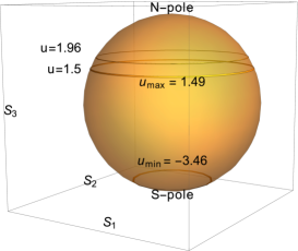
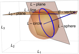
First, putting defines a -sphere (the -sphere’) in the -space as in Fig. 4.1(a). We may regard (or ) for as the latitude on the -sphere with representing the North and South poles. At each point on the -sphere, the conservation of helicity forces to lie on a plane (the -plane’) perpendicular to the numerical vector at a distance from the origin of the -space. At this point, we have assigned numerical values to and , which happen to be Casimirs of the Euclidean Poisson algebra (3.4). It remains to impose the conservation of and .
For each point on the -sphere, the condition (3.42) defines an -sphere of radius in the -space provided . Since , the conserved quantities must be chosen to satisfy . In fact, this ensures that and thus subsumes the latter. The -sphere and the -plane intersect along an -circle provided the radius of the -sphere exceeds the distance of the -plane from the origin, i.e.,
| (4.23) |
Thus, for the intersection to be nonempty, depending on the sign of , must lie below or above a particular latitude determined by (4.23). Furthermore, since , we must choose
| (4.24) |
When the inequality (4.23) is saturated, the -plane is tangent to the -sphere and the -circle shrinks to a point. In summary, the common level set of the three conserved quantities and can be viewed as a sort of fibre bundle with base given by the portion of the -sphere lying above or below a given latitude. The fibres are given by -circles of varying radii which shrink to a point along the extremal latitude.
The final conserved quantity restricts to the horizontal plane . For each nonpolar point on the -sphere, this -plane intersects the above -plane along the -line (assuming are not both zero). This line intersects the -sphere at a pair of points, provided the radius of the -sphere is greater than the distance of the -line from the origin of the -space, i.e.
| (4.25) |
The two points of intersection coincide if the inequality is saturated so that the -line is tangent to the -sphere. Note that inequality (4.25) implies (4.23), provided the -sphere is nonempty (). This is geometrically evident since the distance of the -line from the origin is bounded below by the distance of the -plane (which contains the -line) from the origin.
Remark: Another way to see that (4.25) implies (4.23) is to note that if , then
| (4.26) |
Eq. (4.25) would then imply (4.23), if we can show that on the sphere . To see this, we first note that at the poles so that it suffices to show that the quadratic polynomial is nonnegative for . This is indeed the case since the global minimum of attained at is simply zero.
Assuming (4.25) holds, the common level set of all four conserved quantities may be viewed as a sort of fibre bundle with base given by the part of the -sphere satisfying (4.25) and fibres given by either one or a pair of points (this is the case for nonpolar latitudes, see below for the special circumstance that occurs above the poles). In other words, provided , the ‘base’ space is the part of the -sphere consisting of all latitudes lying in the interval and satisfying the cubic inequality following from (4.25)
| (4.27) |
The roots of the cubic equation resulting from the saturation of this inequality determine the extremal latitudes where the two-point fibres degenerate to a single point (provided the extremal latitude does not correspond to a pole of the -sphere). If an extremal latitude is at one of the poles then must vanish there and the determination of the fibre over the pole is treated below.
Recall that the discriminant of the cubic is the product of squares of differences between its roots. It vanishes iff a pair of roots coincide. The discriminant of the cubic will be useful in the analysis that follows. It is a function of the four conserved quantities:
| (4.29) | |||||
4.1.3.2 Fibres over the poles of the -sphere
At the and poles of the -sphere, the -plane and -plane are both horizontal: their intersection does not define an -line. For the common level sets of and to be nonempty, the planes must coincide:
| (4.30) |
with upper/lower signs corresponding to the poles. This condition ensures that vanishes at the corresponding pole, implying that it cannot be positive at a physically allowed pole of the -sphere.
Now, for the -sphere to intersect the -plane, its radius must be bounded below by :
| (4.31) |
When this inequality is strict, the fibre over the pole is a circle (-circle) while it is a single point when the inequality is saturated. Interestingly, in the latter case, the discriminant (4.29) vanishes, so that the pole must either be a double or triple zero of . On the other hand, when the inequality is strict, must have a simple zero at the pole. This structure of fibres over the poles is in contrast to the two point fibres over the non polar latitudes of the -sphere when . For example, suppose and take so that the and -planes over the pole coincide. These planes intersect the -sphere provided (see (4.31)). Moreover, the fibre over the pole is a single point if and a circle if .
4.1.3.3 Properties of and the closed, connectedness of common level sets
We observed in Section 4.1.3.2 that must vanish at a physically allowed pole of the -sphere and that we must have for this to happen. Here, we investigate the possible behaviour of near a pole, which helps in restricting the allowed graphs of . We find that the sign of at an allowed pole is fixed and also that the allowed latitudes must form a closed and connected set. As a consequence, we deduce that some graphs of are disallowed. For example, cannot have a triple zero at a nonpolar latitude. We also deduce that the common level sets must be both closed and connected.
Result 1: Sign of at a pole which is a simple zero: Suppose has a simple zero at the pole with nonempty fibre over it, then .
Proof of : Suppose , so that has a simple zero at the pole with circular fibre over it (see Eq.(4.30)). Then (4.27) implies
| (4.32) |
Suppose , then . But in this case, the upper bound on the latitude so that could not have been an allowed latitude. On the other hand, if , then is an allowed latitude. Thus, when the pole for is a simple zero of with nonempty fibre, it is always surrounded by other allowed latitudes. In particular, the north poles in Fig. 4.2g, j and k are not allowed latitudes, while they are in Fig. 4.2c and h.
Proof of : On the other hand, suppose so that has a simple zero at with nonempty fibre. Suppose , then as before (4.27) implies which violates (4.24). Thus must be positive. In other words, when the pole is a simple zero of with nonempty fibre, it must be surrounded by other allowed latitudes. So the poles cannot be simple zeros unless the neighbouring latitudes are allowed. In particular, the south poles in Fig. 4.2d, h, i and j are allowed latitudes.
Result 2: Set of allowed latitudes and common level set must be closed: The conserved quantities and define continuous functions (quadratic in and ) from the phase space to the four-dimensional space of conserved quantities (which is a subset of consisting of the 4-tuples subject to the conditions and (4.24)). Each of their common level sets must be a closed subset of as it is the inverse image of a point in . We may use this to deduce that cannot approach a positive value at a pole. We have already observed that if a pole is an allowed latitude then must vanish there. On the other hand, suppose a pole is not an allowed latitude but is positive in a neighbourhood of . Then the set of allowed latitudes would be an open set and so would the common level set. In particular, cannot have (i) only one simple zero on the -sphere and be nonvanishing elsewhere (as in Fig. 4.2n) (ii) three simple zeros between the poles (see Fig. 4.2m) (iii) a double zero and a simple zero between the poles (iv) a triple zero at a nonpolar latitude (v) two simple zeros between the poles with at the poles (as in Fig. 4.2o) or (vi) a double zero between the poles with at the poles.
Common level set of conserved quantities must be connected: For the common level set to be disconnected, the set of allowed latitudes on the -sphere must be disconnected. The only remaining way that this could happen is for to have three distinct simple zeros on latitudes of the -sphere. Let us show that this is disallowed. Now Result 2 prevents from having three simple zeros at nonpolar latitudes. It only remains to consider the cases where either of the poles is a simple zero of . If has a simple zero at , then by Result 1, . Since , can have at most one more zero on the -sphere so that the set of allowed latitudes is connected. On the other hand, suppose has a simple zero at , then by Result 1. Suppose further that has two more simple zeros on the -sphere, then by Result 2, must equal as otherwise would be positive at the pole as in the disallowed Figs. 4.2m, n and o. So with as in Fig. 4.2j. But in this case, Result 1 forbids from being an allowed latitude, so that the set of allowed latitudes is again a single interval .
Triple zeros of : For (4.27) to have a triple zero, i.e., to be of the form , we must have and the conserved quantities must satisfy two conditions:
| (4.33) |
These conditions define a two-dimensional surface in the space of conserved quantities. Result 2 implies that cannot have a triple zero at a nonpolar latitude. On the other hand, can have a triple zero at or provided both (4.30) and (4.33) are satisfied. Putting in (4.33), the conditions for or to be a triple zero become
| (4.34) |
The first condition implies that cannot have a triple zero at for or at for . On the other hand, can have a triple zero at for as in Fig. 4.2l.
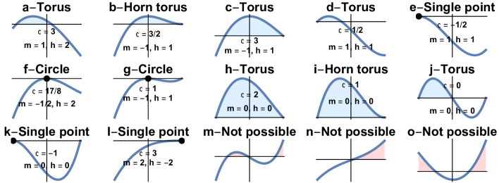
4.1.3.4 Possible types of common level sets of all four conserved quantities
Here we combine the above results on the connectedness of common level sets, slope of at the poles and on the structure of the fibres over polar and nonpolar latitudes of the -sphere to identify all possible common level sets of conserved quantities. There are only four possibilities: the degenerate or singular level sets (horn tori, circles and single points) and the generic common level sets (2-tori). These possibilities are distinguished by the location of roots of . They are discussed below and illustrated in Fig 4.2. In (C1)-(C5) below we take so that correspond to the and poles. Similar results hold for with and interchanged.
(C1) For generic values of conserved quantities, is positive between two neighbouring nonpolar simple zeros lying in (E.g. , and as in Fig. 4.2a). The base space of Section 4.1.3 is the portion of the -sphere lying between the latitudes and , with the two-point fibres shrinking to single point fibres along the extremal latitudes and . The resulting common level set is homeomorphic to a pair of finite coaxial cylinders with top as well as bottom edges identified, i.e., a -torus.
To visualize the above toroidal common level sets and some of its limiting cases which follow, it helps to qualitatively relate the separation between zeros of to the geometric parameters of the torus embedded in three dimensions. For instance, the minor diameter of the torus grows with the distance between and . Thus, when the simple zeros coalesce at a double zero, the minor diameter vanishes and the torus shrinks to a circle. Similarly (for ) the major diameter of the torus grows with the distance between and . Thus, when , the major and minor diameters become equal and we expect the torus to become a horn torus. However, this requires the fibre over to be a single point, which is true only when is a double zero of .
(C2) A limit of (C1) where either or and is positive between them. For instance, if and the fibre over is a single point, then the common level set is homeomorphic to a horn torus (E.g. , and as in Fig. 4.2b). On the other hand, for the fibre over is a circle and we expect the common level set to be a -torus (see Fig. 4.2c). It is as if the circular fibre over the single-point latitude plays the role of an extremal circular latitude with single point fibre in (C1), thus the roles of base and fibre are reversed. Similarly, when with circular fibre over , the common level set is homeomorphic to a 2-torus (E.g. and as in Fig. 4.2d). In the limiting case where , the two simple zeros and merge at . The fibre over becomes a single point and the common level shrinks to a point (see Fig. 4.2e).
(C3) Another limit of (C1) where the roots and coalesce at a double root of . is negative on the -sphere except along the latitude and the fibre over it is a single point. The discriminant (4.29) must vanish for this to happen. The common level set becomes a circle corresponding to the latitude . For example, if and and , then the equator is the allowed latitude as shown in Fig. 4.2f. Another example of a circular common level set appears in Fig. 4.2g. In this case Results 1 and 2 exclude the north pole ensuring the connectedness of the common level set.
(C4) A limit of (C1) where the simple zeros and move to and respectively, with in between. In this case, both poles have circular fibres and the common level set is a 2-torus. This happens, for instance, when , irrespective of the values of and . Another way for this to happen is for and to vanish so that the poles are automatically zeros of
| (4.35) |
and to choose to ensure there is no zero in between. Holding and fixed, three more possibilities arise as we decrease . When , has a double zero at (Fig. 4.2i) with a single point fibre over it and the common level set becomes a horn torus. For , the third zero of moves from to the latitude . By Result 1, the allowed latitudes go from to (see Fig. 4.2j), and the common level set returns to being a -torus. Finally, when , the only allowed latitude is a double zero and the common level set shrinks to a point (see Fig. 4.2k).
(C5) has a zero at just one of the poles and is negative elsewhere on the -sphere. The common level set is then a single point. We encountered this as a limiting case of (C2) where has a double zero at as in Fig. 4.2e. This can also happen when is negative on the -sphere except for a triple zero at either () or () (see Eq. (4.34)). For example, when , and , has a triple zero at as in Fig. 4.2l.
4.1.4 Nature of the ‘Hill’ region and energy level sets using Morse theory
In this section, we study the ‘Hill’ region , which we define as the set of points on the symplectic leaf with energy less than or equal to :
| (4.36) |
The energy level set is then the boundary of . Taking and (4.6) as coordinates on , we treat the Hamiltonian
| (4.37) |
as a Morse function [49]. The nature of critical points of depends on the value of . There are two types of critical points: (a) an isolated critical point at which exists for all values of and (b) a ring of critical points
| (4.38) |
which exists only for and shrinks to the isolated critical point when . The energy at these critical points is
| (4.39) |
Upon varying and , the isolated critical points cover all of the static submanifold while the rings of critical points cover the static submanifold . By finding the eigenvalues of the Hessian of the Hamiltonian at these critical points, we find that for the isolated critical point G is a local minimum of energy (four +ve eigenvalues). In fact, for , the isolated critical point has to be the global minimum of energy as the energy is bounded below and there are no other extrema of energy. For , the isolated critical point becomes a saddle point (two +ve and two -ve eigenvalues) with energy . On the other hand, the ring of critical points are degenerate global minima (three +ve and one zero eigenvalue). To apply Morse theory, we need the indices of the critical points of (number of negative eigenvalues of the Hessian). From the foregoing, we see that the ground state G has index zero, the saddle point has index two and the degenerate critical points on the ring may be nominally assigned a vanishing index.
Change in topology of the Hill region: According to Morse theory [49], the topology of the Hill region can change only at critical points of the Hamiltonian. (a) For , there is only one critical point, the global minimum G with index zero and energy . Thus, as increases beyond , the Hill region goes from being empty to being homeomorphic to a 4-ball arising from the addition of a 0-cell. (b) For , there are two critical values of energy corresponding to the ring of critical points and the saddle point. The index vanishes along the ring of critical points, so when crosses , the Hill region acquires a 3-ball (0-cell) for each point on the ring corresponding to the 3 positive eigenvalues of the Hessian. Thus for . The saddle point with has index two, so the topology of changes to upon adding a 2-cell to (the analogous statement in one lower dimension is that adding a 2-cell to the hole of the solid torus gives a ).
Nature of energy level sets: The energy level set is the boundary of the Hill region, i.e. . It is a 3-manifold except possibly at the critical energies. Thus for , for all energies . On the other hand, when the energy level set undergoes a change in topology from to as crosses .
The energy level sets at the critical values and are exceptional. For given and with and , is a single point on (the critical point), since G is the nondegenerate global minimum of energy. When , fixes leaving a range of possible values of , whose values are determined by eliminating from the conditions . This leads to a three-dimensional energy level set. includes one horn torus with its center as the saddle point for as well as a one parameter family of toroidal level sets for and a pair of circular level sets occurring at and . Interestingly, horn tori arise only when , since is a necessary condition for horn tori (see Section 4.2.2). Thus, the horn torus is a bit like the figure-8 shaped separatrix one encounters in particle motion in a double well potential. Finally, the level manifold consists of a ring of single point common level sets, each lying on the static submanifold . Unlike static solutions and horn tori, circular and 2-toroidal level sets also arise at noncritical energies.
4.2 Foliation of phase space by tori, horn tori, circles and points
For generic allowed values of the conserved quantities and , their common level set in the phase space is a -torus. As noted, this happens when has simple zeros along a pair of latitudes of the -sphere and is positive between them. However, this -parameter family of invariant tori does not completely foliate the phase space: there are some other ‘singular’ level sets as well: horn tori, circles and points. The union of single-point level sets is (4.5), consisting of static solutions. They occur when has a triple zero at or is a local maximum at a double zero at . We will now discuss the other cases in increasing order of complexity. In each case, we view the union of common level sets of a given type as the state space of a self-contained dynamical system which has the structure of a fibre bundle over an appropriate submanifold of the space of conserved quantities. The fibres in each case are circles, horn tori and tori. The dynamics on the union of circles and tori is Hamiltonian and we identify action-angle variables on them. On the other hand, we show that the dynamics on the union of horn tori is a gradient flow.
4.2.1 Union of circular level sets: Poisson structure & action-angle variables
In this section, we show that the union of circular level sets is the same as the trigonometric/circular submanifold (introduced in Section 3.2.5) where the solutions are sinusoidal functions of time. Local coordinates on are furnished by and (or equivalently ) and we express the Hamiltonian in terms of them. The Poisson structure on is degenerate with and generating the center and their common level sets being the symplectic leaves. While is a constant of motion, evolves linearly in time. We exploit these features to obtain a set of action-angle variables for the dynamics on .
4.2.1.1 as a circle bundle and dynamics on it
As pointed out in example (C3) of Section 4.1.3.4, the common level set of conserved quantities is a circle when the cubic (4.27) has a double zero at a nonpolar latitude of the -sphere and is negative on either side of it. In this case, the latitude is restricted to the location of the double zero. To identify the three-dimensional hypersurface in the four-dimensional space of conserved quantities, where has a double zero at a nonpolar latitude, we will proceed in two steps. First, we compare the equation with to arrive at the three conditions:
| (4.40) |
The first two may be used to express the roots and in terms of conserved quantities:
| (4.41) |
The third equation in (4.40) then leads to the following conditions among conserved quantities
| (4.42) |
Squaring, these conditions are equivalent to , where is the discriminant (4.29) of . The three-dimensional submanifold of defined by , however, includes 4-tuples (, , , ) corresponding to horn toroidal (double zero at the pole ) or single-point (triple zero at or double zero at or ) common level sets, in addition to circular level sets. To eliminate the former, we must impose the further conditions , and . This last condition, which says , selects the roots in (4.41). These conditions define the three-dimensional hypersurface corresponding to circular level sets. Now, and may be chosen as coordinates on , with (4.42) allowing us to express in terms of them. Interestingly, we find by studying examples, that for values of and corresponding to a circular level set, there are generically two distinct values of ; so we would need two such coordinate patches to cover . The union of all these circular level sets may be viewed as a sort of circle bundle over and forms a four-dimensional ‘circular’ submanifold of . As shown in Section 3.2.5 and Section 3.2.6, this circular submanifold along with its boundary coincides with the set where the four-fold wedge product vanishes.
The equations of motion (2.29) simplify on the circular submanifold . Indeed, since is a constant, so that implying that where . As shown in Section 3.2.5, the equations of motion then simplify to
| (4.43) |
with sinusoidal solutions:
| (4.44) |
Here, using (2.32), , which varies with location on the base . It is the nondimensional angular velocity for motion in the circular fibres. Since and are positive, . Here both and evolve linearly in time and the equality of
| (4.45) |
implies that the constant of motion may be expressed in terms of and :
| (4.46) |
Remark: If the -sphere shrinks to a point then one still has circular level sets consisting of latitudes of the -sphere determined by , provided . However, each point on these exceptional circular level sets is a static solution lying on (4.5).
4.2.1.2 Canonical coordinates on
Local coordinates on : For the analysis that follows, a convenient set of coordinates on the ‘circle bundle’ consists of and for the base and for the fibres. The dynamics on admits three independent conserved quantities as there is one relation among and following from (4.42). Since the common level sets of the conserved quantities on are circles, rather than tori, it is reasonable to expect there to be two Casimirs (say and ) for the Poisson structure on , as we show below. In fact, is foliated by the common level surfaces of and (symplectic leaves) which serve as phase spaces (with coordinates and ) for a system with one degree of freedom. is then the coordinate along the circular level sets of the Hamiltonian on these two-dimensional symplectic leaves.
To find the reduced Hamiltonian on we express the remaining variables in terms of and . The formula for (3.42) along with (4.46) determines and consequently as well. The remaining conserved quantities are given by
| (4.47) | |||||
| (4.48) |
Thus, the reduction of the Hamiltonian (3.1) to the trigonometric submanifold is
| (4.49) |
As remarked, for given values of and , there are generically two possible values of corresponding to two points on . By considering examples, we verified that for each of them, there is a unique that satisfies (4.46) and both the equations in (4.48).
Poisson structure on : We wish to identify Poisson brackets among the coordinates and that along with the reduced Hamiltonian (4.49) gives the equation of motion on . As noted, it is natural to take and as Casimirs so that . The only nontrivial Poisson bracket is then determined as follows from (4.49):
| (4.50) |
Moreover, this implies , which notably differs from the original nilpotent Poisson bracket (3.2).
Canonical action-angle variables on : Since evolves linearly in time, it is a natural candidate for an angle variable. The corresponding canonically conjugate action variable must be a function of and and is determined from (4.50) by the condition . We thus obtain, up to an additive constant, the action variable
| (4.51) |
Thus we arrive at the remarkably simple conclusion that (aside from the Casimirs and ) and are action-angle variables on . Moreover, the canonical Poisson bracket agrees with that on the full phase space (see (4.73)). Our reason to work with rather than as a coordinate is that the solutions (4.44) and the Hamiltonian (4.49) have simple expressions in terms of . By solving the cubic (4.51), can be expressed in terms of , which would allow us to write the Hamiltonian in terms of the action variable .
4.2.2 Union of horn toroidal level sets: Dynamics as gradient flow
Just as with the union of circular level sets , the union of horn toroidal level sets serves as the phase space for a self-contained dynamical system. However, unlike the sinusoidal periodic trajectories on , all solutions on are hyperbolic functions of time and are in fact homoclinic orbits joining the center of a horn torus to itself (see Fig. 4.3). The centers themselves are static solutions. Horn tori arise only when the energy is equal to the critical value given in Section 4.1.4. Thus, the horn tori are like the figure-8 shaped separatrices in the problem of a particle in a double well potential, separating two families of 2-tori. Interestingly, though the conserved quantities satisfy a relation on each horn torus, the four-fold wedge product vanishes only at its center. Finally, unlike on the circular submanifold, the flow on the horn-toroidal submanifold is not Hamiltonian, though we are able express it as a gradient flow.
The family of horn toroidal level sets is a two-dimensional submanifold of the four-dimensional space of conserved quantities . To see this, note that a horn torus arises when the cubic of (4.27) is positive between a simple zero and a double zero at the pole of the -sphere. Thus, must be of the form where with . These requirements imply and . Note that each nontrivial horn torus is a smooth two-dimensional surface except at its center which lies at the pole . Trivial horn tori are those that have shrunk to the points at their centers and arise when . The conditions and lead to two relations among conserved quantities
| (4.52) |
which together imply that . The inequality along with (4.52) restricts us to points above a parabola in the - plane:
| (4.53) |
The space is given by the set of such pairs. For each we get a horn torus . The union of all horn tori is then given by .
4.2.2.1 as a four-dimensional submanifold of
Equations (4.52) and (4.53) when expressed in terms of and allow us to view the union of all horn tori as a four-dimensional submanifold of :
| (4.54) |
For any choice of , the first two conditions define a plane through the origin (normal to ) and a cylinder (of radius with axis along ) in the -space. In general, this plane and cylinder intersect along an ellipse so that may be viewed as a kind of ellipse bundle over the -space (subject to the inequality). The centers of the horn tori are the points where , and (see Section 4.2.2.2 below). Interestingly, it turns out that the inequality in (4.54) restricting the range of is automatically satisfied at all points of the base space other than when (which correspond to centers of horn tori). Indeed, let us find the range of values of allowed by the first two relations in (4.54) by parameterizing the elliptical fibre by the cylindrical coordinate . Then , and . The extremal values of on the ellipse occur at which implies that
| (4.55) |
Thus the inequality in (4.54) is automatically satisfied away from the axis which corresponds to the centers of horn tori.
4.2.2.2 Centers of horn tori and punctured horn tori
It turns out that the centers of horn tori are static solutions and may therefore be regarded as forming the boundary of . In particular, a trajectory on a horn torus can reach its center only when . To find the space of centers we note that they lie at the pole corresponding to and . The conditions (4.54) then become
| (4.56) |
The first condition is automatic, the second implies while the inequality becomes . Thus is the two-dimensional subset of the static submanifold consisting of points on the - plane, on or within the parabola . The points on the parabola correspond to trivial horn tori. By eliminating their centers we obtain (nontrivial) punctured horn tori which are smooth noncompact surfaces with the topology of infinite cylinders on which the dynamics is everywhere non static. We let denote the four-dimensional space consisting of the union of punctured horn tori. Thus may be regarded as a cylinder bundle over the base . Some possible coordinates on are (a) (b) and (c) and either or .
4.2.2.3 Nonvanishing four-fold wedge product on
We have argued that the conserved quantities satisfy the relations (4.52) on . Despite this, we show that the wedge product does not vanish on except on its boundary . To see this, note that in addition to the condition (due to the presence of the double zero at the pole ), all four partial derivatives of may be shown to vanish on by virtue (4.52). In other words, the relation following from is vacuous on (if not, we could wedge it, say, with to show that ). On the other hand, we showed in Section 3.2.6 that vanishes precisely on the closure of the circular submanifold . Thus, to show that is nonvanishing on , it suffices to find the points common to and . Now is empty as has a double/triple zero at for points on and a double zero away from the poles for points on . In fact, we find that is contained in the static submanifold so that is nowhere zero on and vanishes only on its boundary . To see that does not have any points in common with either or we observe that the conditions , (4.52) and the relations ( and ) or ( and ) that go into the definitions of and or (see Section 3.2.6), together define a parabola in phase space
| (4.57) |
This parabola is contained in but does not lie on or as the inequalities and appearing in the definitions of and are saturated along it. Points on this parabola correspond to horn tori that have shrunk to the single point at their centers and correspond to cubics with a triple zero at . Thus, this parabola lies along the common boundary of and . Combining these results we see that on , but vanishes identically on its boundary consisting of the space of centers .
4.2.2.4 Equations of motion on the horn torus:
On the horn torus the evolution equation for (4.13) simplifies:
| (4.58) |
We may interpret this equation as describing the zero energy trajectory of a nonrelativistic particle of mass 2 with position moving in a one-dimensional potential . Since is negative between the simple and double zeros at and , the former is a turning point while the particle takes infinitely long to reach/emerge from . Thus, the trajectory is like a solitary wave of depression. Choosing to be its minimal value , the trajectory of the particle is given by
| (4.59) |
Notice that as , and the solution approaches the center of the horn torus. Interestingly, the vector field is not smooth at , which is a square root branch point. Thus, there is another solution with the same initial condition (IC) , which however is consistent with the - equations of motion (2.29) only when . Note that (4.59) can be obtained as a limit of the -function solution given in Section 4.1.2. On a horn torus, one of the half periods of the -function is imaginary while the other diverges leading to the aperiodic solution (4.59).
To describe the trajectories on a horn torus we use the coordinates and in terms of which the equations of motion (3.52) simplify to
| (4.60) |
Notice that is monotonic in time: increasing/decreasing according as . It is convenient to pick ICs on the curve resulting in the solution
| (4.61) |
Though and are both ill-defined at the center of the horn torus (), we notice from (3.50) that the difference is well defined at the center:
| (4.62) |
Since is ill-defined at the center , it is convenient to switch to the ‘embedding’ variables:
| (4.63) |
The advantage of is that it approaches as on any trajectory on . We may visualize the dynamics via the following embedding of the horn torus in Euclidean 3-space:
| (4.64) |
Here is the major (as well as the minor) radius of the horn torus (see Fig. 4.3(a)). Alternatively, we may realize the punctured horn torus as a cylinder in three-dimensional space via the embedding
| (4.65) |
The center of the horn torus lies at with arbitrary (see Fig. 4.3(b)). As all trajectories spiral into the center of the horn torus as shown in Fig. 4.3. Thus, every trajectory is homoclinic, beginning and ending at the center of the horn torus.
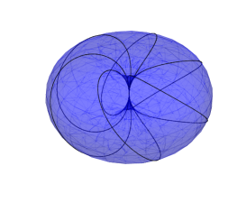
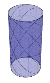
As noted in Section 4.1.4, horn tori arise only at the saddle points of the Hamiltonian . Thus, they are analogs of the figure-8 shaped separatrix at energy familiar from particle motion in the one-dimensional potential . For fixed with , and , can take a range of values from to . There is a critical value in this range at which the common level set is a horn torus. It is flanked by 2-tori on either side. Thus, horn tori separate two families of toroidal level sets with the real half-period of the -function diverging as .
4.2.2.5 Flow on is not Hamiltonian
The equations of motion on
| (4.66) |
do not follow from any Hamiltonian and Poisson brackets on . This is because time-evolution does not satisfy the Liouville property of preserving phase volume: every initial condition is attracted to the center of a horn torus. Said differently, the flow can map a subset of into a proper subset . To show this, it suffices to consider the dynamics on each separately since the dynamics preserves individual punctured horn tori. Thus, consider the ‘upper cylinder’ subset of : . Then
| (4.67) |
is its image under evolution to time . Since is monotonic in time, we observe that for , form a 1-parameter family of subsets with decreasing volume (relative to any reasonable volume measure on ) while grows if . Thus, the Liouville theorem would be violated if the dynamics on or were Hamiltonian.
Interestingly, time evolution on may be realized as a gradient flow. As before, we focus on the dynamics on each separately. Since is monotonically decreasing in time (4.66), we choose it as the potential function for the gradient flow
| (4.68) |
The inverse-metric on that leads to this gradient flow must be of the form
| (4.69) |
Here is an arbitrary function on which we may choose so that the metric is, for simplicity, Riemannian (positive definite). This is ensured if
| (4.70) |
The second condition is implied by the first, so a simple choice that ensures a Riemannian metric is , for any . It might come as a surprise that this gradient flow admits homoclinic orbits beginning and ending at the center. Such orbits are typically forbidden in gradient flows. Our horn tori evade this ‘no-go theorem’ since the potential is not defined at the centers of horn tori.
4.2.3 Dynamics on the union of toroidal level sets
For generic values of and , i.e., for which the discriminant (4.29), the common level sets are 2-tori as shown in Section 4.1.2.1 and Section 4.1.3. The union of these 2-tori may be viewed as the state space of a self-contained dynamical system. Here, we express as a torus bundle over a space of conserved quantities, and find a convenient set of local coordinates on it along with their Poisson brackets implied by (3.2). We use this Poisson structure and the time evolution of in terms of the function (4.16) to find a family of action-angle variables on . Finally, we show that these action-angle variables degenerate to those on the union of circular level sets when the tori degenerate to circles.
4.2.3.1 Union of toroidal level sets
Let us denote by , the subset of the space of conserved quantities for which the common level sets are 2-tori. On the cubic (4.27) is positive between two adjacent simple zeros and and the common level set is a torus. Thus, on the cubic takes the form with and . In this case, when is written in Weierstrass normal form using , the invariants and are real and the discriminant of the cubic is nonzero. It follows that the half periods and of Section 4.1.2 are respectively real and purely imaginary. We designate the union of these tori and the corresponding union for fixed and , . Here, may be visualised as a torus bundle over . While and furnish global coordinates on the torus , it is more convenient, when formulating the dynamics, to work with the local coordinates where . An advantage of is that unlike , it commutes with . However, since the cosine is a 2:1 function on , we need two patches with local coordinates to cover the torus with and . In the patches, the formula for is
| (4.71) |
where the function is defined to take values between and . Whenever reaches either or , the trajectory crosses over from one patch to the other.
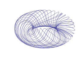
4.2.3.2 Poisson structure on
On , we use the local coordinates and . The Poisson structure following from the nilpotent Poisson brackets (3.2) is degenerate with the Casimirs and generating the center. The Poisson brackets among the remaining coordinates (on ) are:
| (4.72) | |||||
| (4.73) |
All the Poisson brackets other than have a common expression on both patches . Here and .
4.2.3.3 Action-angle variables on
We seek angle-action variables on satisfying canonical Poisson brackets
| (4.74) |
The action variables and must be conserved and therefore functions of and alone, while the angles and must evolve linearly in time: . Here we suppress the parametric dependence of and on the Casimirs and which specify the symplectic leaf. In what follows, we use the -function solution (4.16) along with the requirement of canonical Poisson brackets to find a family of action-angle variables. Despite some long expressions in the intermediate steps, the final formulae (4.99) for are relatively compact. Though we work here with the nilpotent Poisson structure (4.73), it should be possible to generalize the resulting action-angle variables to the other members of the Poisson pencil (3.11).
Determination of and : The evolution of (4.16) gives us one candidate for an angle variable evolving linearly in time
| (4.75) |
The factor of is chosen to make dimensionless. Here, and (4.15) are functions of the conserved quantities. From the definition of , it follows that the frequency . Choosing to be the imaginary half-period of the -function in (4.16) ensures that is real. An action variable conjugate to is
| (4.76) |
where is an arbitrary function of (and possibly and ) to be fixed later. Upto the function , is proportional to the Hamiltonian (3.43). Eq. (4.76) is obtained by requiring
| (4.77) |
Here, (see Section 4.1.2) and we used the relation
| (4.78) |
For future reference we also note that as a consequence, . This derivative diverges at and , which are the roots of .
Determination of and : To identify the remaining action-angle variables and we first consider the constraints coming from the requirement that their Poisson brackets be canonical. While is automatic, implies that must be independent of :
| (4.79) |
The remaining Poisson brackets help to constrain . For instance, forces to be a linear function of :
| (4.80) |
Here is an arbitrary function which we will now try to determine. Next, implies that evolves linearly in time:
| (4.81) | |||||
| (4.82) |
Comparing (4.80) and (4.82), it follows that is independent of . We may use (4.82) to reduce the determination of the dependence of on to quadratures:
| (4.83) |
Using (3.52) and (4.13) we get
| (4.84) |
Integrating,
| (4.85) |
where . Recognizing these as incomplete elliptic integrals of the first and third kinds ( and ), we get (see Section 3.131, Eq. (3) and Section 3.137, Eq. (3) of [31])
| (4.86) |
Here, is an integration constant, where (which are functions of and ) are the roots of the cubic . Moreover, the amplitude and elliptic modulus are
| (4.87) |
To find the dependence of , we notice that the last Poisson bracket gives the following relation among derivatives of :
| (4.88) | |||||
| (4.89) |
Using the known formulae for the partial derivatives (4.75, 4.78, 4.82, 4.83)
| (4.90) |
we find the dependence of from (4.89):
| (4.91) |
In effect, we have two expressions ((4.86) and (4.91)) for . We exploit them to reduce the determination of the dependence of to quadrature. Comparing (4.86) with (4.91) gives
| (4.93) | |||||
Thus
| (4.95) | |||||
Here is an arbitrary ‘constant’ of integration. Now, using (4.95) in (4.86) results in some pleasant cancellations leading to a relatively simple formula for :
| (4.96) |
This determines the angle variable . It is noteworthy that is simply . The integral over is from since, for sufficiently large , (4.29) is always positive so that is a torus. However, we must take , which is the value at which vanishes and the torus shrinks to a circle.
Remark: Consistency requires that the RHS of (4.95) be independent of , which enters through and . We verify this by showing that (4.96) agrees with (4.84). In fact, from (4.96) and using and (4.27),
| (4.97) |
which agrees with (4.84). As (4.27) is a quadratic function of , the integrand behaves as for large , so that the lower limit does not contribute.
Summary: Thus, aside from the Casimirs and , the action-angle variables on the union of toroidal level sets are given by the following functions of , , and :
| (4.98) | |||||
| (4.99) |
We have verified by explicit calculation that these variables are canonically conjugate. As a function of , increases from zero to (4.16). As noted, depends linearly on , but finding its dependence on and requires the evaluation of the integral over in (4.99). We have not been able to do this analytically but could evaluate it numerically for given and . Here, and are arbitrary functions of , with and nonzero and the frequency . A simple choice is to take
| (4.100) |
For this choice, the Hamiltonian (3.43) acquires a simple form in terms of the action variables
| (4.101) |
The corresponding frequencies are then both equal to . Though the frequencies are equal, the periodic coordinates and generally have different and incommensurate ranges, so that the trajectories are quasi-periodic (see Fig. 4.4). While we do not have a simple formula for the range of , that of is (twice its increment as goes from to , see Eq. (4.16)), which depends on the symplectic leaf and invariant torus via the four conserved quantities.
Relation to action-angle variables on the circular submanifold: Finally, we show how the action-angle variables obtained above degenerate to those on the circular submanifold of Section 4.2.1, where the elliptic function solutions reduce to trigonometric functions with the imaginary half-period diverging. For given and , we must let to reach the circular submanifold. On , the simple zeros of , and coalesce at a double zero so that becomes a constant. Thus, the angle variable (4.99) ceases to be dynamical. In the same limit, from (4.99), the surviving angle variable becomes a linear function of with constant coefficients. Moreover, for the simple choices of Eq. (4.100), we get and upto an additive constant. Pleasantly, these action-angle variables are seen to agree with those obtained earlier on (4.51).
Chapter 5 Quantum Rajeev-Ranken model as an anharmonic oscillator
In this Chapter, which is based on [44], we discuss some aspects of the quantum version of the Rajeev-Ranken model. We begin with Rajeev and Ranken’s mechanical interpretation of the model in terms of a charged particle moving in an electromagnetic field and its quantization. We find an error in their calculation of the effective potential seen by the particle which unfortunately affect their results on the spectrum and strong coupling dispersion relation. We derive the corrected effective potential in Section 5.1 and to be doubly sure we also take a complementary approach by interpreting the RR model as a quartic oscillator. Using this new mechanical interpretation we canonically quantize the model and separate variables in the Schrödinger equation. Its radial equation is shown to be an ODE of type (in Ince’s classification, see Appendix E, Section E.4), which may be regarded as a generalization of the Lamé equation. We analyze a weak and a novel strong coupling limit of the radial equation to obtain dispersion relations for the corresponding quantized screw-type waves. In another direction, we interpret the EOM of the RR model as Euler equations for a step-3 nilpotent algebra and exploit our canonical quantization to find a unitary representation of this algebra.
5.1 Electromagnetic interpretation of the RR model
Before interpreting the RR model as an anharmonic oscillator, we revisit the mechanical interpretation given by Rajeev and Ranken in terms of a charged particle moving in a static electromagnetic field. Here, we implement this general idea and derive the classical and quantum equations of motions. In the process, we notice certain errors in the analysis of Rajeev and Ranken, which affect their results on the spectrum and dispersion relations. This unfortunately cast doubts on their results.
The Hamiltonian of the RR model in Darboux coordinates for is:
| (5.1) |
Suppose the Cartesian position and momentum coordinates of a charged particle are
| (5.2) |
then the Hamiltonian in (5.1) can be rewritten as:
| (5.3) |
in units where the charged particle has mass , charge and the speed of light . This describes a charged particle moving in an EM field arising from the vector and scalar potentials:
| (5.4) | |||||
| (5.5) |
The corresponding electromagnetic field is axisymmetric with pointing radially inward and having both azimuthal and axial components:
| (5.6) |
The Hamiltonian in (5.3) along with the canonical PBs gives the Newton-Lorentz equations . In fact, using
| (5.7) |
we get the NL equations in component form
| (5.8) | |||||
| (5.9) |
These are seen to agree with (2.36) in units where upon use of (5.2).
5.1.1 Classical Hamiltonian in terms of cylindrical coordinates
The Hamiltonian (5.3) is invariant under rotation about and translation along the -axis, so we make a canonical transformation to cylindrical coordinates , and and their momenta , and satisfying the PBs
| (5.10) |
The Hamiltonian corresponding to (5.3) is [58]
| (5.11) |
where the scalar and the magnetic vector potentials are
| (5.12) |
The resulting electric and magnetic fields are
| (5.13) |
In terms of velocities the canonical conjugate momenta are
| (5.14) |
Note that and are not simply the components. In terms of these coordinates (5.9) become
| (5.15) |
5.1.2 Quantization of the electromagnetic Hamiltonian
To quantize in Cartesian coordinates we represent the canonical momenta by the differential operators:
| (5.16) |
satisfying the canonical commutation relations . The Hamiltonian (5.3) becomes the operator
| (5.18) | |||||
To facilitate separation of variables, we transform to cylindrical coordinates using
| (5.19) |
Thus we have
| (5.22) | |||||
Similarly,
| (5.25) | |||||
Adding these terms, we get
| (5.26) | |||||
| (5.27) | |||||
| (5.28) |
Thus, the Hamiltonian in cylindrical coordinates is:
| (5.29) |
where
| (5.30) |
If we introduce the momentum operators [47]
| (5.31) |
which furnish a representation of the canonical commutation relations and are hermitian with respect to the inner product , then the Hamiltonian (5.29) may be written as111 Here, (5.32) :
| (5.33) |
We note that this Hamiltonian differs from the direct quantization of the classical cylindrical Hamiltonian (5.11) by a centripetal potential . Thus, we choose to define the quantum theory via the canonical quantization in Cartesian coordinates.
We can separate variables in the Schrödinger equation using the symmetries of (5.33). The potentials , and are independent of and so that commutes with the momentum and angular momentum . Thus and can be chosen to have common eigenstates. Consequently, the and -dependence of the energy eigenfunctions can be taken to be and , where must be an integer on account of the -periodicity of and a real number. This leads to the separation of variables in the wavefunciton:
| (5.34) |
Putting we get the radial eigenvalue problem
| (5.35) |
The prefactor in (5.34) eliminates the arises from the operator . Here, the effective potential
| (5.36) | |||||
| (5.38) | |||||
includes centrifugal (inverse-square), quadratic and quartic terms in . The ‘centrifugal’ term is attractive only when .
This effective potential (in units where ) differs from that obtained by Rajeev and Ranken (in Eq. 4.8 of [58]). More precisely, in the expression for obtained by Rajeev and Ranken, the quantity was wrongly taken as instead of . Thus, the corresponding radial equation they obtained in the strong coupling limit and the subsequent analysis to obtain the dispersion relation for quantized screw-type waves needs to be reconsidered. They proposed that the resulting dispersion relation should give a glimpse of the nature of the degrees of freedom of the scalar field theory in the strongly coupled high-energy limit. In addition, they suggested that the strong coupling limit of the scalar field theory could also be interpreted as a ‘slow-light’ post-relativistic regime. However, as we point out in Section 2.1 (also see [39]), the ‘slow-light’ limit () holding fixed is not quite the same as the strong-coupling limit of the scalar field theory.
To be doubly sure about the formula (5.38) for the effective potential in the quantum theory, we re-derive (5.35) and (5.38) through a complementary viewpoint, where the RR model is interpreted as a quartic oscillator. This simple interpretation of the RR model will facilitate our analysis of its quantum theory.
5.2 Rajeev-Ranken model as a quartic oscillator
It is possible to interpret the classical Hamiltonian of the Rajeev-Ranken model expressed in Darboux coordinates (see Eqs. (5.1, 3.20))
| (5.40) | |||||
as the Hamiltonian for a particle of mass , moving in a cylindrically symmetric quadratic plus quartic potential. To see this, we regard the Darboux coordinates and conjugate momenta as the Cartesian components of the position and conjugate momentum of a particle of mass . Using this interpretation we rewrite Eq. (5.40) as a Hamiltonian for a quartic oscillator:
| (5.42) | |||||
The second term in is proportional to the -component of angular momentum (). As mentioned in the previous section, the Hamiltonian possesses a translational symmetry along and rotation symmetry about the -axis. Thus, we make a canonical transformation to cylindrical coordinates and their conjugate momenta defined in Section 5.1.1, which satisfy the Poisson brackets (5.10). Upon doing so, the Hamiltonian (5.42) becomes
| (5.43) |
Though the terms linear in and are not conventionally present in an anharmonic oscillator Hamiltonian, the RR model requires them. Notice that, when , reduces to the Hamiltonian of a free particle, while for it is a cylindrically symmetric harmonic oscillator.
Remark: Interestingly, the Hamiltonian of a quartic anharmonic oscillator
| (5.44) |
can be re-expressed as a quadratic Hamiltonian by introducing the new variable
| (5.45) |
However, in contrast to the step-2 nilpotent - Heisenberg algebra, the new variables satisfy a step-3 nilpotent algebra (see Section 2.1 for the definition of step in a nilpotent algebra):
| (5.46) |
Similarly, introducing and , we rewrite (5.42) as a quadratic Hamiltonian:
| (5.48) | |||||
The EOM follow from this quadratic form on the step-3 nilpotent algebra:
| (5.49) | |||||
| (5.50) |
This is similar to the formulation of the RR model in terms of the variables and , where the Hamiltonian (5.123) is a quadratic form on a step-3 nilpotent Lie algebra. In this sense, the RR model joins the harmonic and anharmonic oscillators, Maxwell and Yang-Mills theory in their formulation in terms of quadratic Hamiltonians on nilpotent Lie algebras. As mentioned in [58], this formulation may facilitate finding the spectrum of the Hamiltonian using the representation theory of the underlying nilpotent group [38].
Dimensional analysis: Requiring that and have dimensions of energy, momentum and length, we find that the parameters in (5.42) have the following dimensions222However, this assignment of dimensions differs from that in the RR model [58] where are dimensionless while (5.51) :
| (5.52) |
In particular in the classical theory, is the only independent dimensionless combination and defines a nondimesional coupling constant. Since and are conserved quantities, from the structure of (5.42), the energy of any classical state can be expressed as
| (5.53) |
for some function of the three dimensionless variables and . Here, has dimensions of energy.
5.3 Quantum Rajeev-Ranken model
In this section, we study the quantum RR model by canonically quantizing the isotropic anharmonic oscillator. Quantum anharmonic oscillators have been studied in various contexts and several results have been obtained in the literature. For instance, the Schrödinger eigenvalue problem for the 1D quartic oscillator may be reduced [20] to the triconfluent Heun equation ( in Ince’s classification, see Appendix E). The energy levels of this oscillator display remarkable analytic properties in the complex coupling constant plane [13]. Some exact results are available for the -dimensional isotropic sextic oscillator [24], but they do not extend to the quartic version. Hill determinants have been used to numerically obtain the spectrum of 1D anharmonic oscillators [14] as well as 2D isotropic quartic oscillator by truncating a Frobenius series expansion [60]. However, we are not aware of any exact results for the latter system. Here, we examine the analytic properties of the Schrödinger eigenvalue problem that follows from treating the RR model as a 3D quartic oscillator and its weak and strong coupling limits.
Even before formally quantizing the RR model, we may infer the possible dependence of energy eigenvalues on parameters from dimensional analysis. From (5.52), since has dimensions of action, in the quantum theory is a second independent dimensionless combination in addition to the classically present dimensionless coupling constant . Thus, generalizing (5.53), the energy of any quantum state must be of the form
| (5.54) |
for some function of the four dimensionless combinations and .
Canonical quantization: To quantize the system in Cartesian coordinates we represent the canonical momenta as differential operators:
| (5.55) |
those satisfying the canonical commutation relations . Thus the Hamiltonian (5.42) becomes the operator
| (5.57) | |||||
To facilitate separation of variables in the Schrödinger equation, we introduce cylindrical coordinates and the corresponding momentum operators [32, 47]
| (5.58) |
which furnish a representation of the canonical commutation relations . They are hermitian with respect to the inner product . The Hamiltonian (5.57) then becomes:
| (5.59) |
Notably, this Hamiltonian differs from the direct quantization of the classical cylindrical Hamiltonian (5.43) by the addition of an attractive quantum ‘anti-centrifugal’ potential energy [16] which cancels a similar term in .
The Hamiltonian (5.59) commutes with and , so that all three operators can be chosen to have common eigenstates. Hence, the - and -dependence of the energy eigenfunctions can be taken to be and leading to the eigenfunction:
| (5.60) |
Here, can be any real number while , where must be an integer on account of the -periodicity of . Separating variables in , we arrive at a radial eigenvalue problem
| (5.61) |
with the potential333Instead if we use the wave function (5.34), then this potential agrees (in units ) with the effective potential (5.38) obtained using the electromagnetic interpretation of Section 5.1. This confirms that the effective potential in [58] has an error.
| (5.62) |
For the free particle case (), the potential is absent and (5.61) reduces to the Bessel equation [12]. In this case, is simply the energy eigenvalue of the free particle in the - plane (see Eq. (5.57)), so it must be irrespective of the value of .
It is convenient to separate out the free particle motion in the -direction and define the 2D isotropic anharmonic oscillator Hamiltonian
| (5.63) |
with eigenvalue
| (5.64) |
We notice that the coefficient of the quartic term in (5.62) is positive () while that of the quadratic term () can have either sign. Thus the potential is either purely convex or shaped like a Mexican-hat444However, the minima of the potential are not static solutions because of the term in the Hamiltonian. See Appendix F.. In either case, the spectrum of is bounded below and discrete.
5.3.1 Quantum RR model in terms of dimensionless variables
Assuming ( corresponds to a free particle), we may re-write the Hamiltonian (5.57) in terms of the dimensionless variables:
| (5.65) | |||||
| (5.66) |
Dividing (5.57) by we get the dimensionless Hamiltonian
| (5.67) |
Here . Similarly, the cylindrical coordinate Hamiltonian (5.59) may be written in terms of dimensionless variables ():
| (5.68) |
The formulation in terms of dimensionless couplings will facilitate taking strong and weak coupling limits in Section 5.3.2.
As before, using the symmetries of the Hamiltonian we separate variables in the energy eigenvalue problem (where ) for the wavefunction
| (5.69) |
Thus the eigenvalue problem becomes
| (5.70) |
with the potential
| (5.71) |
As in (5.63), we define a dimensionless Hamiltonian for the 2D anharmoic oscillator by separating out the free particle motion in the -direction:
| (5.72) |
with eigenvalue
| (5.73) |
Thus, the radial equation can be rewritten as
| (5.74) |
Normalizability condition: From (5.69) and the inner product , we get the normalizability condition for radial bound states:
| (5.75) |
In particular, is normalizable provided it decays faster than as and grows slower than as .
5.3.2 Weak and strong coupling limits of the Schrödinger eigenvalue problem
As will be discussed in Section 5.3.3, the radial equations (5.61) and its dimensionless version (5.74) are not solvable, in general, in terms of familiar functions. Here, we consider the weak coupling and a suitably defined strong coupling limit of these radial equations. The energy spectrum in the weak coupling limit is explicitly obtained. In the strong coupling limit, we are able to find the dependence of energy levels on the wavenumber . We use these results to deduce dispersion relations for quantized continuous screw-type waves of the scalar field theory in these limits.
Weak coupling limit: In the weak coupling limit , the Hamiltonian (5.67) reduces to
| (5.76) |
By separating the free particle motion in the -direction, we find that in the weak coupling limit the above Hamiltonian reduces to that of a 2D harmonic oscillator with mass 1/2 and angular frequency 2:
| (5.77) |
Thus we have the spectrum
| (5.78) |
Here, and are nonnegative integers. Re-expressing this in terms of dimensionful variables we get the energy spectrum in the weak coupling limit:
| (5.79) |
The spectrum and the corresponding wavefunctions can also be obtained via the radial equation. In the weak coupling limit , the radial eigenvalue problem (5.70) becomes
| (5.80) |
This radial equation is a special case of the confluent hypergeometric equation and can be solved in terms of generalized Laguerre polynomials. The normalizability of the wavefunction implies the spectrum:
| (5.81) |
In terms of dimensionful parameters, this agrees with (5.79), once we identify with .
Strong coupling limit: We now consider a novel strong coupling limit of the radial equation in dimensionless variables (5.74). We let holding and finite, so that all terms on the LHS of (5.74) grow like . To get a nontrivial eigenvalue problem in this limit, we focus on eigenvalues that grow quadratically with and consequently define . In the anharmonic oscillator, is the dimensionless conserved -component of momentum and can take any real value. However, in the context of the RR model,
| (5.82) |
To keep finite in this strong coupling limit, the Casimirs and must be chosen so that , in such way that approaches a finite limit. Holding finite in this limit, ensures that the -dependence drops out and the radial equation in the strong coupling limit becomes:
| (5.83) |
The corresponding Hamiltonian (5.67) in this strong coupling limit is given by
| (5.84) |
It follows that the finite rescaled energy eigenvalue in this strong coupling limit is independent of . Thus, in this strong coupling limit, the nontrivial dimensionless energy eigenvalues must diverge quadratically in with the last two terms being sub-leading. Finally, the original (dimensionful) energy (see Eq. (5.70)) is
| (5.85) | |||||
| (5.86) |
Thus, in the strong coupling limit (), the energy is quadratically divergent but has no leading dependence on . Thus, unlike in the weak coupling limit () where we found (5.79), at strong coupling we find .
Though does not play the role of a wavenumber in the nonrelativistic quartic oscillator (5.59), it is a wavenumber in the screw-type wave solutions of the scalar field theory with . Thus, the above - relations may be regarded as dispersion relations for quantized screwons in the weak and strong coupling limits. The term in is a constant addition to the energy of the oscillator. However, in the RR model, it depends on both and :
| (5.87) |
and is seen to be a divergent constant in the weak coupling limit . But the difference , has a finite limit:
| (5.88) |
The quadratic term is also a constant (independent of and ) addition to the relativistic energy per unit length of screwons. Indeed, it arises when the screwon ansatz is inserted in the field energy density . The term linear in in (5.88) is like the more conventional linear dispersion relation for free relativistic particles.
Remark: To ensure that (see Eq. (5.87)) is finite, we need to impose the condition among the Casimirs. Thus, taking this strong coupling limit effectively restricts the dynamics of the model to a special submanifold of the phase space on which the coordinates satisfy the relation:
| (5.89) |
Given the Casimirs and , the dynamics is confined to a 3D submanifold labelled by and .
In the strong coupling limit (, holding fixed), the terms involving are sub-leading compared to those involving and (it is an anisotropic limit) and we get the Hamiltonian
| (5.90) |
Here , and with the commutation relations:
| (5.91) |
Thus, the strong coupling limit of the theory is an anisotropic scaling limit resulting in a dimensional reduction to a 2D quartic anharmonic oscillator with an additional term proportional to the conserved angular momentum. Having arrived at the strong coupling limit, we may further send resulting in a free particle moving on a plane. On the other hand, when , the potential energy dominates in a manner similar to the strong coupling limit () of the classical theory. It is noteworthy that the classical model has only one coupling , and its strong coupling limit is defined as the one where . In this strong coupling limit, the potential energy becomes the dominant term in the dimensionless classical Hamiltonian (see Eq. (5.72)). Unlike this classical strong coupling limit, our quantum strong coupling limit has a dimensionless free parameter . Moreover, the strong coupling limit of the quantum theory is incompatible with this classical limit () since in the former .
5.3.3 Properties of the radial Schrödinger equation
We now use Ince’s classification (see Appendix E) to discuss some properties of the second order radial eigenvalue problem (5.74). The latter and its strong coupling limit (5.83) are both of type . This means they have two singular points: the regular point and the irregular point which has rank 3 since and in Eq. (E.4). The rank 3 irregular singularity at can be thought of as having being formed by the coalescence of four nonelementary regular singular points. Thus, we may regard our radial equations as confluent forms of a differential equation with 10 elementary regular singularities () or of what is sometimes called a generalized Lamé equation of type [17]. In particular, our radial equations cannot, in general, be solved in terms of hypergeometric, Heun or Lamé functions or their confluent forms.
By contrast, the weak coupling limit of (5.74)
| (5.92) |
is an equation of type . The rank of the irregular singularity at in this equation can be reduced from 2 to 1 by the substitution , resulting in an equation of type . It is noteworthy that the confluent hypergeometric equation is also of type . Not surprisingly, (5.92) can be solved in terms of generalized Laguerre polynomials which are special cases of the confluent hypergeometric function.
Returning to the radial equation (5.74), for large values of , the method of dominant balance [12] gives the asymptotic behaviour
| (5.93) |
As noted in (E.5), the rank (three) of the singularity at determines the dominant asymptotic behaviour. The same asymptotic behaviour also arises in the strong coupling limit of Section 5.3.2, where and . See Appendix G for the details of the asymptotic behaviour in the strong coupling limit.
Now we turn to the behaviour of (5.74) around the regular singularity . The Frobenius series leads to the exponents (see (E.3)). The condition (5.75), that the wavefunction be normalizable restricts us to . In general satisfy a four-term recurrence relation. The formulae are somewhat shorter in the strong coupling limit, where we get (see Appendix H)
| (5.94) | |||||
| and | (5.95) |
with . By contrast, one has two- and three-term recurrence relations for the hypergeometric and Heun equations [37]. We observe that the number of terms in these recurrence relations is related to the number of elementary singularities in the parent equations of type via .
5.4 Separation of variables and the WKB
approximation
Here we consider the semiclassical approximation of the quantum RR model. We separate variables in the Hamilton-Jacobi equation and obtain the WKB quantization condition in an implicit form. In the weak coupling limit the spectrum from the WKB quantization condition agrees with that obtained previously. It remains to estimate the spectrum for other values of the coupling .
5.4.1 Hamilton-Jacobi equation
The Hamilton-Jacobi (HJ) equation , for the Rajeev-Ranken model is most easily analysed in cylindrical Darboux coordinates. Putting , we get the time-independent HJ equation from (5.43):
| (5.96) | |||||
| (5.97) |
Supposing that , the HJ equation becomes
| (5.98) | |||||
| (5.99) |
From (5.43), we notice that and are cyclic coordinates so the momenta and are constants of motion. Thus, we must have (using (5.62))
| (5.100) |
for separation constants and , which can have either sign. Changing variables to , is expressed as an elliptic integral:
| (5.101) |
Thus, it is possible to separate variables and obtain a complete solution of the HJ equation involving three separation constants and . This is perhaps not surprising since the EOM can be solved in terms of Weierstrass elliptic functions [58].
5.4.2 WKB approximation
Here, we find the WKB quantization condition for the energy spectrum of the RR model (5.59). For this purpose, it is convenient to separate variables in cylindrical coordinates using the factorized wavefunction:
| (5.102) |
Division by ensures that the radial equation formally looks like the Schrödinger eigenvalue problem for a particle on the positive half line subject to the potential :
| (5.103) |
with . Here, is the potential from (5.62). We look for radial eigenfunctions of the form . Substituting in (5.103) gives
| (5.104) |
We now do a semiclassical expansion of and :
| (5.105) |
At , we obtain
| (5.106) |
while at we get . agrees with Hamilton’s characteristic function (5.101) upon changing variables to . Requiring to be singlevalued, we obtain the quantization condition
| (5.107) |
where the radial quantum number is a (large) integer. Here, are the positive zeros of the quartic polynomial , enclosing the classically allowed interval (there can only be one such interval). Similarly, for to be singlevalued on the circle we must have for a large integer . The quantization condition (5.107) leads to an elliptic integral, but we have not been able to invert it to explicitly obtain the semiclassical spectrum other than in the weak coupling limit.
Weak coupling limit: When , and the quantization condition (5.107) simplifies to a trigonometric integral (here )
| (5.108) |
where
| (5.109) |
Notice that , ( energy of the 2D anharmonic oscillator at weak coupling) and . Using this, the turning points are the roots of :
| (5.110) |
The RHS of (5.110) is to be interpreted in the classical limit, where commutators and other terms of are ignored. To get the allowed energy levels, we evaluate the LHS of (5.108) using Eq. 2.267(1) of [31]:
| (5.111) |
This leads to the spectrum
| (5.112) |
This weak coupling semiclassical result agrees with the previously obtained exact spectrum in the weak coupling limit (5.79), if we identify with [55] for a large integer.
5.5 Unitary representation of nilpotent Lie algebra
Here we exploit the canonical quantization of the RR model in Darboux coordinates (see Section 5.3) to obtain a representation of the Poisson algebra of the - variables of the model. Classically, the latter satisfy the step-3 nilpotent Poisson brackets555Interestingly, the classical equations of motion of the RR model can be interpreted as Euler equations for this nilpotent Lie algebra. Notably, the EOM may also be interpreted as Euler equations for a centrally extended Euclidean algebra, which we obtained by comparing them with the Kirchhoff’s equations. (See Appendices B and C for details.)
| (5.113) |
To relate these to the Darboux coordinates, recall that
| (5.114) |
where . Introducing and , in component form we have,
| (5.115) | |||||
| (5.116) |
In the quantum theory, we wish to represent and as hermitian operators on a Hilbert space obeying the commutation relations obtained by the replacement :
| (5.117) |
More explicitly, the nonzero commutation relations among the generators are:
| (5.118) | |||||
| (5.119) |
We now exploit our physical interpretation of the RR model as an anharmonic oscillator to discover a unitary representation of this nilpotent Lie algebra. Indeed, using the canonical Schrödinger representation of and (5.55) and the relations (5.116) we are led to the following representation
| (5.120) | |||||
| (5.121) | |||||
| (5.122) |
where is the identity. These hermitian operators on the Hilbert space give us an infinite-dimensional unitary representation of the nilpotent algebra (5.117).
The dynamics of the quantum RR model is specified by the hermitian and positive Hamiltonian
| (5.123) |
which is a quadratic form on this Lie algebra. Using the above commutation relations (5.117), we find the quadratically nonlinear Heisenberg equations of motion:
| (5.124) |
Reducibility of representation: As in the classical theory, and are Casimir operators of the nilpotent commutator algebra (5.117). We may represent them as differential operators on :
| (5.125) |
Evidently, is a multiple of the identity while is essentially . These commute with all the operators in (5.122) as the latter do not involve the coordinate . Thus the representation (5.122) is reducible with invariant subspaces given by the simultaneous eigenspaces of and . The latter carry sub-representations labelled by the eigenvalues of and . The eigenvalue problem for
| (5.126) |
leads to the eigenfunctions corresponding to the eigenvalue . Thus, the representation decomposes as a direct sum of sub-representations labelled by the two real numbers and . Since is an arbitrary function, these sub-representations on are infinite dimensional with the generators represented as:
| (5.127) | |||||
| (5.128) | |||||
| (5.129) |
which continue to satisfy the step-3 nilpotent Lie algebra (5.119). Since there are no additional Casimirs, (5.129) now furnishes a unitary irreducible representation of (5.119).
Chapter 6 Discussion
In this thesis we have discussed the dynamics and integrability of a mechanical system describing a class of nonlinear screw-type wave solutions of a scalar field theory dual to the 1+1D SU(2) principal chiral model (PCM). Unlike the PCM, this dual scalar field theory has a positive beta function and could serve as a toy model to study strongly coupled field theories with a perturbative Landau pole. Recently, Rajeev and Ranken found a class of classical nonlinear wave solutions of this field theory. These novel screw-type continuous waves could play a role similar to solitary waves in other field theories. They defined a consistent reduction of the field theory to this nonlinear wave sector, which is described by a mechanical system with three degrees of freedom [58]. We call this mechanical system the Rajeev-Ranken model.
In Chapter 1, we motivated the study of the Rajeev-Ranken model starting from its field theoretic precursors and also summarized the major results of this thesis. In Chapter 2, we introduced the Rajeev-Ranken (RR) model as a consistent reduction of the pseudodual scalar field theory. We discussed the Hamiltonian and Lagrangian formulations of the PCM and its dual field theory. Furthermore, we compared their current algebras which are a semi-direct product of an and an abelian algebra and a nilpotent current algebra. Finally, we obtained a consistent mechanical reduction of the scalar field theory by restricting it to the sector of nonlinear screw-type wave solutions. In Chapter 3, we investigated some integrable features of the classical RR model. The Liouville integrability of the model was discussed using Lax pairs and -matrices leading to a complete set of conserved quantities in involution. Moreover, we found a Poisson pencil associated with the model. In Chapter 4, we discussed the structure of the phase space, obtaining a foliation by invariant tori of various dimensions. We classified all possible common level sets of conserved quantities and analyzed the nature of dynamics on them. We also found a set of action-angle variables for the Rajeev-Ranken model. In Chapter 5, we discussed aspects of the quantum Rajeev-Ranken model by interpreting it as a quartic oscillator. This viewpoint helped us to quantize the model and separate variables in the Schrödinger equation. We analyzed the corresponding radial equation in a weak and a novel strong coupling limit to understand the properties of the quantized nonlinear wave. A more detailed summary of the results obtained in this thesis may be found in Section 1.2.
While working on the dynamics and integrability of the RR model, we wrote an expository article on the idea of Lax pairs and zero curvature representations in classical mechanical and continuum wave systems [41, 42, 43]. In this article, we explain the idea of realizing a nonlinear evolution equation as a compatibility condition between a pair of linear equations by considering the examples of the harmonic oscillator, Toda chain [27, 35], Eulerian rigid body [45, 34], Rajeev-Ranken model [39, 40, 44], KdV equation [29, 50, 61] and the nonlinear Schrödinger equation [26, 63, 64]. This introductory article can serve as a stepping stone to the vast literature on the theory of integrable systems [2, 19, 21, 23, 26, 51, 54].
Comparison with other models and further directions for research: Comparing and contrasting the RR model and its parent scalar field theory with other (possibly integrable) mechanical systems and field theories is instructive and can help in discovering new features of these models. For instance, we were able to find a new Hamiltonian formulation for the Neumann model, which is an integrable system, by comparing it with the RR model. Moreover, we found a kinship between the EOM of the RR model and the Kirchhoff equations. The latter too is integrable and describes the motion of a rigid body in an ideal fluid. On the other hand, the parent scalar field theory can be viewed as a large level weak coupling limit of the 1+1D WZW model or as a pseudodual of the SU(2) principal chiral model. Comparing these models has and could continue to be instructive.
There are several directions of research which arise from this work. To begin with, there are classical aspects of the model that are yet to be addressed. For instance, we have not yet identified a bi-Hamiltonian formulation of the model. It would also be desirable to find an algebraic-geometric formulation based on the spectral curve and Jacobian [10]. This should give an alternate approach for obtaining the -matrix of the model via the associated loop group. In addition, this approach should help in relating our Poisson bracket formulation to the Kostant-Kirillov bracket on the dual of the Lie algebra associated with the loop group. In another direction, bilinearization of the EOM of the scalar field theory in the sense of Hirota could help in discovering other classes of solutions. The study of the stability of various types of solutions of the model also needs further attention. The analysis of the quantum Rajeev-Ranken model is far from complete. A more detailed understanding of the spectrum of excitations is desirable. Going beyond our canonical quantization, we would like to explore quantum R-matrices and path integral approaches to the quantum theory. The connection between the strong coupling limit and sub-Riemannian geometry (and its quantum counterpart) pointed out in [58] is another possible direction for research. Finally, the possible extension of some of our results from the mechanical reduction to the scalar field theory is an interesting but challenging task.
Appendix A Compairson with the Neumann model
The EOM (2.29) and Lax pair (3.29) of the RR model have a formal structural similarity with those of the (N = 3) Neumann model. The latter describes the motion of a particle on subject to harmonic forces with frequencies [10]. In other words, a particle moves on and is connected by springs, the other ends of which are free to move on the coordinate hyperplanes. The EOM of the Neumann model follow from a symplectic reduction of dynamics on a dimensional phase space with coordinates and . The canonical PBs and Hamiltonian
| (A.1) |
lead to Hamilton’s equations
| (A.2) |
Here, is the angular momentum. Introducing the column vectors and and the frequency matrix , Hamilton’s equations become
| (A.3) |
It is easily seen that is a constant of motion. Moreover, the Hamiltonian and PBs are invariant under the ‘gauge’ transformation for . Imposing the gauge condition along with allows us to reduce the dynamics to a phase space of dimension . If we define the rank 1 projection then and are seen to be gauge-invariant and satisfy the evolution equations
| (A.4) |
The Hamiltonian (A.1) in terms of and becomes
| (A.5) |
The PBs following from the canonical - PBs
| (A.6) | |||||
| (A.7) |
and the Hamiltonian (A.5) imply the EOM (A.4). This Euclidean Poisson algebra is a semi-direct product of the abelian ideal spanned by the ’s and the simple Lie algebra of the ’s.
Notice the structural similarity between the equations of the RR model (2.29) and those of the Neumann model (A.4). Indeed, under the mapping , the EOM (2.29) go over to (A.4). The Lax pair for the Neumann model [10]
| (A.8) |
and that of the RR model and (3.29) are similarly related for . Despite these similarities, there are significant differences.
(a) While and are Lie algebra-valued traceless anti-hermitian matrices, and are a real anti-symmetric and a real symmetric rank-one projection matrix. Furthermore, while is a constant traceless anti-hermitian matrix ( for ), the frequency matrix is diagonal with positive entries.
(b) The Hamiltonian (A.5) of the Neumann model also differs from that of our model (3.1) as it does not contain a quadratic term in . However, the addition of to (A.5) would not alter the EOM (A.4) as is a Casimir of the algebra (A.7).
(c) The PBs (A.7) of the Neumann model bear some resemblance to the Euclidean PBs (3.10) of the RR model expressed in terms of the real anti-symmetric matrices and of Section 3.1.1. Under the map , the PBs (3.10) go over to (A.7) up to an overall factor of . On the other hand, if we began with the PB implied by (3.10) and then applied the map, the resulting PB would be off by a couple of signs. These sign changes are necessary to ensure that the - PBs respect the symmetry of as opposed to the anti-symmetry of . This also reflects the fact that the symmetry is not present in the Neumann model: .
(d) Though both models possess nondynamical -matrices, they are somewhat different as are the forms of the fundamental PBs among Lax matrices. Recall that the FPBs and -matrix (3.37) of the RR model, say, for the Euclidean PBs are (here, ):
| (A.9) |
This -matrix has a single simple pole at . On the other hand, the FPBs of the Neumann model may be expressed as a sum of two commutators
| (A.10) |
The corresponding -matrices have simple poles at (here, ):
| (A.11) |
Note that the anti-symmetry of (A.10) is guaranteed by the relation .
New Hamiltonian formulation for the Neumann model: An interesting consequence of our analogy is a new Hamiltonian formulation for the Neumann model inspired by the nilpotent RR model PBs (3.8). Indeed, suppose we take the Hamiltonian for the Neumann model as
| (A.12) |
and postulate the step-3 nilpotent PBs,
| (A.13) | |||||
| (A.14) |
then Hamilton’s equations reduce to the EOM (A.4). These PBs differ from those obtained from (3.8) via the map by a factor of and a couple of signs in the PB. As before, these sign changes are necessary since is symmetric while is anti-symmetric. It is straightforward to verify that the Jacobi identity is satisfied: the only nontrivial case being where cancellations occur among the cyclically permuted terms. In all other cases the individual PBs such as are identically zero. Though inspired by the case of the RR model, the PBs (A.14) are applicable to the Neumann model for all values of .
Appendix B Relation to Kirchhoff’s equations and Euler equations
Kirchhoff’s equations govern the evolution of the momentum and angular momentum (in a body-fixed frame) of a rigid body moving in an incompressible, inviscid potential flow [48]. Here, and satisfy the Euclidean algebra:
| (B.1) |
The Hamiltonian takes the form of a quadratic expression in and [22]:
| (B.2) |
The resulting equations of motion are
| (B.3) |
Now taking and and using the map and , we see that the Hamiltonian of the Kirchhoff model reduces to that of the Rajeev-Ranken model (3.1). However, unlike in the Kirchhoff model, and in the Rajeev-Ranken model satisfy a centrally extended algebra following from Eq. (3.4):
| (B.4) |
Thus, the equations of motion of the Rajeev-Ranken model (2.29) differ from those of the Kirchhoff model (B.3). Nevertheless, this formulation implies that the equations of the Rajeev-Ranken model may be viewed as Euler-like equations for a centrally extended Euclidean algebra with the quadratic Hamiltonian .
Alternatively, if we use the dictionary and , then the Poisson algebras of both models are the same algebra. The differences in their equations of motion may now be attributed to the linear term in the Rajeev-Ranken model Hamiltonian (3.1), which is absent in (B.2). For more on the Kirchhoff model, its variants and their integrable cases, see for instance [22, 59, 15].
Appendix C RR equations as Euler equations for a nilpotent Lie algebra
The equations of motion of the RR model and may be viewed as the Euler equations for a nilpotent Lie algebra. Indeed, they follow from the quadratic Hamiltonian
| (C.1) |
and the step-3 nilpotent Poisson brackets :
| (C.2) | |||||
| (C.3) |
This algebra is a central extension by the generators of the step-2 nilpotent algebra
| (C.4) |
The form an abelian ideal of this latter algebra with three-dimensional abelian quotient which is generated by . As before, we take so that is seven-dimensional with generators and the identity . The Hamiltonian is a quadratic form on this Lie algebra. If we use the basis and then the Hamiltonian is
| (C.5) |
and corresponds to inverse inertia matrix . The zero eigenvalue of in the central direction can be made nonzero by adding a constant term to the Hamiltonian. Thus the RR model can be viewed as an Euler top for the nilpotent Lie algebra . Similarly, the RR equations can also be viewed as Euler equations for a centrally extended Euclidean algebra as mentioned in Appendix B and [40].
Appendix D Calculation of for the Lax matrix
In Section 3.2.2 we found that the conserved quantities are in involution and obtained four independent conserved quantities and by taking . Here, we show that the conserved quantities following from are functions of the latter. We find that
| (D.1) | |||||
| (D.3) | |||||
| (D.6) | |||||
| (D.9) | |||||
| (D.12) | |||||
| (D.14) | |||||
| (D.15) |
Evaluating the trace yields the polynomial (3.45) whose coefficients are functions of the conserved quantities and , thus showing that does not lead to any new conserved quantity.
Appendix E Singularities of second order ordinary differential equations
E.1 Singularities of second order ODEs
We notice that the radial equation (5.74) and its strong coupling limit (5.83) are second order homogeneous linear ODEs with rational coefficients. To place them in context, we summarize some features of the class of second order ODEs:
| (E.1) |
for the function . Here and are meromorphic functions on the complex plane. If both and are regular at a point , then is an ordinary point and any other point is a singular point of the equation. A point is a regular singularity if at least one of or has a pole at in such a way that if has a pole it is a simple pole and if has a pole it is at most a double pole. On the other hand, is an irregular singularity if either has at least a double pole or has at least a triple pole [7].
The nature of the point at infinity may be determined by writing (E.1) in terms of :
| (E.2) |
is called an ordinary point/regular/irregular singularity of (E.1), if is a corresponding point of (E.2). In other words, is an ordinary point if the Laurent series of and around are of the form and . On the other hand, is a regular singularity if the Laurent series of and around satisfy any one of the following three conditions:
-
1.
and with and not both zero,
-
2.
with and or
-
3.
with and with and not both zero.
Finally, is an irregular singularity if it is neither an ordinary nor a regular singular point. Alternatively, it is an irregular singularity if either the Laurent series of around contains at least one nonnegative power () or that of contains at least one power larger than (). For example, with constants and not both zero has an irregular singularity at , while every other point is an ordinary point. Indeed, the solution has an essential singularity at . If and are both zero, then has a simple pole at which is a regular singular point. In general, at an ordinary point, the solution of (E.1) is analytic. At a regular singular point, it is either analytic, has a pole of finite order or an algebraic or logarithmic branch point singularity. At an irregular singular point, the solution typically has an essential singularity [5, 12].
At a regular singularity (if we work with ), we may expand the solution in a Frobenius series with the possible exponents determined by the indicial equation
| (E.3) |
In fact, iff is an ordinary point while is a regular singularity iff the limits exist with and not both zero. Moreover, if , then is called an elementary regular singular point. Otherwise it is nonelementary [37].
E.2 Poincaré rank and species
The Poincaré rank of a singular point is a measure of its irregularity. For definiteness, suppose is a singular point, then its rank is defined as
| (E.4) |
If is a regular singularity its rank is either zero or a negative (half) integer while for an irregular singularity it can be . Notably, it is possible to double the rank of an irregular singular point via the quadratic transformation . Thus it is possible to restrict to integer ranks. For example, the equation has an irregular singularity of rank 1/2 at . Upon putting , it becomes , which has a rank 1 irregular singularity at . Moving away from , a singular point of (E.1) is said to have the rank if and have poles of order and respectively (see Eq. (E.2)). It is sometimes also useful to define the species of an irregular singularity as twice its rank [7].
The rank controls the asymptotic behaviour of solutions to (E.1) at an irregular singular point. If is an irregular singular point of integer rank , then we have the exponential asymptotic behaviour
| (E.5) |
There is a loose resemblance between the rank of an irregular singularity and the genus of an entire function.
E.3 Invariance of rank
Though the quadratic transformation doubles the rank of an irregular singularity, there is a class of transformations that preserve it. In fact, under a fractional linear transformation , the coefficients of (E.1) remain meromorphic and the rank of a singularity remains unchanged though its location may be altered.
On the other hand, under a linear change of dependent variable , (E.1) becomes
| (E.6) |
To ensure that (E.6) has meromorphic coefficients, we will restrict to functions of the form , where is real and are rational functions. For definiteness, let us suppose that is a rank irregular singular point of (E.1). Suppose, further that as . Then we find that continues to be a rank irregular singularity of (E.6) provided . In particular, there is no restriction on or . This restriction on is understandable in view of the connection between the rank and the asymptotic behaviour in (E.5).
Interestingly, it is possible to create irregular singular points through the confluence of regular singularities [37]. For instance, the coalescence of two elementary regular singular points produces a nonelementary regular singularity, while the merger of three elementary regular singularities gives an irregular singularity of species 1 (rank 1/2). More generally, an irregular singularity of species is formed by the coalescence of elementary regular singular points.
E.4 Ince’s classification
Ince introduced a classification of the ODEs (E.1) based on the number and nature of singularities. Such an equation is said to be of type , if is the number of elementary regular singular points, is the number of nonelementary regular singular points, and are the number of irregular singularities of species . For example, the hypergeometric equation is denoted as it has three nonelementary regular singularities at and . The confluent hypergeometric equation is denoted . It has a regular (nonelementary) singularity at zero and an irregular singularity of rank 1 at formed by the coalescence of regular singularities at and . The Heun equation is denoted as it has four nonelementary regular singular points [7]. When two of them coalesce we get the confluent Heun equation with an irregular singularity of rank one. The biconfluent Heun equation has an irregular singularity of rank 2 formed by the merger of three nonelmentary regular singular points. The Lamé equation for ellipsoidal harmonics is of type , it has three elementary regular singularities and one nonelementary regular singularity at infinity. Thus, it can be viewed as a special case of the Heun equation or as a confluent form of an equation of type .
Appendix F Goldstone mode of the RR model
We have seen in Chapter 5 that the Rajeev-Ranken model can be treated as a three dimensional anharmonic oscillator with a quartic plus quadratic potential in the Darboux coordinates and . Using cylindrical symmetry, we arrive at a one dimensional problem for the radial coordinate with the effective potential (see Eqn. (5.62)). As mentioned in Section 5.3, when , the potential has a nonzero minimum at . This corresponds to a family of degenerate minima of the potential along a circle on the - plane: .
One could mistakenly treat these minima of the potential as static solutions of the anharmonic oscillator. This is incorrect because of the additional term proportional to the angular momentum in the Hamiltonian (5.42) of the anharmonic oscillator. The true static solutions are given by the solutions of the EOM (here and ):
| (F.1) | |||||
| (F.2) | |||||
| (F.3) |
with and . It is possible to show that there is a one parameter family of static solutions parametrized by arbitrary real values of , while the other variables vanish: . These static solutions111In terms of the - variables, this corresponds to a single point on the static submanifold (see Section 3.2.5), where and . This is because the - phase space does not capture the degree of freedom. that lie on the axis are degenerate in energy which is given by . Thus we would expect a zero mode/‘Goldstone mode’ where varies slowly, while the other variables remain zero. However, we do not expect Goldstone bosons in the field theory since it is two-dimensional.
These degenerate static solutions of the RR model correspond to a family of static solutions of the scalar field theory given by , where and . Thus is linear in and points exclusively in the third internal direction.
Appendix G Asymptotic behaviour of the strong coupling radial equation
The radial Schrödinger equation of the quantum Rajeev-Ranken model in the strong coupling limit (5.83)
| (G.1) |
has an irregular singular point at . To find the asymptotic behaviour of the radial wavefunction, we make the substitution . This anticipates that the leading asymptotic behaviour is of exponential type. In terms of , the radial equation becomes:
| (G.2) |
We make the ‘slowly varying’ assumption that as , which will be seen to be a self-consistent assumption. For large , the quartic term in (G.2) dominates, so the ‘asymptotic radial equation’ is
| (G.3) |
This implies
| (G.4) |
where the constant of integration of the limiting asymptotic radial equation is allowed depend on , in order to incorporate the subleading behaviour as . For consistency, must satisfy the condition as . For normalizability, the eigenfunction as . Thus, we must choose the negative sign for . Substituting this in the radial equation (G.2) we get
| (G.5) |
As before, in the limit we may use the inequalities and to obtain an asymptotic equation for :
| (G.6) |
Thus we have,
| (G.7) |
This gives the leading asymptotic behaviour of :
| (G.8) |
Here, we once again allowed the constant to depend on in order to allow for further subleading behaviour.
Remark: Note that just like (G.1), the radial equation for the variable coefficient also has an irregular singular point of rank 3 at . In fact, the radial equation (G.1), under the substitution (G.8) becomes
| (G.9) |
By the transformation, we obtain the equation
| (G.10) |
which by the rules of Appendix E has an irregular singularity of rank 3 at .
Appendix H Frobenius method for strong coupling limit: Local analysis
We know that the radial equation (5.83) has a regular singular point at . We consider a series solution around this point of the form:
| (H.1) |
Substituting this in (5.83) gives
| (H.2) | |||||
| (H.3) |
We rewrite this equation as
| (H.4) |
From this, we have the indicial exponents . Choosing in order that the normalizability condition (5.75) is satisfied, we get the four-term recursion relation (5.95).
Bibliography
- [1]
- [2] M. J. Ablowitz and H. Segur, Solitons and the inverse scattering transform, Studies in applied mathematics, Vol. 4, Society for Industrial and Applied Mathematics, Philadelphia (1981).
- [3] A. Yu. Alekseev and A. Z. Malkin, Symplectic structure of the moduli space of flat connection on a Riemann surface, Commun. Math. Phys. , 99 (1995).
- [4] O. Alvarez, Pseudoduality in sigma models, Nucl. Phys. B 328 (2002).
- [5] G. W. Arfken and H. J. Weber, Mathematical methods for physicists, Fifth edition, Academic Press, California (2001).
- [6] V. I. Arnold, Mathematical methods of classical mechanics, edition, Springer, New York (1989).
- [7] F. M. Arscott, S. Yu. Slavyanov, D. Schmidt, G. Wolf, P. Maroni and A. Duval, Heun’s differential equations Clarendon Press, Oxford (1995).
- [8] M. Audin, Lectures on Gauge theory and integrable systems, Proceedings of the NATO advanced study institute and séminaire de mathématiques supérieures on gauge theory and symplectic geometry, Jacques Hurtubise and Francois Lalonde (Eds.), NATO ASI. Ser. C , 1 (1997).
- [9] B. E. Baaquie and K. K. Yim, Sigma model Lagrangian for the Heisenberg group, Phys. Lett. B 134 (2005).
- [10] O. Babelon, O. Bernard and M. Talon, Introduction to classical integrable systems, Cambridge University Press, Cambridge (2003).
- [11] O. Babelon and M. Talon, Separation of variables for the classical and quantum Neumann model, Nucl. Phys. B 321 (1992).
- [12] C. M. Bender and S. A. Orszag, Advanced mathematical methods for scientists and engineers, McGraw-Hill, New York (1978).
- [13] C. M. Bender and T. T. Wu, Anharmonic oscillator, Phys. Rev., , 1231(1969).
- [14] S. N. Biswas, K. Dutta, R. P. Saxena, P. K. Srivastava and V. S. Varma, Eigenvalues of anharmonic oscillators, J. Math. Phys., ,1190 (1973).
- [15] A. V. Borisov, I. S. Mamaev and V. V. Sokolov, A new integrable case on , Doklady Physics , 888 (2001).
- [16] M. A. Cirone, K. Rzazewski, W. P. Schleich, F. Straub and J. A. Wheeler, Quantum anticentrifugal force, Phys. Rev. A 022101 (2001).
- [17] H. L. Crowson, An Analysis of a Second Order Linear Ordinary Differential Equation with Five Regular Singular Points, Journal of Mathematics and Physics, , 38 (1964).
- [18] T. Curtright and C. Zachos, Currents charges and canonical structure of pseudo dual chiral models, Phys. Rev. D 5408 (1994).
- [19] A. Das, Integrable models, World Scientific Publishing, Singapore (1989).
- [20] Q. Dong, G. H. Son, M. A. Aoki, C. Y. Chen and S. H. Dong, Exact solutions of a quartic potential, Mod. Phys. Lett. A,, 1950208 (2019).
- [21] P. G. Drazin and R. S. Johson, Solitons: an introduction, Cambridge University Press, Cambridge (1989).
- [22] B. A. Dubrovin, I. M. Krichever and S. P. Novikov, Integrable systems. I, Encyclopaedia of mathematical sciences, Vol 4, Dynamical systems IV, Symplectic geometry and its applications, V. I. Arnold and S. P. Novikov (Eds.), Springer-Verlag, Heidelberg, 173, (1990).
- [23] M. Dunajski, Solitons, Instantons and Twistors, Oxford University Press, Oxford (2010).
- [24] A. K. Dutta and R. S. Wiley, Exact analytic solutions for the quantum mechanical sextic oscillator, J. Math. Phys., , 892 (1988).
- [25] L. D. Faddeev and N. Yu. Reshetikhin, Integrability of the principal chiral field model in 1 + 1 dimension, Ann. Phys. 227 (1986).
- [26] L. D. Faddeev and L. A. Takhtajan, Hamiltonian methods in the theory of solitons, Springer-Verlag, Berlin (1987).
- [27] H. Flaschka, The Toda lattice. II. Existence of integrals, Phys. Rev. B , 1924 (1974).
- [28] V. V. Fock and A. A. Rosly, Poisson structure on moduli of flat connections on Riemann surfaces and -matrix, Am. Math. Soc. Transl. , 67 (1999).
- [29] C. S. Gardner, J. M. Greene, M. D. Kruskal and R. M. Miura, Methods for solving Korteweg-de Vries equation, Phys. Rev. Lett. , 1095 (1967).
- [30] G. Georgiou, K. Sfetsos and K. Siampos, All-loop correlators of integrable -deformed -models, Nucl. Phys. B 360 (2016).
- [31] I. S. Gradshteyn and I. M. Ryzhik, Table of Integrals, Series and Products, Ed., Elsevier, Burlington (2007).
- [32] D. J. Griffiths, Introduction to quantum mechanics, Second Edition, Pearson Education, Dorling Kindersley Indian Ed., New Delhi (2005).
- [33] M. Grigoriev and A. A. Tseytlin, Pohlmeyer reduction of superstring sigma model, Nucl. Phys. B 450 (2008).
- [34] L. N. Hand and J. D. Finch, Analytical mechanics, Cambridge University Press, Cambridge (1998).
- [35] M. Henon, Integrals of the Toda lattice, Phys. Rev. B , 1921 (1974).
- [36] B. Hoare, N. Levine and A. A. Tseytlin, On the massless tree-level S-matrix in 2D sigma models, arXiv:1812.02549, (2018).
- [37] E. L. Ince, Ordinary differential equations, Courier corporation, Massachusetts (2012).
- [38] P. E. T. Jorgensen and W. H. Klink, Quantum mechanics and nilpotent groups I. the curved magnetic field, Publ. RIMS, Kyoto Univ. , 969 (1985).
- [39] G. S. Krishnaswami and T. R. Vishnu, On the Hamiltonian formulation and integrability of the Rajeev-Ranken model, J. Phys. Commun. , 025005 (2019).
- [40] G. S. Krishnaswami and T. R. Vishnu, Invariant tori, action-angle variables and phase space structure of the Rajeev-Ranken model, J. Math. Phys. , 082902 (2019).
- [41] G. S. Krishnaswami and T. R. Vishnu, An introduction to Lax pairs and the zero curvature representation, arXiv:2004.05791[nlin.SI].
- [42] G. S. Krishnaswami and T. R. Vishnu, The idea of a Lax pair - Part I: Conserved quantities for a dynamical system, Resonance 25, 1705 (2020).
- [43] G. S. Krishnaswami and T. R. Vishnu, The idea of a Lax pair - Part II: Continuum wave equations, Resonance, January (2021).
- [44] G. S. Krishnaswami and T. R. Vishnu, The quantum Ranjeev-Ranken model and an anharmonic oscillator, Preprint in preparation.
- [45] L. D. Landau and E. M. Lifshitz, Mechanics, Third Edition, Vol. 1 of Course in Theoretical Physics, Pergamon Press, Oxford (1976).
- [46] P. D. Lax, Integrals of nonlinear equations of evolution and solitary waves, Comm. Pure Appl. Math. , 467 (1968).
- [47] R. L. Liboff, Introductory quantum mechanics, Fourth edition, Pearson Education, London (2003).
- [48] L. M. Milne-Thomson, Theoretical hydrodynamics, Ed., Macmillan, London (1962); Chapt. XVII, p. 528.
- [49] J. Milnor, Morse theory, Princeton University Press, Princeton (1963).
- [50] R. M. Miura, C. S. Gardner and M. D. Kruskal, Korteweg-de Vries Equation and Generalizations. II. Existence of Conservation Laws and Constants of Motion, J. Math. Phys. , 1204 (1968).
- [51] T. Miwa, M. Jimbo and E. Date, Solitons: Differential equations, symmetries and infinite dimensional algebras, Cambridge University Press, Cambridge (2011).
- [52] C. R. Nappi, Some properties of an analog of the chiral model, Phys. Rev. D 418 (1980).
- [53] C. R. Nappi and E. Witten, Wess-Zumino-Witten model based on a nonsemisimple group, Phys. Rev. Lett. 3751 (1993).
- [54] S. Novikov, S. V. Manakov, L. P. Pitaevskii and V. E. Zakharov, Theory of Solitons - The Inverse Scattering Method, Consultants bureau, Plenum Publishing Corporation, New York (1984).
- [55] W. Pauli, Wave mechanics: Vol 5 of Pauli Lectures on Physics, Courier Corporation, Massachusetts (2000).
- [56] A. M. Polyakov, Gauge fields and strings, Harwood Academic Publishers, Chur (1987).
- [57] A. M. Polyakov and P. B. Wiegmann, Theory of non-abelian Goldstone bosons in two dimensions, Phys. Lett. B 121 (1983).
- [58] S. G. Rajeev and E. Ranken, Highly nonlinear wave solutions in a dual to the chiral model, Phys. Rev. D 105016 (2016).
- [59] V. V. Sokolov, A new integrable case for the Kirchhoff equation, Theor. Math. Phys. , 1335 (2001).
- [60] H. Taseli, On the exact solution of the Schrödinger equation with a quartic anharmonicity, International Journal of Quantum Chemistry, , 63 (1997).
- [61] N. J. Zabusky and M. D. Kruskal, Interactions of solitons in a collisionless plasma and the recurrence of initial states, Phys. Rev. Lett. , 240 (1965).
- [62] V. E. Zakharov and A. V. Mikhailov, Relativistically invariant two-dimensional models of field theory which are integrable by means of the inverse scattering problem method, Zh. Eksp. Teor. Fiz. 1953 (1978).
- [63] V. E. Zakharov and A. B. Shabat, Exact theory of two-dimensional self-focusing and one-dimensional self-modulation of waves in nonlinear media, Zh. Eksp. Teor. Fiz. , 118 (1971), Sov. Phys. JETP , 62 (1972).
- [64] V. E. Zakharov and A. B. Shabat, Interaction between solitons in a stable medium, Zh. Eksp. Teor. Fiz , 1627 (1973), Sov. Phys. JETP , 823 (1973).
- [65] A. B. Zamolodchikov and Al. B. Zamolodchikov, Factorized S-matrices in two dimensions as the exact solutions of certain relativistic quantum field theory models, Ann. Phys. 253 (1979).