Correlation Integral vs. second order Factorial Moments
and an efficient computational technique

Abstract

We develop a mapping between the factorial moments of the second order $F_{2}$ and the correlation integral $C$. We formulate a fast computation technique for the evaluation of both, which is more efficient, compared to conventional methods, for data containing number of pairs per event which is lower than the estimation points. We find the effectiveness of the technique to be more prominent as the dimension of the embedding space increases. We are able to analyse large amount of data in short computation time and access very low scales in $C$ or extremely high partitions in $F_{2}$. The technique is an indispensable tool for detecting a very weak signal hidden in strong noise.

Keywords: Correlation Integral, Factorial Moments, Data analysis, Intermittency, Fractal Geometry, critical Correlations

1 Introduction

Factorial moment analysis has been introduced in [1, 2] as a very promising tool to study correlation phenomena in particle physics. In particular, it has been argued in several works [3, 4, 5, 6, 7, 8, 9, 10, 11, 12, 13, 14, 15, 16, 17, 18] that long range correlations related to critical behaviour can be detected through the occurrence of power-law behaviour of the factorial moments as a function of the scale. In particle physics, this behaviour, called intermittency, is expected to occur at very small momentum differences as a manifestation of the phenomenon of critical opalescence [19]. However, the calculation of the factorial moments at very small scales requires a huge computational effort which prevents its implementation in standard experimental analysis, restricting the related calculations to intermediate scales, at which the phenomenon may be lost. In the present work we provide an alternative way to overcome this difficulty proposing at the same time a novel protocol for fluctuation analysis. Our scheme can be applied in general point sets, not necessarily related to particle physics. Therefore, the discussion in the following tries to adopt this very general framework of point set analysis. Nevertheless, the procedure concerning the application of the method to particle physics tasks is made sufficiently transparent.

Conventionally, the factorial moments of the second order $F_{2}$ can be evaluated as

$$F_{2}(M)=\frac{{\frac{1}{{{N_{e}}}}\sum\limits_{{N_{e}}}{\frac{1}{{{M^{d}}}}\sum\limits_{c}{N(N-1)}}}}{\left({\frac{1}{N_{e}}\sum\limits_{{N_{e}}}{\frac{1}{{{M^{d}}}}\sum\limits_{c}N}}\right)^{2}}=\frac{{\frac{1}{{{M^{d}}}}\sum\limits_{c}{{{\left\langle{N(N-1)}\right\rangle}_{e}}}}}{{{{\left({\frac{1}{{{M^{d}}}}\sum\limits_{c}{{{\left\langle N\right\rangle}_{e}}}}\right)}^{2}}}}$$

$$=M^{d}\frac{\sum\limits_{c}\left\langle{N(N-1)}\right\rangle_{e}}{\left({\sum\limits_{c}\left\langle N\right\rangle_{e}}\right)^{2}}={M^{d}}\frac{{\sum\limits_{c}{{{\left\langle{N(N-1)}\right\rangle}_{e}}}}}{{\left\langle{{N_{m}}}\right\rangle_{e}^{2}}}\;,$$ (1)

where $N_{e}$ is the number of events in a data set and $N_{m}$ the multiplicities per event. To calculate $F_{2}$ we form a fixed subspace in the $d$-dimensional embedding space, defined by sides $R_{w}$, having total volume $R_{w}^{d}$, which encloses the whole set of points we want to analyse. For two dimensions this a fixed window of initial size $R_{w}$, as shown in Fig. 1(a). We then divide each side in $M$ equal segments and form a grid of cells $c$. We count the points $N$ that fall within one cell and sum over all the cells. The factorial moments of the 2nd order for a fractal data set of dimension $d_{F}$ behave as function of $M^{d}$ as

$${F_{2}}(M^{d})\propto M^{d-d_{F}}=\left(M^{d}\right)^{1-\frac{d_{F}}{d}}\;,$$ (2)

revealing, thus, by their slope $1-d_{F}/d$ in a logarithmic diagram, the fractal dimension $d_{F}$.

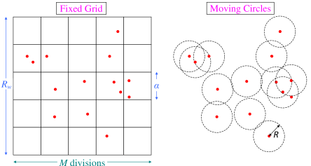
(a)                                                     (b)

Figure 1: The calculation procedure of factorial moments of second order, $F_{2}$, in (a) and correlation integral, $C$, in (b).

The other method to address correlations is by the correlation integral, $C$, [20]. This quantity reveals how a system is structured at different scales $R$, which represent differences between values of any physical quantity that we want to study and it is evaluated to be

$$C(R)=\frac{2}{\left\langle{N_{m}\left(N_{m-1}\right)}\right\rangle_{e}}{\left\langle\sum_{i=1}^{N_{m}}\sum_{j=1}^{i-1}\theta(|\vec{x}_{i}-\vec{x}_{j}|\leq R)\right\rangle_{e}}\;.$$ (3)

Here, for a specific scale $R$ we form freely moving disks with radius $R$ which is measured from the centre of the disk. The disks are line segments, circles or spheres in an embedding space of one, two or three dimensions, respectively. We position the centre of the disk at each point $i$ of our data with coordinates $\vec{x}_{i}$ and count the number of points enclosed by the disk. This is carried out by evaluating the distance $s_{D}$ of all the rest points $j$ with coordinates $\vec{x}_{j}$ from the point $i$, which in a $d$-dimensional embedding space, is $s_{D}\equiv|\vec{x}_{i}-\vec{x}_{j}|=\left[\sum\limits_{k=1}^{d}\left(x_{ik}-x_{jk}\right)^{2}\right]^{1/2}$. The distance $s_{D}$ is compared with the scale $R$. The procedure for two dimensions is shown in Fig. 1(b). The correlation integral for a fractal data set of dimension $d_{F}$ behaves as function of $R$ as

$$C(R)\propto R^{d_{F}}\;,$$ (4)

which has slope in a logarithmic diagram equal to the fractal dimension $d_{F}$.

Thus, the quantities $F_{2}$ and $C$ are interrelated since they determine the fractal dimension of a point set. As we will show in the present work, it is possible to obtain a direct relation between $F_{2}$ and $C$. This relation turns out to be very useful whenever the correlation analysis is performed in an ensemble of point sets each containing a small number of points. Such a situation necessarily occurs in applications in particle physics when the correlations between particles of a specific species are calculated through averaging over a large number of events. Then, it often appears the case that the number of particles of interest per event -and consequently the set of their coordinates which form the considered point set- is very small. As a typical example we refer the reader to the correlation analysis of proton transverse momenta in ion collisions [21]. Then, the calculation of $F_{2}$ becomes prohibitive as the size of cells in the embedding space becomes very small. Here we will show how we can profit from the derived relation between $F_{2}$ and $C$ in order to develop a very efficient computational tool allowing to perform calculations in this prohibited region which is crucial for the detection of critical correlations [22, 23].

The structure of this paper is as follows. In section 2 we establish a relation between $C$ and $F_{2}$ which allows to pass our calculations from one to the other. We, also, stress the advantages by working with the correlation integral. Further issues, related to this correspondence in cases of data of varying multiplicities, are discussed in A. In section 3 we develop a fast computational algorithm for calculating the correlation integral which is, also, passed to $F_{2}$. We probe its effectiveness with respect to conventional methods of calculation. In section 4 we apply the $C-F_{2}$ correspondence and our calculation technique to analyse several data sets, which reside at embedding spaces with one to three dimensions. We, also, note the limitations which a finite data set exhibits. In section 5 we study a situation where a data set contains the needed information with a large percentage of unwanted “noise” and show how our method can reveal this information. We analyse a simulated data set with these attributes and show that conventional techniques would be inadequate. In section 6 we summarise our conclusions. Our paper is accompanied by the source computing code, as supplemental file, which can be used for the relevant calculations.

2 Mapping between $F_{2}$ and C

The factorial moments of the second order, $F_{2}$ (1) and the correlation integral, $C$ (3) show an underlying similarity. Both measure the number of pairs in a set of points at some scale. Indeed, to calculate $F_{2}$, one has to count the number of points $N$ that fall inside the cells of a certain partition $M$. Then, in eq. (1) the number $N(N-1)$ is recorded, which is twice the number of pairs. Also, in the calculation of $C$, one has to count the number $N$ of points that fall within a disk of radius $R$ centred at a specific point. This is the number of pairs that can be formed with this specific point. The procedure is repeated for all the points, so that in the end we have all the pairs that can fit within disks of radius $R$. This similarity allows us to map between $F_{2}$ and $C$.

To find the average total number of pairs, $\left\langle N_{p}(M)\right\rangle_{e}$, used in $F_{2}$, which corresponds to a partition $M$, we have to add for all cells of this partition the average quantity $\left\langle N(N-1)\right\rangle_{e}$ of each cell, which appears in eq. (1). Solving the equation for this quantity and having in mind that the pairs in $F_{2}$ are counted twice, we get

$$\left\langle N_{p}(M)\right\rangle_{e}=\frac{1}{2}\sum\limits_{c}{{{\left\langle{N(N-1)}\right\rangle}_{e}}}=\frac{1}{2}\frac{{\left\langle{{N_{m}}}\right\rangle_{e}^{2}}}{{{M^{d}}}}{F_{2}}(M)\;.$$ (5)

The pairs which correspond to a scale $R$, are recorded in $C$ through the theta function appearing in eq. (3). This function counts one for each point $j$ falling within the disk of radius $R$ centred at point $i$ and zero otherwise. Thus, the average number of pairs, $\left\langle N_{p}(R)\right\rangle_{e}$, counted in $C$ and corresponding to the scale $R$, are taken from eq. (3) to be

$$\left\langle N_{p}(R)\right\rangle_{e}={\left\langle\sum_{i=1}^{N_{m}}\sum_{j=1}^{i-1}\theta(|\vec{x}_{i}-\vec{x}_{j}|\leq R)\right\rangle_{e}}=\frac{{{{\left\langle{{N_{m}}\left({{N_{m}}-1}\right)}\right\rangle}_{e}}}}{2}C(R)\;.$$ (6)

We, now, demand the pairs which correspond to $C$ at the scale $R$ to be equal to the pairs which correspond to $F_{2}$ at the partition $M$. Then, with the help of eqs. (5) and (6), we get

$$\left\langle N_{p}(M)\right\rangle_{e}=\left\langle N_{p}(R)\right\rangle_{e}\Rightarrow$$

$$\Rightarrow\frac{1}{2}\frac{\left\langle N_{m}\right\rangle_{e}^{2}}{M^{d}}F_{2}(M)=\frac{\left\langle N_{m}\left(N_{m}-1\right)\right\rangle_{e}}{2}C(R)\Rightarrow C(R)=\frac{\left\langle N_{m}\right\rangle_{e}^{2}}{\left\langle N_{m}\left(N_{m}-1\right)\right\rangle_{e}}\frac{1}{M^{d}}F_{2}(M)\;.$$ (7)

If the number of multiplicities per event are constant eq. (7) is reduced to

$$C(R)=\frac{N_{m}}{N_{m}-1}\frac{1}{M^{d}}F_{2}(M)\;.$$ (8)

We have to relate the scale $R$ to the partition $M$. Let our working space in the evaluation of $F_{2}$ have measure $V_{w}=R_{w}^{d}$, with $d$ being the embedding space dimension. The measure of each cell in the partition $M$ is $V_{F_{2},d}=a^{d}$. Obviously $a=\frac{R_{w}}{M}$. Then it should hold that

$$R\propto a=\frac{R_{w}}{M}\;.$$ (9)

In the evaluation of $C$, the scale $R$ is a radius which defines distance around a certain point in order to search for other points which are enclosed within the boundaries of the disk. This measure is $V_{C,1}=2R$ in one dimension as line segment, $V_{C,2}=\pi R^{2}$ in two dimensions as circle and $V_{C,3}=\frac{4}{3}\pi R^{3}$ in three dimensions as sphere. Demanding equal measures for $F_{2}$ and $C$ we have that

$$V_{F_{2},d}=V_{C,d}\;.$$ (10)

Substituting $V_{F_{2},d}$ in eq. (10) we find the exact relation of the scale $R$ to the partition $M$, for each space dimension $d$

$$R=\beta_{d}\frac{R_{w}}{M},\;\;\beta_{1}=\frac{1}{2},\;\beta_{2}=\frac{1}{\sqrt{\pi}},\;\beta_{3}=\sqrt[3]{\frac{3}{4\pi}}\;.$$ (11)

Eq. (7) or (8) with eqs. (11) allow for the mapping between correlation integral and the second order factorial moment as

$$C(R)=a_{m}^{-1}\left(\frac{R}{\beta_{d}R_{w}}\right)^{d}F_{2}\left(\frac{\beta_{d}R_{w}}{R}\right)\;,$$ (12)

$$F_{2}(M)=a_{m}M^{d}C\left(\frac{\beta_{d}R_{w}}{M}\right)\;,$$ (13)

where $a_{m}$ is given by

$$a_{m}=\frac{\left\langle N_{m}\left(N_{m}-1\right)\right\rangle_{e}}{\left\langle N_{m}\right\rangle_{e}^{2}}\;,\;\;\;a_{m}=\frac{N_{m}-1}{N_{m}},$$ (14)

for varying or constant multiplicities $N_{m}$ per event, respectively. In the Appendix we elaborate more specifically how to deal with situations where our data contain events with different multiplicities $N_{m}$.

The above relation (11) between scales $R$ and partitions $M$ holds exactly at scales well below the scale which corresponds to the size of the “box” containing all the data so that boundary effects are negligible. To understand why, let us consider in $d=$2 dimensions a cell of size $a$ which can contain data points and all around it exist other cells which, also, can contain data points. The corresponding disk is of radius $R=a/\sqrt{\pi}$ and is movable so that one point is placed at its center to count other points enclosed within. Two points may exist within the cell which have distance $a\sqrt{2}$ and the cell will count them. The corresponding disk cannot count them, since their distance is greater than the radius of the disk. However, if the disk, which is freely moving, is placed with its center at one point within the cell it can find another point in one of the adjacent cells to form a pair within the disk. The outcome is equivalent, since the cell and the disk have equal surfaces, and thus equal probability of finding points enclosed within their domain. The situation is altered, though, at low partitions. Let us suppose that we prepare a set of points existing within a window of side $R_{w}$. According to eq. (11), the corresponding disk has radius $R=R_{w}/\sqrt{\pi}$. A point placed at one corner of the window, which represents our unique cell for $M=1$, can form a pair with every other point within the window. But if we place the disk with its center close to one corner of the window it cannot count as partner of the pair a point with greater distance than its radius. Now, the disk cannot find another point outside the window to form a pair, since the window encloses all the existing data points. As $M$ increases the boundary cells cover a decreasing percentage of the whole surface and so the boundary effects diminish. To deal with this effect, when calculating $F_{2}$ through $C$, we assign to the $M=1$ partition not only the pairs enclosed within disks of radius $R=R_{w}/\sqrt{\pi}$, but, also, all the pairs outside this disk. In this way the $M=1$ result of $F_{2}$ calculated from the grid and from the $C$ will always coincide. For the few low $M$ partitions where the grid and $C$ calculations may differ due to boundary effects, we can shift slightly the boundary between the scales which correspond to adjacent $M$. According to eq. (11), an integer $M^{\prime}$ will correspond to an exact value of scale $R^{\prime}$ and an integer $M^{\prime\prime}=M^{\prime}-1$ will correspond to an exact value of scale $R^{\prime\prime}>R^{\prime}$. Normally, every scale $R$ obeying $R^{\prime\prime}>R>R^{\prime}$ should, also, correspond to $M^{\prime}-1$. Instead, we can extend slightly the interval of scales corresponding to $M^{\prime}$, so that the $F_{2}$ grid calculations coincide, on the average, with the calculations through $C$ at the low $M$ partitions. As $M$ increases this extension will have no effect, as the interval $R^{\prime\prime}-R^{\prime}$ shrinks.

However, apart from the similarity that enables the establishment of a correspondence between $F_{2}$ and $C$, crucial differences between the factorial moments and the correlation integral do exist, which make apparent the advantages we have by working with $C$. These differences are the following:

a) The grid, which is needed to calculate $F_{2}$ at partitions $M$, is fixed and not directly related to the data. The results we get depend on the grid location relative to the data and the size of the analysis space, controlled by $R_{w}$. In contrast, in order to calculate $C$, we form disks which locate themselves according to the data, since each disk has as its center, each time, a data point. Consequently, in $C$ we always get a unique result for the same data set, whilst in $F_{2}$ our result is grid depended.

b) Depending on the location of the grid we form to calculate $F_{2}$ at a specific partition $M$, a group of points may or may not be included within a cell. For this reason we may repeat the calculation for the same $M$ with grids slightly shifted in different directions and then take as result the average. This “grid averaging”, on one hand, severely increases the time needed to complete the calculation. On the other hand, the grid averaging does not ensures us that we have counted the maximum possible number of points per cell. During the averaging one grid may split a group of points which could be fitted within the size of a cell of the specific partition, while another grid may split another group of points. Then, when we take the average, the result will be lower than the possible maximum value. This effect may be important when we are dealing with events with low multiplicities. On the contrary, with the moving disks of $C$ we never lose points at a specific scale $R$. Our result is always the same (at the highest possible value), so we do not need to perform any kind of averaging, saving, also, computation time.

c) The grid of $F_{2}$ entangles scales. For example, let us consider a partition $M$ with cells of size $a$ in two dimensions. Then two points, located close to the diagonal corners of a cell and separated by distance $s_{D}\simeq a\sqrt{2}$, are enclosed within the cell and counted for the estimation of $F_{2}$. However, if two points exist in the data set, which have the same distance but their connecting line is positioned paralleled to one grid axis, then they cannot be enclosed in a cell of size $a$, no matter where we move the grid parallel to its axes. Also, even when $s_{D}<a$ the two points may be separated in different cells. So a pair of points with a specific distance $s_{D}$ may or may not belong to a specific partition $M$. Unlike $F_{2}$, $C$ provides a pure correspondence of the distance of a pair to the scales $R$. There is a clear “cut” for the number of pairs $N(R)$ which belong to a specific scale $R$. A pair with distance $s_{D}=R$ will always be enclosed to measuring disks with radius $R^{\prime}\geq R$ and, so, it can be assigned unambiguously to all scales $>R$.

d) The grid calculation of $F_{2}$ introduces larger errors with the respect to $C$. The source of these errors may be the possible splitting of pairs and the entanglement of scales. Also, the odd or even partitions $M$ may introduce artificial fluctuations. This occurs, for example if there is a large concentration of data points at some space location, e.g. at the center of the grid. Then, if an odd partition encloses most of these points in a cell, then the even partition will systematically split most of them, leading to considerably different results. Counter to $F_{2}$, $C$ calculations, in general, provide smoother distributions, with lower errors. This can be important at situations where the detection of a weak signal is needed.

e) The partitions $M$ which are estimation points for $F_{2}$ is a natural number. Thus, we estimate $F_{2}$ at discrete points. This does not matter, of course, at large $M$, but at low partitions, close to unit, we have discontinuities. In contrast $C$ can be calculated at any scale $R$, so we can have practically a continuous calculation even for the large scales, which correspond to low $M$.

f) There is a difference which has no effect on the actual calculation, but it is related to the physical understanding we may have on the system. The correlation integral $C$ reveals how the system behaves at different scales, which are direct physical quantities. On the contrary, the results of $F_{2}$ are connected to the partitions $M$, which are artificial quantities, giving us an indirect sense of the scales. The physical quantities are the sizes of the cells, with which, qualitative, $M$ are inversely related. To reach at the exact quantitative relation between $M$ and scales, we have to utilize the size of the whole space where we perform our analysis.

Finally, we note that the correlation integral, which is connected to distances between pair of points (doublets), has been related here to the factorial moments of the second order, which, also, count pairs. Therefore, $C$ cannot be related to higher factorial moments, $F_{q}$, $q=3,4,\ldots$, since they describe how the number of higher multiplets (triplets, quadruplets, etc.) change as scale (or partition) varies.

3 A fast computational technique

In a conventional algorithm of calculation of $F_{2}$, one first has to form a specific grid of partition $M$. Then, for every event, the points in every cell have to be counted. In the calculation of $C$, one first has to define a specific scale $R$. Then, for every event, disks of radius $R$ have to be formed centred at each point and the other points which reside within the disk have to be counted. In sort, a conventional algorithm first forms a grid with a certain partition or disks of certain scale and then counts the points that correspond to this partition or scale.

In the previous section we saw that the correlation integral, in contrast to the factorial moments, allows for a clear “cut” in the correspondence of pair of points to specific scales $R$. This attribute allows for an improvement of the algorithm we shall use to calculate $C$. We can assign each pair to a specific scale $R$. In this way we know in advance all the disks where this specific pair belongs to. These are all the disks with radius $\geq R$. In the 2-dimensional case, we know that this pair fits exactly in a “ring” with radius about $R$, as it is depicted in Fig. 2(a). This picture of a 2-dimensional ring can be generalised in one dimension, where we have two line segments, each with length $dR$, located symmetrically at distance $R$ from a point and in three dimensions, where we have a spherical shell of thickness $dR$ and radius $R$. However, we shall call the technique we are developing with the name ring for every dimension $d$.

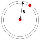
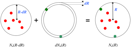
(a)                                       (b)

Figure 2: (a) Two points at distance $R$ form a pair that fits in a ring of radius $\sim$R centred at one of the points. (b) Here each pair of points is represented by one point, the one that is not positioned at the centre of the ring or disk, so, the dots represent pairs. The ring or disks appearing in this figure represent all similar rings or disks of equal size formed to analyse our data set, they are not positioned at a fixed location, but instead they have collected all the points that fall within the domain they define. To count the pairs within the disk $R$ we can count the pairs of disk $R-dR$ and add the pairs within the ring with radii $R-dR$ and $R$.

So, in a data set we can form all possible pairs within the event, for all events, calculate the distance between the two points of the pair and then assign each pair to the relevant ring. In the end of the process we have the number of pairs $dN_{p}(R)$ which correspond to this particular ring. To find the number of pairs which correspond to a set of disks with radius $R$ we have to sum all the rings with radius up to $R$. Equivalently, as it is described in Fig. 2(b), if we know the number of pairs for the set of disks $N_{p}(R-dR)$, we simply have to add the pairs of the ring $dN_{p}(R)$ to find the number of pairs in the set of disks $N_{p}(R)$. The underlying physical meaning here is that the disks of radius $R$ in $C$ are connected to the cumulative probability function, while the rings of thickness $dR$ are connected to the probability density.

In general, we can define as many rings as the number of our estimation points, $N_{D}$, at which we want to calculate $C$. Thus, it becomes obvious the advantage we have through this technique. With only one reading of data we have the value of $C$ at all scales, whilst in the conventional way we had to read all the data for each scale for which we wanted to calculate $C$. As a result in the new technique, the time needed to complete the calculation is little influenced by $N_{D}$. The average number of pairs in a ring due to the events is

$$\left\langle dN_{p}(R)\right\rangle_{e}=\frac{1}{N_{e}}\sum_{e}dN_{p}(R),$$ (15)

where the sum is formed with one reading to all $N_{e}\times\frac{1}{2}N_{m}\cdot(N_{m}-1)$ pairs of the data set. Then the average number of pairs corresponding to scale $R$ is simply

$$\left\langle N_{p}(R)\right\rangle_{e}=\sum_{r\leq R}\left\langle dN_{p}(r)\right\rangle_{e}=\left\langle N_{p}(R-dR)\right\rangle_{e}+\left\langle dN_{p}(R)\right\rangle_{e}\;.$$ (16)

Then, through eq. (6), we can evaluate $C$ as

$$C(R)=\frac{2}{\left\langle N_{m}\left(N_{m}-1\right)\right\rangle_{e}}\left\langle N_{p}(R)\right\rangle_{e}\;.$$ (17)

However, the situation becomes a little more complicated if we want to calculate the errors due to fluctuations imposed by the different events. To accomplish this, we have to evaluate the error in the number of pairs within the disk of radius $R$, due to different events. This error reads

$$\delta\left\langle N_{p}(R)\right\rangle_{e}=\sqrt{\frac{1}{N_{e}-1}\left\langle\left[N_{p}(R)-\left\langle N_{p}(R)\right\rangle_{e}\right]^{2}\right\rangle_{e}}=$$

$$=\sqrt{\frac{1}{N_{e}(N_{e}-1)}\left\{\sum_{e}\left[N_{p}(R)\right]^{2}-\frac{1}{N_{e}}\left[\sum_{e}N_{p}(R)\right]^{2}\right\}}\;.$$ (18)

The sum over the number of pairs in each ring per event, $N_{p}(R)$, for all events can be found by adding the results of all events and so it requires only one reading of all data. But the sum of the squares of the number of pairs in each ring per event, $\left[N_{p}(R)\right]^{2}$, entails to find for every event separately the number $N_{p}(R)$. Consequently, after putting the $\frac{1}{2}N_{m}(N_{m}-1)$ pairs, available in an event, into rings, we have to read all the available $N_{D}$ rings to find out the result. This process performs data reading $N_{D}\times N_{e}\times\frac{1}{2}N_{m}(N_{m}-1)$ times. Despite this increase in processing time, the process remains advantageous, as we shall see later on. The total error in $C$, using eq. (17), can be found to be

$$\delta C(R)=C(R)\sqrt{\left[\frac{\delta\left\langle N_{p}(R)\right\rangle_{e}}{\left\langle N_{p}(R)\right\rangle_{e}}\right]^{2}+\left[\frac{\delta\left\langle N_{m}\left(N_{m}-1\right)\right\rangle_{e}}{\left\langle N_{m}\left(N_{m}-1\right)\right\rangle_{e}}\right]^{2}}\;,$$ (19)

where we have included the case of varying $N_{m}$ per event.

Through mapping between $F_{2}$ and $C$ we can use the above technique to calculate $F_{2}$, as well. Thus, we can calculate $C$ and then, using eq. (7) or (8), we can evaluate $F_{2}$. More directly, we can follow similar steps with the ones in the calculation of $C$ with the ring technique. The application of this technique in this case, again, involves finding the distances between all the pairs in the data set with only one reading of data. Through eqs. (11) we can assign each distance to a partition $M$. At the end of reading of the whole data set we have formed rings with respect to partitions, $\left\langle dN_{p}(M)\right\rangle_{e}$. Then we can find the total number of pairs corresponding to the partition $M$ by adding the relevant rings as in eq. (16):

$$\left\langle N_{p}(M)\right\rangle_{e}=\sum_{l\geq M}\left\langle dN_{p}(l)\right\rangle_{e}=\left\langle N_{p}(M+1)\right\rangle_{e}+\left\langle dN_{p}(M)\right\rangle_{e}\;.$$ (20)

Then, through eq. (5), we have

$$F_{2}(M)=\frac{M^{d}}{\left\langle N_{m}\right\rangle_{e}^{2}}2\left\langle N_{p}(M)\right\rangle_{e}\;.$$ (21)

So, in the evaluation of $F_{2}$ with this technique, called $F_{2,CI}$, we utilize the distances $R$ between pairs, through movable disks, as it is done in $C$ and the relation $M(R)$ between partitions and scales to form rings of partitions, $dN_{p}(M)$. Thus, this procedure determines the central quantity which is the pairs that correspond to a certain partition $N_{p}(M)$. At conventional calculations of 2nd order factorial moments, $F_{2,c}$, we estimate the number of pairs at a certain partition directly by counting points within fixed cells. These calculation schemes of $F_{2}$ can be summarised as

$$R,\;M(R),\;\left\langle dN_{p}(M)\right\rangle_{e}\stackrel{{\scriptstyle F_{2,CI}}}{{\longrightarrow}}\left\langle N_{p}(M)\right\rangle_{e}\stackrel{{\scriptstyle F_{2,c}}}{{\longleftarrow}}\sum\limits_{c}\left\langle{N(N-1)}\right\rangle_{e}\;.$$ (22)

The benefit we have by evaluating $F_{2}$ utilizing rings, is that we can achieve even more reduction in processing time compared to the conventional techniques, at least at the cases, as we shall see later on, where the conventional computing technique of $F_{2}$ is more time consuming than the relevant one of $C$.

As far as the error calculation is concerned, the total error of $F_{2}$, for the ring technique (using eq. (21)) or conventional manner (using eq. (5)), can be found to be

$$\delta F_{2}(M)=F_{2}(M)\sqrt{\left[\frac{\delta\left\langle N_{p}(M)\right\rangle_{e}}{\left\langle N_{p}(M)\right\rangle_{e}}\right]^{2}+\left[2\frac{\delta\left\langle N_{m}\right\rangle_{e}}{\left\langle N_{m}\right\rangle_{e}}\right]^{2}}\;,$$ (23)

where the errors $\delta\left\langle N_{p}(M)\right\rangle_{e}$ are evaluated in a similar way to eq. (18) and we have included the case of varying $N_{m}$ per event. The only difference in the error calculation of $F_{2,CI}$ and $F_{2,c}$ comes from the different way the number of pairs at a certain partition is evaluated according to scheme (22). We note that the errors (18) are the mean value errors and the errors (19) and (23) have been calculated through error propagation method. In error calculation throughout this paper we do not use the bootstrap method. In the later, one forms new data sets using the original set by reusing data points repeatedly. For each new data set the standard error calculation is applied. The error calculation is carried out as many times as the number of the formed data sets. So, if there is benefit in time consumption in the error evaluation for one data set with the ring technique compared to conventional method, then this benefit will be multiplied by a factor equal to the number of data sets that will be processed in the bootstrap method.

Next, we come to the discussion on how we assign pairs to scales or partitions. Firstly, in the $C$ calculation, to assign a pair to a ring of radius exactly $R$ (infinitely thin), we calculate the distance $S_{D}$ in the embedding space of dimension $d$, between the two points 1 and 2 of the pair, using the $d$ coordinates $x$ of each point,

$$R=S_{D}=\sqrt{\sum_{i=1}^{d}{\left(x_{1i}-x_{2i}\right)^{2}}}\;.$$ (24)

For the $C$ calculation we divide the maximum available distance in the data $R_{T}$ in bins and we count them with the number $M_{CI}$, with the zero bin corresponding to maximum distances and the maximum bin corresponding to minimum distances. Since, we usually plot $C$ in logarithmic scales, we choose bins which appear equal in such scales. Therefore, we choose a relation between number of bin and scale like

$$R\cdot\tilde{A}_{b}^{M_{CI}}=R_{T},$$ (25)

where $\tilde{A}_{b}>1$, but close to unit. Increasing the number of bins will require to use values of $\tilde{A}_{b}$ closer to unit. In general, if we want to access results until a minimum scale $R_{\min}$ and divide the length between $R_{\min}$ and $R_{T}$ in $M_{CI,\max}$ bins, which will appear equal in a logarithmic axis, then we have to choose $\tilde{A}_{b}$ as

$$\tilde{A}_{b}=\left(\frac{R_{T}}{R_{\min}}\right)^{1/M_{CI,\max}}\;.$$ (26)

On the other hand, if we choose $\tilde{A}_{b}$ and $M_{CI,\max}$ independently, then the lower scale we will be able to access will be

$$R_{\min}=R_{T}\cdot\tilde{A}_{b}^{-M_{CI,\max}}\;.$$ (27)

In eq. (25) $M_{CI}$ is considered as a real number. To convert it to integer for bin purposes we can use the integer part, after solving for $M_{CI}$,

$$M_{CI}=\left[\ln\left(\frac{R_{T}}{R}\right)\frac{1}{\ln(\tilde{A}_{b})}+m_{c}\right],$$ (28)

where the brackets indicate the integer part and $0\leq m_{c}<1$, a parameter through which we can impose a small shift to the scales that correspond to a specific bin. In our calculations we shall take $m_{c}=0$. The last equation assigns different scales within an interval $dR$ to a particular integer $M_{CI}$ and so, our ring has now become finitely thin. Each pair with distance $s_{D}=R$ corresponds to a bin (ring) labelled by $M_{CI}$ according to eq. (28). We, also, choose a maximum number of divisions $M_{CI,\max}$. Pair distances that lead to $M_{CI}>M_{CI,\max}$ are assigned to $M_{CI,\max}$.

Secondly, in the $F_{2}$ calculation, we can evaluate the scale $R=s_{D}$ of a pair and then we can find the relevant $M$ according to eqs. (11), which in that sense is a real number. To convert it to integer we can use

$$M=\left[\frac{\beta_{d}\cdot R_{w}}{R}+m_{f}\right],$$ (29)

where $0\leq m_{f}<1$, a parameter though which we can impose a small shift to the scales that correspond to a specific bin. The value of this parameter has no effect for large values of $M$, however it does affect the low $M$ calculations. We shall choose it appropriately to match as much as possible the calculation of $F_{2}$ though the ring technique with the conventional estimation for the few estimation points of low $M$.

In the following we probe the effectiveness of the new algorithm with respect to conventional techniques. For this reason we perform calculations for the $F_{2}$ with the conventional method, which we shall call $F_{2,c}$. In this algorithm we have improved the time consumption by placing the data points to the specific grid cells they belong to for a particular partition $M$ and not the opposite (i.e. investigate whether each cell contains any of the data points). Also, in this algorithm we do not apply any grid averaging, so for every partition $M$ the calculation is carried out once. Had we done this averaging, the consumed time would be multiplied by the number of different grid locations we performed the calculation. The calculations with our new algorithm for $F_{2}$ are called $F_{2,CI}$, and in these cases we first perform correlation integral like calculations with the ring technique and then map the results to $F_{2}$. We perform calculations for $C$ with the conventional method, which we call $C_{c}$, where for each scale $R$ we form disks of radius $R$ and search for the number of pairs that are enclosed within. The calculations with our new algorithm for $C$, where we first assign pairs to rings are called $C_{r}$. We measure the time consumption for the calculations with these techniques with respect to the number of calculation points, $N_{D}$ (total different partitions $M$ in $F_{2}$, or total different scales $R$ in $C$), the number of events of the data set, $N_{e}$ and the number of multiplicities $N_{m}$ per event (which corresponds to $\frac{1}{2}N_{m}(N_{m}-1)$ number of pairs per event). The $F_{2,CI}$ and $C_{r}$ calculations are carried out with estimation of errors and without errors. All measurements of time are performed in the same computing machine and for data sets we have used uniform distributions in $d$-dimensional spaces. In every projection of the embedding space, the data points we have used are uniformly distributed in the interval $[-5,5]$. We, also, exclude from all measurements the time needed for the output of the final results.

In Figs. 3-5 we present time calculations for $F_{2}$ (in (a)) and $C$ (in (b)) as function of estimation points $N_{D}$, number of events, $N_{e}$ and multiplicities per event, $N_{m}$, respectively, while keeping the remaining parameters constant. The estimation points $N_{D}$ for $F_{2}$ are points that correspond to all partitions up to a higher partition $M_{max}$, so $N_{D}=M_{max}$. The retained constant parameters for every case are so chosen in order to have enough measurements for all techniques with times $<\sim 300$ sec. In each graph we also depict curves appearing as straight lines in the logarithmic plots, which approximate the recorded data for large values of the parameter under investigation. Our aim is to reveal the exponent of the parameter which influences the calculation time. The relation that connects time with the parameter and the accompanying exponent are depicted on the graphs.

Fig. 3(a) shows that for high values of $N_{D}$, time for $F_{2,c}$, for constant $N_{e}$ and $N_{m}$, grows proportionally to $N_{D}^{d+1}$. On the contrary, $F_{2,CI}$, for constant $N_{e}$ and $N_{m}$, grows proportionally to $N_{D}$ with error estimation and is almost independent of $N_{D}$ without error estimation. This reveals the significant advantage which our new algorithm offers when we want to carry out calculations for high number of estimation points, that is when we want to reach low scales $R$, or high partitions $M$. The advantage becomes more significant as the dimension of the embedding space, $d$, increases. From Fig. 3(b) it is evident that for large values of $N_{D}$, time for both $C_{c}$ and $C_{r}$, for constant $N_{e}$ and $N_{m}$, grows proportionally to $N_{D}$. However, time values are lower in the case of the ring technique with the effect being more prominent as the dimension $d$ increases. Also, comparing the conventional techniques for $F_{2}$ and $C$ (Figs. 3(a) and (b) respectively) we find that $C$ is more advantageous, as far as the estimation points are concerned, since it grows proportionally

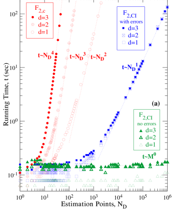
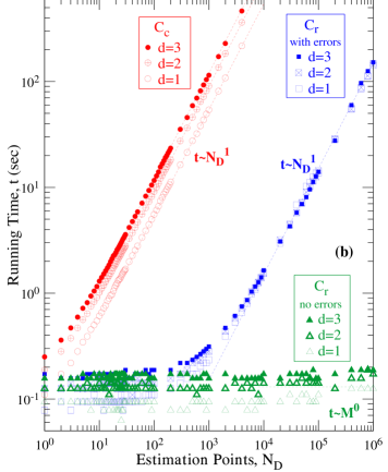
Figure 3: The running time for $F_{2}$ in (a) and $C$ in (b) and for different techniques as function of the estimation points $N_{D}$, for fixed $N_{m}=$10 and $N_{e}=$10000.

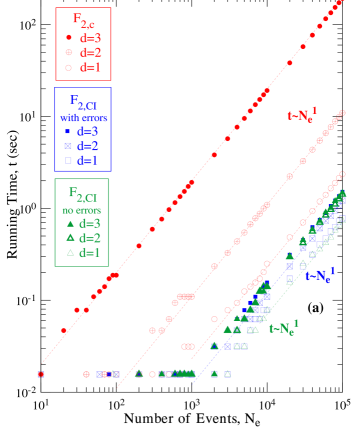
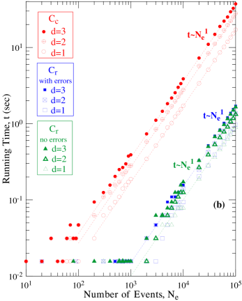
Figure 4: The running time for $F_{2}$ in (a) and $C$ in (b) and for different techniques as function of the number of events $N_{e}$, for fixed estimation points $N_{D}=$30 and $N_{m}=$10.

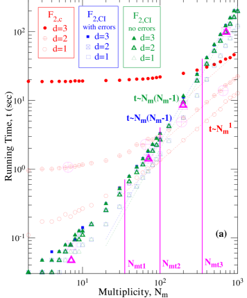
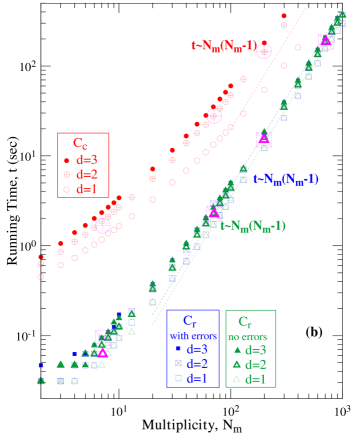
Figure 5: The running time for $F_{2}$ in (a) and $C$ in (b) and for different techniques as function of the multiplicity $N_{m}$, for fixed estimation points $N_{D}=$30 and $N_{e}=$10000. Points with greater size symbols correspond to varying $N_{m}$ cases.

to $N_{D}$ raised to a lower exponent compared to $F_{2}$. The $F_{2}-C$ mapping offers the opportunity to use $C$-based calculations to evaluate $F_{2}$ with the accompanying reduction in time consumption.

In Fig. 4(a)-(b) we see that for high values of number of events $N_{e}$, at constant estimation points $N_{D}$ and multiplicities $N_{m}$, time for all techniques grows proportionally to $N_{e}$.

In Fig. 5(a)-(b) we see how calculation time varies with respect of the multiplicities per event, $N_{m}$, for constant estimation points $N_{D}$ and events $N_{e}$. For high values of $N_{m}$ we expect that time for $F_{2,c}$ grows proportionally to $N_{m}$. However, the conventional method of calculation of the correlation integral, $C_{c}$, as well as, all methods of calculation with the ring technique, $F_{2,CI}$ and $C_{r}$ grow proportionally to the number of pairs $\frac{1}{2}N_{m}(N_{m}-1)$. Thus, it is inevitable that at some value of $N_{m}$ the conventional $F_{2,c}$ will become more effective than the ring technique. The values of $N_{m}$ that this occurs are represented in the graphs by values $N_{mtd}$, where $d$ is the space dimension. $N_{mtd}$ increases with $d$. For the parameters depicted in the graph, $N_{mt1}$ (for $d=1$) is of the order of magnitude of the estimation points, $N_{mt1}\simeq N_{D}$, while as $d$ increases $N_{mtd}$ is pushed at even higher values than the estimation points.

In our calculations we assumed that $N_{m}$ is fixed for all events. Since time consumption is, in all cases, proportional to the number of events, we prove in the Appendix that, when $N_{m}$ varies, the calculation time changes by replacing any function of $N_{m}$ by its average value with respect to the events. Additionally, to test the validity of this finding, we measure the time for processing datasets of events with varying $N_{m}$. Specifically, we prepare files with total $N_{e}=$10000, subdivided to 10 clusters of 1000 events, with each cluster containing events with fixed multiplicity $N_{m,j}=N_{m,i}+jN_{s}$, $j=0,\ldots,9$. We choose appropriately the initial multiplicity $N_{m,i}$ and the step $N_{s}$ in order to have total computational times within the range of Fig. 5. We use again uniform distribution in 2-dimensional embedding space in a rectangle $[-5,5]\times[-5,5]$. We only perform calculations for $d=2$ and for $N_{D}=$ 30 and the resulting points are placed on Fig. 5, using the same symbol with the corresponding fixed $N_{m}$ results, but of greater size. To place a point on the graph, which has as horizontal axis the multiplicity $N_{m}$, we have to evaluate which is the appropriate single value $N_{m}$ in the case of varying $N_{m}$. In the case of $F_{2,c}$ which for constant multiplicity is proportional to $N_{m}$, this is just $\left\langle N_{m}\right\rangle_{e}$. For the rest of cases we calculate the average number of pairs with respect to the number of events, $\left\langle\frac{1}{2}N_{m}(N_{m}-1)\right\rangle_{e}$ $\equiv w$. Then we solve the equation $\frac{1}{2}x(x-1)=w$ and the value $x$ is the one that corresponds to $N_{m}$ which appears to the axes of Fig. 5. We observe that the resulting points fall on the same curve which is formed by the fixed multiplicity cases.

In conclusion, the calculation time for $F_{2}$ and $C$ with the various techniques for large values of the depending parameters grows like the forms listed in Table 1.

Time	Grows like ($\propto$)	Grows like ($\propto$)
	(fixed $N_{m}$)	(varying $N_{m}$)
$t(F_{2,c})$	$N_{D}^{d+1}N_{e}N_{m}$	$N_{D}^{d+1}N_{e}\left\langle N_{m}\right\rangle_{e}$
$t(F_{2,CI}){\rm\;(with\;errors)}$	$N_{D}N_{e}\frac{1}{2}N_{m}(N_{m}-1)$	$N_{D}N_{e}\left\langle\frac{1}{2}N_{m}(N_{m}-1)\right\rangle_{e}$
$t(F_{2,CI}){\rm\;(no\;errors)}$	$N_{e}\frac{1}{2}N_{m}(N_{m}-1)$	$N_{e}\left\langle\frac{1}{2}N_{m}(N_{m}-1)\right\rangle_{e}$
$t(C_{c})$	$N_{D}N_{e}\frac{1}{2}N_{m}(N_{m}-1)$	$N_{D}N_{e}\left\langle\frac{1}{2}N_{m}(N_{m}-1)\right\rangle_{e}$
$t(C_{r}){\rm\;(with\;errors)}$	$N_{D}N_{e}\frac{1}{2}N_{m}(N_{m}-1)$	$N_{D}N_{e}\left\langle\frac{1}{2}N_{m}(N_{m}-1)\right\rangle_{e}$
$t(C_{r}){\rm\;(no\;errors)}$	$N_{e}\frac{1}{2}N_{m}(N_{m}-1)$	$N_{e}\left\langle\frac{1}{2}N_{m}(N_{m}-1)\right\rangle_{e}$

Table 1: The dependence on the involved parameters, $N_{D}$, $N_{e}$ and $N_{m}$ (for large values), of the computation times.

From Table 1 we see that, if we want to decide whether the conventional or the ring method offers faster calculation of $F_{2}$, we have to compare $N_{D}^{d}$ with $\frac{1}{2}(N_{m}-1)$ in the presence of error calculation, or $N_{D}^{d+1}$ with $\frac{1}{2}(N_{m}-1)$ in the absence of error calculation. The exact result, of course, will depend of the accompanying factor of these equations. In the correlation integral case we always have advantage using the ring technique compared to the conventional one. This advantage becomes more significant as the space dimension $d$ increases and is more profound in the absence of error calculation. However, the advantage in time consumption is expected to smear as the multiplicity per event increases. If we want to investigate what goes on at low scales $R$, or high partitions $M$, we must have high number of estimation points. So, it becomes apparent that the maximum number of multiplicities up to which the ring technique retains its effectiveness is pushed to high values, thus, making this technique an indispensable tool in such cases.

The source code of our program in FORTRAN 90 is provided as supplementary material to this paper, containing within explanatory comments for setting the necessary parameters for a specific result.

4 Applications

4.1 Data Analysis

We shall apply the correspondence between $F_{2}$ and $C$ in various data sets. Neglecting boundary phenomena for high scales $R$, $C$ can usually be approximated by the form

$$C(R)\simeq AR^{d_{F}}\;,$$ (30)

in accordance with eq. (4). Then, using eq. (13), we can approximate $F_{2}$ as

$$F_{2}(M^{d})\simeq a_{m}\left(\beta_{d}R_{w}\right)^{d_{F}}A\left(M^{d}\right)^{1-\frac{d_{F}}{d}}\;,$$ (31)

which is in agreement with eq. (2). As it is seen from the last two equations, the exponent of the correlation integral reveals directly the dimension of the data set under investigation, $d_{F}$, whilst $F_{2}$ shows indirectly this dimension through an exponent of the form $1-\frac{d_{F}}{d}$. Both exponents of $C$ and $F_{2}$ can be identified as the slopes in the corresponding logarithmic plots. As an example, in [19] it is shown that the critical opalescence in QCD matter is revealed in transverse momentum space as a power-law behaviour in $q$-order factorial moments $F_{q}\sim(M^{2})^{s_{q}}$, with $s_{q}=(q-1)\left(1-\frac{\tilde{d}_{F}}{2}\right)$ and $\tilde{d}_{F}=\frac{1}{3}$. Thus, while the phenomenon of critical opalescence is expected to appear with a slope in $F_{2}$ equal to $s_{2}=\frac{5}{6}$, the slope of $C$ will be directly equal to the isotherm critical exponent of QCD, $\tilde{d}_{F}=\frac{1}{3}$.

We proceed by dealing with sets with different structures. We shall analyse sets of points which follow the uniform distribution in a region of volume (measure) $V_{d}$ of a space with dimension $d$. These points have constant probability density everywhere in this region, which is

$${}p(x)=\left(V_{d}\right)^{-1}\;.$$ (32)

Here we shall present results for embedding spaces of one and three dimensions. We shall, also, analyse a Lévy set [24] in one dimension. This is produced with steps which follow the probability distribution

$${}p(x)=\nu b^{\nu}\left[1-{\left(\frac{b}{x_{c}}\right)}^{v}\right]^{-1}x^{-1-\nu}\;,$$ (33)

with $\nu=1/3$ and $x$ taking values between $b=10^{-2}$ and $x_{c}=10^{5}$. The $n-$th point in the set of $N_{m}$ multiplicities is the $n$-th successive step, with the first step starting from the origin 0. Before taking each step, apart from the size of the step determined by eq. (33), it is decided whether to move forward or backward using a uniform probability. The increased number of multiplicities, $N_{m}=250$, is needed in order to produce an almost linear part of the $C$-curve in the logarithmic plot. In embedding space of two dimensions, we shall analyse sets of points taken from the Henon [25] and the Ikeda attractor [26]. In embedding space of three dimensions, we shall analyse a Lorentz set which is produced from points taken from the Lorentz attractor [27, 28] with parameters $\rho=28$, $\sigma=10$ and $\beta=8/3$.

In graphs 6-11 we present calculations for the factorial moments $F_{2}$ in (a) and for the correlation integral $C$ in (b). We present examples for all three dimensions $d$ of the embedding space. The calculations for $F_{2}$ are carried out using the correspondence to the correlation integral, $F_{2,CI}$ (open circles). The calculations for $C$, $C_{r}$, as well as those for $F_{2}$ are carried out using the ring technique (open circles). For comparison, we, also, show results for $F_{2}$ through the conventional grid technique, $F_{2,c}$, in (a) and their correspondence to $C$, $C_{F_{2}}$, in (b) (open rectangles). These are limited to fewer estimation points due to the higher need in computation time. In order to match $F_{2,CI}$ with $F_{2,c}$ for the few low values of $M$ we set in eq. (29) $m_{f}=0.27$ in the uniform cases for $d=1$ and $d=3$. In all other cases $m_{f}=0$. In graphs (b) we present a curve, shown as straight line in the logarithmic plots, which has the form of eq. (30) and which approximates $C(R)$ away from the higher scales which are available in the data set. In all cases, but the uniform sets, this curve is produced by a fit in the part of the $C_{r}$-curve which is enclosed within the two slashed lines. In the two uniform cases (Figs. 6(b) and 10(b)) the curve is produced using the exact theoretical value of the set. The curve shown as straight line in the logarithmic plots (a) is eq. (31) for the value $A$ given in graphs (b). The exact form of this equation is depicted on the graphs for each case. From the fit performed on the $C_{r}$-curve (Figs. (b)) we extract the fractal dimension $d_{F,CI}$ with the use of $C$. We, also, perform a fit to the part of $F_{2,CI}$-curve between the two slashed lines in graphs (a), to extract again the fractal dimension, $d_{F,F_{2}}$ from the $F_{2}$ curve. The slashed lines between graphs (a) and (b) are connected trough eqs. (11). Our results are listed in Table 2 for all cases, along with theoretical values, $d_{F,th}$, for the fractal dimension.

Also, it is interesting to observe Fig. 6, where $F_{2}$ is limited within a more constrained interval of values (since it is expected to have zero slop) and the magnitude of statistical fluctuations is shown more clearly. We see that the calculations of $F_{2}$ through the correlation integral experience lower statistical fluctuations compared to the grid technique.

Another interesting observation can be drawn from Fig. 7, where we see that the $F_{2}$ conventional calculations are divided in two separate sets which correspond to odd and even partitions (i.e. $M$ is an odd or even integer, respectively). The Lévy distribution is produced, in this case, with the first step in every event starting from the same point, the origin of the axis. As a result, the one-particle distribution, i.e. the probability of having a particle at a certain interval, exhibits an extremely sharp peek at the origin. The working window is placed so that the origin is at the center of this window. The odd partitions systematically contain a cell enclosing the center of the peek which counts together points existing at both sides of this peek. But the even partitions systematically split the top of the peek to different cells and so they count fewer points. As $M$ progresses to higher partitions, or lower scales, the effect is smoothed out, as the size of the cells becomes smaller that the average width of the distribution and the difference in counting between odd and even partitions diminishes. This situation, of course, can be remedied by applying grid averaging, at the cost of considerable increase of time processing of data, which we do not apply here. On the contrary, the $F_{2}$ calculated using correlation integral like calculations is not affected by the location of the cells at each partition. Since it is using moving disks, it is counting all the pairs corresponding at a certain scale, which is the radius of the disk. In this Lévy case we had full control on where to

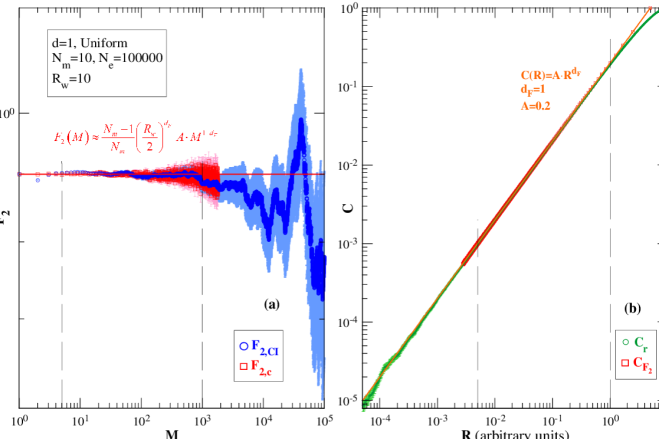
Figure 6: Analysis of a Uniform data set of $N_{e}=100000$ events and multiplicity $N_{m}=10$ in an embedding space of $d=1$ dimension.

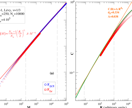
Figure 7: Analysis of a Lévy data set of $N_{e}=10000$ events and multiplicity $N_{m}=250$ in an embedding space of $d=1$ dimension.

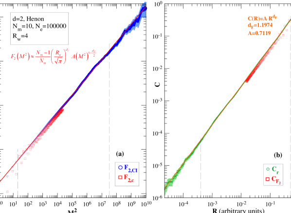
Figure 8: Analysis of a Henon data set of $N_{e}=100000$ events and multiplicity $N_{m}=10$ in an embedding space of $d=2$ dimensions.

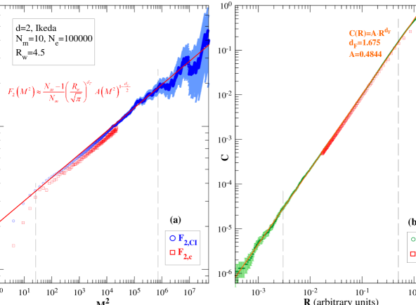
Figure 9: Analysis of an Ikeda data set of $N_{e}=100000$ events and multiplicity $N_{m}=10$ in an embedding space of $d=2$ dimensions.

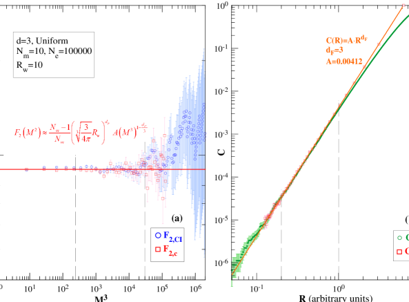
Figure 10: Analysis of a Uniform data set of $N_{e}=100000$ events and multiplicity $N_{m}=10$ in an embedding space of $d=3$ dimensions.

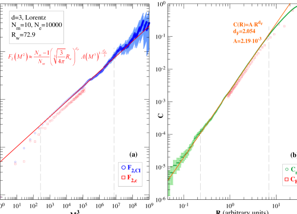
Figure 11: Analysis of a Lorentz data set of $N_{e}=10000$ events and multiplicity $N_{m}=10$ in an embedding space of $d=3$ dimensions.

$d$	data set	$d_{F,CI}$	$d_{F,F_{2}}$	$d_{F,th}$	Ref.
1	Uniform	0.99407$\pm$0.00019	1.00140$\pm$0.00012	1.072$\pm$0.037,1	[29]
1	Lévy	0.3344$\pm$0.0004	0.34342$\pm$0.00006	0.33333
2	Henon	1.1974$\pm$0.0005	1.2174$\pm$0.0005	1.21$\pm$0.01	[20]
				1.220$\pm$0.036,1.258	[29]
				1.21$\pm$0.01,1.25$\pm$0.02	[30]
				1.21,1.22,1.28,1.52,1.36	[31]
2	Ikeda	1.6749$\pm$0.0007	1.6677$\pm$0.0008	1.68,1.72,1.71	[31]
3	Uniform	2.9448$\pm$0.0025	3.001$\pm$0.010	3
3	Lorentz	2.054$\pm$0.002	2.043$\pm$0.005	2.05$\pm$0.01	[20]
				2.049$\pm$0.096,2.062	[29]
				2.05$\pm$0.01	[30]
				2.04,$>$1.90,2.06,2.05,	[31]
				$<$2.14,$<$2.12	[31]

Table 2: Results for the fractal dimension $d_{F}$ calculated by fits on the data depicted on Figs. 6-11 between the slashed lines. $d_{F,CI}$ are extracted by fits on the $C_{r}$ data in graphs (b) and $d_{F,F_{2}}$ are extracted by fits on the data $F_{2,CI}$ in graphs (a). For comparison estimations from corresponding references are provided.

produce the peek. In other cases, like the Henon or the Ikeda attractors, the one-particle distribution exhibit several sharp peeks at different locations. The grid at certain partitions may or may not split these sharp peeks, producing, in the absence of grid averaging, notable differences in adjacent partitions at low $M$.

4.2 Limitations

An infinitely large data set can enable us to access the attributes of the set even at infinitesimal scales. However, we have at hand or can produce a finite number of data points. Inevitably, this leads us to a situation where, as we progress our analysis towards lower scales, the statistical fluctuations will become higher. Then, at even lower scales we will find zero points to fall into our bins. This is the “zero bin” effect. We can make an estimation of the scale where this effect takes place. The constant $A$, in the correlation integral approximation of eq. (30), is related to a scale $R_{max}$, which is connected to the size of the subspace containing the whole data set to be analysed, since at that scale we must have $C(R_{max})=1$. So we can set $A\simeq R_{\max}^{-d_{F}}$ and $C$ can be written as

$${}C(R)\simeq\left(\frac{R}{R_{\max}}\right)^{d_{F}}\;.$$ (34)

Then, let $R_{\min}$ be the scale which corresponds to a bin where we will find, on the average, one pair if we search the whole data set. Beyond that scale we would not expect to find a pair, so the most probable value for $C$ would be zero. Then, using eq. (34) and the definition of $C$, eq. (3), we get

$$C(R)=\frac{2}{{{{\left\langle{{N_{m}}\left({{N_{m}}-1}\right)}\right\rangle}_{e}}}}{\left\langle{{N_{p}}(R)}\right\rangle_{e}}\Rightarrow C(R)=\frac{2}{{{{\left\langle{{N_{m}}\left({{N_{m}}-1}\right)}\right\rangle}_{e}}}}\frac{{\sum\limits_{e}{{N_{p}}(R)}}}{{{N_{e}}}}\Rightarrow$$

$${}\Rightarrow\left(\frac{R_{\min}}{R_{\max}}\right)^{d_{F}}\simeq\frac{2}{{{{\left\langle{{N_{m}}\left({{N_{m}}-1}\right)}\right\rangle}_{e}}}}\frac{1}{{{N_{e}}}}\Rightarrow R_{\min}=R_{\max}\left[\frac{2}{{{N_{e}}\left\langle N_{m}\left(N_{m}-1\right)\right\rangle_{e}}}\right]^{\frac{1}{d_{F}}}\;.$$ (35)

Eq. (35) reveals that the increase of number of events $N_{e}$ and the number of multiplicities $N_{m}$ can help us access lower scales. However, the fractal dimension of the set $d_{F}$ is crucial, since when it acquires higher values, the data set is depleted more rapidly over the scales. Also, we can see this in Figs. 6-11. For example, comparing Figs. 6 and 10, which both describe uniform distributions with the same number of data points, we see that the ratio $\frac{R_{\max}}{R_{\min}}$ acquires a much lower value in the 3-dimensional space compared to the 1-dimensional one, so the statistical fluctuations become prominent at higher scales in three dimensions.

Our aim is to always be able to reach the “zero bin” limit in the data analysis with the techniques presented in this paper, so that there will be no information left uncovered.

4.3 Efficiency Considerations

During the data analysis in experiments it is needed to make corrections in the final results for the detectors efficiency, i.e. for tracks which have not been measured. This amounts to finding out how the results are altered if the number of multiplicities $N_{m}$ per event is increased by a certain ratio $z>1$, so $(z-1)N_{m}$ represents the number of missed tracks per event. We will discuss how the $F_{2}$ and $C$ curves are affected in such a case. We will consider first the case where the number of multiplicities is fixed, i.e. all the events contain the same number of tracks. We will denote by unprimed quantities the initial ones before the increase in their values and by primed quantities the increased ones. The multiplicities $N_{m}^{\prime}=zN_{m}$ correspond to an increase to the total number of pairs per event by a factor $z^{\prime}=z^{2}\frac{N_{m}-1/z}{N_{m}-1}$, since $N_{p}^{\prime}=\frac{1}{2}N_{m}^{\prime}(N_{m}^{\prime}-1)=\frac{1}{2}z^{2}N_{m}(N_{m}-1/z)=z^{2}\frac{(N_{m}-1/z)}{N_{m}-1}\frac{1}{2}N_{m}(N_{m}-1)=z^{\prime}N_{p}$. There are three possibilities:
(a) The number of pairs per event at scale $R$, $N_{p}(R)$, for all scales, is increased by the same ratio and at the same time all the additional multiplicities do not produce a greater distance between them compared to the previous ones. This means that the additional pairs will be distributed among the initial set of scales and proportionally to the initial number of pairs per scale. Thus, all $N_{p}(R)$ are increased by the same ratio $z^{\prime}$. Then from eq. (3) it follows that

$${}C^{\prime}(R)=\frac{2}{N_{m}^{\prime}(N_{m}^{\prime}-1)}\left\langle N_{p}^{\prime}(R)\right\rangle_{e}=\frac{2z^{\prime}}{z^{\prime}N_{m}(N_{m}-1)}\left\langle N_{p}(R)\right\rangle_{e}=C(R)\Rightarrow C^{\prime}(R)=C(R)\;.$$ (36)

Thus, the $C(R)$ curve will remain completely unchanged.
(b) The number of pairs per event at scale $R$, for all scales, is increased by the same ratio but the existence of the additional multiplicities produce some greater distance between them compared to the previous ones. This means that the additional pairs will be distributed among a greater number of scales and proportionally to the initial number of pairs per scale. The $C^{\prime}(R)$ curve will reach the maximum unit value at a greater scale. Now, the number of pairs at scale $R$, $N_{p}^{\prime}(R)$ will be increased by a constant ratio $z^{\prime\prime}<z^{\prime}$ and we will have

$${}C^{\prime}(R)=\frac{2}{N_{m}^{\prime}(N_{m}^{\prime}-1)}\left\langle N_{p}^{\prime}(R)\right\rangle_{e}=\frac{2z^{\prime\prime}}{z^{\prime}N_{m}(N_{m}-1)}\left\langle N_{p}(R)\right\rangle_{e}=\frac{z^{\prime\prime}}{z^{\prime}}C(R)\Rightarrow C^{\prime}(R)<C(R)\;.$$ (37)

The $C(R)$ curve retains the same shape but it is shifted to the right (to greater scales).
(c) The number of pairs per event do not increase proportionally to the initial number of pairs and greater maximum scales may be introduced to the system. In this case the shape of $C$ will change with the increase of additional multiplicities depending on the particular system.

In all the above cases, the $F_{2}$ curve will change according to eq. (13). In (a) the shape of $F_{2}$ will remain the same, but it will increase by a factor $\frac{a^{\prime}_{m}}{a_{m}}=\frac{N_{m}-1/z}{N_{m}-1}$. In (b) the shape of $F_{2}$ will remain the same. Its value will change by a factor $\frac{z^{\prime\prime}}{z^{2}}$. This will lead to an increase, to a decrease or will leave the curve unchanged according to the value of terms $z^{\prime\prime}$ and $z^{2}$. In (c) the shape of $F_{2}$ will in general change, according to the change of the shape of the $C$ curve and eq. (13).

To see the effect of increasing the multiplicity in the case where the number of tracks per event is not fixed, one has to divide the events in subsets of events with fixed multiplicity. Then, the increase of the multiplicity by a certain ratio should be applied at each subset and explore its effect.

We investigate the above considerations by application to specific systems. Our results are shown in Figures 12 and 13, where the $F_{2}$ results are depicted in graphs (a) and the $C$ results in graphs (b). The error depiction is dropped in order to show clearly the important information.

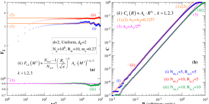
Figure 12: Analysis of Uniform data sets of $N_{e}=10^{6}$ events. Case (i) has points of multiplicity $N_{m,1}=5$ distributed in a rectangle of side $R_{u,1}=5$. In similar manner we have $N_{m,2}=10$ and $R_{u,2}=5$ for case (ii) and $N_{m,3}=10$ and $R_{u,2}=10$ for case (iii).

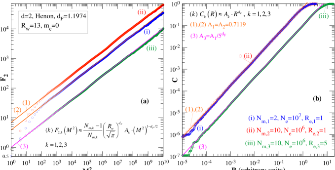
Figure 13: Analysis of Henon data sets. Case (i) involves $N_{e}=10^{7}$ events with multiplicity $N_{m,1}=2$. In similar manner case (ii) corresponds to $N_{e}=10^{6}$ and $N_{m,2}=10$. Case (iii) is similar to case (ii) but the points are expanded in space by a factor $R_{e,3}=5$.

With latin numbers we represent the curves produced from our simulation data and with arabic numbers we represent the theoretical curves that approximate our data curves away from the boundaries (lower scales or greater partitions).

Firstly we deal with a uniform system in a 2-dimensional rectangle and the relevant results are shown in Figure 12. We retain for all $F_{2}$ cases the same analysis window $[-5,5]\times[-5,5]$, with $R_{w}=10$. Initially, we produce a set of points in the rectangle $[-2.5,2.5]\times[-2.5,2.5]$, i.e. with side $R_{u,1}=5$ and multiplicity $N_{m,1}=5$. The corresponding $C$ and $F_{2}$ curves are shown as curves (i) in graph (b) and (a), respectively. Then, we increase the multiplicity per event to $N_{m,2}=10$, still confined to the same rectangle with side $R_{u,2}=5$. The corresponding $C$ curve, (ii) in graph (b) remains unchanged with respect to curve (i) in the same graph, while the $F_{2}$ curve, (ii) in graph (a), is increased by a factor $\frac{a^{\prime}_{m}}{a_{m}}=\frac{4.5}{4}$. In the third case we produce uniformly distributed points in the rectangle $[-5,5]\times[-5,5]$, i.e. with side $R_{u,3}=10$. We, now, observe that the $C$ curve, (iii) in graph (b), while it retains the same slope, which corresponds to $d_{F}=2$, is shifted to greater scales. In this situation we can evaluate exactly the magnitude of the shift. Curve (i) is approximated by the relation $C_{1}(R)\simeq A_{1}R^{2}$. The expansion of the uniform 2-d rectangle by a factor of 2 leads the $C$ curve of case (iii) to acquire the maximum unit value at 2 times the initial value. Thus, Curve (iii) is approximated by the relation $C_{3}(R)\simeq A_{3}R^{2}=\frac{A_{1}}{2^{2}}R^{2}$. The $F_{2}$ curve (iii) compared to curve (i) is increased by a factor $\frac{a^{\prime}_{m}}{a_{m}}=\frac{4.5}{4}$ due to the multiplicity increase and decreased by a factor $\frac{A_{1}}{A_{3}}=\frac{1}{4}$ due to the change of the $C$ curve. The overall effect is a total decrease by a factor of $\frac{4.5}{16}$.

Secondly we take points from the Henon attractor. The relevant results are shown in Figure 13. We retain for all $F_{2}$ cases the same analysis window $[-6.5,6.5]\times[-6.5,6.5]$, with $R_{w}=13$. Initially, we produce $N_{m,1}=2$ points per event using the Henon equations. The result is that all points always fall inside an area in the ($x-y$) plane which can be enclosed by the rectangle $[-1.3,1.3]\times[-1.3,1.3]$. The corresponding $C$ and $F_{2}$ curves are shown as curves (i) in graph (b) and (a), respectively. Then, we increase the multiplicity per event to $N_{m,2}=10$. The resulting points are still enclosed in the same area. The corresponding $C$ curve, (ii) in graph (b) remains unchanged with respect to curve (i) in the same graph, while the $F_{2}$ curve, (ii) in graph (a), is increased by a factor $\frac{a^{\prime}_{m}}{a_{m}}=\frac{1.8}{1}$. In the third case we produce again $N_{m,3}=10$ Henon points per event, but, now, we multiply the $x$ and $y$ coordinates of each point with a factor $R_{e,3}=5$. The result is that the points retain the fractal dimension of the Henon set, but they are enclosed to an area expanded by a factor 5, compared to case (i). Thus, the $C$ curve, (iii) in graph (b), retains the same slope, which corresponds to $d_{F}\simeq 1.2$, but it is shifted to greater scales. To evaluate the magnitude of the shift, we observe that curve (i) is approximated by the relation $C_{1}(R)\simeq A_{1}R^{d_{F}}$, while curve (iii) is approximated by the relation $C_{3}(R)\simeq A_{3}R^{2}=\frac{A_{1}}{5^{d_{F}}}R^{d_{F}}$. The $F_{2}$ curve (iii) compared to curve (i) is overally decreased.

5 A powerful “microscope”

A lot of times in correlation phenomena we want to detect as signal the fractal structure of a data set, exhibited by an exponent $d_{F}$, the fractal dimension of the set. Usually, we have at hand experimental data which do not only contain pure data of the wanted signal, but, also, data behaving as “noise” for our purpose and which may exist at a much higher percentage. Let this noise data be described by a slope of the $C$-curve in logarithmic plot equal to $d_{n}$. If this noise is attributed to uncorrelated random processes defined in $d$ dimensions, then $d_{n}=d$, where $d$ is the dimension of the embedding space. In that case, since the fractal dimension is always lower than the embedding space dimension, $d_{F}<d_{n}$. Then, the correlation integral of our data set can be approximated by a relation of the form

$$C(R)\approx C_{cr}(R)+C_{n}(R)\equiv A\cdot R^{d_{F}}+B\cdot R^{d_{n}}\;,$$ (38)

where $C_{cr}(R)=A\cdot R^{d_{F}}$ is the part which contains our signal, called from now on as critical part and $C_{n}(R)=B\cdot R^{d_{n}}$ is the noise part. The two exponents $d_{F}$ and $d_{n}$ determine the behaviour of $C(R)$ at the scales $R$. As scale $R$ increases, the effect of $d_{n}$ increases and the effect of $d_{F}$ weakens. The opposite is true as scale $R$ decreases. Indeed, we can observe this by defining the ratios

$$e_{cr}(R)=\frac{N_{cr.\;pairs}(R)}{N_{all\;pairs}(R)}=\frac{C_{cr}(R)}{C(R)}=\frac{A\cdot R^{d_{F}}}{A\cdot R^{d_{F}}+B\cdot R^{d_{n}}}$$ (39)

$$e_{n}(R)=\frac{N_{n.\;pairs}(R)}{N_{all\;pairs}(R)}=\frac{C_{n}(R)}{C(R)}=\frac{B\cdot R^{d_{n}}}{A\cdot R^{d_{F}}+B\cdot R^{d_{n}}}\;,$$ (40)

where $e_{cr}(R)$ and $e_{n}(R)$ is the ratio of the critical and noise pairs to the total pairs, respectively, at a specific scale $R$. Differentiating with respect to the scale $R$ we get

$$\frac{d[e_{cr}(R)]}{dR}=\frac{A\cdot B\cdot R^{d_{F}+d_{n}-1}}{\left(A\cdot R^{d_{F}}+B\cdot R^{d_{n}}\right)^{2}}(d_{F}-d_{n})<0$$ (41)

$$\frac{d[e_{n}(R)]}{dR}=\frac{A\cdot B\cdot R^{d_{F}+d_{n}-1}}{\left(A\cdot R^{d_{F}}+B\cdot R^{d_{n}}\right)^{2}}(d_{n}-d_{F})>0$$ (42)

Thus, $e_{cr}(R)$ is a descending function and $e_{n}(R)$ is an ascending function with respect to the scale $R$. Also, $0<e_{cr}(R)<1$, $0<e_{n}(R)<1$, $e_{cr}(R)+e_{n}(R)=1$ and

$$\underset{R\to^{\scriptstyle\;0}_{\scriptstyle\infty}}{\lim}e_{cr}(R)=\underset{R\to^{\scriptstyle\;0}_{\scriptstyle\infty}}{\lim}\left(1+\frac{B}{A}\cdot R^{d_{n}-d_{F}}\right)^{-1}=\;^{\textstyle 1}_{\textstyle 0}$$ (43)

$$\underset{R\to^{\scriptstyle\;0}_{\scriptstyle\infty}}{\lim}e_{n}(R)=\underset{R\to^{\scriptstyle\;0}_{\scriptstyle\infty}}{\lim}\left(1+\frac{A}{B}\cdot R^{d_{F}-d_{n}}\right)^{-1}=\underset{R\to^{\scriptstyle\;0}_{\scriptstyle\infty}}{\lim}\left[1+\frac{A}{B}\cdot\left(\frac{1}{R}\right)^{d_{n}-d_{F}}\right]^{-1}=\;^{\textstyle 0}_{\textstyle 1}$$ (44)

So, at infinite scales our data set behaves as a purely noise set and at infinitesimal scales as a purely critical one. We can use $e_{cr}(R)$ as an estimator of the approach to the fractal behaviour of our data, starting from high scales and moving towards low ones. Moving in the same direction, $e_{n}(R)$ can be used as an estimator of the weakening of the noise behaviour of our data. Indeed, the slope $\kappa(R)$ of $C$ at scale $R$, in a logarithmic graph, can be expressed with respect to these estimators as

$$\kappa(R)=\frac{d\ln(C)}{d\ln(R)}=d_{F}e_{cr}(R)+d_{n}e_{n}(R)=d_{F}e_{cr}(R)+d_{n}\left[1-e_{cr}(R)\right]\;.$$ (45)

Thus, moving in the aforementioned direction, $e_{cr}(R)$ describes how the $C$-slope, an easily observed quantity, changes from $d_{n}$ at high scales to $d_{F}$ at low ones.

We may want to determine the specific scale $R_{q}$ at which $e_{cr}$ acquires a certain value $q$. So

$$e_{cr}(R_{q})=q\Rightarrow\frac{A\cdot R_{q}^{d_{F}}}{A\cdot R_{q}^{d_{F}}+B\cdot R_{q}^{d_{n}}}=q\Rightarrow A(1-q)R_{q}^{d_{F}}=BqR_{q}^{d_{n}}\Rightarrow R_{q}=\left[\frac{A}{B}\frac{(1-q)}{q}\right]^{\frac{1}{d_{n}-d_{F}}}\;.$$ (46)

Of special interest is the value $q=0.5$. At the relevant scale, $R_{t}\equiv R_{0.5}$, the data set transcends from one behaviour to the other. For scales $R<R_{t}$ the critical behaviour becomes the dominant one. This characteristic scale is

$$R_{t}=\left(\frac{A}{B}\right)^{\frac{1}{d_{n}-d_{F}}}\;.$$ (47)

Since $R_{t}$ may not always be reachable from the experimental data set, one may search for a scale, $R_{s}$, where the deviation from the purely “noisy” system starts to show. We can estimate this scale to be located at the point where this deviation exceeds the magnitude of the experimental errors. If the relative experimental error in our measurements is $r$, we can set

$$R_{s}\simeq R_{r}\;.$$ (48)

A common experimental error of the order of 10% would lead to:

$$R_{s}=\left(\frac{9A}{B}\right)^{\frac{1}{d_{n}-d_{F}}}\;.$$ (49)

With the use of eqs. (13) and (38) we can approximate $F_{2}$ as

$$F_{2}(M^{d})\simeq F_{2,cr}(M^{d})+F_{2,n}(M^{d})\equiv a_{m}\left(\beta_{d}R_{w}\right)^{d_{F}}A\left(M^{d}\right)^{1-\frac{d_{F}}{d}}+a_{m}\left(\beta_{d}R_{w}\right)^{d_{n}}B\left(M^{d}\right)^{1-\frac{d_{n}}{d}}\;,$$ (50)

where $F_{2,cr}$ and $F_{2,n}$ is the first and second term of $F_{2}$ which contains the critical and noise contribution, respectively. If $d_{n}\simeq d$, then the noise part of $F_{2}$ will be independent of $M^{d}$.

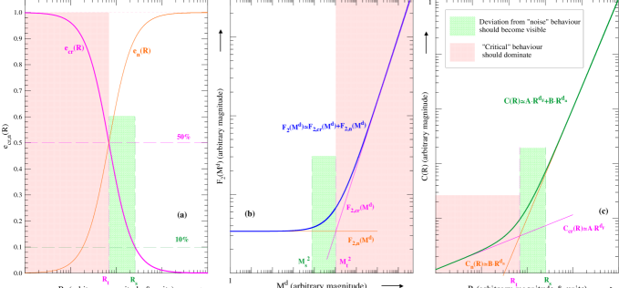
Figure 14: Qualitative description of the behaviour of the estimators $e_{cr}(R)$, $e_{n}(R)$ (a), the factorial moments $F_{2}$ (b) and the correlation integral $C$ (c), in a case where a system with high percentage of noise is analysed.

It may happen that our data set is such that at the higher scanned scales the system exhibits behaviour similar to a purely noise data set. A data set with a high percentage of noise increases the possibility that this will be the case. Then, the only option we have to detect a critical behaviour is to direct our analysis towards the low scales. A qualitative description of what we may encounter is exhibited in Fig. 14. The graphs of $C$ and $F_{2}$ are displayed in (c) and (b), respectively. $C$ at high scales and $F_{2}$ at low partitions cannot be distinguished from the system of pure noise (i.e. the slopes of $C$ and $F_{2}$ are $d_{n}$ and $1-d_{n}/d$, respectively). As we progress our analysis to lower scales (or higher partitions), we arrive at a scale $R_{s}$ (or partition $M_{s}^{d}$) where the deviation from the purely noise system should become apparent. This is shown by the begging of change of slope towards lower values in $C$ and higher values in $F_{2}$. Progressing further, we pass through a scale $R_{t}$ (or partition $M_{t}^{d}$), entering at a territory where the critical set starts to dominate and the slopes of $C$ and $F_{2}$ and tend towards $d_{F}$ and $1-d_{F}/d$, respectively. It is realised that we have to exhaust our analysis down to the lower scales to extract all possible information hidden in the data. Of course, the lower scale analysis will be stopped, either by the approach to the “empty bin” limit (eq. (35)), where the statistical fluctuations will increase immensely, or by the approach to scales corresponding to the detector resolution. In Fig. 14(a) we depict the estimators $e_{cr}(R)$ (eq. (39)) and $e_{n}(R)$ (eq. (40)). The first can be used as an estimator of the approach to the region of scales with the critical behaviour. In such a scenario, as this depicted in Fig. 14, the value of $B$ can be determined by a fit on the $C$-curve at high scales, while the evaluation of $A$ necessitates the appearance of a segment of the $C$-curve clearly departing from the territory with slope $d_{n}$.

We apply the above to a more concrete example. We form by simulation a data set of $N_{e}=10^{6}$ events with multiplicity $N_{m}=26$, consisting mostly of noise events and with some events containing the signal to be detected (critical events) in an embedding space of $d=2$ dimensions. A critical event is formed by $N_{m}$=26 Lévy walks in two 1-dimensional spaces, in the same way as it was done in section 4 (see eq. (33)) and using the parameters $\nu=1/6$, $b=10^{-7}$ and $x_{c}=10^{-1}$. The final coordinates of our points consist of one coordinate from one 1-dimensional space and one from the other. This external product is expected to form a fractal set with dimension $d_{f}=\frac{1}{6}+\frac{1}{6}=\frac{1}{3}$. We produce 150000 such critical events. A noise event is produced by $N_{m}=26$ uniform points in the 2-dimensional rectangle $[-0.9,0.9]\times[-0.9,0.9]$. To form the data set which contains the signal combined with noise, we pick randomly 10 events from the critical ones, while the rest events are uniform ones, so that to have the total number of $10^{6}$. To form the data set which contains only noise, we separately produce $10^{6}$ uniform events. Our results of the analysis of these data sets are depicted in Fig. 15. On the graphs the quantities with an argument in parenthesis ($(R)$ in graph (b) and $(M^{2})$ in (a)) depict curves which are theoretical approximations on the data, according to eqs. (38) and (50). The quantities without arguments depict the actual calculations on the data. These calculations for the correlation integral $C$ were carried out with the ring technique, involved $N_{D}=$3500 estimation points and were completed with error calculation in 129 s. The calculations for the factorial moments $F_{2}$ were carried out with the ring technique and the correspondence to $C$, involved $N_{D}=$100000 estimation points and were completed with error calculation in 2218 s. The corresponding calculations for $C$ and $F_{2}$, without the error calculation, were carried out within 62 and 39 s, respectively.

On graph (b) we mark the scale $R_{s}\simeq 5.7\cdot 10^{-3}$, where we expect to see indications for departure from the noise behaviour and $R_{t}\simeq 1.5\cdot 10^{-3}$, where we enter the domain of the critical behaviour. The partitions for $F_{2}$ are $M_{s}\simeq 179$ and $M_{b}\simeq 670$, respectively. On the upper left of graph (a) we depict $\Delta F_{2}\equiv F_{2}-F_{2,n}$, which is estimated from the $F_{2}$ of the data containing signal and noise with subtraction of $F_{2,n}$, which corresponds to the pure noise data. As expected, $\Delta F_{2}$ rises proportionally to $\left(M^{d}\right)^{1-\frac{d_{F}}{d}}$. We perform estimation of this quantity up to the partitions where we have pure noise data (the exponent $d_{n}$, which is higher than $d_{F}$, causes the empty bin effect to appear at the pure noise data at lower partitions than the data which contain signal and noise). We observe a gradually strengthened signal at higher values of $M^{d}$, recorded at the increasing value of $\Delta F_{2}$. It should be noted that in analysis of real data, in which the statistics may be much less than in the simulation, the increased statistical fluctuations will hinder $\Delta F_{2}$ to appear clearly at low $M$ partitions, due to its low magnitude. The analysis has to proceed to larger $M$, so that the magnitude of $\Delta F_{2}$ will increase beyond the magnitude of statistical errors and so the trend of the curve will appear clearly.

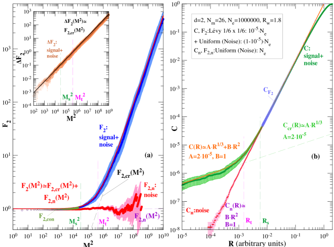
Figure 15: Analysis of a data set from a simulation in an embedding space of $d=2$ dimensions, which contains critical Lévy events of $d_{F}=1/3$ and a high percentage of noise, which is a uniform distribution with $d_{n}=2$. The factorial moments $F_{2}$ are depicted in (a) and the correlation integral $C$ in (b).

On graph (a) we, also, depict the calculations of $F_{2}$ for the signal and noise data set with the conventional way, up to partition $M=150$, (marked as $F_{2,{\rm con}}$) with the corresponding mapping to $C$ in graph (b) (marked as $C_{F_{2}}$). The calculation, performed with no grid averaging which would increase time consumption, took about 15247 s to complete. However, up to this partition we do not observe a clear sign of critical behaviour. We estimate by extrapolation that in order to reach calculations with the conventional routine up to $M_{s}\simeq 179$ it would take $\sim$7 hours, up to $M_{b}\simeq 670$ $\sim$15 days, while to reach $M=100000$, which we easily achieve with our technique, it would require time of the order of magnitude of tens of thousands years.

Thus, we see that, with the ring technique and the $F2-C$ correspondence, we can address large amount of data and scan them up to the very low scales or very high partitions. We have at our hand a very effective “microscope”, which enables us to extract all the information hidden in our data, down to the accuracy set by our measuring equipment. This attribute is due to the negligible time consumption compared to the conventional techniques.

6 Conclusions

We have developed a general mapping between correlation integral and second order scaled factorial moments which constitute two important tools used for the description of correlations in arbitrary data sets. This relation enables us to pass the results of the estimation of one quantity to the other. We are, also, able to form approximations of $C$ and $F_{2}$ that describe the data.

In this way, we can evaluate $F_{2}$ essentially by performing calculations similar to the correlation integral $C$, thus using moving disks, which monitor the data location, instead of a fixed grid. In this way, we can avoid uncertainties due to the grid location and avoid missing pairs corresponding to certain scales or partitions.

Further, we notice that the correlation integral $C$ provides a clear rating of the distance of pairs to scales. Inspired by this, we develop a new computational technique, which counts first the pairs within rings of width $dr$ around $r$ (with $0<r<R$) and then builds the results for disks of radius $R$. The advantage is an extreme reduction of calculation time, which is passed to the calculation of $F_{2}$, as well, through the mapping between $F_{2}-C$. The time reduction becomes more notable as the dimension of the embedding space moves from one to three dimensions. It is, also, negligible in the absence of error calculation, since in that case no further reading of data is required. The technique remains advantageous, as long as the needed number of estimation points remains higher than the average number of pairs per event.

The extreme time reduction enables us to perform scanning of data at minuscule scales $R$ or very high partitions $M$, thus, extracting every piece of information up to experimental accuracy.

We are confident that the techniques developed here can become an indispensable tool in analysing data which contain a very weak signal hidden in a high amount of noise. Also, they can be useful to analyses at embedding spaces of higher dimensions. Especially, we urge for their use in the study of correlation phenomena in heavy-ion experiments whenever modest multiplicities per event are achieved. The analyses with the ring technique can be repeated to all the cases where other techniques have not achieved in reaching the territory of either detector resolution or empty bins.

Acknowledgement. We wish to thank N. Davis for fruitful discussions.

Appendix

Appendix A Distributions for different Multiplicities

Often the analysed data contain events with different multiplicities, $N_{m}$, per event. Let $C_{m}$ and $F_{2,m}$ be the correlation integral and the factorial moments of the 2nd order, respectively, for the subset of our data with constant $N_{m}$. Also, let $C_{t}$ and $F_{2,t}$ be the correlation integral and the factorial moments of the 2nd order, respectively, for the whole set of our data which contain events with different $N_{m}$. We shall see how the above are related.

The fraction of the events with constant $N_{m}$, $N_{e,m}$, to the total number of events, $N_{e}$, is

$$f_{m}=\frac{N_{e,m}}{N_{e}}$$ (A.1)

and apparently

$$\sum\limits_{m}{f_{m}}=1\;.$$ (A.2)

The average number of pairs with respect to the events which we will find at a certain partition $M$ if we analyse all our data is

$$\left\langle N_{p}(M)\right\rangle_{e}=\frac{1}{N_{e}}\sum\limits_{e}N_{p}(M)=\frac{1}{N_{e}}\sum\limits_{m}\sum\limits_{e_{m}}N_{p,m}(M)=$$

$$\frac{1}{N_{e}}\sum\limits_{m}N_{e,m}\left\langle N_{p}(M)\right\rangle_{e,m}=\sum\limits_{m}f_{m}\left\langle N_{p}(M)\right\rangle_{e,m}\;,$$ (A.3)

where with $e_{m}$ we denote the events with certain multiplicity $N_{m}$ and with $\left\langle N_{p}(M)\right\rangle_{e,m}$ the average number of pairs at a certain partition with respect to only these events.

Likewise, the average number of pairs with respect to the events we will find at a certain scale $R$ if we analyse all our data is

$$\left\langle N_{p}(R)\right\rangle_{e}=\sum\limits_{m}f_{m}\left\langle N_{p}(R)\right\rangle_{e,m}\;.$$ (A.4)

The correlation integral for the whole set of our data is

$$C_{t}(R)=\frac{2\left\langle N_{p}(R)\right\rangle_{e}}{\left\langle N_{m}(N_{m}-1)\right\rangle_{e}}=\frac{\sum\limits_{m}f_{m}2\left\langle N_{p}(R)\right\rangle_{e,m}}{\left\langle N_{m}(N_{m}-1)\right\rangle_{e}}=\sum\limits_{m}f_{m}\frac{N_{m}(N_{m}-1)}{\left\langle N_{m}(N_{m}-1)\right\rangle_{e}}\frac{2\left\langle N_{p}(R)\right\rangle_{e,m}}{N_{m}(N_{m}-1)}\Rightarrow$$

$$C_{t}(R)=\sum\limits_{m}g_{m}C_{m}(R)\;\;\;,\;\;\;g_{m}=f_{m}\frac{N_{m}(N_{m}-1)}{\left\langle N_{m}(N_{m}-1)\right\rangle_{e}}\;.$$ (A.5)

The factorial moments of 2nd order for the whole set of our data is

$$F_{2,t}(M)=\frac{2\left\langle N_{p}(M)\right\rangle_{e}}{\left\langle N_{m}\right\rangle^{2}_{e}}=\frac{\sum\limits_{m}f_{m}2\left\langle N_{p}(M)\right\rangle_{e,m}}{\left\langle N_{m}\right\rangle^{2}_{e}}=\sum\limits_{m}f_{m}\frac{N_{m}^{2}}{\left\langle N_{m}\right\rangle^{2}_{e}}\frac{2\left\langle N_{p}(M)\right\rangle_{e,m}}{N_{m}^{2}}\Rightarrow$$

$$F_{2,t}(M)=\sum\limits_{m}h_{m}F_{2,m}(M)\;\;\;,\;\;\;h_{m}=f_{m}\frac{N_{m}^{2}}{\left\langle N_{m}\right\rangle^{2}_{e}}\;.$$ (A.6)

Eqs. (A.5) and (A.6) show the relation between the distributions formed for subsets of our data with constant multiplicity to the whole data distribution. We note that, while

$$\sum\limits_{m}g_{m}=\sum\limits_{m}f_{m}\frac{N_{m}(N_{m}-1)}{\left\langle N_{m}(N_{m}-1)\right\rangle_{e}}=\frac{\left\langle N_{m}(N_{m}-1)\right\rangle_{e}}{\left\langle N_{m}(N_{m}-1)\right\rangle_{e}}=1\;,$$ (A.7)

$$\sum\limits_{m}h_{m}=\sum\limits_{m}f_{m}\frac{N_{m}^{2}}{\left\langle N_{m}\right\rangle^{2}_{e}}=\frac{\left\langle N_{m}^{2}\right\rangle_{e}}{\left\langle N_{m}\right\rangle^{2}_{e}}\geq 1\;.$$ (A.8)

Now the fixed multiplicities distributions $C_{m}$ and $F_{2,m}$ are mapped between each other according to eqs. (12) and (13), thus

$$C_{m}(R)=\frac{N_{m}}{N_{m}-1}M^{-d}F_{2,m}(M)\;.$$ (A.9)

Then for the whole data distributions we have

$$C_{t}(R)=\sum\limits_{m}g_{m}C_{m}(R)=\sum\limits_{m}f_{m}\frac{N_{m}(N_{m}-1)}{\left\langle N_{m}(N_{m}-1)\right\rangle_{e}}\frac{N_{m}}{N_{m}-1}M^{-d}F_{2,m}(M)=$$

$$=\frac{M^{-d}}{\left\langle N_{m}(N_{m}-1)\right\rangle_{e}}\sum\limits_{m}{f_{m}}N_{m}^{2}\frac{2\left\langle N_{p}(M)\right\rangle_{e,m}}{N_{m}^{2}}=\frac{M^{-d}}{\left\langle N_{m}(N_{m}-1)\right\rangle_{e}}2\left\langle N_{p}(M)\right\rangle_{e}=$$

$$\frac{\left\langle N_{m}\right\rangle_{e}^{2}}{\left\langle N_{m}(N_{m}-1)\right\rangle_{e}}{M^{-d}}\frac{2\left\langle N_{p}(M)\right\rangle_{e}}{\left\langle N_{m}\right\rangle_{e}^{2}}\Rightarrow C_{t}(R)=\frac{\left\langle N_{m}\right\rangle_{e}^{2}}{\left\langle N_{m}(N_{m}-1)\right\rangle_{e}}M^{-d}F_{2,t}(M)\;.$$ (A.10)

So, as expected, the mapping of eqs. (12) and (13) can be used either for the constant or for the varying multiplicity distributions.

We, also, consider how time consumption changes when the multiplicity $N_{m}$ per event varies. We can divide our $N_{e}$ in classes which contain $N_{e,m}$ events with fixed $N_{m}$. Each such class takes time $t_{m}$ to be analysed. This time, according to findings of section 3 for fixed multiplicities will be

$$t_{m}=T_{0}N_{e,m}\tilde{f}_{D}(N_{D})\tilde{f}_{N}(N_{m})\;,$$ (A.11)

where $T_{0}$ is a constant, $\tilde{f}_{D}$ is a function of the estimation points and $\tilde{f}_{N}$ is a function of the multiplicity. Then the time $t$ to analyse the whole set will be

$$t=\sum\limits_{m}t_{m}=\sum\limits_{m}T_{0}N_{e,m}\tilde{f}_{D}(N_{D})\tilde{f}_{N}(N_{m})=T_{0}\tilde{f}_{D}(N_{D})\sum\limits_{m}N_{e,m}\tilde{f}_{N}(N_{m})=$$

$$=T_{0}N_{e}\tilde{f}_{D}(N_{D})\sum\limits_{m}\frac{N_{e,m}}{N_{e}}\tilde{f}_{N}(N_{m})=T_{0}N_{e}\tilde{f}_{D}(N_{D})\sum\limits_{m}f_{m}\tilde{f}_{N}(N_{m})=T_{0}N_{e}\tilde{f}_{D}(N_{D})\left\langle\tilde{f}_{N}(N_{m})\right\rangle_{e}$$ (A.12)

So, the time needed to process events with varying multiplicities depends on the average value, with respect to the events, of the function of $N_{m}$ which corresponds to the time consumption for fixed $N_{m}$ cases.

References

- [1] A. Bialas, R. Peshanski, Nucl. Phys. B 273 (1986) 703.
- [2] A. Bialas, R. Peshanski, Nucl. Phys. B 308 (1988) 857.
- [3] J. Wosiek, Acta Phys. Polon. B 19 (1988) 863.
- [4] H. Satz, Nucl. Phys. B 326 (1989) 613.
- [5] N.G. Antoniou, Phys. Lett. B 245 (1990) 624.
- [6] Ph. Brax, R. Peschanski, Phys. Lett. B 346 (1990) 65.
- [7] A. Bialas, R.C. Hwa, Phys. Lett. B 253 (1991) 436.
- [8] M. Ploszajczak, A. Tucholski, P. Bozek, Phys. Lett. B 262 (1991) 383.
- [9] R.C. Hwa, M.T. Nazirov, Phys. Rev. Lett. 69 (1992) 741.
- [10] I.M. Dremin, M.T. Nazirov, Z. Phys. C 59 (1993) 647.
- [11] E.A. De Wolf, I.M. Dremin, W. Kittel, Phys. Rep. 270 (1996) 1.
- [12] X. Cai, C.B. Yang, Z.M. Zhou, Phys. Rev. C 54 (1996) 2775.
- [13] N.G. Antoniou, F.K. Diakonos, C.N. Ktorides, M. Lahanas, Phys. Lett. B 432 (1998) 8.
- [14] N.G. Antoniou, Y.F. Contoyiannis, F.K. Diakonos, A.I. Karanikas, C.N. Ktorides, Nucl. Phys. A 693 (2001) 799.
- [15] N.G. Antoniou, F.K. Diakonos, E. Saridakis, Phys. Rev. C 78 (2008) 024908.
- [16] R.C. Hwa, C.B. Yang, Phys. Rev. C 85 (2012) 044914.
- [17] X.Z. Bai, C.B. Yang, Int. J. Mod. Phys. E 22 (2013) 1350059.
- [18] R.C. Hwa, C.B. Yang, Acta Phys. Pol. B 48 (2016) 23.
- [19] N.G. Antoniou, F.K. Diakonos, A.S. Kapoyannis, K.S. Kousouris, Phys. Rev. Lett. 97 (2006) 032002.
- [20] P. Grassberger, I. Procaccia, Physica D 9 (1983) 189.
- [21] T. Anticic et al., Eur. Phys. J. C 75 (2015) 587.
- [22] N.G. Antoniou, N. Davis, F. K. Diakonos, Phys. Rev. C 93 (2016) 014908.
- [23] N.G. Antoniou, F.K. Diakonos, J. Phys. G: Nucl. Part. Phys. 46 (2019) 035101.
- [24] P.A. Alemany, D.H. Zanette, Phys. Rev. E 49 (1994) R956.
- [25] M. Hénon, Commun. in Math. Phys. 50 (1976) 69.
- [26] K. Ikeda, Optics Commun. 30 (1979) 257.
- [27] E.N. Lorenz, J. Atmos. Sci. 20 (1963) 130.
- [28] D. Viswanath, Physica D 190 (2004) 115.
- [29] J.C. Sprott, G. Rowlands, IJBC, 11 (2001) 1865.
- [30] P. Grassberger, I. Procaccia, Phys. Rev. Lett. 50 (1983) 346.
- [31] J. Jaquette, B. Schweinhart, Commun. Nonlinear Sci. Numer. Simul. 84 (2020) 105163, [arXiv:1907.11182].