Dynamic Adaptive Spatio-temporal Graph Convolution for fMRI Modelling

Abstract

The characterisation of the brain as a functional network in which the connections between brain regions are represented by correlation values across time series has been very popular in the last years. Although this representation has advanced our understanding of brain function, it represents a simplified model of brain connectivity that has a complex dynamic spatio-temporal nature. Oversimplification of the data may hinder the merits of applying advanced non-linear feature extraction algorithms. To this end, we propose a dynamic adaptive spatio-temporal graph convolution (DAST-GCN) model to overcome the shortcomings of pre-defined static correlation-based graph structures. The proposed approach allows end-to-end inference of dynamic connections between brain regions via layer-wise graph structure learning module while mapping brain connectivity to a phenotype in a supervised learning framework. This leverages the computational power of the model, data and targets to represent brain connectivity, and could enable the identification of potential biomarkers for the supervised target in question. We evaluate our pipeline on the UKBiobank dataset for age and gender classification tasks from resting-state functional scans and show that it outperforms currently adapted linear and non-linear methods in neuroimaging. Further, we assess the generalizability of the inferred graph structure by transferring the pre-trained graph to an independent dataset for the same task. Our results demonstrate the task-robustness of the graph against different scanning parameters and demographics.

1 Introduction

A major goal of neuroimaging studies is to develop predictive models to analyze the relationship between whole brain functional connectivity patterns and behavioural traits in order to better characterize brain function and dysfunction. Functional magnetic resonance imaging (fMRI) offers a promising window to investigate the brain activity by measuring the blood oxygenation level which offers a promising proxy to measure the neural activity of the brain. However, extracting the spatiotemporal features from fMRI scans is challenging due to the high dimensionality of the data ($\sim$ 1 M voxels), low signal-to-noise ratio and limited availability of labeled datasets. A standard approach to overcome these challenges is modelling functional connectivity as the pairwise correlations of the time-series of pre-defined brain regions and then feeding these to a classifier either as input features directly[19] or as the underlying structure of a graph[15]. The study of the brain as a graph offers a natural representation of the underlying mechanisms of brain activity[17]. Together with the application of graph theory approaches, the field of network neuroscience has significantly deepened our understanding of brain function and dysfunction. Recently, with the progress of geometric deep learning, graph convolution networks (GCNs) are being exploited in the analysis of fMRI scans[20, 25]. A more befitting model for the dynamics of the brain are spatio-temporal GCNs (ST-GCNs)[24]. [7, 2] recently evaluated the application of ST-GCNs for fMRI analysis for age and gender classification. While these adaptions show a promising direction for modelling the high dimensional signal of the fMRI scan using a spatio-temporal model, the result metrics do not display a significant improvement from shallow non-linear or linear models applied on the flattened correlation matrix. These findings align with the rise of multiple research papers that debate the merits of applying advance deep learning techniques in neuroimaging for phenotype prediction even with scaling of the number of training samples[16, 9]. We hypothesize that these results are attributed to (1) the use of engineered features such as time-series correlations to represent the data of functional parcellations of brain regions, which limits the modelling capability of the deep learning techniques even if a suitable network architecture is implemented. (2) A static graph structure assumes static brain connectivity which contradicts the dynamic nature of brain connectivity [1] and its role in mapping to behavioural traits. (3) The adaption of exact neural network architectures that have shown previous success in other domains however are not well tailored to the nature of fMRI datasets such as the low temporal resolution and the scarcity of labelled samples. To address these issues, we propose a novel spatio-temporal graph convolution architecture with an adaptive graph structure learning. Our approach captures the spatio-temporal dependencies by combining graph convolutions and dilated 1D convolutions. Simultaneously, the graph structure learning module enables the inference of underlying dynamic graph structure. We evaluate our framework on the UKBiobank dataset for the tasks of sex and age classification form resting-state fMRI scans. We compare our results against different baselines as well as ablated versions of the model and we assess the robustness of the trained graph structure for the same task across an independent dataset. The remainder of this paper is ordered as follow: Section 2 describes the key components and the framework of the proposed architecture. Section 3 demonstrates the experiments conducted for the validation of the framework. Section 4 addresses generalizability of the inferred graph structures. Section 5 highlights the limitations of our work. Finally, Section 6 concludes this work and discusses the takeaways and future directions.

2 Methodology

2.1 Preliminaries

We model the brain as $M$ directed dense graphs $\{G^{k}=(V,A^{k})\}_{k=1}^{M}$, $V$ are the nodes of the graph, where each node represent an anatomical region of the brain pre-defined using a template parcellation; $|V|=N$ is the number of regions in the template. $A^{k}$ $\in$ $R^{N\times N}$ represent a directed dense adjacency matrix initialized randomly. The signal on the graph is defined as $X$$\in$$R^{N\times T\times C}$ where $T$ is the number of sampled data-points from the scan and $C$ is the number of channels.

2.2 Temporal lag correction

The low temporal resolution and the existence of the temporal lag patterns in the fMRI signals was highlighted in previous studies[12]. This behaviour can limit the model ability to capture the underlying spatio-temporal signal. To correct for this latency, we compute the first and second derivative of the global time-course signal of each brain region, stack them as 3 channels and apply a $1\times 1$ convolution with a linear activation function before passing the signal to the spatio-temporal blocks.

2.3 Temporal Feature Extraction

We adopt dilated 1D-convolution [13] as our temporal convolution layer (TCN) to capture a node’s temporal trends. Unlike [13] however, we opt for non-causal convolutions, because (i) our objective is learning global temporal representations for a classification task, rather than a generative or horizon prediction task, and (ii) fMRI signals are known to exhibit a temporal lag structure so access to future timepoints could be essential to effectively model intrinsic brain networks. We use gated activation similar to[14]

$$z=\text{tanh}(W_{k,f}*x)\odot\sigma(W_{k,g}*x)$$ (1)

where $*$ denotes a convolution operator,$\odot$ denotes an element-wise multiplication operator, $\sigma$ is a sigmoid function, $k$ is the layer index, $f$ and $g$ denote filter and gate, respectively, and $W_{f}$ and $W_{g}$ are the learnable filter and gate 1D convolutions. We empirically evaluate gated activation against rectified linear unites. We find that gated activation works better for modelling fMRI signal in terms of final metrics and loss convergence.

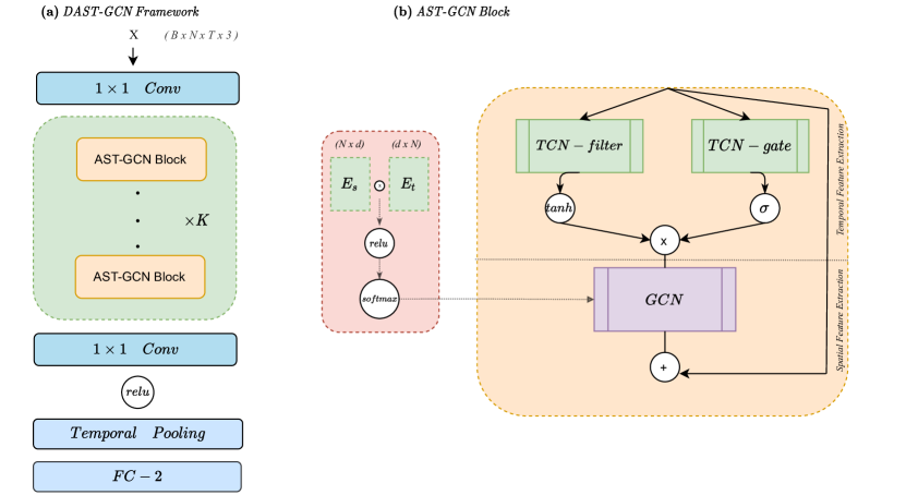
Figure 1: Overview of the DAST-GCN architecture and its main components.

2.4 Spatial Feature Extraction

To extract the spatial correlations of data with unstructured topologies, extending neural networks to process graph-structured data has attracted widespread attention[21]. A series of studies has extended traditional convolution to model arbitrary graphs on spectral [4, 5] or spatial [11, 8] domains. Spectral-based methods use a graph spectral filter to smooth the input signals of nodes. Spatial-based methods extract high-level representations of nodes by gathering feature information of neighbors. [11] shows that graph convolution operation can be well-approximated by 1-st order Chebyshev polynomial expansion and generalized to high-dimensional GCN as:

$$H=A^{{}^{\prime}}XW$$ (2)

where $A^{{}^{\prime}}$ is the normalized adjacency matrix with self-loops. In neuroimaging, the most common approach to pre-define $A$ is a correlation metric between the timecourses. In this work, we inspire from previous studies on adaptive adjacency matrix learning [22, 3] and propose layer-wise graph structure learning module to capture the dynamic spatial dependency across different receptive fields. The normalized adjacency matrix can then be defined as:

$$A^{{}^{\prime}}_{k}=I_{N}+\text{Softmax}(\text{ReLU}(E_{s,k}E_{t,k}))$$ (3)

$E_{s}$$\in$$R^{N\times d}$ and $E_{t}$$\in$$R^{d\times N}$ are trainable source and target dictionaries, where $d$ is a model hyper-parameter. By multiplying $E_{s}$ and $E_{t}$, we derive the spatial dependency weights between the source nodes and the target nodes. We use the $ReLU$ and $Softmax$ activation functions to eliminate weak connections and normalize the adjacency matrix respectively. Finally, the identity matrix $I_{N}$ is added for the self loops.

2.5 Framework of the model

We present the framework of DAST-GCN in Figure 1. First a 1x1 convolution layer with shared weights is applied on each node signal independently to scale up the number of features. Followed by a stack of spatio-temporal blocks. A spatial-temporal block is constructed by a gated temporal convolution layer (Gated TCN) with shared weights across the nodes, an Adaptive graph convolution layer (GCN) and a residual connection. By stacking multiple spatial-temporal layers, DAST-GCN is able to handle spatial dependencies at different temporal levels. Subsequently, Another 1x1 convolution is applied to reduce the node feature dimensions to a single temporal vector, followed by a temporal pooling layer and a dropout layer for regulization. Finally a fully connected layer with softmax activation is applied for the binary classification task.

3 Experiments

3.1 Dataset

We evaluated our pipeline on rs-fMRI scans of 6709 (3255 males / 3454 females, Age = 67.3 $\pm$ 7.2) participants of UKBiobank dataset. First, the provided pre-processed scans were registered to an MNI template followed by applying the AAL atlas [18] to parcellate the brain into N = 116 anatomical regions of interest (ROIs). The time-courses (TR=0.7s, T=490 timepoints) were averaged across the voxels of each ROI to obtain the signal for each node. We conducted binary sex classification and binary age classification for people above and under the age of 70 years to benchmark our framework.

3.2 Experimental Setup

We optimized the model for 200 epochs using Adam optimizer and binary cross-entropy loss with an initial learning rate of 0.001 and cosine scheduler with warm-up. A 5-fold cross-validation scheme was adapted for all the experiments. The models were trained on a Nvidia Tesla P100 GPU with a batch size of 32 and an average training time of 44 s/epoch. After hyper-parameter search, we selected the number of spatio-temporal blocks $K$ = 3, the embedding dimension of the node dictionaries $d$ = 10, the number of filters $f$ = 10 and the kernel size $ks$ = 3 for the temporal convolution layers across the model. The same configuration was selected for both tasks. Parameter sharing and the utilization of 1x1 convolutions across the model enables the development of an efficient model with 11205 trainable parameters. Our implementation is available open-source.

3.3 Experimental Results

We compared the performance of DAST-GCN against the following baseline models:

• SVM-linear: a support vector machine with a linear kernel on the flattened Pearson’s correlation matrix.

• SVM-rbf a support vector machine with a radial basis function kernel on the flattened Pearson’s correlation matrix.

• FCN: a stack of fully connected layers on the flattened Pearson’s correlation matrix.

• BrainNetCNN[10]: a 2D CNN on Pearson correlation matrix.

• 1D-CNN[6]: a 1D CNN on the ROIs timecourses.

• ST-GCN[7]: a static ST-GCN where the nodes features represent ROI timecourses and the edges are defined using thresholded Pearson’s correlation.

For a fair comparison, we conducted a hyper-parameter search for the all the baselines models with the exception of BrainNetCNN[10] and ST-GCN[7] where we used the default parameters recommended by the authors. Moreover, to evaluate the efficiency of our architecture design, we created ablated versions of the model; DAST-GCN_tlc: without temporal lag correction module, DAST-GCN_M=1: only one adjacency matrix is trained throughout the model, DAST-GCN_corr: adjacency matrix is pre-computed as the mean Pearson’s correlation matrix of the training samples, DAST-GCN_undir: a symmetric undirected adjacency matrix, i.e. $E_{t}$ $=$ $E^{T}_{s}$. A comparison of the results of the model against baselines and ablated versions are shown in Table 1.
The results show superior performance of DAST-GCN against baseline models, more predominantly against correlation-based methods which suggest the importance of spatio-temporal modelling of brain activity. This is also supported by the performance of ST-GCN, DAST-GCN_corr and the results from [2] which proves the shortcomings of static pre-defined graph structure based on correlations. The ablation results verify the significance of accounting for the low temporal resolution of the signal before temporal feature extraction. Finally, the comparison of utilizing undirected or single adjacency matrix against $M$ = $K$ dense graphs shows comparable results on sex classifcation and slightly more inferior results on age classification. Further, to assess the practical applicability and relevance of the proposed model in a clinical setting where the number of labeled samples is often scarce, we conducted the classification experiments for the two tasks on different scales of available data points per class (250, 500, 1000, 2500) and report the 5-fold balanced test accuracy results in Fig. 2.

Model	Sex			Age
	Acc.%	Sens.%	Spec. %	Acc.%	Sens. %	Spec. %
SVM-linear	$70.1$$\mathrm{p}\mathrm{m}$1.9	$69.9$$\mathrm{p}\mathrm{m}$2.8	$74.1$$\mathrm{p}\mathrm{m}$3.4	$54.3$$\mathrm{p}\mathrm{m}$1.3	$47.7$$\mathrm{p}\mathrm{m}$1.4	$55.7$$\mathrm{p}\mathrm{m}$1.6
SVM-rbf	$75.1$$\mathrm{p}\mathrm{m}$1.7	$77.4$$\mathrm{p}\mathrm{m}$2.7	$72.5$$\mathrm{p}\mathrm{m}$4	$57.8$$\mathrm{p}\mathrm{m}$1.2	$50.1$$\mathrm{p}\mathrm{m}$1.3	$66.8$$\mathrm{p}\mathrm{m}$7
FCN	$79.2$$\mathrm{p}\mathrm{m}$1.0	$79.5$$\mathrm{p}\mathrm{m}$0.7	$80.4$$\mathrm{p}\mathrm{m}$2.5	$63.1$$\mathrm{p}\mathrm{m}$1.1	$61.3$$\mathrm{p}\mathrm{m}$1.5	$61.1$$\mathrm{p}\mathrm{m}$4.2
1D-CNN[6]	$81.7$$\mathrm{p}\mathrm{m}$1.4	$82.7$$\mathrm{p}\mathrm{m}$2.1	$81.4$$\mathrm{p}\mathrm{m}$0.8	$65.9$$\mathrm{p}\mathrm{m}$0.9	$64.2$$\mathrm{p}\mathrm{m}$1.1	$66.4$$\mathrm{p}\mathrm{m}$2
BrainNetCNN[10]	$77.8$$\mathrm{p}\mathrm{m}$1.8	$78.1$$\mathrm{p}\mathrm{m}$2.3	$77.9$$\mathrm{p}\mathrm{m}$2.9	$60.9$$\mathrm{p}\mathrm{m}$1.2	$60.3$$\mathrm{p}\mathrm{m}$1.8	$62.5$$\mathrm{p}\mathrm{m}$1.3
ST-GCN[7]	$78.4$$\mathrm{p}\mathrm{m}$2.3	$77.2$$\mathrm{p}\mathrm{m}$1.9	$79.8$$\mathrm{p}\mathrm{m}$1.8	$60.5$$\mathrm{p}\mathrm{m}$2.4	$61.4$$\mathrm{p}\mathrm{m}$1.9	$60.1$$\mathrm{p}\mathrm{m}$2.2
DAST-GCN_corr	$78.7$$\mathrm{p}\mathrm{m}$2.1	$77.5$$\mathrm{p}\mathrm{m}$1.8	$79.3$$\mathrm{p}\mathrm{m}$2.5	$61.6$$\mathrm{p}\mathrm{m}$2.9	$61.1$$\mathrm{p}\mathrm{m}$3.4	$62.7$$\mathrm{p}\mathrm{m}$5.6
DAST-GCN_tlc	$82.6$$\mathrm{p}\mathrm{m}$1.3	$82.3$$\mathrm{p}\mathrm{m}$1.2	$82.1$$\mathrm{p}\mathrm{m}$1.3	$61.4$$\mathrm{p}\mathrm{m}$2.6	$60.6$$\mathrm{p}\mathrm{m}$1.7	$61.1$$\mathrm{p}\mathrm{m}$1.3
DAST-GCN_undir	$82.9$$\mathrm{p}\mathrm{m}$1.4	$83.1$$\mathrm{p}\mathrm{m}$1.7	$82.9$$\mathrm{p}\mathrm{m}$1.4	$64.7$$\mathrm{p}\mathrm{m}$4.3	$61.3$$\mathrm{p}\mathrm{m}$2.4	$63.1$$\mathrm{p}\mathrm{m}$2.1
DAST-GCN_M=1	$84.8$$\mathrm{p}\mathrm{m}$0.7	$84.9$$\mathrm{p}\mathrm{m}$0.8	$84.8$$\mathrm{p}\mathrm{m}$0.7	$64.3$$\mathrm{p}\mathrm{m}$3.6	$65.4$$\mathrm{p}\mathrm{m}$2.7	$64.3$$\mathrm{p}\mathrm{m}$3.6
DAST-GCN	$85.3$$\mathrm{p}\mathrm{m}$0.6	$85.4$$\mathrm{p}\mathrm{m}$0.7	$85.3$$\mathrm{p}\mathrm{m}$0.7	$68.6$$\mathrm{p}\mathrm{m}$1.6	$67.9$$\mathrm{p}\mathrm{m}$1.5	$68.4$$\mathrm{p}\mathrm{m}$1.6

Table 1: 5-fold test results (mean $\pm$ standard deviation) of DASTG-GCN against baselines and ablated versions of the model.

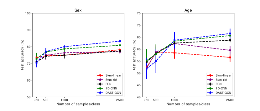
Figure 2: 5-fold scaling performance for DAST-GCN at sex and age classifications against baseline models under different numbers of samples per class. Also shown are the standard-deviation across folds as error-bars.

4 Generalizability

A main challenge of applying deep learning models on neuroimaging datasets is the limited availability of labelled samples and the heterogeneity between fMRI datasets in terms of scanning parameters and participant demographics which restricts the application of pre-trained models across datasets. This explains the wide adoption of linear and shallow non-linear models on engineered features in neuroimaging. However, we hypothesize that a robust graph structure inferred for one task should be the invariant to different scanning parameters and demographics and thus DAST-GCN could be utilized to boost the performance on independent datasets with a limited number of labelled samples. We validated our hypothesis by transferring the graph structure trained on the UKBiobank dataset for sex classification to 120 healthy participants of the REST-meta-MDD dataset [23] (60 males / 60 females, Age = 40.3 $\pm$15.6 years , TR = 1.3 s, T=220 timepoints) for the same task. We chose the DA-STGCN_M=1 version of the model due to the different temporal resolution between datasets and lower number of parameters. We compared the performance of the pre-trained model (DA-STGCN_pretrained) against a model trained from scratch (DAST-GCN_no-pretrain), SVM-linear and SVM-rbf baselines. Test results of the 5-fold cross validation are reported in Table 2. Accuracy of the pretrained model was more than 7 percent point higher than SVM or without pretraining, with less than half the standard deviation. Our results support that the inferred graph structure is robust across datasets with different scanning parameters and demographics, and highlight the potential advantage of applying DAST-GCN in heterogeneous environments where datasets are collected from different sites.

Table 2: 5-fold test results (mean $\pm$ standard deviation) for sex classification on Rest-meta-MDD dataset.

Model	Acc.%	Sens.%	Spec.%
Svm-rbf	61.5$\pm$6.1	65.9$\pm$8.6	56.6$\pm$20.4
Svm-linear	67.6$\pm$10.2	70.7$\pm$13.2	66.3$\pm$12.4
DAST-GCN_nopretrain	66.6$\pm$12.1	69.1$\pm$12.6	62.4$\pm$11.6
DAST-GCN_pretrained	75.0$\pm$4.56	79.6$\pm$8.6	70.0$\pm$10.1

5 Limitations

A good fMRI learning model should not only provide good test metrics but also good explainability in order to advance clinical research. DAST_GCN infers the underlying graph structure while learning, hence offers a direct visualization of potential connectivity bio-markers for the task in hand. However, given training stochasticity and the dynamic and dense representation of the graph, interpetabillity of the visualizations is challenging. A current possible solution for more robust visualizations in our framework would be to restrict the graph to be static and sparse. Though such setup hinders the model performance, its could provide clinical insights specifically when used to study psychiatric disorders. Nevertheless more research on explainability techniques for dynamic graphs is required.

6 Discussion

In this work we proposed a novel spatio-temporal graph convolution model for phenotype prediction from fMRI scans. Our experimental results highlight the advantage of learning a dynamic graph structure versus pre-defined correlation based values. Further, we show that the task-inferred graph structure is robust against the heterogeneity of fMRI datasets and can be effectively transferred across different population demographics and scanning parameters. Finally, our results showcase the quantitative and qualitative advantage of applying deep learning models for phenotype prediction in neuroimaging at different scales and advocate for the development of models that incorporate proper inductive bias and operate on minimally pre-processed derivatives of the raw data.

References

- [1] Allen, E.A., Damaraju, E., Plis, S.M., Erhardt, E.B., Eichele, T., Calhoun, V.D.: Tracking whole-brain connectivity dynamics in the resting state. Cerebral cortex 24(3), 663–676 (2014)
- [2] Azevedo, T., Passamonti, L., Lio, P., Toschi, N.: Towards a predictive spatio-temporal representation of brain data. arXiv preprint arXiv:2003.03290 (2020)
- [3] Bai, L., Yao, L., Li, C., Wang, X., Wang, C.: Adaptive graph convolutional recurrent network for traffic forecasting. arXiv preprint arXiv:2007.02842 (2020)
- [4] Bruna, J., Zaremba, W., Szlam, A., LeCun, Y.: Spectral networks and locally connected networks on graphs. arXiv preprint arXiv:1312.6203 (2013)
- [5] Defferrard, M., Bresson, X., Vandergheynst, P.: Convolutional neural networks on graphs with fast localized spectral filtering. arXiv preprint arXiv:1606.09375 (2016)
- [6] El Gazzar, A., Cerliani, L., van Wingen, G., Thomas, R.M.: Simple 1-d convolutional networks for resting-state fmri based classification in autism. In: 2019 International Joint Conference on Neural Networks (IJCNN). pp. 1–6. IEEE (2019)
- [7] Gadgil, S., Zhao, Q., Pfefferbaum, A., Sullivan, E.V., Adeli, E., Pohl, K.M.: Spatio-temporal graph convolution for resting-state fmri analysis. In: International Conference on Medical Image Computing and Computer-Assisted Intervention. pp. 528–538. Springer (2020)
- [8] Gilmer, J., Schoenholz, S.S., Riley, P.F., Vinyals, O., Dahl, G.E.: Neural message passing for quantum chemistry. In: International Conference on Machine Learning. pp. 1263–1272. PMLR (2017)
- [9] He, T., Kong, R., Holmes, A.J., Nguyen, M., Sabuncu, M.R., Eickhoff, S.B., Bzdok, D., Feng, J., Yeo, B.T.: Deep neural networks and kernel regression achieve comparable accuracies for functional connectivity prediction of behavior and demographics. NeuroImage 206, 116276 (2020)
- [10] Kawahara, J., Brown, C.J., Miller, S.P., Booth, B.G., Chau, V., Grunau, R.E., Zwicker, J.G., Hamarneh, G.: Brainnetcnn: Convolutional neural networks for brain networks; towards predicting neurodevelopment. NeuroImage 146, 1038–1049 (2017)
- [11] Kipf, T.N., Welling, M.: Semi-supervised classification with graph convolutional networks. arXiv preprint arXiv:1609.02907 (2016)
- [12] Mitra, A., Snyder, A.Z., Hacker, C.D., Raichle, M.E.: Lag structure in resting-state fmri. Journal of neurophysiology 111(11), 2374–2391 (2014)
- [13] Oord, A.v.d., Dieleman, S., Zen, H., Simonyan, K., Vinyals, O., Graves, A., Kalchbrenner, N., Senior, A., Kavukcuoglu, K.: Wavenet: A generative model for raw audio. arXiv preprint arXiv:1609.03499 (2016)
- [14] Oord, A.v.d., Kalchbrenner, N., Vinyals, O., Espeholt, L., Graves, A., Kavukcuoglu, K.: Conditional image generation with pixelcnn decoders. arXiv preprint arXiv:1606.05328 (2016)
- [15] Rubinov, M., Sporns, O.: Complex network measures of brain connectivity: uses and interpretations. Neuroimage 52(3), 1059–1069 (2010)
- [16] Schulz, M.A., Yeo, B.T., Vogelstein, J.T., Mourao-Miranada, J., Kather, J.N., Kording, K., Richards, B., Bzdok, D.: Different scaling of linear models and deep learning in ukbiobank brain images versus machine-learning datasets. Nature communications 11(1), 1–15 (2020)
- [17] Sporns, O., Tononi, G., Kötter, R.: The human connectome: a structural description of the human brain. PLoS Comput Biol 1(4), e42 (2005)
- [18] Tzourio-Mazoyer, N., Landeau, B., Papathanassiou, D., Crivello, F., Etard, O., Delcroix, N., Mazoyer, B., Joliot, M.: Automated anatomical labeling of activations in spm using a macroscopic anatomical parcellation of the mni mri single-subject brain. Neuroimage 15(1), 273–289 (2002)
- [19] Vieira, S., Pinaya, W.H., Mechelli, A.: Using deep learning to investigate the neuroimaging correlates of psychiatric and neurological disorders: Methods and applications. Neuroscience & Biobehavioral Reviews 74, 58–75 (2017)
- [20] Wang, L., Li, K., Hu, X.P.: Graph convolutional network for fmri analysis based on connectivity neighborhood. Network Neuroscience pp. 1–13
- [21] Wu, Z., Pan, S., Chen, F., Long, G., Zhang, C., Philip, S.Y.: A comprehensive survey on graph neural networks. IEEE transactions on neural networks and learning systems (2020)
- [22] Wu, Z., Pan, S., Long, G., Jiang, J., Zhang, C.: Graph wavenet for deep spatial-temporal graph modeling. arXiv preprint arXiv:1906.00121 (2019)
- [23] Yan, C.G., Chen, X., Li, L., Castellanos, F.X., Bai, T.J., Bo, Q.J., Cao, J., Chen, G.M., Chen, N.X., Chen, W., et al.: Reduced default mode network functional connectivity in patients with recurrent major depressive disorder. Proceedings of the National Academy of Sciences 116(18), 9078–9083 (2019)
- [24] Yan, S., Xiong, Y., Lin, D.: Spatial temporal graph convolutional networks for skeleton-based action recognition. In: Proceedings of the AAAI conference on artificial intelligence. vol. 32 (2018)
- [25] Zhang, Y., Tetrel, L., Thirion, B., Bellec, P.: Functional annotation of human cognitive states using deep graph convolution. NeuroImage p. 117847 (2021)