Deep Exploration for Recommendation Systems

Abstract.

Modern recommendation systems ought to benefit by probing for and learning from delayed feedback. Research has tended to focus on learning from a user’s response to a single recommendation. Such work, which leverages methods of supervised and bandit learning, forgoes learning from the user’s subsequent behavior. Where past work has aimed to learn from subsequent behavior, there has been a lack of effective methods for probing to elicit informative delayed feedback. Effective exploration through probing for delayed feedback becomes particularly challenging when rewards are sparse. To address this, we develop deep exploration methods for recommendation systems. In particular, we formulate recommendation as a sequential decision problem and demonstrate benefits of deep exploration over single-step exploration. Our experiments are carried out with high-fidelity industrial-grade simulators and establish large improvements over existing algorithms.

1. Introduction

Recommendation systems (RS) play a critical role in helping users find desired content within the ever-expanding universe of information that can be accessed via the Internet. Supervised learning procedures, such as collaborative filtering(Schafer et al., 2007) and content-based filtering(Blanda, 2016) that form the cornerstone of RS, are typically used to model the probability that each piece of content will immediately engage a given user. However, those methods are inadequate when optimizing for delayed user feedback (Joulani et al., 2013; Ktena et al., 2019). In particular, the value of a recommendation can become evident in later interactions with a user, rather than through immediate engagement. For example, a user might submit a positive rating about a news platform after a series of recommendations.

Delays in relevant feedback are prevalent in practical RS. One approach to developing a RS that accounts for delayed feedback is to maintain a model that predicts cumulative future value from interactions with each user, using reinforcement learning (RL) algorithms (Liu and Shih, 2005; Shih and Liu, 2008; Desirena et al., 2019; Iwata et al., 2008; Ie et al., 2019; Theocharous et al., 2015; Chen et al., 2019a; Zheng et al., 2018). Maximizing cumulative future value is especially important when making recommendations that can trigger informative feedback only after subsequent interactions with the user. Although the aforementioned work has demonstrated potential value of RL in RS, sparse and delayed feedback poses challenges to fully realizing the value of RL.

A major challenge to existing RS algorithms arises when positive feedback is rare and tends to arise only after a series of suitable recommendations. For the aforementioned methods to learn from such feedback, enormous quantities of data are required. Indeed, data requirements grow proportionately with the ratio between uninformative and informative feedback (Ganganwar, 2012).

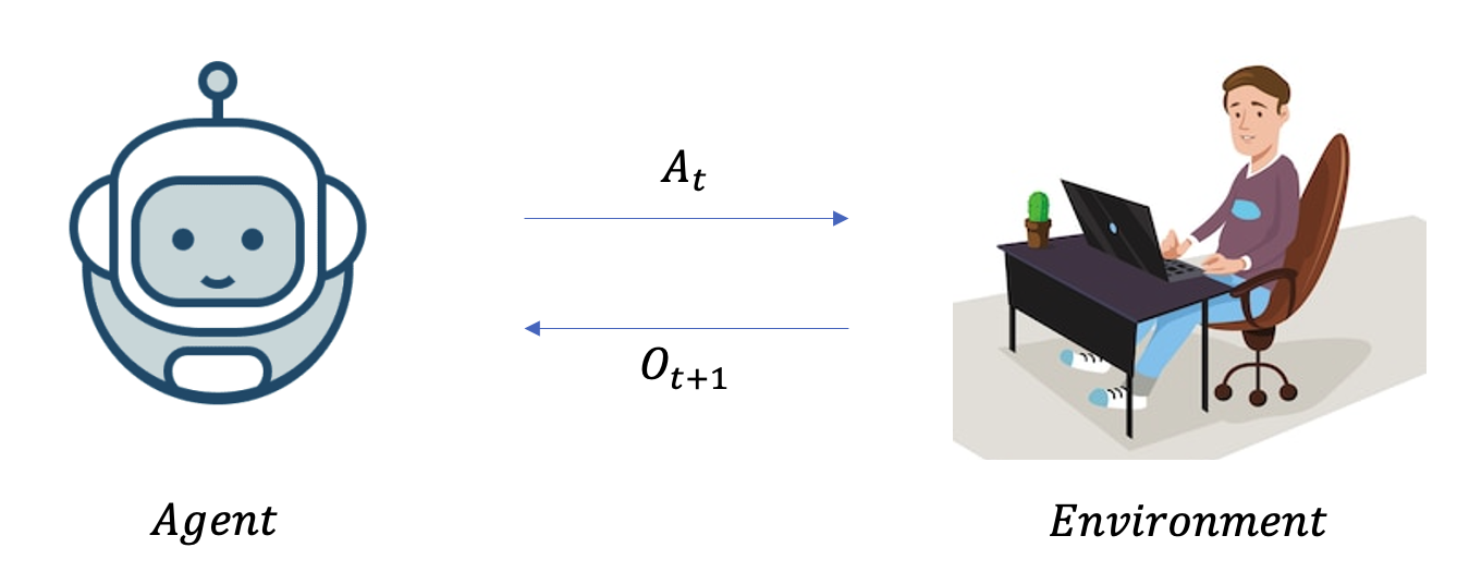
Figure 1. Real-World RS Interface.

Recommendations that aim to elicit informative feedback can dramatically reduce data requirements. Some recent research focuses on bandit-based exploration algorithms such as upper-confidence bound (UCB) (Nguyen-Thanh et al., 2019) and Thompson sampling (Chapelle and Li, 2011) algorithms. However, such exploration strategies are myopic in the sense that they seek information only from immediate user feedback. Deep exploration (Osband et al., 2019) algorithms, on the other hand, further seek information revealed by sequences of rather than individual recommendations. This enables RS to more quickly learn users’ preferences even when their feedback is sparse and delayed.

To the best of our knowledge, this paper is the first to demonstrate the importance of deep exploration in RS. Our work also points to potential benefits beyond user personalization. We develop the first deep exploration algorithm for RS, leveraging randomized value functions (Osband et al., 2019) and epistemic neural networks (ENNs) (Osband et al., 2021). This leads to a proof of concept and empirical evidence that deep exploration can dramatically increase cumulative positive feedback. In Section 2, we review research on RL and bandit learning for RS. In Section 3, we formulate RS design in terms of a sequential decision problem. In Section 4, we present results from case studies that compare common RS designs and bandit exploration designs against one that leverages deep exploration. In doing so, we demonstrate benefits of deep exploration in the face of sparse and delayed feedback. In Section 5, we offer a brief introduction to ENNs. In Section 6, we present a scalable deep exploration algorithm based on randomized value functions and ENNs. In Section 7, we study the effectiveness of deep exploration in RS through a set of experiments, including a toy environment, a high-fidelity e-commerce environment, and a slate ranking environment with parallel user streams. In Section 9, we consider implications of our empirical results, highlighting potential opportunities and possible steps toward productionization.

2. Related Work

In this section, we cover a two topics in RS that are related to sparse and delayed feedback, Contextual Bandit and Exploration as well as Reinforcement Learning.

2.1. Contextual Bandit and Exploration

Contextual bandit algorithms are core to RS research for personalization. Contextual bandit (Langford and Zhang, 2007) is a problem built upon Multi-armed Bandit (Katehakis and Veinott Jr, 1987) where each bandit is contextualized with a representation such that algorithms can make inference across different contexts. In a contextual bandit problem, an agent is asked to select an arm based on the bandit’s context. The agent then uses the collected feedback from the selected arm to update its posterior belief over the bandit. Contextual bandits have been well adopted in the RS community with applications in news article recommendation (Li et al., 2010, 2011), mobile recommendations (Bouneffouf et al., 2012), and even virtual reality (Heyse et al., 2019).

One key advantage of adopting contextual bandit is to leverage the mechanism of exploration. Exploration is a strategic behavior where an agent seeks for information rather than optimizing for reward accumulation. There are multiple strategies to carry out exploration in a contextual bandit environment. The most common exploration strategy in RS is $\epsilon$-greedy (Kamishima and Akaho, 2011; Theocharous et al., 2015; Hu et al., 2017). $\epsilon$-greedy keeps a point estimate for the value of each recommendation and provides a random recommendation with probability $\epsilon$, which may or may not help learn more information about this recommendation. Beyond $\epsilon$-greedy, an agent can adopt the upper confidence bound (UCB) (Garivier and Cappé, 2011; Auer et al., 2002; Guo et al., 2023) strategy, where the agent follows the ”optimism in the face of uncertainty” principle. An agent deems the upper bound of the reward of an arm as its belief of the environment and updates the confidence bound of each arm as it interacts with the environment. The strategy is extended to the LinUCB algorithm (Li et al., 2010) for logistic regression modeling and neural networks (Zhou et al., 2020). Another branch of exploration strategy follows Thompson sampling (Thompson, 1933), where an agent samples from its posterior belief of bandit arms’ rewards and selects the arm with highest sample estimate. Empirical results also show that Thompson sampling outperforms $\epsilon$-Greedy in cumulative positive feedback when only optimizing for immediate user feedback (Chapelle and Li, 2011). The algorithm is also extended to logistic regression (Chapelle and Li, 2011) and neural network versions through ensemble sampling (Lu and Van Roy, 2017; Qin et al., 2022), neural Thompson sampling (Zhang et al., 2020; Osband et al., 2022) or epistemic neural network powered Thompson sampling (Zhu and Van Roy, 2023). However, both UCB-style algorithm and Thompson-sampling-style algorithms for Contextual Bandits remain to explore myopically, i.e. only explore for immediate reward.

2.2. Reinforcement Learning

Recent research in RS has expanded its focus beyond contextual bandits and starts to study the possible design of reinforcement learning algorithms in RS. A key advantage of reinforcement learning over contextual bandit algorithms is that it optimizes beyond immediate reward and maximizes cumulative reward. Using reinforcement learning, we have seen significant user satisfaction improvements with massive dataset available for learning from offline reinforcement learning with value function approximation (Chen et al., 2019b; Rojanavasu et al., 2005; Tang et al., 2019; Golovin and Rahm, 2004; Xu et al., 2023), policy gradient (Chen et al., 2019a) and actor-critic (Chen et al., 2022), but none of the work above focuses on the data efficiency of their solutions and consumes a massive amount of data to produce a reinforcement learning model. Exploration in deep reinforcement learning goes beyond the exploration strategy in bandits. Agents leveraging reinforcement learning aims to optimize long-term cumulative reward and hence needs to seek for information regarding long-term cumulative reward of a policy instead of immediate reward. There has been some recent work (Chen et al., 2021) that starts to focus on the possibility of exploration for users in RS but the design remains to either tweak reward function to incentivize exploration or change the loss function and representation to encode exploration, which only facilitates myopic exploration, where as a deep exploration agent should be able to explore multiple step ahead in a strategic fashion.

In the next two sections, we will define RS in the context of sequential decision making and cover case studies to illustrate the benefit of deep exploration in an intuitive fashion.

3. Problem Formulation

In this section, we formulate RS as a sequential decision problem in which the agent interacts with a community of users. Each user is assigned a distinct positive integer index. At each time $t$, there is a set $\mathcal{U}_{t}$ of active users. Any particular user may be in any combination of these sets across time. At each time, the agent registers an observation from and then provides a recommendation to each active user.

We model interactions as generated by an environment, which is identified by a quintuple $\mathcal{E}=(\mathcal{O},\mathcal{A},r,c,\rho)$:

1. Observation set $\mathcal{O}$: At each time $t$, the agent receives an observation $O_{t,u}$ from each active user $u\in\mathcal{U}_{t}$. The set $\mathcal{O}$ is made up of all possible values of $O_{t,u}$.

2. Action set $\mathcal{A}$: At each time $t$, the agent applies an action $A_{t,u}$ to each active user $u\in\mathcal{U}_{t}$. The set $\mathcal{A}$ is made up of all possible values of $A_{t,u}$.

3. Reward function $r$: The reward function generates a real-valued reward $R_{t,u}=r(O_{t,u})$ based on the observation $O_{t,u}$.

4. Constraint function $c$: It is common in RS that not all items are available to all users at all times. We model this in terms of a constraint function $c$, which prescribes a set of allowed recommendations. In particular, given an observation $O_{t,u}$, the corresponding action is constrained so that $A_{t,u}\in\mathcal{A}_{t,u}=c(O_{t,u})\subseteq\mathcal{A}$.

5. Observation probability function $\rho$: Let $O_{t}=\{(u,O_{t,u})\mid u\in\mathcal{U}_{t}\}$ encode all the agent observes at time $t$, and let $A_{t}=\{(u,A_{t,u})\mid u\in\mathcal{U}_{t}\}$ encode all actions executed by the agent. Let $H_{t}=(O_{0},A_{0},O_{1},\ldots,O_{t})\in\mathcal{H}$ denote the history of the agent’s experience through time $t$. Given $H_{t}$ and $A_{t}$, the observation probability function generates a distribution $\rho(\cdot\mid H_{t},A_{t})=\mathbb{P}(O_{t+1}=\cdot\mid H_{t},A_{t})$.

Agents we will develop address environments of the form we have described. The behavior of an agent can be characterized by a function $\pi_{\rm agent}$, which, for any history $h$, specifies a probability mass function $\pi_{\rm agent}(\cdot\mid h)$ over actions. The agent selects each action according to $A_{t}\sim\pi_{\rm agent}(\cdot\mid H_{t})$. To assess the performance of an agent in a environment $\mathcal{E}=(\mathcal{O},\mathcal{A},r,c,\rho)$ over $T$ timesteps, we compute its cumulative reward

$$\sum_{t=0}^{T-1}\sum_{u\in\mathcal{U}_{t+1}}R_{t+1,u}.$$

Note that this formulation is very general; interactions arising in just about any recommendation system can be modeled in these terms.

In our computational experiments, we posit particular environments and simulate interactions. Realized rewards depend on simulated randomness and thus the initial random seed. To reduce dependence on this seed, we average results over many independent simulations, aiming to compute a close approximation to the expectation over this uncertainty:

$$\mathbb{E}_{\pi_{\rm agent}}\left[\sum_{t=0}^{T-1}\sum_{u\in\mathcal{U}_{t+1}}R_{t+1,u}\right].$$

The subscript $\pi_{\rm agent}$ indicates how actions are selected.

We offer a simple, toy example that serves to crystallize our environment formalism.

Example 1.

Toy Environment
Consider an environment with a single user. In particular, $\mathcal{U}_{t}=\{1\}$ for all $t$. Suppose that, at each time, the agent has a single item at hand – say, a news article – and can choose to recommend it to the user if the user is engaged. No item is available at more than one point in time. The observation set is $\mathcal{O}=\{0,1\}$, with $O_{t,1}=1$ indicating that the user is engaged. The action set is $\mathcal{A}=\{0,1\}$, where $A_{t,1}=1$ indicates recommending the item at hand. The constraint function is defined by $c(1)=\mathcal{A}$ and $c(0)=\{0\}$ to express that the item can only be recommended when the user is engaged. The reward function is defined by $r(o)=o$, indicating a preference for engagement. The observation probability function determines the chances that the user will be engaged in the next timestep.

To offer a concrete, albeit contrived, example, suppose the user remains engaged until receiving ten recommendations over consecutive timesteps, at which points the user is triggered to disengage for one hundred timesteps. We let $Y_{t}$ indicate whether the user is in this disengaged state due to being triggered within the past hundred timesteps. The observation probability function is then defined by

$$\rho((1,1)\mid H_{t},A_{t})=\left\{\begin{array}[]{ll}0&\text{if }Y_{t}=1\\ 1&\text{if }Y_{t}=0.\end{array}\right.$$

In this environment, to maximize cumulative reward over a long horizon, the agent ought to avoid recommending every tenth item but recommend each item between those omissions.

In the next section, we will offer another example environment that embodies sparse and delayed reward and a couple of analyses to explain the benefits of deep exploration.

4. Why Deep Exploration?

Exploration is vital to sample efficiency when faced with sparse and delayed user feedback. Past research on RS has addressed exploration through either $\epsilon$-greedy schemes (Kamishima and Akaho, 2011; Theocharous et al., 2015; Hu et al., 2017) in a reinforcement learning context, or upper confidence bound (UCB) (Nguyen-Thanh et al., 2019; Nakamura, 2015) and Thompson sampling (Chapelle and Li, 2011; Brodén et al., 2018) in a bandit learning context. The first approach randomly perturbs the exploitation strategy without strategically seeking useful information. The latter two approaches are guided by epistemic uncertainty of immediate feedback and lead to myopic exploration. However, actions of an intelligent agent ought to also depend on epistemic uncertainty about delayed feedback. We consider an approach that addresses this via estimating epistemic uncertainty about the optimal value function. Here, the optimal value function of a history-action pair $(h,a)$, denoted by $Q:\mathcal{H}\times\mathcal{A}\rightarrow\mathbb{R}$, refers to the expected reward an agent can accumulate by taking action $a$ at the history $h$ and adhering to an optimal policy thereafter.

Deep exploration refers to a strategic approach that positions an agent to more effectively gather information over subsequent time steps (Osband et al., 2019). In this section, we investigate a deep exploration agent that maintains an approximation to the posterior distribution of the optimal value functions, samples a value function from this distribution upon engaging with a user and adheres to that sample until the user disengages. We refer to the period of user engagement as the user life-cycle. To evaluate the effectiveness of such an agent, we introduce SeqRec, which provides an example environment featuring sparse and delayed rewards. SeqRec represents a RS scenario in which users do not provide any feedback to the agent until the agent’s sequence of recommendations successfully meets their needs.

Example 2.

SeqRec Environment
The SeqRec environment features a fixed set of users across all time steps, such that $\mathcal{U}_{t}=\mathcal{U}=\{1,2,\dots,N\}$ for all $t$. More specifically, the SeqRec environment is defined by the following components, instantiating the environment quintuple $(\mathcal{O},\mathcal{A},r,c,\rho)$:

1. The observation set $\mathcal{O}=\{0,1\}^{2}$. $O_{t,u}=(\text{Satisfied}_{t,u},\text{Leave}_{t,u})\in\mathcal{O}$, where $\text{Satisfied}_{t,u}\in\{0,1\}$ indicates whether user $u$ is satisfied with the recommendation, and $\text{Leave}_{t,u}\in\{0,1\}$ indicates whether the user $u$ intends to disengage with the RS agent. $O_{0}=\{((u,(0,0))\mid u\in\mathcal{U}_{0}\}$.

2. The action set $\mathcal{A}=\{a_{1},a_{2},\text{no-op}\}$, where $a_{1}$ and $a_{2}$ are the only two genres of content for recommendation in the environment.

3. Reward $R_{t,u}=r(O_{t,u})=\text{Satisfied}_{t,u}$.

4. The available set of actions $\mathcal{A}_{t,u}$ at time step $t$ for user $u$ and the constraint function $c$ are defined as

   $$\mathcal{A}_{t,u}=c(O_{t,u})=\begin{cases}\{a_{1},a_{2}\},&\text{if }\text{Leave}_{t,u}=0,\\ \{\text{no-op}\},&\text{if }\text{Leave}_{t,u}=1.\end{cases}$$

5. The observation probability mass function $\rho$ is described by the following deterministic mechanism.

   1. The environment tracks user satisfaction level $Y_{t,u}\in\mathbb{R}$ for every user $u\in\mathcal{U}_{t}$. The environment uses an internal function, $g:\mathcal{U}\times\mathcal{A}\rightarrow\mathbb{R}$, to calculate the change in user satisfaction given an action.

      $$Y_{t+1,u}=\begin{cases}Y_{t,u}+g(u,A_{t,u}),&\text{if }\text{Leave}_{t,u}=0,\\ 0,&\text{if }\text{Leave}_{t,u}=1,\end{cases}$$

   2. The environment tracks each user $u$’s life-cycle length at time $t$ as $L_{t,u}$.

      $$L_{t+1,u}=\begin{cases}L_{t,u}+1,&\text{if }\text{Leave}_{t,u}=0,\\ 0,&\text{if }\text{Leave}_{t,u}=1,\end{cases}$$

   3. Each user $u$ has a target satisfaction level $b_{u}$, where
      $\text{Satisfied}_{t+1,u}=1$ if $Y_{t+1,u}>b_{u}$.

   4. A user decides to disengage with the agent, $\text{Leave}_{t+1,u}=1$, when the user is satisfied with the agent, $Y_{t+1,u}\geq b_{u}$, the user’s satisfaction level drops below 0, $Y_{t+1,u}<0$, or the user’s current life-cycle with the agent is longer than their engagement time budget $L_{t+1,u}>=\tau_{u},\tau_{u}\in\mathbb{N}$.

   5. Lastly we have the probability mass function $\rho$ as

      $$\rho\big{(}O_{t+1}=\{(u,(\text{Satisfied}_{t+1,u},\text{Leave}_{t+1,u}))\mid u\in\mathcal{U}_{t+1}\}\mid H_{t},A_{t}\big{)}=1.$$

SeqRec represents an abstract and simplified model of user interaction. Delayed user feedback in this model is driven by the latent random variable $Y_{t,u}$ that tracks a users level of satisfaction. The agent receives positive feedback when the user’s satisfaction crosses a threshold. Delayed feedback is commonly observed in practical RSs arising in ratings on software applications, cumulative revenue, and total engagement time.

In the following analyses, we will compare deep exploration against $\epsilon$-greedy, Thompson sampling with Gaussian priors, and UCB in a set of case studies using SeqRec.

4.1. SeqRec Sample Complexity: Single-User Case

Consider a SeqRec environment with a single user, $\mathcal{U}=\{1\}$, with a satisfaction change function $g(1,a_{1})=0$ and $g(1,a_{2})=1$. The user’s satisfaction target level and engagement time budget are $b_{1}=\tau_{1}=T$. The agent’s goal is to maximize cumulative reward in SeqRec. The agent has prior knowledge that only one of $a_{1}$ and $a_{2}$ increases the user’s satisfaction level.

The optimal approach here is to consistently apply either action $a_{1}$ or $a_{2}$ until the user disengages, in order to determine which action leads to an increased satisfaction level. If the optimal strategy is not employed, the agent will not receive any positive rewards before the user disengages. In the following analysis, we demonstrate the difference between $\epsilon$-greedy, myopic Thompson sampling, myopic UCB and deep exploration.

Since the agent cannot observe any differences until it applies action $a_{2}$ for $T$ times, there is a unique sequence of recommendations that will reveal the optimal action. Employing the $\epsilon$-greedy strategy, the expected number of user life-cycles required to learn the optimal policy is $\Theta(2^{T})$, as there are $2^{T}$ possible permutations of recommendation sequences in $T$ steps.

Consider a myopic Thompson sampling bandit learning agent with zero-mean Gaussian priors. Given a history $h$, the agent samples from the posterior distributions over the immediate reward and selects the action with the higher reward sample. Since both actions’ immediate reward posteriors are zero-mean Gaussians before receiving any positive feedback, there is a $1/2$ probability of choosing either action $a_{1}$ or $a_{2}$. This probability remains constant after each posterior update until the desired sequence, applying action $a_{2}$ for $T$ times, is discovered. Thus, the expected number of user life-cycles with Thompson sampling is also $\Theta(2^{T})$.

For the myopic UCB strategy, a common approach uses $\sqrt{\frac{\log(t)}{N_{t}(a)}}$ as the exploration bonus, in addition to the marginal reward estimate for a history-action pair, where $N_{t}(a)$ denotes the number of times action $a$ is executed up to timestep $t$. When the user starts to engage, the agent is equally optimistic about $a_{1}$ and $a_{2}$, with identical reward estimates. After each step, the agent reduces its exploration bonus for the selected action, ensuring that the same action will not be chosen in the next timestep. Consequently, the agent continuously alternates between the two actions and never achieves the desired sequence using UCB.

With our approach to deep exploration, the agent maintains an approximate posterior distribution of the optimal value functions $Q$. Initially, the agent’s prior belief assigns a $1/2$ probability to either $Q(h,a_{1})=1$ or $Q(h,a_{2})=1$ for any $h$ that consistently applies $a_{1}$ or $a_{2}$, respectively, and assigns a value of 0 to all other history-action pairs. During any user life-cycle prior to receiving positive feedback, there is a $1/2$ probability that the agent will consistently apply action $a_{2}$ for $T$ times, thereby eliminating the possibility of $Q(h,a_{1})=1$. In expectation, the agent needs $2$ lifecycles to determine $Q(h,a_{2})=1$ when persistently applying $a_{2}$. Consequently, the agent requires only $\Theta(1)$ user life-cycle to learn the optimal policy using the deep exploration strategy.

4.2. SeqRec Sample Complexity: Multi-User Case

Building on Example 1, we now consider a SeqRec environment with $N$ users, denoted as $\mathcal{U}=\{1,2,\dots,N\}$. For some users in $\mathcal{U}$, action $a_{1}$ increases satisfaction by 1, while for others, action $a_{2}$ does the same. For each user $u\in\mathcal{U}$, the action that improves satisfaction is deterministic, and we refer to this action as user $u$’s preferred action. We have $b_{u}=\tau_{u}=T$ for all $u\in\mathcal{U}$, and $N\ll 2^{T}$. The agent aims to optimize cumulative rewards across all users, with prior knowledge that either action $a_{1}$ or $a_{2}$ enhances each user’s satisfaction level. We assume the existence of a function approximator capable of accurately modeling each user’s preferred action after observing the preferred actions of $N/2$ users.

In this example, we extend Example 1 from a single-user environment to a multi-user setting, where learnings from one user can be generalized to serve other users as well. Our aim is to demonstrate that deep exploration remains crucial to an agent’s success in a RS environment with a large user base, even when equipped with powerful generalization capabilities. Since the myopic UCB strategy is unable to identify the optimal policy even in single-user SeqRec, we exclude it from this analysis.

First, we consider the $\epsilon$-greedy and myopic Thompson sampling strategies. As an agent equipped with such strategies have a $\Theta(1/2^{T})$ probability of learning the preferred action for any user $u$ in a life-cycle, the expected number of preferred actions learned after all $N$ users’ first life-cycles is $\Theta(N/2^{T})$. In expectation, $\Theta(2^{T-1})$ life-cycles from all $N$ users are needed for the agent to learn all preferred actions. If the agent undergoes $M$ life-cycles and $M\leq 2^{T-1}$, the expected cumulative reward across the $N$ users in $\mathcal{U}$ is $\Theta(MN/2^{T})$. If $M>2^{T-1}$, the expected cumulative reward is $\Theta(N(M-2^{T-1}))$.

Now, let’s consider deep exploration. This algorithm has a $1/2$ probability of learning each user’s preferred action after a single life-cycle of interaction. In expectation, after the first life-cycles of users in $\mathcal{U}$, the system can perfectly model all users’ preferred actions, yielding an expected cumulative reward of $\Theta(NM)$ in $M$ life-cycles.

The analysis above highlights that intelligent exploration is not only crucial for learning single-user preferences but also for inferring population preferences. Exploration strategies, such as $\epsilon$-greedy, myopic Thompson sampling, and myopic UCB, are ill-suited for problems characterized by sparse and delayed consequences, even when paired with function approximators possessing strong generalization capabilities like deep neural networks. In contrast, deep exploration is much more adept at handling these types of problems.

In the following two sections, we will introduce neural network architectures that are useful for exploration and epistemic uncertainty estimation in RS.

5. Epistemic Uncertainty Estimation via Epistemic Neural Networks (ENN)

Deep neural networks have come a long way in enhancing marginal predictions. Over the past decade, significant advancements have been made in various architectures for RS, such as Neural Collaborative Filtering (He et al., 2018), Wide & Deep (Cheng et al., 2016), and Multi-Head Self-Attention (Wu et al., 2019). These models provide a robust baseline for sophisticated representations of users, recommendations, and their interactions. However, these neural networks are unable to identify what they do not know, i.e., assessing the epistemic uncertainty concerning the environment or the user’s preferences. In this section, we will focus on two neural network strategies for estimating epistemic uncertainty that are compatible with the concept of deep exploration.

5.1. Deep Ensemble (Lu and Van Roy, 2017; Osband et al., 2018, 2016)

Deep ensemble is a neural network architecture that employs an ensemble of neural networks to estimate the posterior distribution of a target variable. This architecture is initialized with $M$ base neural networks, denoted as $\left\{f_{\beta_{1}},\dots,f_{\beta_{M}}\right\}$, with each network parameterized by $\beta_{1},\ldots,\beta_{M}$, respectively. Additionally, $M$ prior neural networks are included, represented as $\left\{f_{\beta_{1}^{p}},\dots,f_{\beta^{p}_{M}}\right\}$.

The prior neural networks are initialized using Glorot sampling and remain unaltered throughout the model’s lifespan (Osband et al., 2018; Glorot and Bengio, 2010). These prior neural networks serve to regularize the posterior parameters, preventing the posterior distribution from collapsing too easily (Zhang et al., 2017; Bartlett et al., 2017).

For a given input $x\in\mathbb{R}^{d_{x}}$, a deep ensemble generates a posterior sample estimate by sampling $z\sim\text{Unif}(\{1,\ldots,M\})$ and computing $\hat{y}=f_{\beta_{z}}(x)+\alpha f_{\beta^{p}_{z}}(x)$. Here, $f:\mathbb{R}^{d_{x}}\rightarrow\mathbb{R}$, and $\alpha\in(0,1)$ is a scaling factor. This method is known as ensemble sampling (Lu and Van Roy, 2017), which approximates Thompson sampling (Qin et al., 2022).

In the context of supervised learning, given a loss function $\mathcal{L}$ and a target variable $y$, an ensemble optimizes each particle $\beta_{z}$ in the ensemble through

(1) $$\beta_{z}=\operatorname*{arg\,min}_{\beta}\mathcal{L}(y,f_{\beta}(x)+\alpha f_{\beta^{p}_{z}}(x)).$$

For simplicity in notation, we denote $h_{\theta,\theta^{p}}(x,z)=f_{\beta_{z}}(x)+\alpha f_{\beta^{p}_{z}}(x)$ as the $z$th neural network in the ensemble, where $h:\mathbb{R}^{d_{x}}\times\{1,\dots,M\}\rightarrow\mathbb{R}$ and $\theta=(\beta_{1},\dots,\beta_{M}),\theta^{p}=(\beta^{p}_{1},\dots,\beta^{p}_{M})$.

5.2. EpiNet (Osband et al., 2021)

Although deep ensemble provides a valuable tool for epistemic uncertainty estimation, its scalability with large deep neural networks remains a challenge. There are two primary bottlenecks of deep ensembles. First, the number of parameters required is $M$ times larger than that of a single neural network. Second, a deep ensemble can only offer $M$ particles sampled from the approximate posterior distribution. EpiNet (Osband et al., 2021) proposes a potential solution to both of these bottlenecks.

EpiNet is an add-on architecture designed for general neural network architectures, enabling epistemic uncertainty estimation and improved joint predictions. Given a neural network function approximator $f_{\beta}:\mathbb{R}^{d_{x}}\rightarrow\mathbb{R}$, parameterized by $\beta$, EpiNet first extracts the last layer representation $\sigma_{\beta}(x)$, where $\sigma_{\beta}:\mathbb{R}^{d_{x}}\rightarrow\mathbb{R}^{d_{\sigma}}$. Next, EpiNet concatenates the representation with an epistemic index $z\in\mathbb{R}^{d_{z}}$ and executes a forward pass on the concatenated vector. The epistemic index can be a one-hot vector or sampled from a Gaussian prior. Similar to deep ensemble, EpiNet also maintains a main network $g_{\eta}$ and a prior network $g_{\eta^{p}}$, where $g:\mathbb{R}^{d_{\sigma}}\times\mathbb{R}^{d_{z}}\rightarrow\mathbb{R}^{d_{z}}$. Hence given a neural network $f_{\beta}$, an input feature vector $x$ and an epistemic index $z$, its target variable estimate $\hat{y}$ with the EpiNet add-on is

(2) $$\hat{y}=f_{\beta}(x)+\left(g_{\eta}(sg[\sigma_{\beta}(x)],z)+\alpha g_{\eta^{p}}(sg[\sigma_{\beta}(x)],z)\right)^{T}z.$$

where $sg[\cdot]$ indicates stop-gradient in backpropagation. In a logistic regression case, $\hat{y}$ goes through an additional Sigmoid function. For simplicity of notation and consistency with the notations for deep ensemble, we denote Equation 2 by $h_{\theta,\theta^{p}}(x,z)$, where $\theta=(\beta,\eta),\theta^{p}=\eta^{p}$. During optimization, given a target variable $y$

(3) $$\theta=\operatorname*{arg\,min}_{\theta}\sum_{z\in\mathcal{Z}}\mathcal{L}\left(y,h_{\theta,\theta^{p}}(x,z)\right).$$

Parameters within $sg[\cdot]$ does not receive gradient flow. Here $\mathcal{Z}$ is a set of epistemic indices sampled from $z$’s prior to approximate the loss across the prior distribution of $z$.

6. A Deep Exploration Agent

In this section, we present an efficient implementation of deep exploration utilizing the Randomized Value Function (RVF) approach (Osband et al., 2019) through ENNs and Deep Q-learning. RVF exhibits two main features. First, it introduces perturbations to the received rewards, encouraging exploratory behavior. Another advantage of RVF is that, given a value function sampled from an ENN, an agent employing the RVF strategy consistently adheres to the policy induced by the value function for the entire user lifecycle, facilitating deep exploration.

6.1. Representations

In this work, we assume that the agent has access to representations of each user, each recommendation, and the historical interactions between users and the RS. We denote the feature representation of a user $u$ as $\psi_{u}\in\mathbb{R}^{d_{u}}$ and that of an action $a$ as $\phi_{a}\in\mathbb{R}^{d_{a}}$. Both $\psi_{u}$ and $\phi_{a}$ are deterministic and remain constant over time. These representations can generally include, for example, demographic information about a user or a text embedding of a recommendation. Additionally, the agent is offered an interaction feature extractor $\textbf{extract\_interact\_features}:\mathcal{H}\times\mathcal{U}\rightarrow\mathbb{R}^{d_{\xi}}$ by the environment. We denote $\xi_{t,u}=\textbf{extract\_interact\_features}(h_{t},u)$ to represent the historical interaction between user $u$ and the agent up to timestep $t$.

6.2. Deep Q-learning

Deep Q-learning has achieved remarkable successes in games (Mnih et al., 2015; Silver et al., 2017) and control tasks (Schrittwieser et al., 2020), where it demonstrates super-human performance. In the context of RS, a deep Q-learning agent uses a neural network to estimate its value function, $Q_{\beta}:\mathbb{R}^{d_{u}}\times\mathbb{R}^{d_{a}}\times\mathbb{R}^{d_{\xi}}\rightarrow\mathbb{R}$, parameterized by $\beta$. Following the problem definition in Section 3, at time step $t$, a deep Q-learning agent selects an action:

(4) $$A_{t}=\left\{\left(u,\operatorname*{arg\,max}_{a\in\mathcal{A}_{t,u}}Q_{\beta}(\psi_{u},\phi_{a},\xi_{t,u})\right):u\in\mathcal{U}_{t}\right\},$$

where $\mathcal{A}_{t,u}=c(O_{t,u})$. The agent explores by either modifying $Q_{\beta}$ or adopting a random exploration approach. For instance, when using $\epsilon$-Greedy as the exploration strategy, with probability $\epsilon$, the agent chooses a random action and follows the value function greedily otherwise. After executing action $A_{t}$, the agent receives a new observation $O_{t+1}$ from the environment and computes reward $R_{t+1}$. If $u\in\mathcal{U}_{t}\cap\mathcal{U}_{t+1}$, the agent stores a transition $(\psi_{u},\phi_{A_{t,u}},\xi_{t,u},R_{t+1,u}$, $\xi_{t+1,u},\mathcal{A}_{t+1,u})$, where $\mathcal{A}_{t+1,u}=c(O_{t+1,u})$, in its replay buffer $\mathcal{D}$ for future learning. It is worth noting that this approach can be easily extended to accommodate multi-step transitions by referencing the last observation generated by user $u$.

After several steps of interaction with the environment, the agent samples data from its replay buffer to improve its value function model $Q_{\beta}$. To stabilize temporal difference learning with deep neural networks, a deep Q-learning agent employs a target neural network strategy, creating a copy of the value function model as the target model $Q_{\beta^{\prime}}$ and copying the parameters from $Q_{\beta}$ to $Q_{\beta^{\prime}}$ every $K$ steps. More formally, with learning rate $\alpha$, the update for $\beta$ is:

(5) $$\begin{split}\beta\leftarrow&\beta-\alpha\nabla_{\beta}\sum_{u\in\mathcal{U}_{t}\cap\mathcal{U}_{t+1}}\Big{[}\Big{(}R_{t+1,u}+\\ &\max_{a\in\mathcal{A}_{t+1,u}}Q_{\beta^{\prime}}(\psi_{u},\phi_{a},\xi_{t+1,u})-Q_{\beta}(\psi_{u},\phi_{A_{t,u}},\xi_{t,u})\Big{)}^{2}\Big{]}\mid_{\beta=\beta_{n}}.\\ \end{split}$$

It is important to note that we did not introduce the discount factor, which is common in RL literature, as we are optimizing for a fixed-horizon cumulative reward.

6.3. Deep Exploration via Randomized Value Function and Epistemic Neural Network

An agent can conduct deep exploration by employing Deep Q-learning through RVF and an ENN, $h^{Q}_{\theta,\theta^{p}}$, in order to estimate the posterior distribution of value functions. $h^{Q}_{\theta,\theta^{p}}$ takes a user representation, an action representation, an interaction feature vector and an epistemic index as input and outputs a value function sample from an approximate posterior distribution. At the beginning of a user life-cycle, a deep exploration agent samples an epistemic index $z_{u}\in\mathbb{R}^{d_{z}}$ from the prior distribution $P_{z}$, and maintains this index throughout the life-cycle. At time step $t$, the deep exploration agent then proceeds to follow a greedy approach:

(6) $$A_{t}=\left\{\left(u,\operatorname*{arg\,max}_{a\in\mathcal{A}_{t,u}}h^{Q}_{\theta,\theta^{p}}(\psi_{u},\phi_{a},\xi_{t,u},z_{u})\right):u\in\mathcal{U}_{t}\right\}.$$

See Section 5 for two potential architectures for $h^{Q}_{\theta,\theta^{p}}$. After taking action $A_{t}$, the agent makes a new observation $O_{t+1}$ from the environment and computes reward $R_{t+1}$.

Similar to a deep Q-learning agent, a deep exploration agent also maintains replay buffers. To incentivize exploration, we adopt the reward perturbation approach in (Osband et al., 2019) when updating the buffers. There is a notable distinction when using a deep ensemble compared to an EpiNet: an agent utilizing a deep ensemble must maintain a separate perturbed buffer for each particle neural network within the ensemble, whereas an agent employing an EpiNet requires only a single perturbed buffer. To elaborate, if $u\in\mathcal{U}_{t}\cap\mathcal{U}_{t+1}$, an agent leveraging deep ensemble stores a transition $(\psi_{u},\phi_{A_{t,u}},\xi_{t,u},R_{t+1,u}+W^{z}_{t+1,u},\xi_{t+1,u},\mathcal{A}_{t+1,u})$ in the $z$th buffer for future learning. Here, $\mathcal{A}_{t+1,u}=c(O_{t+1,u})$, $W^{z}_{t+1,u}\sim\mathcal{N}(0,\sigma^{2})$ and $\sigma^{2}$ is a hyperparameter. On the other hand, an agent employing an EpiNet only maintains a single replay buffer and stores a single transition with $W_{t+1,u}\sim\mathcal{N}(0,\sigma^{2})$.

A deep exploration agent then samples from its buffer to update its parameter $\theta$. With learning rate $\alpha$, $\theta$ is updated via

(7) $$\begin{split}\theta\leftarrow&\theta-\alpha\nabla_{\theta}\sum_{z\in\mathcal{Z}}\sum_{u\in\mathcal{U}_{t}\cap\mathcal{U}_{t+1}}\Big{[}\Big{(}\tilde{R}_{t+1,u,z}+\\ &\max_{a\in\mathcal{A}_{t+1,u}}h^{Q}_{\theta^{\prime},\theta^{p}}(\psi_{u},\phi_{a},\xi_{t+1,u},z)-h^{Q}_{\theta,\theta^{p}}(\psi_{u},\phi_{A_{t,u}},\xi_{t,u},z)\Big{)}^{2}\Big{]}\mid_{\theta=\theta_{n}}.\\ \end{split}$$

Here, $\tilde{R}_{t+1,u,z}$ denotes the perturbed reward and $h^{Q}_{\theta^{\prime},\theta^{p}}$ represents the target network. For an agent utilizing EpiNet, $\mathcal{Z}$ is a set of epistemic indices sampled from $z$’s prior, which helps approximate the loss across the entire distribution of $z$. Moreover, $\tilde{R}_{t+1,u,z}$ remains consistent across all $z$ values. Conversely, for an agent that employs a deep ensemble, $\tilde{R}_{t+1,u,z}$ corresponds to the perturbed reward from the $z$th replay buffer in the ensemble, and $\mathcal{Z}$ is defined as $\{1,\ldots,M\}$.

For a comprehensive view of the deep exploration algorithm with EpiNet, please refer to Algorithm 1. and Figure 2 for visualization.

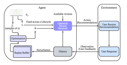
Figure 2. Deep Exploration Agent Architecture for Recommendation Systems

Algorithm 1 Deep Exploration for RS with EpiNet

1:Initialize epistemic neural network $h^{Q}_{\theta,\theta^{p}}$ and its target $h^{Q}_{\theta^{\prime},\theta^{p}}$ via EpiNet and initialize reward variance $\sigma^{2}$.

2:Initialize replay buffer $\mathcal{D}$.

3:for $t=1,2,\dots$ do $\triangleright$ Progressing over time steps

4:    Makes observation $O_{t,u}$ and computes $R_{t,u},\forall u\in\mathcal{U}_{t}$.

5:    for $u\in\mathcal{U}_{t}$ do

6:         if $z_{u}$ is not set $\lvert\rvert$ $\mathcal{A}_{t,u}=\{\text{no-op}\}$ then

7:             $z_{u}\sim P_{z}$

8:         end if

9:         $\xi_{t,u}=\textbf{extract\_interact\_features}(H_{t},u)$

10:         $\mathcal{A}_{t,u}=c(O_{t,u})$.

11:         $A_{t,u}=\arg\max_{a\in\mathcal{A}_{t,u}}h^{Q}_{\theta,\theta^{p}}(\psi_{u},\phi_{a},\xi_{t,u},z_{u})$.

12:         if $u\in\mathcal{U}_{t-1}$ then

13:             Sample $W_{t,u}\sim\mathcal{N}(0,\sigma^{2})$.

14:             Store $(\psi_{u},\phi_{A_{t-1,u}},\xi_{t-1,u},R_{t,u}+W_{t,u},\xi_{t,u},\mathcal{A}_{t,u})$ in $\mathcal{D}$.

15:         end if

16:    end for

17:    Sample data from $\mathcal{D}$ and use Equation 7 to update $\theta$.

18:end for

7. Experiments

Table 1. Average Life-Cycle Cumulative Reward across Users (DE Stands for Deep Exploration)

Algorithm	Toy	E-Commerce Train	E-Commerce Eval	Multi-User Slate Ranking Train	Multi-User Slate Ranking Eval
$\epsilon$-Greedy	$0.0\pm 0.0$	$1.07\pm 0.02$	$0.95\pm 0.07$	$94.79\pm 1.21$	$112.24\pm 2.87$
Neural TS	$0.0\pm 0.0$	$6.55\pm 1.14$	$6.37\pm 0.90$	$111.323\pm 1.34$	$119.60\pm 5.22$
Neural UCB	$0.0\pm 0.0$	$9.13\pm 0.04$	$8.035\pm 0.15$	$117.341\pm 2.03$	$119.14\pm 3.70$
Neural LinUCB	$0.0\pm 0.0$	$9.42\pm 0.13$	$8.78\pm 0.17$	$121.344\pm 4.40$	$125.50\pm 6.67$
Ensemble - DE	$0.59\pm 0.03$	$11.46\pm 0.83$	$9.82\pm 0.50$	$135.844\pm 3.62$	$152.25\pm 10.17$
EpiNet - DE	$\mathbf{0.71\pm 0.15}$	$\mathbf{16.64\pm 1.04}$	$\mathbf{13.83\pm 0.25}$	$\mathbf{147.303\pm 7.11}$	$\mathbf{178.92\pm 20.61}$

In this section, we conduct a series of experiments to demonstrate the benefits of deep exploration. We present a toy experiment following the setup in Example 2, a large-scale experiment based on an e-commerce environment, and another extensive experiment for slate ranking with parallel user streams, grounded in a game recommender system. These large-scale environments, designed by industry leaders, aim to ensure high-fidelity, model-based evaluation grounded on real-world data.

We compare deep exploration agents based on both deep ensemble and EpiNet against Q-learning agents that utilize strategies such as $\epsilon$-greedy, Neural Thompson Sampling (Neural TS) (Zhang et al., 2020), Neural UCB (Zhou et al., 2020), and Neural LinUCB (Xu et al., 2021).

In all experiments, the scaling factor of the prior network is set to 0.3. When using ensemble sampling, we set the ensemble’s cardinality to 10. In the case of EpiNet, the number of epistemic indices during optimization is set to 50, the dimension of the epistemic index is set to 10, and these indices are drawn from a standard Gaussian distribution. All agents share the same value function architecture, featuring a single hidden layer of 20 units for the toy experiment, and hidden layers of size (200, 100, 50, 25) for the remaining experiments. All experiments are executed on AWS p4d24.xlarge instances equipped with two A100 GPUs.

The results of these experiments are presented in Table 1.

7.1. SeqRec Experiment

We commence with an experiment utilizing the SeqRec environment introduced in Example 2. We’ve set $\mathcal{U}_{t}={1},\forall t$, with $\tau_{1}=10$, $b_{1}=10$, $g(1,a_{1})=0$, and $g(1,a_{2})=1$. Contrary to the case study Example 1 in Section 4.1, we do not implicitly inject prior knowledge into the agent. The action features are provided to the agent as one-hot feature vectors and each entry of the interaction feature $\xi_{t,u}\in\mathbb{R}^{10}$ is defined as:

(8) $$\xi_{t,u}[i]=\begin{cases}-1&\mbox{if }i>L_{t,u}\\ 1&\mbox{if $A_{t-L_{t}+i,u}=a_{1}$ at time step $t-L_{t}+i$}\\ 0&\mbox{otherwise}\end{cases},$$

where $L_{t,u}$ is the user’s current life-cycle length. Since there is a single user in this environment, the agent is not offered user representations. The results of the experiment, averaged over ten random seeds each with 100 life-cycles, are presented in the first column of Table 1. The results indicate that only the deep exploration agent was able to learn a reasonable policy.

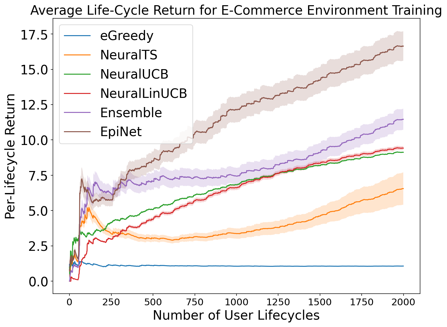
(a) Average Life-Cycle Return for High-Fidelity E-Commerce Environment through Virtual-Taobao, 200 Users Each Serving 10 Times Sequentially

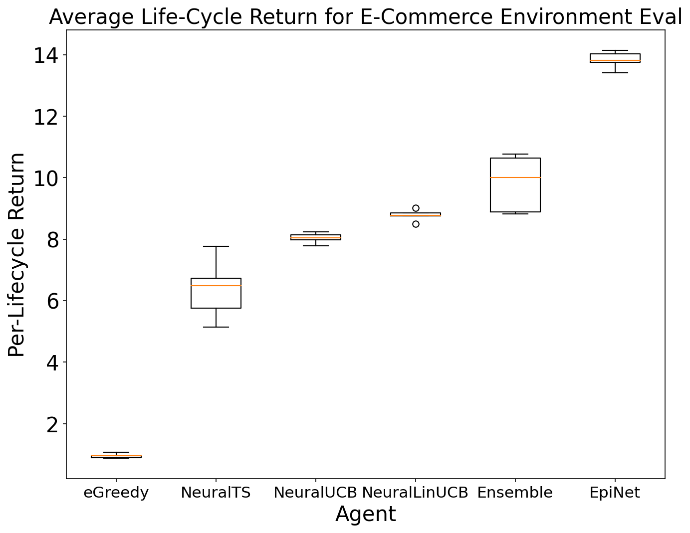
(b) Average Life-Cycle Return for High-Fidelity E-Commerce Environment with 200 Cold Start Users that Agent Has Never Seen Before

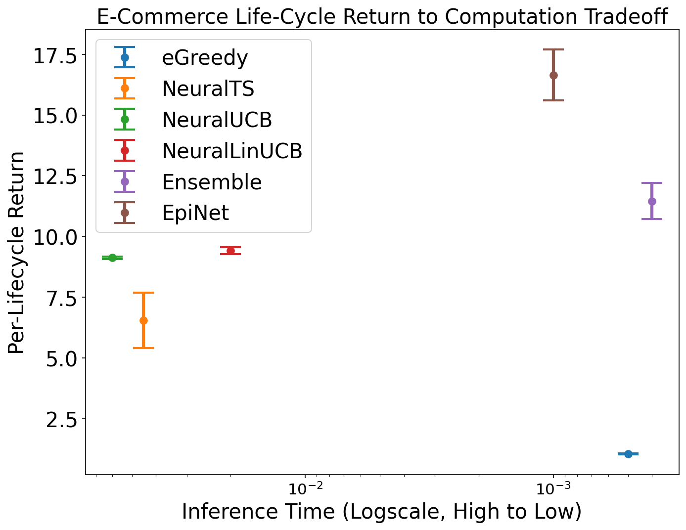
(c) Tradeoff between Life-Cycle Return and Computation for E-Commerce Experiment. Better Tradeoff towards Top Right.

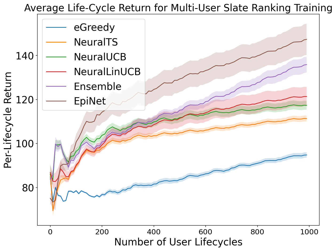
(d) Average Life-Cycle Return for High-Fidelity Multi-User Slate Ranking Environment, 100 Users Each Served 10 Times with 10-User Parallel Streams

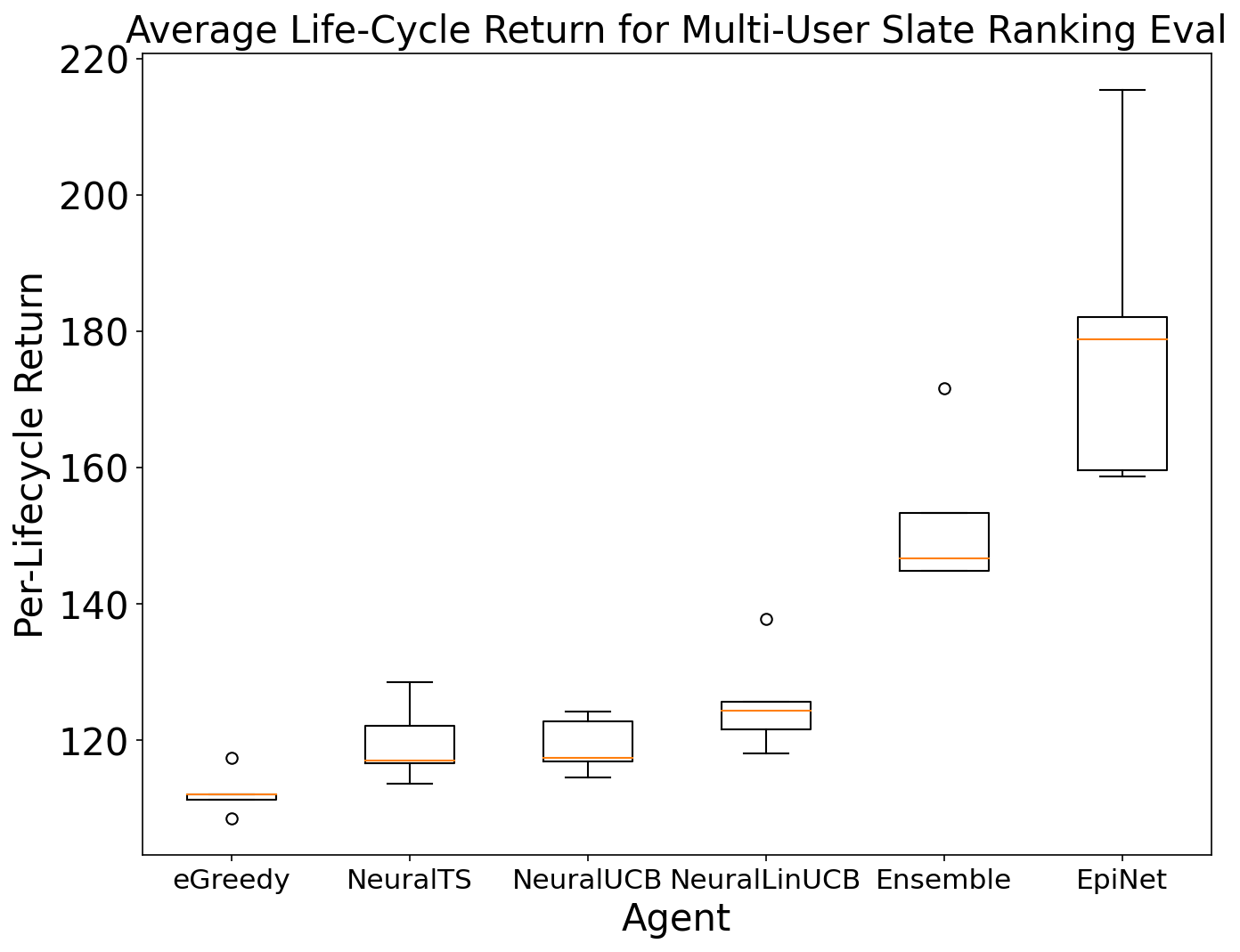
(e) Average Life-Cycle Return for High-Fidelity Multi-User Slate Ranking Environment with 100 Cold Start Users that Agent Has Never Seen Before in 10-User Parallel Streams

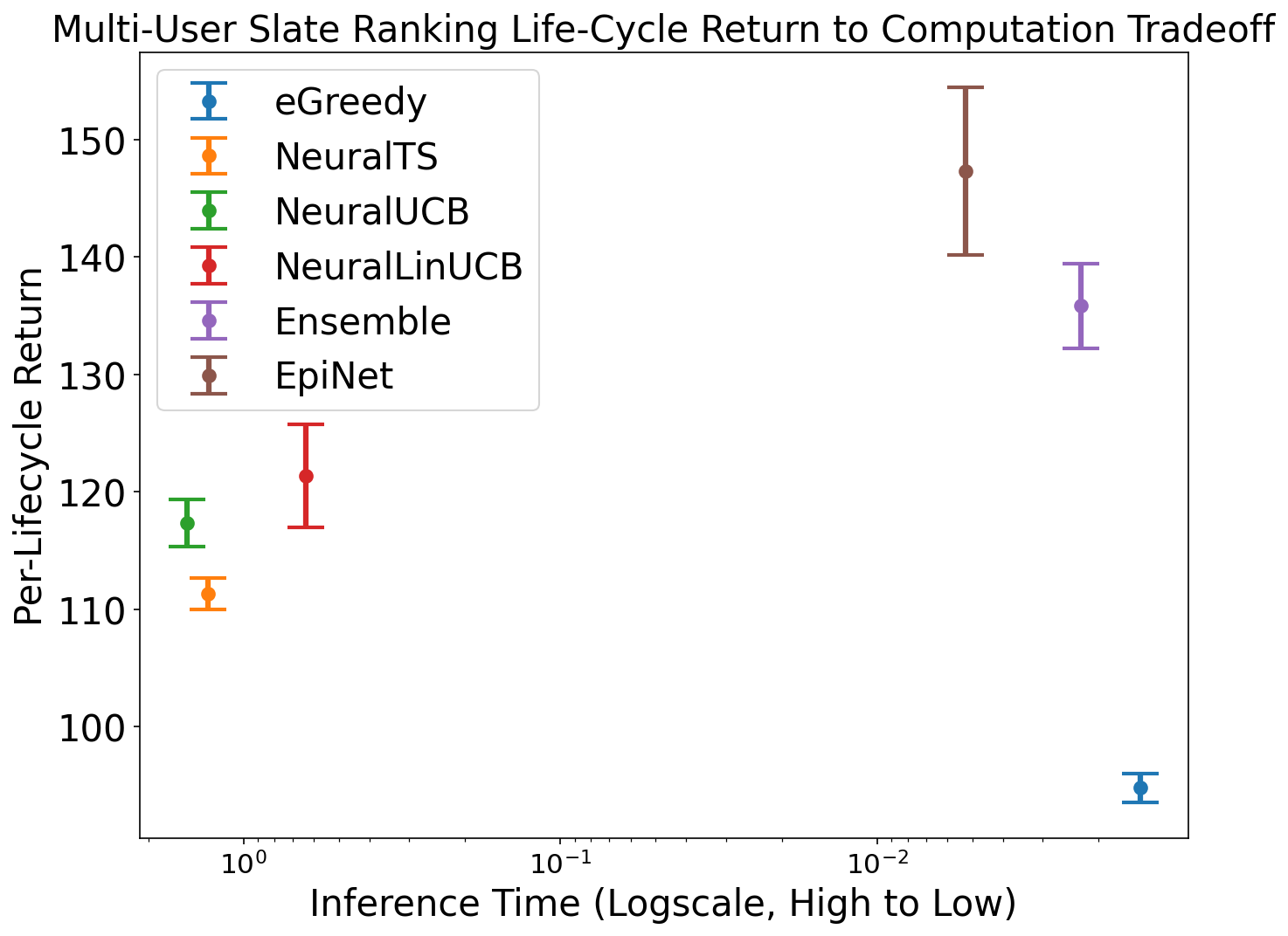
(f) Tradeoff between Life-Cycle Return and Computation for Multi-User Slate Ranking Experiment. Better Tradeoff towards Top Right.

Figure 3. Experiment Results across E-Commerce and Multi-User Slate Ranking Environments. Average life-cycle return in each of the figures above plots $\frac{1}{\lvert\mathcal{U}\rvert}\sum_{u\in\mathcal{U}}\sum_{t=1}^{T}R_{t,u}$ averaged over 30 distinct seeds, where $\mathcal{U}=\bigcup^{T}_{t=1}\mathcal{U}_{t}$ is the community of all users the agent has served and $R_{t,u}$ is the reward at time step $t$ for user $u$. Note that since the Eval set is a completely new set of users, it is normal to see evaluation’s average life-cycle return higher than training.

7.2. E-Commerce Environment

The E-Commerce environment, a classic context for Recommender Systems (RS), involves a platform suggesting items for user purchase, followed by user feedback via clicks or purchases. Virtual-Taobao (Shi et al., 2019), a model-based simulator of user behavior on one of the world’s largest E-Commerce platforms, allows us to evaluate agent performance in an online scenario with high fidelity. The environment delivers user feedback and termination via Multi-Agent Adversarial Imitation Learning (MAIL) (Song et al., 2018).

At the onset of each episode, the simulator samples a user from the user distribution via a Generative Adversarial Network (GAN) (Goodfellow et al., 2020), subsequently providing the agent with the user’s representation vector. We have arranged the environment so that at each time step, the agent is presented with 100 recommendation candidates, each with its representative features. The agent’s task is to select one to propose to the user. Additionally, the agent has access to an interaction feature vector and each user’s representative feature vector.

It is important to note that, due to the computational limitations of neural Thompson sampling and neural UCB—both of which necessitate inverting covariance matrices with the width of the neural network’s full parameter size—we only utilize the last layer’s parameter matrix and gradients for these methods in this experiment. The results of the subsequent experiments are detailed in Table 1.

Refer to Figure 3(a), which displays the results of an experiment involving 30 seeds serving 200 users, each engaged 10 life-cycles with the agent with each life-cycle happening sequentially. It is clear that both deep exploration strategies surpass other exploration methods. Notably, the deep exploration methods achieve reasonable performance much more rapidly than myopic exploration methods. Comparing the two deep exploration strategies, it is evident that EpiNet outperforms Ensemble Sampling, continually enhancing its performance throughout its interactions with users.

In addition to in-sample recommendations, we also evaluate the performance of agents trained online with 200 out-of-sample users, without any additional training. Please refer to Figure 3(b). The deep exploration methods, particularly the EpiNet-based deep exploration, significantly outperform all other candidates in out-of-sample evaluations.

Finally, the computation-performance trade-off of the algorithms is illustrated in Figure 3(c). In this graph, candidates situated towards the top right corner exhibit the optimal trade-off criteria. Here, again, the deep exploration strategies demonstrate a clear advantage.

7.3. Slate Ranking with Parallel User Streams

In an effort to extend our experimentation to a more complex and realistic setting, we utilize RL4RS (Wang et al., 2021), a real-world environment that provides parallel user streaming and slate ranking. User behavior predictions are generated via the Deep Interest Evolution Network (DIEN) (Zhou et al., 2019), and users are sampled from a real dataset with anonymized and abstract feature representations.

In this environment, the agent interacts with 10 users simultaneously, providing each user with a separate slate of recommendations. Whenever a user concludes their interactions with the agent, the environment samples a new user to maintain a constant stream of 10 active users. At each time step, the agent is presented with 284 different combinations (slates) of recommendation items as its available actions. Each slate is represented by a 128-dimensional feature vector.

Similar to the E-Commerce experiment, for the sake of computational tractability, we resort to the inversion of the last layer gradients and parameter matrix for NeuralTS and NeuralUCB. The results of the subsequent experiments are documented in Table 1.

Refer to Figure 3(d) for a 30-seed experiment serving 100 users, each with 10 life-cycles. The results illustrate that both deep exploration strategies outperform other exploration methods in this scenario. When comparing the deep exploration strategies, we observe that EpiNet slightly surpasses ensemble sampling in performance.

Similar to the e-commerce experiment previously discussed, we also evaluate our agents on an additional set of 100 out-of-sample users, as shown in Figure 3(b). Given that the experiment results originate from a distinct set of users, it is expected that the average per-user return for the evaluation set may be higher than during training. From this figure, we observe that both deep exploration methods significantly outperform the competition when applied to out-of-sample users.

Lastly, we provide a visualization of the computation-performance tradeoff in Figure 3(c). Here, it becomes evident that both deep exploration strategies lead the field in terms of this tradeoff.

8. Discussion

Deep exploration’s impact extends beyond better optimization of long-term cumulative reward. It has significant implications on data efficiency, eliminating model bias as well as data privacy.

8.1. Data Efficiency.

Reinforcement learning has a notorious sample complexity (Kakade, 2003), and sparse rewards only exacerbate this issue. As the internet and metaverse continue to expand, personalization becomes more expensive as more data must be stored for each use case. As the industry’s biggest corporations and content providers, such as Meta and Google, face shortages in data centers and computing power, data efficiency becomes crucial for RS services. Deep exploration enables content providers to identify users’ preferences with a limited number of interactions, even when feedback is sparse and delayed.

8.2. Fairness.

Fairness in gender, race and many other demographics has been one of the most important problems in machine learning research (Chouldechova and Roth, 2018; Corbett-Davies and Goel, 2018; Barocas et al., 2017). Demographic groups with a lot of data collected allow a machine learning model to generate better predictions than those with sparse data. This also applies to the RS field. Minorities enjoy less personalization because less data is collected from the group. Such phenomenon is magnified as we extend supervised learning RS algorithms to reinforcement learning and it becomes even worse in environments with sparse and delays in feedback. Deep exploration breaks the vicious cycle where the minorities get less data collected, are less personalized, then use the product less and hence get even less data collected. The low sample complexity provided by deep exploration allows for fast personalization even in environments where little data or feedback is collected.

8.3. Data Privacy.

The law pushes for a stronger regulation on data privacy and less retention of data owned by content providers. Under such regulations, content providers no longer own infinite amount of data from each user and need to make use of every piece of data possible. Such regulations have made significant impact improving the safety of user data, but meanwhile adversely impact the quality of personalization provided by content providers. Furthermore, the rise of on-device computing that further protects user privacy by owning user data locally, which further reduces the amount of data owned by content providers for personalization. Deep Exploration serves as a great tool to counter such dilemma, leveraging strategic actions to learn users’ preferences in a small number of interactions while allowing the community to improve user privacy and safety.

9. Conclusion

While deep exploration algorithms have shown great improvement over other baselines in experiments and have relatively efficient computational complexity, there is still room for future work to advance these algorithms in scalability, rigorous information seeking, and productionalization. In our experiments, we observed that deep exploration strategies tend to be slightly more expensive in both training and inference than vanilla neural networks, despite being faster than other exploration strategies. Additionally, more advanced exploration technologies, such as Information Directed Sampling (IDS) (Russo and Van Roy, 2014), could be better information-seeking strategies for deep exploration. However, IDS remains completely intractable for real-world environments as it consumes exponentially more computational resources. To develop better information-seeking deep exploration algorithms, the community needs to invest in scalable and rigorous algorithms, as well as neural network architectures that can scale such algorithms’ policy updates.

In this paper, we addressed the issue of sparse and delayed feedback in RS and explored the potential for deep exploration to improve data efficiency in personalization. We formally defined the RS problem in the context of sequential decision-making and presented real-world experimental results with our deep exploration algorithms in different high-fidelity RS environments. We demonstrated promise, through these experiments, in improving data efficiency and amplifying the rate of positive feedback in a scalable manner relative to other exploration designs in RS. We hope that the results and discussion of this paper will inspire the engineering of production systems that leverage deep exploration and show impact on real-world platforms through data-efficient personalization.

References

- (1)
- Auer et al. (2002) Peter Auer, Nicolo Cesa-Bianchi, and Paul Fischer. 2002. Finite-Time Analysis of the Multiarmed Bandit Problem. Machine Learning 47, 2-3 (2002), 235–256.
- Barocas et al. (2017) Solon Barocas, Moritz Hardt, and Arvind Narayanan. 2017. Fairness in Machine Learning. NeurIPS tutorial 1 (2017), 2.
- Bartlett et al. (2017) Peter L Bartlett, Dylan J Foster, and Matus J Telgarsky. 2017. Spectrally-Normalized Margin Bounds for Neural Networks. In Advances in Neural Information Processing Systems. 6240–6249.
- Blanda (2016) Stephanie Blanda. 2016. Online Recommender Systems–How Does a Website Know What I Want? American Mathematical Society. Retrieved October 31 (2016).
- Bouneffouf et al. (2012) Djallel Bouneffouf, Amel Bouzeghoub, and Alda Lopes Gançarski. 2012. A Contextual-Bandit Algorithm for Mobile Context-Aware Recommender System. In International Conference on Neural Information Processing. Springer, 324–331.
- Brodén et al. (2018) Björn Brodén, Mikael Hammar, Bengt J Nilsson, and Dimitris Paraschakis. 2018. Ensemble Recommendations via Thompson Sampling: an Experimental Study within E-Commerce. In 23rd international conference on intelligent user interfaces. 19–29.
- Chapelle and Li (2011) Olivier Chapelle and Lihong Li. 2011. An Empirical Evaluation of Thompson Sampling. In Advances in Neural Information Processing Systems. 2249–2257.
- Chen et al. (2019a) Minmin Chen, Alex Beutel, Paul Covington, Sagar Jain, Francois Belletti, and Ed H Chi. 2019a. Top-K Off-policy Correction for a REINFORCE Recommender System. In Proceedings of the Twelfth ACM International Conference on Web Search and Data Mining. 456–464.
- Chen et al. (2021) Minmin Chen, Yuyan Wang, Can Xu, Ya Le, Mohit Sharma, Lee Richardson, Su-Lin Wu, and Ed Chi. 2021. Values of User Exploration in Recommender Systems. In Fifteenth ACM Conference on Recommender Systems. 85–95.
- Chen et al. (2022) Minmin Chen, Can Xu, Vince Gatto, Devanshu Jain, Aviral Kumar, and Ed Chi. 2022. Off-Policy Actor-critic for Recommender Systems. In Proceedings of the 16th ACM Conference on Recommender Systems. 338–349.
- Chen et al. (2019b) Xinshi Chen, Shuang Li, Hui Li, Shaohua Jiang, Yuan Qi, and Le Song. 2019b. Generative Adversarial User Model for Reinforcement Learning based Recommendation System. In International Conference on Machine Learning. PMLR, 1052–1061.
- Cheng et al. (2016) Heng-Tze Cheng, Levent Koc, Jeremiah Harmsen, Tal Shaked, Tushar Chandra, Hrishi Aradhye, Glen Anderson, Greg Corrado, Wei Chai, Mustafa Ispir, et al. 2016. Wide & Deep Learning for Recommender Systems. In Proceedings of the 1st workshop on deep learning for recommender systems. 7–10.
- Chouldechova and Roth (2018) Alexandra Chouldechova and Aaron Roth. 2018. The Frontiers of Fairness in Machine Learning. arXiv preprint arXiv:1810.08810 (2018).
- Corbett-Davies and Goel (2018) Sam Corbett-Davies and Sharad Goel. 2018. The Measure and Mismeasure of Fairness: A Critical Review of Fair Machine Learning. arXiv preprint arXiv:1808.00023 (2018).
- Desirena et al. (2019) Gaddiel Desirena, Armando Diaz, Jalil Desirena, Ismael Moreno, and Daniel Garcia. 2019. Maximizing Customer Lifetime Value using Stacked Neural Networks: An Insurance Industry Application. In 2019 18th IEEE International Conference On Machine Learning And Applications (ICMLA). IEEE, 541–544.
- Ganganwar (2012) Vaishali Ganganwar. 2012. An Overview of Classification Algorithms for Imbalanced Datasets. International Journal of Emerging Technology and Advanced Engineering 2, 4 (2012), 42–47.
- Garivier and Cappé (2011) Aurélien Garivier and Olivier Cappé. 2011. The KL-UCB Algorithm for Bounded Stochastic Bandits and Beyond. In Proceedings of the 24th annual conference on learning theory. JMLR Workshop and Conference Proceedings, 359–376.
- Glorot and Bengio (2010) Xavier Glorot and Yoshua Bengio. 2010. Understanding the Difficulty of Training Deep Feedforward Neural Networks. In Proceedings of the Thirteenth International Conference on Artificial Intelligence and Statistics. 249–256.
- Golovin and Rahm (2004) Nick Golovin and Erhard Rahm. 2004. Reinforcement Learning Architecture for Web Recommendations. In International Conference on Information Technology: Coding and Computing, 2004. Proceedings. ITCC 2004., Vol. 1. IEEE, 398–402.
- Goodfellow et al. (2020) Ian Goodfellow, Jean Pouget-Abadie, Mehdi Mirza, Bing Xu, David Warde-Farley, Sherjil Ozair, Aaron Courville, and Yoshua Bengio. 2020. Generative Adversarial Networks. Commun. ACM 63, 11 (2020), 139–144.
- Guo et al. (2023) Hongbo Guo, Ruben Naeff, Alex Nikulkov, and Zheqing Zhu. 2023. Evaluating Online Bandit Exploration In Large-Scale Recommender System. In KDD-23 Workshop on Multi-Armed Bandits and Reinforcement Learning: Advancing Decision Making in E-Commerce and Beyond.
- He et al. (2018) Xiangnan He, Xiaoyu Du, Xiang Wang, Feng Tian, Jinhui Tang, and Tat-Seng Chua. 2018. Outer Product-based Neural Collaborative Filtering. In Proceedings of the Twenty-Seventh International Joint Conference on Artificial Intelligence. 2227–2233.
- Heyse et al. (2019) Joris Heyse, Maria Torres Vega, Femke De Backere, and Filip De Turck. 2019. Contextual Bandit Learning-Based Viewport Prediction for 360 Video. In 2019 IEEE Conference on Virtual Reality and 3D User Interfaces (VR). IEEE, 972–973.
- Hu et al. (2017) Binbin Hu, Chuan Shi, and Jian Liu. 2017. Playlist Recommendation Based on Reinforcement Learning. In International Conference on Intelligence Science. Springer, 172–182.
- Ie et al. (2019) Eugene Ie, Vihan Jain, Jing Wang, Sanmit Narvekar, Ritesh Agarwal, Rui Wu, Heng-Tze Cheng, Tushar Chandra, and Craig Boutilier. 2019. SlateQ: A Tractable Decomposition for Reinforcement Learning with Recommendation Sets. In Proceedings of the Twenty-eighth International Joint Conference on Artificial Intelligence (IJCAI-19). Macau, China, 2592–2599. See arXiv:1905.12767 for a related and expanded paper (with additional material and authors)..
- Iwata et al. (2008) Tomoharu Iwata, Kazumi Saito, and Takeshi Yamada. 2008. Recommendation Method for Improving Customer Lifetime Value. IEEE Transactions on Knowledge and Data Engineering 20, 9 (2008), 1254–1263.
- Joulani et al. (2013) Pooria Joulani, Andras Gyorgy, and Csaba Szepesvári. 2013. Online Learning under Delayed Feedback. In International Conference on Machine Learning. 1453–1461.
- Kakade (2003) Sham Machandranath Kakade. 2003. On the Sample Complexity of Reinforcement Learning. University of London, University College London (United Kingdom).
- Kamishima and Akaho (2011) Toshihiro Kamishima and Shotaro Akaho. 2011. Personalized Pricing Recommender System: Multi-Stage Epsilon-Greedy Approach. In Proceedings of the 2nd International Workshop on Information Heterogeneity and Fusion in Recommender Systems. 57–64.
- Katehakis and Veinott Jr (1987) Michael N Katehakis and Arthur F Veinott Jr. 1987. The Multi-Armed Bandit Problem: Decomposition and Computation. Mathematics of Operations Research 12, 2 (1987), 262–268.
- Ktena et al. (2019) Sofia Ira Ktena, Alykhan Tejani, Lucas Theis, Pranay Kumar Myana, Deepak Dilipkumar, Ferenc Huszár, Steven Yoo, and Wenzhe Shi. 2019. Addressing Delayed Feedback for Continuous Training with Neural Networks in CTR Prediction. In Proceedings of the 13th ACM Conference on Recommender Systems. 187–195.
- Langford and Zhang (2007) John Langford and Tong Zhang. 2007. Epoch-Greedy Algorithm for Multi-Armed Bandits with Side Information. Advances in Neural Information Processing Systems (NIPS 2007) 20 (2007), 1.
- Li et al. (2010) Lihong Li, Wei Chu, John Langford, and Robert E Schapire. 2010. A Contextual-Bandit Approach to Personalized News Article Recommendation. In Proceedings of the 19th International Conference on World Wide Web. 661–670.
- Li et al. (2011) Lihong Li, Wei Chu, John Langford, and Xuanhui Wang. 2011. Unbiased Offline Evaluation of Contextual-Bandit-Based News Article Recommendation Algorithms. In Proceedings of the Fourth ACM International Conference on Web Search and Data Mining. ACM, 297–306.
- Liu and Shih (2005) Duen-Ren Liu and Ya-Yueh Shih. 2005. Integrating AHP and Data Mining for Product Recommendation Based on Customer Lifetime Vsalue. Information & Management 42, 3 (2005), 387–400.
- Lu and Van Roy (2017) Xiuyuan Lu and Benjamin Van Roy. 2017. Ensemble Sampling. In Advances in Neural Information Processing Systems. 3258–3266.
- Mnih et al. (2015) Volodymyr Mnih, Koray Kavukcuoglu, David Silver, Andrei A Rusu, Joel Veness, Marc G Bellemare, Alex Graves, Martin Riedmiller, Andreas K Fidjeland, Georg Ostrovski, et al. 2015. Human-Level Control through Deep Reinforcement Learning. Nature 518, 7540 (2015), 529–533.
- Nakamura (2015) Atsuyoshi Nakamura. 2015. A UCB-Like Strategy of Collaborative Filtering. In Asian Conference on Machine Learning. 315–329.
- Nguyen-Thanh et al. (2019) Nhan Nguyen-Thanh, Dana Marinca, Kinda Khawam, David Rohde, Flavian Vasile, Elena Lohan, Steven Martin, and Dominique Quadri. 2019. Recommendation System-Based Upper Confidence Bound for Online Advertising. In REVEAL 2019.
- Osband et al. (2018) Ian Osband, John Aslanides, and Albin Cassirer. 2018. Randomized Prior Functions for Deep Reinforcement Learning. In Advances in Neural Information Processing Systems. 8617–8629.
- Osband et al. (2016) Ian Osband, Charles Blundell, Alexander Pritzel, and Benjamin Van Roy. 2016. Deep Exploration via Bootstrapped DQN. In Advances in Neural information processing systems.
- Osband et al. (2019) Ian Osband, Benjamin Van Roy, Daniel J Russo, and Zheng Wen. 2019. Deep Exploration via Randomized Value Functions. Journal of Machine Learning Research 20, 124 (2019), 1–62.
- Osband et al. (2021) Ian Osband, Zheng Wen, Mohammad Asghari, Morteza Ibrahimi, Xiyuan Lu, and Benjamin Van Roy. 2021. Epistemic Neural Networks. arXiv preprint arXiv:2107.08924 (2021).
- Osband et al. (2022) Ian Osband, Zhegn Wen, Seyed Mohammad Asghari, Vikranth Dwaracherla, Xiuyuan Lu, Morteza Ibrahimi, Dieterich Lawson, Botao Hao, Brendan O’Donoghue, and Benjamin Van Roy. 2022. The Neural Testbed: Evaluating Joint Predictions. In Advances in Neural Information Processing Systems.
- Qin et al. (2022) Chao Qin, Zheng Wen, Xiuyuan Lu, and Benjamin Van Roy. 2022. An Analysis of Ensemble Sampling. In Advances in Neural Information Processing Systems.
- Rojanavasu et al. (2005) Pornthep Rojanavasu, Phaitoon Srinil, and Ouen Pinngern. 2005. New Recommendation System Using Reinforcement Learning. Special Issue of the Intl. J. Computer, the Internet and Management 13, SP 3 (2005).
- Russo and Van Roy (2014) Daniel Russo and Benjamin Van Roy. 2014. Learning to Optimize via Information-Directed Sampling. In Advances in Neural Information Processing Systems. 1583–1591.
- Schafer et al. (2007) J Ben Schafer, Dan Frankowski, Jon Herlocker, and Shilad Sen. 2007. Collaborative Filtering Recommender Systems. The Adaptive Web (2007), 291–324.
- Schrittwieser et al. (2020) Julian Schrittwieser, Ioannis Antonoglou, Thomas Hubert, Karen Simonyan, Laurent Sifre, Simon Schmitt, Arthur Guez, Edward Lockhart, Demis Hassabis, Thore Graepel, et al. 2020. Mastering Atari, Go, Chess and Shogi by Planning with a Learned Model. Nature 588, 7839 (2020), 604–609.
- Shi et al. (2019) Jing-Cheng Shi, Yang Yu, Qing Da, Shi-Yong Chen, and An-Xiang Zeng. 2019. Virtual-Taobao: Virtualizing Real-World Online Retail Environment for Reinforcement Learning. In Proceedings of the AAAI Conference on Artificial Intelligence, Vol. 33. 4902–4909.
- Shih and Liu (2008) Ya-Yueh Shih and Duen-Ren Liu. 2008. Product Recommendation Approaches: Collaborative Filtering via Customer Lifetime Value and Customer Demands. Expert Systems with Applications 35, 1-2 (2008), 350–360.
- Silver et al. (2017) David Silver, Julian Schrittwieser, Karen Simonyan, Ioannis Antonoglou, Aja Huang, Arthur Guez, Thomas Hubert, Lucas Baker, Matthew Lai, Adrian Bolton, et al. 2017. Mastering the Game of Go without Human Knowledge. nature 550, 7676 (2017), 354–359.
- Song et al. (2018) Jiaming Song, Hongyu Ren, Dorsa Sadigh, and Stefano Ermon. 2018. Multi-Agent Generative Adversarial Imitation Learning. In Advances in neural information processing systems.
- Tang et al. (2019) Xueying Tang, Yunxiao Chen, Xiaoou Li, Jingchen Liu, and Zhiliang Ying. 2019. A Reinforcement Learning Approach to Personalized Learning Recommendation Systems. Brit. J. Math. Statist. Psych. 72, 1 (2019), 108–135.
- Theocharous et al. (2015) Georgios Theocharous, Philip S Thomas, and Mohammad Ghavamzadeh. 2015. Personalized Ad Recommendation Systems for Life-Time Value Optimization with Guarantees. In Twenty-Fourth International Joint Conference on Artificial Intelligence.
- Thompson (1933) William R Thompson. 1933. On the Likelihood That One Unknown Probability Exceeds Another in View of the Evidence of Two Samples. Biometrika 25, 3/4 (1933), 285–294.
- Wang et al. (2021) Kai Wang, Zhene Zou, Qilin Deng, Yue Shang, Minghao Zhao, Runze Wu, Xudong Shen, Tangjie Lyu, and Changjie Fan. 2021. RL4RS: A Real-World Benchmark for Reinforcement Learning based Recommender System. arXiv preprint arXiv:2110.11073 (2021).
- Wu et al. (2019) Chuhan Wu, Fangzhao Wu, Suyu Ge, Tao Qi, Yongfeng Huang, and Xing Xie. 2019. Neural News Recommendation with Multi-Head Self-Attention. In Proceedings of the 2019 conference on empirical methods in natural language processing and the 9th international joint conference on natural language processing (EMNLP-IJCNLP). 6389–6394.
- Xu et al. (2021) Pan Xu, Zheng Wen, Handong Zhao, and Quanquan Gu. 2021. Neural Contextual Bandits with Deep Representation and Shallow Exploration. In International Conference on Learning Representations.
- Xu et al. (2023) Ruiyang Xu, Jalaj Bhandari, Dmytro Korenkevych, Fan Liu, Yuchen He, Alex Nikulkov, and Zheqing Zhu. 2023. Optimizing Long-term Value for Auction-Based Recommender Systems via On-Policy Reinforcement Learning. In Proceedings of the 17th ACM Conference on Recommender Systems.
- Zhang et al. (2017) C Zhang, S Bengio, M Hardt, B Recht, and O Vinyals. 2017. Understanding Deep Learning Requires Rethinking Generalization Int. In Conf. on Learning Representations.
- Zhang et al. (2020) Weitong Zhang, Dongruo Zhou, Lihong Li, and Quanquan Gu. 2020. Neural Thompson Sampling. In International Conference on Learning Representations.
- Zheng et al. (2018) Guanjie Zheng, Fuzheng Zhang, Zihan Zheng, Yang Xiang, Nicholas Jing Yuan, Xing Xie, and Zhenhui Li. 2018. DRN: A Deep Reinforcement Learning Framework for News Recommendation. In Proceedings of the 2018 World Wide Web Conference on World Wide Web. International World Wide Web Conferences Steering Committee, 167–176.
- Zhou et al. (2020) Dongruo Zhou, Lihong Li, and Quanquan Gu. 2020. Neural Contextual Bandits with UCB-Based Exploration. In International Conference on Machine Learning. PMLR, 11492–11502.
- Zhou et al. (2019) Guorui Zhou, Na Mou, Ying Fan, Qi Pi, Weijie Bian, Chang Zhou, Xiaoqiang Zhu, and Kun Gai. 2019. Deep Interest Evolution Network for Click-Through Rate Prediction. In Proceedings of the AAAI conference on artificial intelligence, Vol. 33. 5941–5948.
- Zhu and Van Roy (2023) Zheqing Zhu and Benjamin Van Roy. 2023. Scalable Neural Contextual Bandit for Recommender Systems. arXiv preprint arXiv:2306.14834 (2023).