Physics-informed Convolutional Neural Networks for Temperature Field Prediction of Heat Source Layout without Labeled Data

Abstract

Recently, surrogate models based on deep learning have attracted much attention for engineering analysis and optimization. As the construction of data pairs in most engineering problems is time-consuming, data acquisition is becoming the predictive capability bottleneck of most deep surrogate models, which also exists in surrogate for thermal analysis and design. To address this issue, this paper develops a physics-informed convolutional neural network (CNN) for the thermal simulation surrogate. The network can learn a mapping from heat source layout to the steady-state temperature field without labeled data, which equals solving an entire family of partial difference equations (PDEs). To realize the physics-guided training without labeled data, we employ the heat conduction equation and finite difference method to construct the loss function. Since the solution is sensitive to boundary conditions, we properly impose hard constraints by padding in the Dirichlet and Neumann boundary conditions. In addition, the neural network architecture is well-designed to improve the prediction precision of the problem at hand, and pixel-level online hard example mining is introduced to overcome the imbalance of optimization difficulty in the computation domain. The experiments demonstrate that the proposed method can provide comparable predictions with numerical method and data-driven deep learning models. We also conduct various ablation studies to investigate the effectiveness of the network component and training methods proposed in this paper.

Keywords Physics-informed convolutional neural networks  $\cdot$ Thermal simulation  $\cdot$ Heat source layout  $\cdot$ Finite difference method  $\cdot$ Temperature field prediction

1 Introduction

With the increasing integration of electronic equipment, thermal management becomes an essential part of the electronic system design to ensure the performance and reliability of electronic components. One effective way for thermal management is to optimize the heat source layout inside the electronic device (Chen et al. (2016);Chen et al. (2017);Aslan et al. (2018))), where physics simulation plays an important role to provide temperature field computations for layout evaluation in the layout optimization loop. The physics simulation usually involves solving complex partial differential equations (PDEs). It is expensive and time-consuming in many science and engineering problems, including the thermal analysis and design, as PDEs with different design parameters must be repeatedly solved. Surrogate models, such as Gaussian processes (Lee et al. (2020)), kriging (Liu et al. (2017)), SVM regression (Moustapha et al. (2018)), and neural network (Misiulia et al. (2017)), are computationally attractive to replace the costly and repetitive physics simulations. Recently, more researches focused on the deep learning-based surrogate model benefit from the power of deep neural networks (DNNs) in solving high-dimensional and strong nonlinear problems.

This paper studies the deep surrogate model in one thermal management task named temperature field prediction of heat source layout (HSL-TFP). There exist some works on the data-driven surrogate model based on DNNs. Chen et al. (2020) modeled the temperature field prediction as an image-to-image regression task, and feature pyramid network is employed as the backbone of DNNs. Compared with numerical methods, the DNNs surrogate reduces the computation time and improves the efficiency of layout optimization. For evaluating the performance of various methods, Chen et al. (2021) summarized the HSL-TFP task benchmark from data generation, baseline models, and evaluation metrics. The data-driven deep surrogate model are also investigated in structural mechanics (Kallioras et al. (2020);Ates and Gorguluarslan (2021)), fluid mechanics (Zhu et al. (2019);Li et al. (2020a)), and materials physics (Teichert and Garikipati (2019)). As deep learning methods operate in the big data regime, amounts of training data are usually necessary to achieve reliable predictive performance. However, preparing sufficient simulation data is similarly expensive and time-consuming in such engineering and scientific field.

To reduce the cost of preparing simulation data, we investigate to incorporate physical knowledge into DNN training. Some similar research exists called physics-informed neural network (PINN), or physics-constrained neural network. Classical PINN works primarily focus on solving one PDE with specific parameters by fully-connected neural networks (FC-NNs). For example, Raissi et al. (2019) exploited PINN with the development of deep learning techniques. It leverages the capability of the deep neural network as universal function approximators and the techniques of automatic differentiation (Baydin et al. (2018)). The physics-informed loss function of PINN is constructed based on governing PDEs and is used to regularize the output for minimizing the violation of PDEs. This representive PINN has been studied in many scientific problems to solve various PDEs, including high-speed flows (Mao et al. (2020)), subsurface flows (Wang et al. (2020)), metamaterial design (Liu and Wang (2019)), power system (Misyris et al. (2020)), and heat transfer equation (Zobeiry and Humfeld (2021)).

In contrast with these studies, our work focuses on physics-informed surrogate model to learn the mapping from parametric dependence to PDE solution. It will learn an entire family of PDEs, which is more challenging than solving one instance of PDE. Therefore, we present the physics-informed surrogate model for HSL-TFP with CNN architecture. The input and output are the discrete representation of parameter and solution function, which can be treated as images. Different from automatic differentiation, the finite difference method is utilized to join the heat conduction equation into the construction of loss function. Besides, the hard constraint is imposed in the boundary by padding to avoid ill-posed solution. They collectively guide the network to minimize the violation of equations. In fact, physics-informed FC-NN methods have explored the parameterized spaces, including initial conditions, boundary conditions, and equation parameters, but FC-NN takes scalability problems reason of high-dimensional input spaces. Because of parameter sharing and local connection, CNN is more promising in large-scale and high-dimensional problems.

In physics simulation field, the CNN have been applied in discoverying underlying PDEs discovery (Long et al. (2018);Long et al. (2019)), PDEs solving (Yao et al. (2020);Zhu et al. (2019)), and surrogate model construction (Zhu et al. (2019)). Yao et al. (2020) presented that finite element method (FEA) models for PDEs is a special CNN, and FEA-Net was developed to predict the response of materials and structures. Kim et al. (2019) discretized and parameterized fluid simulation velocity fields, and a CNN-based generative model is provided to synthesize fluid simulations. In our paper, the physics-informed CNN is utilized as surrogate model in thermal simulation task. The effect of different network components is thoroughly discussed, which is helpful for researches of network structure design in this field. In addition, for the HSL-TFP task at hand, considering different optimization difficulties in the computation domain, this paper proposes pixel-level online hard example mining to weigh each position adaptively. It can drive optimizer to make more efforts into hard-optimized domain.

In conclusion, the novel contributions of our work are as follows.

1. We develop a physics-informed loss function for HSL-TFP based on heat conduction equation and finite difference method. The network can be trained by the physics-informed loss without labeled data.

2. We introduce to impose hard constraints on the Dirichlet and Neumann boundary. This will benefit the stable and fast convergence of network training.

3. A UNet-like architecture is proposed, and we emphasize discussing the performance impact of different network components.

4. To balance the optimization difficulty in the whole computation domain, we introduce the pixel-level online hard example mining for HSL-TFP. The experiments demonstrate that the proposed method can present comparable predictions with numerical and data-driven methods.

The rest of this paper is organized as follows. The description of the HSL-TFP problem is introduced in Section 2. Section 3 presents the construction of physics-informed loss function, the hard constraints on boundary conditions, the CNN-based architecture, and the pixel-level hard example mining. The results of two cases with varying difficulty are presented and discussed in Section 4. Finally, we conclude the paper in Section 5.

2 Temperature Field Prediction of Heat Source Layout (HSL-TFP)

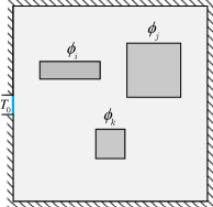
Figure 1: Schematic of the square domain with several heat source.

Assume that there is a two-dimensional rectangular heat-conducting plate with several electronic components. The plate makes heat exchange with the external environment by isothermal boundary. The components generate heat when working, and the heat is dissipated by conduction. Each component can be simplified as a heat source for this type of problem, and the heat source layout will affect the steady temperature field distribution in the whole domain. This paper expects to employ DNN to make temperature field predictions for heat source layout rapidly.

Similar to problems stated by Chen et al. (2016, 2017); Aslan et al. (2018); Chen et al. (2020, 2021), the two-dimensional conducting domain with several rectangle heat source is set as shown in Fig. 1. An isothermal boundary of length $\delta$ and temperature $T_{0}$ in the bottom exchanges heat with external circumstances. Other boundaries are adiabatic. The steady temperature field of the domain satisfies Poisson’s equation, which is expressed as follows.

$$\frac{\partial}{{\partial x}}\left({\lambda\frac{{\partial T}}{{\partial x}}}\right)+\frac{\partial}{{\partial y}}\left({\lambda\frac{{\partial T}}{{\partial y}}}\right)+\phi(x,y)=0,~{}(x,y)\in\Omega$$ (1)

where constant $\lambda$ is the thermal conductivity of the domain. $\phi(x,y)$ is the intensity distribution function, which correlates with the heat source layout. Assume that ${\phi_{i}}$ and $\Gamma_{i}$ respectively represent the intensity and distribution area of the heat source $i$, $\phi(x,y)$ can be modeled as follows

$$\phi(x,y)=\left\{{\begin{array}[]{*{20}{c}}{{\phi_{i}},}&{(x,y)\in\Gamma_{i}~{}~{}~{}i\in 1,...,n}\\ {0,}&{\rm{others}}\end{array}}\right.$$ (2)

For the problem in this paper, the equation should satisfy the Drichlet Boundary and Neumann Boundary, which are formulated as follows

$$T(x,y)={T_{0}},(x,y)~{}\in\partial\Omega_{D}$$ (3)

$$\lambda\frac{{\partial T(x,y)}}{{\partial\bm{n}}}=0,(x,y)~{}\in\partial\Omega_{N}$$ (4)

where $\Omega_{D}$ and $\Omega_{N}$ respectively denote the Drichlet and Neumann Boundary. The equation can be solved by traditional numerical methods, such as finite difference method (FDM), finite element method (FEM), and finite volume method (FVM). Consequently, traditional numerical solvers sometimes are inefficient when calling the solver frequently. In this paper, we investigate to replace the numerical solver with neural networks to make real-time temperature field predictions.

3 Physics-informed Convolutional Neural Networks for HSL-TFP

In this paper, each heat source layout corresponds to one PDE parameterized by the intensity distribution function $\phi(x,y)$. For the trained CNN, we expect the neural network takes $\phi(x,y)$ as input, and predict the two-dimentional temperature field $T$. Therefore, the network is essentially learning operators, mapping intensity distribution function to the PDE solution.

In addition, some works have shown the power of deep networks in learning operators. Motivated by the success of deep learning, Bhattacharya et al. (2021) developed a data-driven framework to describe the mapping between infinite-dimensional spaces and applied it to the elliptic PDE. Patel et al. (2021) introduced a regression framework to discover operators from molecular simulation data. Anandkumar et al. (2020) and Li et al. (2020b) proposed a graph kernel network to describe the mapping between different finite-dimensional approximations for infinite-dimensional spaces. By introducing Fourier transform, Li et al. (2020a) presented the Fourier neural operator, which is a resolution-invariant solution operator for the Navier-Stokes equation. From the universal approximation theorem, Lu et al. (2021) proposed a network, named deep operator network (DeepONet), which can make small generalization errors for deterministic and stochastic PDEs.

In contrast with these methods, the learning of deep operators is driven by physics equations in our work. For the HSL-TFP task, discrete representations of intensity distribution and solution functions are obtained by dividing mesh. These representations can be viewed as images, and CNN is employed for the image-to-image regression problem in finite dimension space. Guided by physics knowledge, CNN can learn to solve an entire family of heat conduction equations.

This section will first provide the construction of the physics-informed loss function for HSL-TFP, and the convolution layer can handily compute the loss. Then, we introduce the hard enforcement in prediction to satisfy the boundary condition. Finally, the CNN architecture based on UNet is described.

3.1 Physics-informed loss function

The Physics-informed CNN aims to learn the steady-state solutions of parametric PDEs described in Eq. 1. Let $G$ be an operator taking the intensity distribution function $\phi$, and $G(\phi)$ is solution function of the corresponding PDE. For each point $(x,y)$ in the solution $G(\phi)$, $G(\phi)(x,y)$ output the temperature, which is a real number. We consider the two-dimensional heat conduction problem for HSL-TFP, and the computation domain is set to the rectangle. Without loss of generality, the rectangle domain and boundary are described as follows.

$$D_{I}=\left\{{(x,y)|0<x<a,0<y<b}\right\}$$ (5)

$$\partial D=\{(x,y)|0\leq x\leq a,y=0{\rm{~{}or~{}}}b;x=0{\rm{~{}or~{}}}a,0\leq y\leq b\}$$ (6)

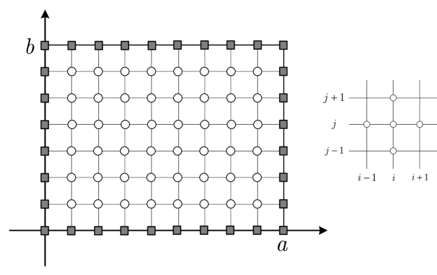
Figure 2: Illustration of mesh division in rectangle domain.

To represent the function $\phi$ and $G(\phi)$, we discretize the function domain at finite amounts of location, and the function $\phi$ and $G(\phi)$ are treated as an image. Considering the great success of CNN in image processing, we expect that the operetor $G$ can be well learned by CNN. As shown in Fig. 2, the computation domain $D$ bounded by $\partial D$ is divided into $n\times m$ rectangle mesh, and the step along the $x$-aixs and $y$-axis are $h={a\mathord{\left/{\vphantom{an}}\right.\kern-1.2pt}n}$ and $k={b\mathord{\left/{\vphantom{bm}}\right.\kern-1.2pt}m}$. Inspired by the finite difference method, the derivative terms of the solution function $G(\phi)$ could be obtained by differential approximation. Therefore, we can construct a loss function to drive the solution function $G(\phi)$ satisfy the governing equation. For inner-domain points $D_{I}$, the five-point finite difference is built by Taylor series expansion.

$$\frac{1}{{{h^{2}}}}\left[{T({x_{i}}+h,{y_{j}})-2T({x_{i}},{y_{j}})+T({x_{i}}-h,{y_{j}})}\right]=\frac{{{\partial^{2}}T}}{{\partial{x^{2}}}}+\frac{{{h^{2}}}}{{24}}\left[{\frac{{{\partial^{4}}}}{{\partial{x^{4}}}}T\left({{\xi_{1}},{y_{j}}}\right)+\frac{{{\partial^{4}}}}{{\partial{x^{4}}}}T\left({{\xi_{2}},{y_{j}}}\right)}\right]$$ (7)

where ${x_{i-1}}\leq{\xi_{1}},{\xi_{2}}\leq{x_{i+1}}$. similarly, the difference form of ${{{\partial^{2}}T}\mathord{\left/{\vphantom{{{\partial^{2}}T}{\partial{y^{2}}}}}\right.\kern-1.2pt}{\partial{y^{2}}}}$ is presented as follows.

$$\frac{1}{{{k^{2}}}}\left[{T({x_{i}},{y_{j}}+k)-2T({x_{i}},{y_{j}})+T({x_{i}},{y_{j}}-k)}\right]=\frac{{{\partial^{2}}T}}{{\partial{y^{2}}}}+\frac{{{k^{2}}}}{{24}}\left[{\frac{{{\partial^{4}}}}{{\partial{y^{4}}}}T\left({{x_{i}},{\eta_{1}}}\right)+\frac{{{\partial^{4}}}}{{\partial{y^{4}}}}T\left({{x_{i}},{\eta_{2}}}\right)}\right]$$ (8)

where ${y_{i-1}}\leq{\eta_{1}},{\eta_{2}}\leq{y_{i+1}}$. According to Eq. 7 and 8, the difference equation of Eq. 1 is obtained as follows.

$$\frac{\partial}{{\partial x}}\left({\lambda\frac{{\partial T}}{{\partial x}}}\right)+\frac{\partial}{{\partial y}}\left({\lambda\frac{{\partial T}}{{\partial y}}}\right)+\phi(x,y)$$ (9)

$$= \frac{\lambda}{{{h^{2}}}}\left[{T({x_{i}}+h,{y_{j}})-2T({x_{i}},{y_{j}})+T({x_{i}}-h,{y_{j}})}\right]$$

$$+\frac{\lambda}{{{k^{2}}}}\left[{T({x_{i}},{y_{j}}+k)-2T({x_{i}},{y_{j}})+T({x_{i}},{y_{j}}-k)}\right]+\phi(x,y)+O(h^{2}+k^{2})$$

The truncation error of the five-point finite difference is $O(h^{2}+k^{2})$. For convenience of discussion, we use $x_{i-1}$, $x_{i+1}$ to represent $({x_{i}}-h)$ and $({x_{i}}+h)$, and the same is for y-axis. For each point $T(x_{i},y_{j})$ of mesh in $D_{I}$, it should satisfy the differential equation as follows.

$$\frac{{T\left({{x_{i+1}},{y_{j}}}\right)-2T\left({{x_{i}},{y_{j}}}\right)+T({x_{i-1}},{y_{j}})}}{{{h^{2}}}}+\frac{{T\left({{x_{i}},{y_{j+1}}}\right)-2T\left({{x_{i}},{y_{j}}}\right)+T({x_{i}},{y_{j-1}})}}{{{k^{2}}}}+\frac{\phi(x,y)}{\lambda}=0$$ (10)

The loss function can be constructed based on the above difference equation. This paper makes steps $h$ and $k$ equal in mesh generation for easily calculating by a convolution kernel. Under this setting, Eq. 10 can be converted to the following form.

$$4\cdot T\left({{x_{i}},{y_{j}}}\right)-T\left({{x_{i+1}},{y_{j}}}\right)-T({x_{i-1}},{y_{j}})-T\left({{x_{i}},{y_{j+1}}}\right)-T({x_{i}},{y_{j-1}})=\frac{{h^{2}}\phi(x_{i},y_{j})}{\lambda}$$ (11)

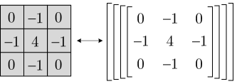
Figure 3: Laplace convolution kernel for second difference.

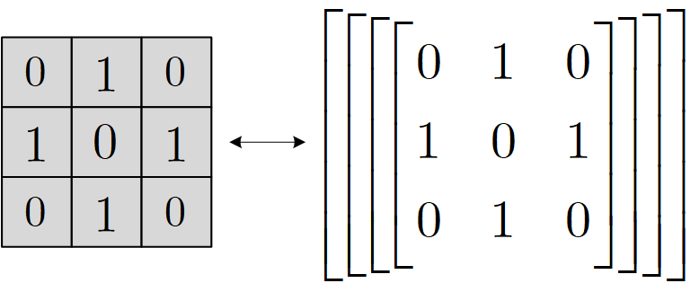
Figure 4: The convolution kernel for computing $T(x_{i},y_{j})^{\prime}$.

The temperature field $T$ is the solution $G(\phi)$ predicted by CNN. We expect each inner-domain point of $T$ to satisfy the above difference equation, and the second difference can be easily computed by the Laplace convolution kernel shown in Fig. 3. However, we discover that it is hard to train the neural network when roughly employing the Laplace convolution. Training is more efficient when the physics-informed loss function is constructed in the following form.

$${\cal L}=\frac{1}{{\left|{{D_{I}}}\right|}}\sum\limits_{(x,y)}{\left\|{T\left({{x_{i}},{y_{j}}}\right)-\frac{1}{4}T{{\left({{x_{i}},{y_{j}}}\right)}^{\prime}}}\right\|},(x,y)\in D_{I}$$ (12)

$$T(x_{i},y_{j})^{\prime}=T({x_{i+1}},{y_{j}})+T({x_{i-1}},{y_{j}})+T({x_{i}},{y_{j+1}})+T({x_{i}},{y_{j-1}})+\frac{{h^{2}}\phi(x,y)}{\lambda}$$ (13)

where $T(x_{i},y_{j})^{\prime}$ is only the intermediate variable. It can also be computed by the convolution kernel, which is shown in Fig .4. In particular, when computing $T(x_{i},y_{j})^{\prime}$, the computation graph among $T({x_{i+1}},{y_{j}})$, $T({x_{i-1}},{y_{j}})$, $T({x_{i}},{y_{j+1}})$, and $T({x_{i}},{y_{j-1}})$ need not be constructed, which avoids that the error of $T(x_{i},y_{j})^{\prime}$ affects neighboring points in back propagation. Although it is essentially derived from the difference equation of Eq. 10, this loss function formulation can significantly improve network training efficiency. In addition, the loss function can also be constructed by another difference scheme, such as the nine-point difference.

Why can the physics-informed loss function in this paper guide the neural network to learn the operator for solving an entire family of PDEs? It may be explained with the aid of the iteration method. Iterative numerical methods is an iterative algorithm to determine the solutions for the linear equations system. It is from an initial solution and bases on an iteration format to produce the approximation solution sequence. Jacobi method is a common iteration method, and the update rule for Poisson’s equation is denoted in the following form.

$$T{\left({{x_{i}},{y_{j}}}\right)^{\prime}}=\frac{{T({{x_{i+1}},{y_{j}}})+T({x_{i-1}},{y_{j}})}{+T({{x_{i}},{y_{j+1}}})+T({x_{i}},{y_{j-1}})}}{4}+\frac{{{h^{2}}}}{4\lambda}\phi({x_{i}},{y_{j}})$$ (14)

The form of the loss function is consistent with Jacobi iteration. In each back propagation, the loss function guides the network to predict the temperature field approximating the value of the next iteration. Though the network learns to solve an entire family of PDEs, not one PDE, the iteration information of other PDEs is also helpful for training because of the similarity among parametric PDEs.

3.2 Hard-contrainted boundary condition

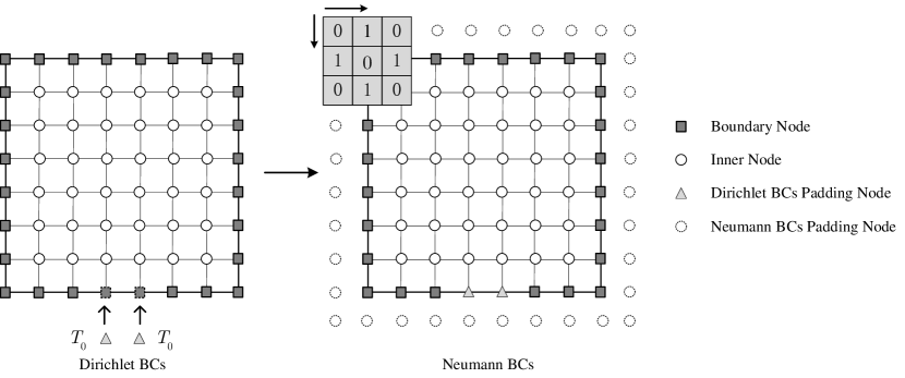
Figure 5: The illustration of enforcing hard constraint in Dirichlet and Neumann boundary.

The boundary conditions uniquely determine the solution of the steady-state problem. It is essential to add constraints on the computation domain properly. Otherwise, the PDE solving becomes ill-posed. One way is to apply soft constraints, which add penalty terms in the loss function to impel the neural network output specific values in the boundary. Since the solution is sensitive to the boundary values, the soft-constraint will negatively affect the early training when the boundary values do not fit exactly. Sun et al. (2020) introduced that soft boundary constraint will slow the convergence of PINN and devised a DNN structure to enforce the initial and boundary conditions. For CNN-based architecture, Gao et al. (2021) also studied the hard boundary condiction enforcement for solving parameterized PDE. To improve the stability and convergence speed, we also perform hard-constraint on the Dirichlet and Neumann boundary conditions for the HSL-TFP.

For the Dirichlet boundary condition defined in Eq. 3, the values in Dicichlet boundary are directly replaced by the constant value $T_{0}$, which enforces that these values do not vary during training. For the Neumann boundary condition (Eq. 4)), it is assumed that there is extra mesh $\partial\Omega^{\prime}$ surrounding the computation domain $\Omega\cup\partial\Omega$. According to the central difference formula, it should satisfy the following formulation.

$$\left\{\begin{aligned} &\lambda\frac{{{T(x_{n+1},y_{j})}-{T(x_{n-1},j)}}}{{2h}}=0,&0\leq j\leq m,\\ &\lambda\frac{{{T(x_{-1},y_{j})}-{T(x_{1},y_{j})}}}{{2h}}=0,&0\leq j\leq m,\\ &\lambda\frac{{{T(x_{i},y_{m+1})}-{T(x_{i},y_{m-1})}}}{{2h}}=0,&-1\leq i\leq n+1,\\ &\lambda\frac{{{T(x_{i},y_{-1})}-{T(x_{i},y_{1})}}}{{2h}}=0,&-1\leq i\leq n+1.\end{aligned}\right.$$ (15)

Therefore, we can enforce the padding values equal to the corresponding inner-nodes.

$$\left\{\begin{aligned} &T(x_{n+1},y_{j})=T(x_{n-1},y_{j}),&0\leq j\leq m,\\ &T(x_{-1},y_{j})=T(x_{1},y_{j}),&0\leq j\leq m,\\ &T(x_{i},y_{m+1})=T(x_{i},y_{m-1}),&-1\leq i\leq n+1,\\ &T(x_{i},y_{-1})=T(x_{i},y_{1}),&-1\leq i\leq n+1.\end{aligned}\right.$$ (16)

The schematic of enforcing hard-constrain in Dirichlet and Neumann boundary is shown in Fig. 5. Before computing the loss for gradient-based optimization, the prediction is padding with constant boundary values for Dirichlet BCs. Then the surrounding domain is expanded with inner-domain nodes for Neumann BCs. Finally, the processing map is applied to obtain the $T^{\prime}$ according to Eq. 12, and the loss is calculated without the values in Dirichlet BCs.

$$\mathcal{L}=\frac{1}{{\left|{{D_{I}}\cup{D_{N}}}\right|}}\sum\limits_{(x,y)}{\left\|{T({x_{i}},{y_{j}})-T({x_{i}},{y_{j}})^{\prime}}\right\|},({x_{i}},{y_{j}})\in({D_{I}}\cup{D_{N}})$$ (17)

3.3 CNN architecture and framework for HSL-TFP

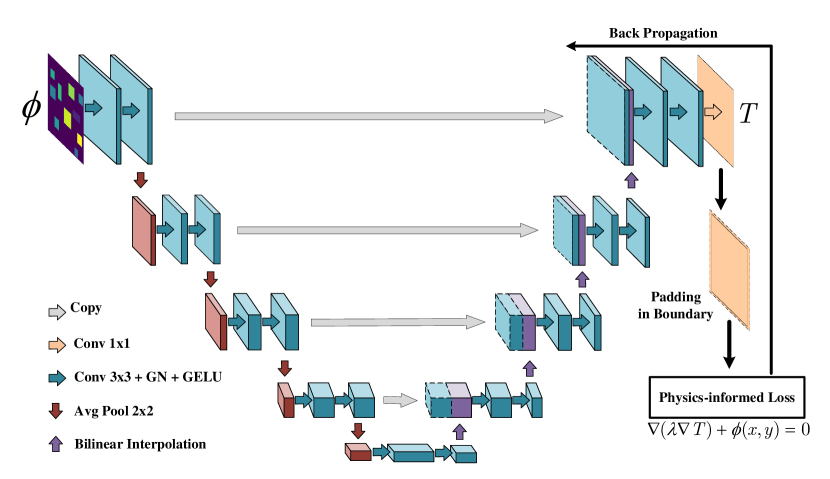
Figure 6: The pipline of physics-informed CNN for HSL-TFP. The CNN architecture is modified based on UNet for this specific task.

The inputs and outputs are both gridding data when applying the finite difference method for the two-dimensional steady-state prediction problem. When flattening the data, FC-NN will suffer from scalability problems reason of high-dimensional data space. Compared with FC-NN, CNN is superior to process image-style data. In this paper, the UNet (Ronneberger et al. (2015)) is employed as the base model, which is one excellent image-to-image CNN architecture. UNet is an encoder-decoder framework consisting of a contracting path to capture global information and an asymmetric expanding path to make high-resolution predictions. In particular, there is a skip connection in the same level of feature map for feature fusion from the encoder to decoder. Due to these special structures, UNet has achieved great success in many computer vision tasks.

Different from classification problems, the task at hand is an image-to-image regression problem. We modified UNet architecture, which is shown in Fig. 6. The inputs and outputs are respectively the discretized representation of the source term $\phi(x,y)$ and $T$ in Eq. 1. The blue arrow is the block with the 3x3 convolution layer, GroupNorm (GN), and GELU (Ronneberger et al. (2015)) activation function. We choose GN (Wu and He (2018)) because it is more stable than BacthNorm (BN) in this task. Since the values of intensity without heat source are zeros, the intensity distribution map is sparse. It changes drastically along the edge of the heat source, which is significantly different from visual images. The statistics of BN would not be exact and will harm training. In addition, GELU activation is expected to increase the ability in the nonlinear fitting. The red downward arrow is the downsampling block using average pool with 2x2 filters and stride 2. Symmetrically, the upward arrow is the 2x upsampling block with bilinear interpolation rather than the transpose convolution. Since the architecture is symmetrical, the padding of the 3x3 convolution layer is modified to 1 in contrast with original UNet, which makes the sizes of input and output under the same grid division are equal. Besides, it is worth noticing that the padding mode of convolution layers are all set to ’reflect’.

When conducting network training, we discovered large differences in the optimization difficulty of different regions. The difference equations connect the points in the physics-informed loss function, which means errors in these regions will propagate to others. To address this issue, we propose pixel-level online hard example mining (P-OHEM) to balance the optimization dynamically . The error in each pixel of the output map is represented as

$${\delta_{ij}}=\left\|{T({x_{i}},{y_{j}})-T({x_{i}},{y_{j}})^{\prime}}\right\|$$ (18)

Making $\delta$ the set of pixel-level error in map, the weight of pixel in position $(i,j)$ can be denoted as

$${w_{ij}}={\eta_{1}}+{\eta_{2}}\frac{{{\delta_{ij}}-\max(\delta)}}{{\max(\delta)+\min(\delta)}}$$ (19)

where $\eta_{1}$ and $\eta_{2}$ are the shift and scale factors. Therefore, the loss function with P-OHEM is expresses as follows.

$$\mathcal{L}=\frac{1}{{\left|{{D_{I}}\cup{D_{N}}}\right|}}\sum\limits_{(x,y)}w_{ij}{\left\|{T({x_{i}},{y_{j}})-T({x_{i}},{y_{j}})^{\prime}}\right\|},({x_{i}},{y_{j}})\in({D_{I}}\cup{D_{N}})$$ (20)

Algorithm 1 The framework of the physics-informed convolutional neural networks for HSL-TFP

Input: Intensity distribution set $\Phi$, Network parameters $\theta$, Hyperparameter $\eta_{1}$,$\eta_{2}$.
  Output: ${\theta^{*}}$

1:Randomly initialize $\theta$

2:while not done do

3:     Sample batch of intensity distribution $\Phi_{N}$ from $\Phi$

4:     Predict the temperature field $T_{N}$ with $\theta$

5:     Process boundary of $T_{N}$ with hard-constraint

6:     Calculate ${T_{N}}^{\prime}$ with Eq. 13 in no auto-grad mode

7:     Compute pixel-level weight $w_{ij}$ with Eq. 18 and Eq. 19

8:     Compute the physics-informed loss $\mathcal{L}$ with Eq. 20

9:     Update $\theta$ using $\mathcal{L}$ by auto-grad

10:end while

11:return optimized prameters ${\theta^{*}}$

For each sample, P-OHEM makes the optimizer more effort on the position with larger error, and the weight changes dynamically with the training. Benefit from this clear idea, we expect the error of each position can be uniformly decreased. Finally, the training pseudocode of the physics-informed convolutional neural networks for HSL-TFP is given in Alogorithm 1.

4 Experiment

4.1 Datasets and experimental settings

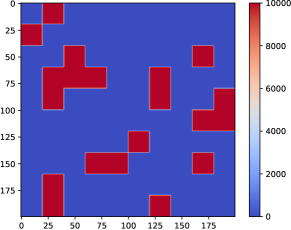
(a) layout of case 1

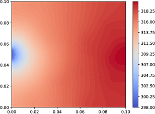
(b) temperature field of case 1

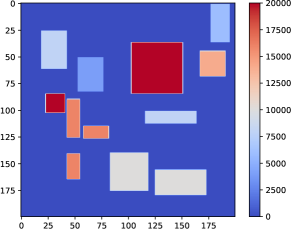
(c) layout of case 2

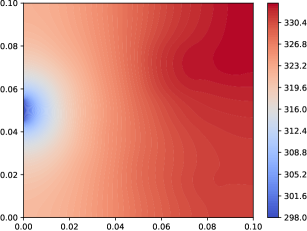
(d) temperature field of case 2

Figure 7: The layout and temperature field of two cases.

Table 1: The configuration of heat source in case 1.

Component	Size(m $\times$ m)	Intensity($w/m^{2}$)
1-20	0.01 $\times$ 0.01	10000

Table 2: The configuration of heat source in case 2.

Component	Size($m\times m$)	Intensity($w/m^{2}$)
1	0.016 $\times$ 0.012	4000
2	0.012 $\times$ 0.006	16000
3	0.018 $\times$ 0.009	6000
4	0.018 $\times$ 0.012	8000
5	0.018 $\times$ 0.018	10000
6	0.012 $\times$ 0.012	14000
7	0.018 $\times$ 0.006	16000
8	0.009 $\times$ 0.009	20000
9	0.006 $\times$ 0.024	8000
10	0.006 $\times$ 0.012	16000
11	0.012 $\times$ 0.024	10000
12	0.024 $\times$ 0.024	20000

Datasets. In this section, two cases with varying degrees of complexity are studied to demonstrate the proposed method. Firstly, the parameters of two cases are presented. The conduction domain is set to 0.1m $\times$ 0.1m square-shaped areas. One isothermal sink with a length of 0.01m is located in the middle of the left boundary, and the other is adiabatic. The thermal conductivity $\lambda$ of both domain and heat source equals $1W/(m\cdot K)$. For case 1, several square-shaped heat sources with the same setting are placed in the computation domain. For the more complex case, there are 12 rectangular heat sources with various sizes and intensities. The configurations of heat source for two cases are respectively presented in Table 1 and Table 2.

Evaluation Metrics. Chen et al. (2021) proposed a variety of metrics to evaluate the neural network performance for temperature field prediction. In this paper, we choose the following metrics, including the mean absolute error on the whole domain (MAE), the mean absolute error on the domain with components (CMAE), the maximum absolute error on the whole domain (Max-AE), and the absolute error of the maximum temperature (MT-AE).

Implementation Details. For each case, we sample 10000 heat source layout maps, and the sizes of training, validation, and test set are 9000, 1000, and 1000. The layout sampling methods are consistent with Chen et al. (2020) and Chen et al. (2021). The hyperparameters of ${\eta_{1}}$ and ${\eta_{2}}$ are set to 0 and 10, respectively. For training, we utilize Adam optimizer with the initial learning rate of 0.01, and the learning rate is adjusted by polynomial decay policy with 0.85 multiplicative factor. The batch size and the total epoch are set to 1 and 30. All models are trained on a single NVIDIA GeForce RTX 3090 GPU. The Pytorch implementation is released at https://github.com/zhaoxiaoyu1995/PI-UNet_HSL-TFP.

4.2 Prediction Performance

Table 3: The comparison of FDM computations and PI-UNet predictions.

	Training Set				Test Set
	MAE	CMAE	Max-AE	MT-AE	MAE	CMAE	Max-AE	MT-AE
Case 1	0.0098	0.0099	0.0235	0.0123	0.0108	0.0109	0.0280	0.0140
Case 2	0.0230	0.0228	0.0536	0.0277	0.0275	0.0271	0.0925	0.0336

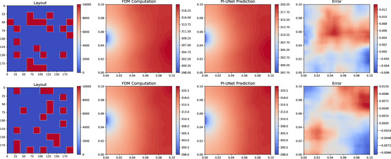
Figure 8: Prediction examples of case 1.

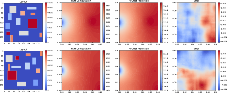
Figure 9: Prediction examples of case 2.

Numerical method is sophisticatedly to compute the temperature field by solving PDEs. In this paper, finite difference method (FDM), one of the traditional numerical methods, is chosen as the benchmark to verify the proposed method. The implementation of FDM is following Reimer and Cheviakov (2013).

As the physics-informed loss guides the CNN training without labeled data, we evaluate the network performance in the training and test sets. Our method is called as PI-UNet, and the results are presented in Table 3. First, the results show PI-UNet can make high precision predictions, as the MAE with FDM computation is less than 0.03K in two cases. Case 2 is more difficult than case 1 because all evaluation metrics are larger. Second, the difference between various evaluation metrics is small. In particular, Max-AE evaluates the maximum absolute error, which is smaller than 0.1K. It means the error between prediction and FDM computation is uniform. It is essential because unusual errors occurring in the local region will damage the prediction reliability. Finally, the small gap of evaluation metrics in the training and test set indicates that the proposed physics-informed CNN is well generalized. Fig. 8 and Fig. 9 respectively show the visual temperature field examples of prediction and FDM computation in case 1 and case 2. The network prediction is great close to the FDM computation. Since the prediction of the trained network is end-to-end and the forward propagation is very fast, the prediction by the trained network is superior in time consumption. In conclusion, the proposed method can guarantee rapid and high-precision prediction.

4.3 Comparisons with supervised learning

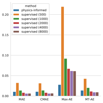
(a) case 1

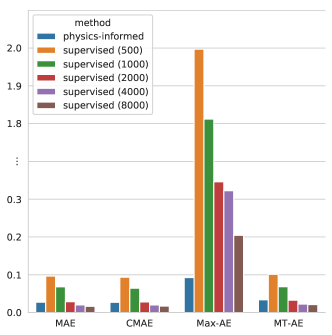
(b) case 2

Figure 10: Results of physics-informed learning and supervised learning with varying amounts of training data.

The proposed method employs physics knowledge to guide the network training. To investigate physics-informed learning and traditional supervised learning characteristics for HSL-TFP, we conduct supervised learning experiments with varying amounts of labeled data. The experimental setup is the same as physics-informed learning, except the physics-informed loss function is not applied. The number of labeled data is respectively set to 500, 1000, 2000, 4000, and 8000.

The results are compared in Fig. 10. From MAE, CMAE, and MT-AE, the precision of physics-informed learning is close to the supervised learning with 4000 labeled data. With the increase of labeled data, the model accuracy of supervised learning is higher, but there is no significant improvement. Supervised learning performs better when the labeled data is more than 4000. However, the gap between physics-informed learning and supervised learning is slight, and the precision of the proposed method meets the requirements of the application. For Max-AE, physics-informed learning is significantly lower than supervised learning. Max-AE evaluates the maximum absolute error with the FDM computation. It indicates that the supervised paradigm only learns to approximate the whole domain from labeled data, and the prediction precision in the local region is weaker than the guidance of physics. It is promising to conduct semi-supervised learning to combine the physics guidance and labeled data.

4.4 Ablation Studies

We conduct a set of ablation experiments to study the effect of the loss function, training skills, and several network components.

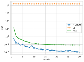
(a) case 1

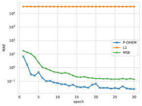
(b) case 2

Figure 11: The trend of validation MAE trained with O-OHEM, L1, and MSE loss.

Effect of P-OHEM. We perform ablation experiments to compare the performance of L1, MSE, and the proposed P-OHEM loss functions. The results of MAE evaluated in test data after each epoch can be seen in Fig. 11. When employing L1 loss, the network is unable to optimize properly, but this issue does not occur when using MSE and P-OHEM loss. Since the physics-informed loss is constructed based on PDEs and finite difference, numerical stability may be affected by the L1 loss. Result from different optimization difficulties in the computation domain, P-OHEM performs much better than MSE. In particular, since the heat dissipated from the isothermal hole and temperature changes dramatically in the domain close to the hole, decreasing the loss in these domains is more challenging. In P-OHEM, there is a larger weight for the position with a larger error, and more efforts will be made to decrease the physics-informed loss.

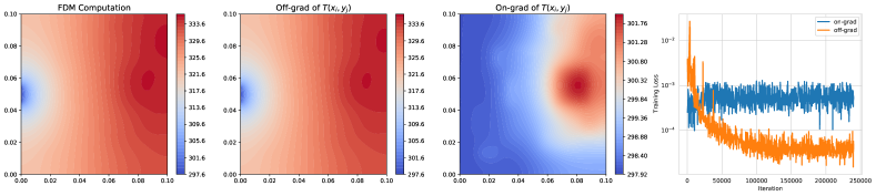
Figure 12: The effect of grad computation on or off for $T(x_{i},y_{j})^{\prime}$.

On-off of grad computation for $T(x_{i},y_{j})^{\prime}$. In the physics-informed loss Eq. 12, there is a intermediate variable $T(x_{i},y_{j})^{\prime}$. The on-off of grad computation for $T(x_{i},y_{j})^{\prime}$ has dramatically influenced the network optimization. The effect is shown in Fig. 12. When turning on the grad computation for $T(x_{i},y_{j})^{\prime}$, the network is hard to optimize, and it tends to output zero values (the prediction values are started at 298K). The intermediate variable $T(x_{i},y_{j})^{\prime}$ is constructed from surrounding predictions. When turning on the grad computation, the loss values in the current position will affect the adjacent position through back propagation, which may cause an abnormal trend of training loss.

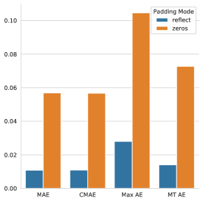
(a) case 1

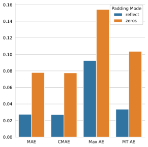
(b) case 2

Figure 13: The comparison of ’reflect’ and ’zeros’ padding mode.

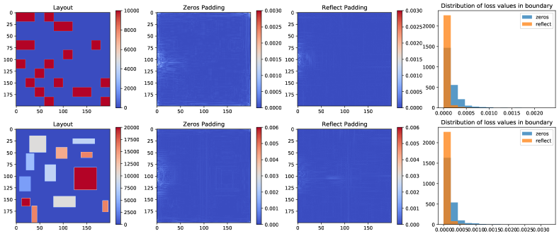
Figure 14: The distribution of physics-informed loss in ’reflect’ and ’zeros’ mode.

Padding mode. In the convolution layer with 3$\times$3 filter, the padding operator is adopted to make the input and output size unchanged. As shown in Fig. 13, ’reflect’ padding mode performs much better than ’zeros’ in all evaluation metrics. The distribution of loss values in two padding modes can be seen in Fig. 14. The loss values are relatively larger in the boundary when using ’zeros’ padding mode. Since the physics-informed loss is based on finite difference, the prediction error will diffuse from the boundary, and the prediction precision in the whole domain is reduced.

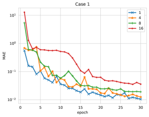
(a) case 1

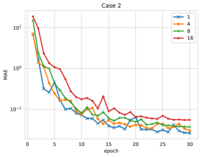
(b) case 2

Figure 15: The trend of validation MAE trained with different batch sizes. MAE is computed between the proposed method and FDM.

Batch Size. Fig. 15 shows the ablation study on the batch size. In computer vision tasks, a larger batch size usually benefits the network training. However, the results are better when the batch size is set to smaller for the task at hand. In fixed training epochs, a smaller batch size means more iteration steps, contributing to the network convergence for HSL-TFP.

Table 4: Comparison of various network components.

	Normalization	Upsampling	Activation Function	Batch Size	Train MAE	Test MAE
Case 1	GN	Bilinear	GELU	1	0.0098	0.0108
	GN	Bilinear	ReLU	1	0.0170	0.0191
	GN	Bilinear	Tanh	1	0.0198	0.0214
	BN	Bilinear	GELU	1	0.5623	0.5824
	BN	Bilinear	GELU	16	0.4701	0.4943
	IN	Bilinear	GELU	1	0.0184	0.0197
	GN	Transpose	GELU	1	0.0409	0.0421
Case 2	GN	Bilinear	GELU	1	0.0230	0.0275
	GN	Bilinear	ReLU	1	0.0464	0.0515
	GN	Bilinear	Tanh	1	0.0435	0.0491
	BN	Bilinear	GELU	1	1.1383	1.1736
	BN	Bilinear	GELU	16	0.8775	0.9358
	IN	Bilinear	GELU	1	0.0340	0.0396
	GN	Transpose	GELU	1	0.0964	0.0978

Normalization methods, upsampling methods, and activation function. We conduct ablation experiments to analyze the chooses of normalization, upsampling, and activation function. As shown in Table 4, the results of GN and IN are much better than BN, and GN is slightly better than IN. There is a great improvement of BN when turning on the training mode in evaluation. It means the statistics of BN are not incorrect in training. However, the results of BN are not notably improved with increasing the batch size to 16. For two cases, bilinear upsampling yields significantly better performance than transpose convolution. There is no clear difference in the performance of the three activation functions, but GELU is a little better. The experiments demonstrate that the combination of GN, bilinear upsampling, and GELU is most effective.

5 Conclusions

This paper investigates the physics-informed convolutional neural networks for temperature field prediction of heat source layout. First, we construct a physics-informed loss inspired by physics equations and the finite difference method. The loss guides the network to learn an operator mapping from intensity distribution function to solution function without simulation data. Furthermore, we study to impose hard constrain on the Dirichlet and Neumann boundary to speed the network convergence. Finally, we develop a well-designed architecture based on UNet for the HSL-TFP task, and pixel-level online hard example mining is proposed to balance different optimization difficulties in the computation domain. For two HSL-TFP tasks, the experiments demonstrate that the proposed method can make high-precision temperature field predictions comparable to the numerical method and data-driven models. The trained network can directly output the solution of HSL-TFP without solving PDE. It can be employed as a surrogate model to assist the layout optimization benefit from rapid and high-precision prediction.

Similar to the steady-state temperature field prediction, the developed methods can be generalized to other physics problems, employing networks to solve parameterized PDEs, such as elastic mechanics, fluid mechanics, and electromagnetism. Furthermore, it is promising to investigate the methods in irregular computation domain and large-scale mesh. In some applications, data-driven method is more effective. Combining physics knowledge and labeled data is valuable to perform model verification, semi-supervised learning, and transfer learning.

References

- Anandkumar et al. (2020) Anandkumar, A., Azizzadenesheli, K., Bhattacharya, K., Kovachki, N., Li, Z., Liu, B., Stuart, A., 2020. Neural operator: Graph kernel network for partial differential equations, in: ICLR 2020 Workshop on Integration of Deep Neural Models and Differential Equations.
- Aslan et al. (2018) Aslan, Y., Puskely, J., Yarovoy, A., 2018. Heat source layout optimization for two-dimensional heat conduction using iterative reweighted l1-norm convex minimization. International Journal of Heat and Mass Transfer 122, 432–441. doi:10.1016/j.ijheatmasstransfer.2018.02.001.
- Ates and Gorguluarslan (2021) Ates, G.C., Gorguluarslan, R.M., 2021. Two-stage convolutional encoder-decoder network to improve the performance and reliability of deep learning models for topology optimization. Structural and Multidisciplinary Optimization 63, 1927–1950.
- Baydin et al. (2018) Baydin, A.G., Pearlmutter, B.A., Radul, A.A., Siskind, J.M., 2018. Automatic differentiation in machine learning: a survey. Journal of machine learning research 18.
- Bhattacharya et al. (2021) Bhattacharya, K., Hosseini, B., Kovachki, N.B., Stuart, A.M., 2021. Model reduction and neural networks for parametric pdes. The SMAI journal of computational mathematics 7, 121–157.
- Chen et al. (2016) Chen, K., Wang, S., Song, M., 2016. Optimization of heat source distribution for two-dimensional heat conduction using bionic method. International Journal of Heat and Mass Transfer 93, 108–117. doi:10.1016/j.ijheatmasstransfer.2015.09.041.
- Chen et al. (2017) Chen, K., Xing, J., Wang, S., Song, M., 2017. Heat source layout optimization in two-dimensional heat conduction using simulated annealing method. International Journal of Heat and Mass Transfer 108, 210–219. doi:10.1016/j.ijheatmasstransfer.2016.12.007.
- Chen et al. (2020) Chen, X., Chen, X., Zhou, W., Zhang, J., Yao, W., 2020. The heat source layout optimization using deep learning surrogate modeling. Structural and Multidisciplinary Optimization 62, 3127–3148.
- Chen et al. (2021) Chen, X., Zhao, X., Gong, Z., Zhang, J., Zhou, W., Chen, X., Yao, W., 2021. A deep neural network surrogate modeling benchmark for temperature field prediction of heat source layout. arXiv preprint arXiv:2103.11177 .
- Gao et al. (2021) Gao, H., Sun, L., Wang, J.X., 2021. Phygeonet: physics-informed geometry-adaptive convolutional neural networks for solving parameterized steady-state pdes on irregular domain. Journal of Computational Physics 428, 110079.
- Kallioras et al. (2020) Kallioras, N.A., Kazakis, G., Lagaros, N.D., 2020. Accelerated topology optimization by means of deep learning. Structural and Multidisciplinary Optimization 62, 1185–1212.
- Kim et al. (2019) Kim, B., Azevedo, V.C., Thuerey, N., Kim, T., Gross, M., Solenthaler, B., 2019. Deep fluids: A generative network for parameterized fluid simulations, in: Computer Graphics Forum, Wiley Online Library. pp. 59–70.
- Lee et al. (2020) Lee, T., Bilionis, I., Tepole, A.B., 2020. Propagation of uncertainty in the mechanical and biological response of growing tissues using multi-fidelity gaussian process regression. Computer methods in applied mechanics and engineering 359, 112724.
- Li et al. (2020a) Li, Z., Kovachki, N., Azizzadenesheli, K., Liu, B., Bhattacharya, K., Stuart, A., Anandkumar, A., 2020a. Fourier neural operator for parametric partial differential equations. arXiv preprint arXiv:2010.08895 .
- Li et al. (2020b) Li, Z., Kovachki, N., Azizzadenesheli, K., Liu, B., Bhattacharya, K., Stuart, A., Anandkumar, A., 2020b. Multipole graph neural operator for parametric partial differential equations. arXiv preprint arXiv:2006.09535 .
- Liu and Wang (2019) Liu, D., Wang, Y., 2019. Multi-fidelity physics-constrained neural network and its application in materials modeling. Journal of Mechanical Design 141.
- Liu et al. (2017) Liu, X., Wu, Y., Wang, B., Ding, J., Jie, H., 2017. An adaptive local range sampling method for reliability-based design optimization using support vector machine and kriging model. Structural and Multidisciplinary Optimization 55, 2285–2304.
- Long et al. (2019) Long, Z., Lu, Y., Dong, B., 2019. Pde-net 2.0: Learning pdes from data with a numeric-symbolic hybrid deep network. Journal of Computational Physics 399, 108925.
- Long et al. (2018) Long, Z., Lu, Y., Ma, X., Dong, B., 2018. Pde-net: Learning pdes from data, in: International Conference on Machine Learning, PMLR. pp. 3208–3216.
- Lu et al. (2021) Lu, L., Jin, P., Pang, G., Zhang, Z., Karniadakis, G.E., 2021. Learning nonlinear operators via deeponet based on the universal approximation theorem of operators. Nature Machine Intelligence 3, 218–229.
- Mao et al. (2020) Mao, Z., Jagtap, A.D., Karniadakis, G.E., 2020. Physics-informed neural networks for high-speed flows. Computer Methods in Applied Mechanics and Engineering 360, 112789.
- Misiulia et al. (2017) Misiulia, D., Elsayed, K., Andersson, A.G., 2017. Geometry optimization of a deswirler for cyclone separator in terms of pressure drop using cfd and artificial neural network. Separation and Purification Technology 185, 10–23.
- Misyris et al. (2020) Misyris, G.S., Venzke, A., Chatzivasileiadis, S., 2020. Physics-informed neural networks for power systems, in: 2020 IEEE Power & Energy Society General Meeting (PESGM), IEEE. pp. 1–5.
- Moustapha et al. (2018) Moustapha, M., Bourinet, J.M., Guillaume, B., Sudret, B., 2018. Comparative study of kriging and support vector regression for structural engineering applications. ASCE-ASME Journal of Risk and Uncertainty in Engineering Systems, Part A: Civil Engineering 4, 04018005.
- Patel et al. (2021) Patel, R.G., Trask, N.A., Wood, M.A., Cyr, E.C., 2021. A physics-informed operator regression framework for extracting data-driven continuum models. Computer Methods in Applied Mechanics and Engineering 373, 113500.
- Raissi et al. (2019) Raissi, M., Perdikaris, P., Karniadakis, G.E., 2019. Physics-informed neural networks: A deep learning framework for solving forward and inverse problems involving nonlinear partial differential equations. Journal of Computational Physics 378, 686–707.
- Reimer and Cheviakov (2013) Reimer, A.S., Cheviakov, A.F., 2013. A matlab-based finite-difference solver for the poisson problem with mixed dirichlet–neumann boundary conditions. Computer Physics Communications 184, 783–798.
- Ronneberger et al. (2015) Ronneberger, O., Fischer, P., Brox, T., 2015. U-net: Convolutional networks for biomedical image segmentation, in: International Conference on Medical image computing and computer-assisted intervention, Springer. pp. 234–241.
- Sun et al. (2020) Sun, L., Gao, H., Pan, S., Wang, J.X., 2020. Surrogate modeling for fluid flows based on physics-constrained deep learning without simulation data. Computer Methods in Applied Mechanics and Engineering 361, 112732.
- Teichert and Garikipati (2019) Teichert, G.H., Garikipati, K., 2019. Machine learning materials physics: Surrogate optimization and multi-fidelity algorithms predict precipitate morphology in an alternative to phase field dynamics. Computer Methods in Applied Mechanics and Engineering 344, 666–693.
- Wang et al. (2020) Wang, N., Zhang, D., Chang, H., Li, H., 2020. Deep learning of subsurface flow via theory-guided neural network. Journal of Hydrology 584, 124700.
- Wu and He (2018) Wu, Y., He, K., 2018. Group normalization, in: Proceedings of the European conference on computer vision (ECCV), pp. 3–19.
- Yao et al. (2020) Yao, H., Gao, Y., Liu, Y., 2020. Fea-net: A physics-guided data-driven model for efficient mechanical response prediction. Computer Methods in Applied Mechanics and Engineering 363, 112892.
- Zhu et al. (2019) Zhu, Y., Zabaras, N., Koutsourelakis, P.S., Perdikaris, P., 2019. Physics-constrained deep learning for high-dimensional surrogate modeling and uncertainty quantification without labeled data. Journal of Computational Physics 394, 56–81.
- Zobeiry and Humfeld (2021) Zobeiry, N., Humfeld, K.D., 2021. A physics-informed machine learning approach for solving heat transfer equation in advanced manufacturing and engineering applications. Engineering Applications of Artificial Intelligence 101, 104232.