A new Lagrange multiplier approach for constructing structure-preserving schemes, II. bound preserving

Abstract

In the second part of this series, we use the Lagrange multiplier approach proposed in the first part [6] to construct efficient and accurate bound and/or mass preserving schemes for a class of semi-linear and quasi-linear parabolic equations. We establish stability results under a general setting, and carry out an error analysis for a second-order bound preserving scheme with a hybrid spectral discretization in space. We apply our approach to several typical PDEs which preserve bound and/or mass, also present ample numerical results to validate our approach.

65M70; 65K15; 65N22

1 Introduction

Solutions of partial differential equations (PDEs) arising from sciences and engineering applications are often required to be positive or to remain in a bounded interval. It is beneficial, and often necessary, that their numerical approximations preserve the positivity or bound at the discrete level. In recent years, a large effort has been devoted to construct bound preserving schemes for various problems.

In the first part of this series [6], we constructed a class of positivity preserving schemes using a new Lagrange multiplier approach. A main objective of this paper is to extend the approach in [6] to construct bound preserving schemes for a class of nonlinear PDEs in the following form:

(1.1) $$u_{t}+\mathcal{L}u+\mathcal{N}(u)=0,$$

with suitable initial and boundary conditions, where $\mathcal{L}$ is a linear or nonlinear non-negative operator and $\mathcal{N}(u)$ is a semi-linear or quasi-linear operator. We assume that the solution of (1.1) is bound preserving, i.e., $a\leq u(\boldsymbol{x},0)\leq b$ for all $\boldsymbol{x}\in\Omega$, then $a\leq u(\boldsymbol{x},t)\leq b$ for all $(\boldsymbol{x},t)\in\Omega\times(0,T)$.

There are a large body of work devoted to construct positivity/bound preserving schemes for (1.1). We refer to the first part of this series [6] (and the references therein) for a summary of existing approaches for constructing positivity/bound preserving schemes. In particular, large efforts have been devoted to construct spatial discretization for (1.1) such that the resulting numerical scheme satisfies a discrete maximum principle (cf., for instance, [11, 7, 8, 10, 21, 27, 20, 19], and the review paper in [12] for a up-to-date summary in this regard).

Given a generic spatial discretization of (1.1):

(1.2) $$\begin{split}\partial_{t}u_{h}+\mathcal{L}_{h}u_{h}+\mathcal{N}_{h}(u_{h})=0,\end{split}$$

where $u_{h}$ is in certain finite dimensional approximation space $X_{h}$ and $\mathcal{L}_{h}$ is a certain approximation of $\mathcal{L}$. In general, the solution $u_{h}$, if it exists, may not be bound preserving. Oftentimes, (1.2) may not be well posed if the values of $u_{h}$ go outside of $[a,b]$. For example, a direct finite elements or spectral approximation to the Allen-Cahn or Cahn-Hilliard equation with logarithmic potential may not be well posed. Instead of using special spatial discretizations which satisfy a discrete maximum principle, we aim to develop a bound preserving approach which can be used for a large class of spatial discretizations. To preserve positivity, it suffices to introduce a Lagrange multiplier $\lambda_{h}$. But to preserve bound, we need to introduce an additional quadratic function $g(u)=(b-u)(u-a)$, and consider the following expanded system with a Lagrange multiplier $\lambda_{h}$:

(1.3) $$\begin{split}&\partial_{t}u_{h}+\mathcal{L}_{h}u_{h}+\mathcal{N}_{h}(u_{h})=\lambda_{h}g^{\prime}(u_{h}),\\ &\lambda_{h}\geq 0,\;g(u_{h})\geq 0,\;\lambda_{h}g(u_{h})=0.\end{split}$$

The second equation in (1.3) represents the well-known KKT conditions [17, 14, 16, 2] for constrained minimization. The problem (1.3) can be viewed as an approximation to (1.1), it can also be viewed as a discrete problem without a background PDE, e.g., coming from a discrete constrained minimization problem.

Existing approaches for (1.3) usually start with an implicit time discretization scheme so that the nonlinear system at each time step can still be interpreted as a constrained minimization, then apply a suitable iterative procedure (cf. [26]). As in [6], we shall use a different approach which decouples the computation of Lagrange multiplier $\lambda_{h}$ from that of $u_{h}$, leading to a much more efficient algorithm.

We recall that for positivity preserving, we simply use $g(u_{h})=u_{h}$ in the above formulation. However, for bound preserving, the nonlinear nature of $g(u_{h})$ makes it much harder to prove stability in norms involving derivatives, and mass conservation whenever is necessary. On the other hand, since the numerical solutions remain to be bounded by construction, this allows us to derive more precise stability results, which in turns enable us to obtain optimal error estimates for both semi-linear and quasi-linear PDEs. More precisely, the bound preserving schemes that we construct based on the operator splitting approach enjoy all advantages of the positivity preserving schemes in [6], and furthermore, thanks to the bound preserving property, it allows us to prove a more precise stability result (see Theorem 3.1) and to establish rigorous error estimates for a class of semi-linear and quasi-linear dissipative equations (see Theorem 4.1).

We would like to point out that the schemes constructed in this paper include the usual cut-off approach [22] as a special case. Therefore, our presentation provides an alternative interpretation of the cur-off approach, and allows us to construct new cut-off implicit-explicit (IMEX) schemes with mass conservation.

To validate our schemes, we apply our new schemes to a variety of problems with bound preserving solutions, including the Allen-Cahn [1] and Cahn-Hilliard [3] equations and a class of Fokker-Planck equations [23].

The remainder of the paper is organized as follows. In Section 2, we construct bound preserving schemes for general nonlinear systems (1.1) using the Lagrange multiplier approach. For problems which also conserve mass, we modify our bound preserving schemes so that they also conserve mass. In Section 3, we restrict ourselves to second-order parabolic type equations, and establish a stability result for, as an example, the second-order scheme with mass conservation. In Section 4, we consider a hybrid spectral method as an example to carry out an error analysis for a fully discretized second-order scheme. In Section 5, we describe applications of our schemes to several typical PDEs with bound and/or mass preserving properties. In Section 6, we present some numerical simulations to validate the accuracy and robustness of our schemes. And we conclude with some remarks in the final section.

2 Bound-preserving schemes

We construct in this section efficient bound preserving schemes for solving (1.3). The key is to adopt an operator splitting approach in which a standard scheme, which is not bound preserving, is used in the first step, while in the second step, the solution is made bound preserving with a simple yet consistent procedure.

We shall first describe a generic spatial discretization with nodal Lagrangian basis functions, followed by time discretization without and with mass conservation.

Let $\Sigma_{h}$ be a set of mesh points or collocation points in $\bar{\Omega}$. Note that $\Sigma_{h}$ should not include the points at the part of the boundary where a Dirichlet (or essential) boundary condition is prescribed, while it should include the points at the part of the boundary where a Neumann or mixed (or non-essential) boundary condition is prescribed.

We assume that (1.3) is satisfied point-wisely as follows:

(2.4) $$\begin{split}&\partial_{t}u_{h}(\boldsymbol{z},t)+\mathcal{L}_{h}u_{h}+\mathcal{N}_{h}(u_{h})=\lambda_{h}(\boldsymbol{z},t)g^{\prime}(u_{h}),\quad\forall{\boldsymbol{z}}\in\Sigma_{h},\\ &\lambda_{h}(\boldsymbol{z},t)\geq 0,\;g(u_{h}(\boldsymbol{z},t))\geq 0,\;\lambda_{h}(\boldsymbol{z},t)g(u_{h}(\boldsymbol{z},t))=0,\quad\forall{\boldsymbol{z}}\in\Sigma_{h},\end{split}$$

with the Dirichlet boundary condition to be satisfied point-wisely if the original problem includes Dirichlet boundary condition at part or all of boundary. The above scheme includes finite difference schemes, collocation schemes, or Galerkin type spatial discretization with a Lagrangian basis.

Denote $\delta t$ the time step, and $t^{n}=n\delta t$ for $n=0,1,2,\cdots,\frac{T}{\delta t}$ where $T$ is the final computational time. Our schemes consist of two steps: in the first step, we use a generic time discretization, which can be implicit, explicit or implicit-explicit, to find an intermediate solution $\tilde{u}_{h}^{n+1}$ which is usually not bound preserving; then we introduce a Lagrange multiplier $\lambda_{h}^{n+1}(\boldsymbol{z})$ to determine a bound preserving ${u}_{h}^{n+1}$, which is a correction to $\tilde{u}_{h}^{n+1}$. We shall first construct bound preserving schemes which do not necessarily preserve mass, then we introduce a simple modification which allows us to construct bound preserving schemes which can also preserve mass.

For the sake of clarity, we shall restrict ourselves to constructed schemes based on the implicit-explicit (IMEX) type time discretization since they are most commonly used for parabolic type systems. It is straightforward to extend the approach below to schemes based on other types of time discretization.

2.1 A class of multistep IMEX schemes

We construct below $k$-th order bound-preserving schemes for (2.4) based on backward difference formula (BDF) for the time derivative and Adams-Bashforth extrapolation by using a predictor-corrector approach.

In order to describe the scheme, we define a sequence $\{\alpha_{k}\}$, and with a slight abuse of notation. For any function $v$, we use $A_{k}(v^{n})$ and $B_{k-1}(v^{n})$ to denote two operators depending on $(v^{n},\cdots,v^{n-k+1})$ as follows:

$k=1$:

(2.5) $$\alpha_{1}=1,\quad A_{1}(v^{n})=v^{n},\quad B_{0}(v^{n})=0;$$

$k=2$:

(2.6) $$\alpha_{2}=\frac{3}{2},\quad A_{2}(v^{n})=2v^{n}-\frac{1}{2}v^{n-1},\quad B_{1}(v^{n})=v^{n};$$

$k=3$:

(2.7) $$\begin{split}\alpha_{3}=\frac{11}{6},&\quad A_{3}(v^{n})=3v^{n}-\frac{3}{2}v^{n-1}+\frac{1}{3}v^{n-2},\\ &B_{2}(v^{n})=2v^{n}-v^{n-1}.\end{split}$$

The formula for $k=4,5,6$ can be derived similarly with Taylor expansions.

We assume that $u_{h}^{j},j=0,1,\cdots,k-1$ are properly initialized. Then

Step 1: (Predictor) solve $\tilde{u}_{h}^{n+1}$ from

(2.8) $$\begin{split}&\frac{\alpha_{k}\tilde{u}_{h}^{n+1}(\boldsymbol{z})-A_{k}(u_{h}^{n}(\boldsymbol{z}))}{\delta t}+\mathcal{L}_{h}\tilde{u}_{h}^{n+1}(\boldsymbol{z})+\mathcal{N}_{h}(B_{k}(u_{h}^{n}(\boldsymbol{z})))=B_{k-1}(\lambda_{h}^{n}g^{\prime}(u_{h}^{n}(\boldsymbol{z}))),\quad\forall{\boldsymbol{z}}\in\Sigma_{h};\end{split}$$

Step 2: (Corrector) solve $u_{h}^{n+1}$ and $\lambda_{h}^{n+1}$ from

(2.9a) $$\frac{\alpha_{k}(u_{h}^{n+1}(\boldsymbol{z})-\tilde{u}_{h}^{n+1}(\boldsymbol{z}))}{\delta t}=\lambda_{h}^{n+1}(\boldsymbol{z})g^{\prime}(u_{h}^{n+1}(\boldsymbol{z}))-B_{k-1}(\lambda_{h}^{n}(\boldsymbol{z})g^{\prime}(u_{h}^{n}(\boldsymbol{z}))),$$

(2.9b) $$g(u_{h}^{n+1}(\boldsymbol{z}))\geq 0,\;\lambda_{h}^{n+1}(\boldsymbol{z})\geq 0,\;\lambda_{h}^{n+1}(\boldsymbol{z})g(u_{h}^{n+1}(\boldsymbol{z}))=0,\quad\forall{\boldsymbol{z}}\in\Sigma_{h}.$$

The second step can be solved point-wisely as follows. We denote

(2.10) $$\eta_{h}^{n+1}:=-\frac{\delta t}{\alpha_{k}}B_{k-1}(\lambda_{h}^{n}g^{\prime}(u_{h}^{n})),$$

and rewrite (2.9a) as

$$\frac{\alpha_{k}(u_{h}^{n+1}(\boldsymbol{z})-(\tilde{u}_{h}^{n+1}(\boldsymbol{z})+\eta^{n+1}_{h}(\boldsymbol{z})))}{\delta t}=\lambda_{h}^{n+1}(\boldsymbol{z})g^{\prime}(u_{h}^{n+1}(\boldsymbol{z})).$$

We find from the above and (2.9b) that

(2.11) $$\begin{split}&(u_{h}^{n+1}(\boldsymbol{z}),\lambda_{h}^{n+1}(\boldsymbol{z}))=\left\{\begin{array}[]{rcl}(\tilde{u}_{h}^{n+1}(\boldsymbol{z})+\eta^{n+1}_{h}(\boldsymbol{z}),0)&&{\mbox{if}\quad a<\tilde{u}_{h}^{n+1}(\boldsymbol{z})}+\eta^{n+1}_{h}(\boldsymbol{z})<b\\ (a,\frac{a-(\tilde{u}_{h}^{n+1}(\boldsymbol{z})+\eta^{n+1}_{h}(\boldsymbol{z}))}{\frac{\delta t}{\alpha_{k}}g^{\prime}(a)})&&{\mbox{if}\quad\tilde{u}_{h}^{n+1}(\boldsymbol{z})+\eta^{n+1}_{h}(\boldsymbol{z})\leq a}\\ (b,\frac{b-(\tilde{u}_{h}^{n+1}(\boldsymbol{z})+\eta^{n+1}_{h}(\boldsymbol{z}))}{\frac{\delta t}{\alpha_{k}}g^{\prime}(b)})&&{\mbox{if}\quad\tilde{u}_{h}^{n+1}(\boldsymbol{z})}+\eta^{n+1}_{h}(\boldsymbol{z})\geq b\end{array}\right.,\;\forall\boldsymbol{z}\in\Sigma_{h}.\end{split}$$

Remark 2.1.

It is obvious that the above scheme is a $k$-th order approximation to (2.4). We would like to point out that it is also a $k$-th order (in time) approximation plus the spatial discretization error to (1.1).

On the other hand, if we replace $B_{k-1}(\lambda_{h}^{n}g^{\prime}(u_{h}^{n}))$ in the above scheme by zero, then it is easy to see that the second step is equivalent to the simple cut-off approach, which is a first-order approximation to (2.4). However, it is easy to see that the error in maximum norm by the cut-off approach is smaller than the error by the corresponding semi-implicit scheme, therefore, the cut-off approach is also a $k$-th order (in time) approximation plus the spatial discretization error to (1.1).

2.2 Mass conservation

A drawback of the schemes (2.8)- (2.9) is that they do not preserve mass if the exact solution does.

We present below a simple modification which enables mass conservation. More precisely, we introduce another Lagrange multiplier $\xi^{n+1}_{h}$, which is independent of spatial variables, to enforce the mass conservation in the second step.

The first step is still exactly the same as (2.8).

Step 1 (predictor): solve $\tilde{u}_{h}^{n+1}$ from

(2.12) $$\begin{split}\frac{\alpha_{k}\tilde{u}_{h}^{n+1}(\boldsymbol{z})-A_{k}(u_{h}^{n}(\boldsymbol{z}))}{\delta t}&+\mathcal{L}_{h}\tilde{u}_{h}^{n+1}(\boldsymbol{z})+\mathcal{N}_{h}(B_{k}(u_{h}^{n}(\boldsymbol{z})))\\ &=B_{k-1}(\lambda_{h}^{n}(\boldsymbol{z})g^{\prime}(u_{h}^{n}(\boldsymbol{z})))+B_{k-1}(\xi_{h}^{n}),\;\;\forall\boldsymbol{z}\in\Sigma_{h}.\end{split}$$

We introduce another Lagrange multiplier $\xi^{n+1}_{h}$ in the second step to enforce the mass conservation.

Step 2 (corrector): solve $(u_{h}^{n+1},\lambda_{h}^{n+1})$ from

(2.13a) $$\frac{\alpha_{k}(u_{h}^{n+1}(\boldsymbol{z})-\tilde{u}_{h}^{n+1}(\boldsymbol{z}))}{\delta t}=\lambda_{h}^{n+1}(\boldsymbol{z})g^{\prime}(u_{h}^{n+1}(\boldsymbol{z}))$$

$$\hskip 85.35826pt-B_{k-1}(\lambda_{h}^{n}(\boldsymbol{z})g^{\prime}(u_{h}^{n}(\boldsymbol{z})))+\xi^{n+1}_{h}-B_{k-1}(\xi_{h}^{n}),\quad\forall{\boldsymbol{z}}\in\Sigma_{h},$$

(2.13b) $$\lambda_{h}^{n+1}(\boldsymbol{z})\geq 0,\;g(u_{h}^{n+1}(\boldsymbol{z}))\geq 0,\;\lambda_{h}^{n+1}(\boldsymbol{z})g(u_{h}^{n+1}(\boldsymbol{z}))=0,\;\quad\forall{\boldsymbol{z}}\in\Sigma_{h},$$

(2.13c) $$(u_{h}^{n+1},1)_{h}=(u_{h}^{n},1)_{h},$$

where $(\cdot,\cdot)_{h}$ is a discrete inner product.

In order to solve the above system, we denote

(2.14) $$\eta_{h}^{n+1}:=\frac{\delta t}{\alpha_{k}}(\xi^{n+1}_{h}-B_{k-1}(\xi_{h}^{n})-B_{k-1}(\lambda_{h}^{n}g^{\prime}(u_{h}^{n}))),$$

and rewrite (2.13a) as

(2.15) $$\frac{\alpha_{k}(u_{h}^{n+1}(\boldsymbol{z})-(\tilde{u}_{h}^{n+1}(\boldsymbol{z})+\eta^{n+1}_{h}(\boldsymbol{z})))}{\delta t}=\lambda_{h}^{n+1}(\boldsymbol{z})g^{\prime}(u_{h}^{n+1}(\boldsymbol{z})).$$

Hence, assuming $\xi^{n+1}_{h}$ is known, we find from the above and (2.13b) that

(2.16) $$\begin{split}&(u_{h}^{n+1}(\boldsymbol{z}),\lambda_{h}^{n+1}(\boldsymbol{z}))=\left\{\begin{array}[]{rcl}(\tilde{u}_{h}^{n+1}(\boldsymbol{z})+\eta^{n+1}_{h}(\boldsymbol{z}),0)&&{\mbox{if}\quad a<\tilde{u}_{h}^{n+1}(\boldsymbol{z})}+\eta^{n+1}_{h}(\boldsymbol{z})<b\\ (a,\frac{a-(\tilde{u}_{h}^{n+1}(\boldsymbol{z})+\eta^{n+1}_{h}(\boldsymbol{z}))}{\frac{\delta t}{\alpha_{k}}g^{\prime}(a)})&&{\mbox{if}\quad\tilde{u}_{h}^{n+1}(\boldsymbol{z})+\eta^{n+1}_{h}(\boldsymbol{z})\leq a}\\ (b,\frac{b-(\tilde{u}_{h}^{n+1}(\boldsymbol{z})+\eta^{n+1}_{h}(\boldsymbol{z}))}{\frac{\delta t}{\alpha_{k}}g^{\prime}(b)})&&{\mbox{if}\quad\tilde{u}_{h}^{n+1}(\boldsymbol{z})}+\eta^{n+1}_{h}(\boldsymbol{z})\geq b\end{array}\right.,\;\forall\boldsymbol{z}\in\Sigma_{h}.\end{split}$$

It remains to determine $\xi^{n+1}_{h}$.

Denote

(2.17) $$\begin{split}&{}^{a}\Sigma_{h}(\xi)=\{z\in\Sigma_{h}:\,\tilde{u}_{h}^{n+1}(\boldsymbol{z})+\delta t\xi\leq a\},\\ &{}^{a}\Sigma_{h}^{b}(\xi)=\{z\in\Sigma_{h}:\,a<\tilde{u}_{h}^{n+1}(\boldsymbol{z})+\delta t\xi<b\},\\ &\Sigma_{h}^{b}(\xi)=\{z\in\Sigma_{h}:\,\tilde{u}_{h}^{n+1}(\boldsymbol{z})+\delta t\xi\geq b\}.\end{split}$$

Then, thanks to (2.16), the discrete mass conservation (2.13c) can be rewritten as

(2.18) $$\sum_{z\in{}^{a}\Sigma_{h}^{b}(\eta^{n+1}_{h})}(\tilde{u}_{h}^{n+1}(\boldsymbol{z})+\delta t\eta^{n+1}_{h})\omega_{z}+\sum_{z\in\Sigma_{h}^{b}(\eta^{n+1}_{h})}b\,\omega_{z}+\sum_{z\in{}^{a}\Sigma_{h}(\eta^{n+1}_{h})}a\,\omega_{z}=(u_{h}^{n},1)_{h}.$$

Setting

(2.19) $$\begin{split}G_{n}(\eta)&:=\sum_{z\in{}^{a}\Sigma_{h}^{b}(\eta)}(\tilde{u}_{h}^{n+1}(\boldsymbol{z})+\delta t\eta)\omega_{z}+\sum_{z\in\Sigma_{h}^{b}(\eta)}b\,\omega_{z}+\sum_{z\in{}^{a}\Sigma_{h}(\eta)}a\,\omega_{z}-(u_{h}^{n},1)_{h},\\ F_{n}(\xi)&:=G_{n}\big{(}\frac{\delta t}{\alpha_{k}}(\xi-B_{k-1}(\xi_{h}^{n})-B_{k-1}(\lambda_{h}^{n}g^{\prime}(u_{h}^{n})))\big{)},\end{split}$$

we find from the above and (2.18) that $\xi^{n+1}_{h}$ is a solution to the nonlinear algebraic equation $F_{n}(\xi)=0.$ Since $F_{n}^{\prime}(\xi)$ may not exist and is difficult to compute if it exists, instead of the Newton iteration, we can use the following secant method:

(2.20) $$\xi_{k+1}=\xi_{k}-\frac{F_{n}(\xi_{k})(\xi_{k}-\xi_{k-1})}{F_{n}(\xi_{k})-F_{n}(\xi_{k-1})}.$$

Since $\xi^{n+1}_{h}$ is an approximation to zero, we can choose $\xi_{0}=0$ and $\xi_{1}=O(\delta t)$. In all our experiments, (2.20) converges in a few iterations so that the cost is negligible.

Once $\xi^{n+1}_{h}$ is known, we can update $(u_{h}^{n+1},\lambda^{n+1}_{h})$ with (2.16).

Remark 2.2.

It is usually very difficult to construct mass conserved IMEX schemes using the simple cut-off approach. However, replacing $B_{k-1}(\lambda_{h}^{n}(\boldsymbol{z})g^{\prime}(u_{h}^{n}(\boldsymbol{z})))$ in (2.12)-(2.13) by zero, we obtain a mass conserved $k$th-order IMEX cut-off scheme. This is one of the advantages of reformulating the cut-off approach with the operator splitting approach.

3 Stability results

While the schemes constructed in the last section automatically ensure the $L^{\infty}$ bound for $\{u_{h}^{n}\}$, it does not imply any bound on the energy norm $<\mathcal{L}\cdot,\cdot>$. In this section, we shall use the energy estimates to derive a bound on the energy norm for $\{\tilde{u}_{h}^{n}\}$ as well as a bound on the Lagrange multiplier.

To fix the idea, we assume that $\mathcal{L}$ is a second-order unbounded positive self-adjoint operator in $L^{2}(\Omega)$ with domain $D(\mathcal{L})$, and that the nonlinear term can be written as follows:

(3.21) $$\begin{split}&\mathcal{N}(u)=f_{1}(u)+\nabla\cdot f_{2}(u),\quad\text{with }\;f_{1}(0)=f_{2}(0)=0,\\ &\text{ and }\,f_{1},\,f_{2}\;\text{ are locally Lipchitz semi-linear functions}.\end{split}$$

Without loss of generality, we assume that $ab\leq 0$. Otherwise, we can always find a constant $C$ such that $(a+C)(b+C)\leq 0$ and consider the equation for $v=u+C$. Since $ab\leq 0$, we have $0\in(a,b)$. Hence, (3.21) implies in particular

(3.22) $$|f_{1}(u)|=|f_{1}(u)-f_{1}(0)|\leq C_{1}|u|,\;|f_{2}(u)|=|f_{2}(u)-f_{2}(0)|\leq C_{2}|u|\quad\text{ if }\;a\leq u\leq b.$$

We observe that the nonlinearities in common nonlinear parabolic equations do satisfy (3.21), see in particular some specific examples given in Section 5.

We shall also interpret the first step of the schemes, (2.8) and (2.12), in a Galerkin formulation. More precisely, let $X_{h}\subset X$ be a subspace with Lagrangian basis functions on $\Sigma_{h}$. We define a discrete inner product on $\Sigma_{h}=\{\boldsymbol{z}\}$ in $\bar{\Omega}$:

(3.23) $$(u,v)_{h}=\sum_{\boldsymbol{z}\in\Sigma_{h}}\beta_{\boldsymbol{z}}u(\boldsymbol{z})v(\boldsymbol{z}),$$

where we require that the weights $\beta_{\boldsymbol{z}}>0$. We also denote the induced norm by $\|u\|=(u,u)_{h}^{\frac{1}{2}}$, and we assume that this norm is equivalent to the $L^{2}$ norm for functions in $X_{h}$. We denote by $<\mathcal{L}_{h}u_{h},v_{h}>$ the bilinear form on $X_{h}\times X_{h}$ based on the discrete inner product after suitable integration by part, and we assume that

(3.24) $$C_{0}\|\nabla u_{h}\|^{2}\leq<\mathcal{L}_{h}u_{h},u_{h}>\quad\forall u_{h}\in X_{h},$$

with $C_{0}>0$, which is satisfied by many common spatial discretizations. Hereafter, we shall use $C$ and $C_{i}$ to denote generic positive constants which are independent of $\delta t$ and $h$.

We shall only consider a second-order scheme with mass conservation in this section. It is clear that similar bounds can be derived for second-order scheme without mass conservation, and for the first-order schemes, but bounds for higher-order schemes are still elusive. For clarity, we rewrite the second-order version of (2.12)- (2.13) as:

Step 1 (predictor): Find $\tilde{u}_{h}^{n+1}\in X_{h}$ such that, for $\forall v_{h}\in X_{h}$

(3.25) $$(\frac{3\tilde{u}_{h}^{n+1}-4u_{h}^{n}+u_{h}^{n-1}}{2\delta t},v_{h})_{h}+<\mathcal{L}_{h}\tilde{u}_{h}^{n+1},v_{h}>+(f_{1}(u_{h}),v_{h})_{h}-(f_{2}(u_{h}),\nabla v_{h})_{h}=(\lambda_{h}^{n}g^{\prime}(u_{h}^{n})+\xi_{h}^{n},v_{h})_{h};$$

Step 2 (corrector): Find $u_{h}^{n+1},\,\lambda_{h}^{n+1},\,\xi^{n+1}_{h}$ from

(3.26a) $$\frac{3(u_{h}^{n+1}(\boldsymbol{z})-\tilde{u}_{h}^{n+1}(\boldsymbol{z}))}{2\delta t}=\lambda_{h}^{n+1}(\boldsymbol{z})g^{\prime}(u_{h}^{n+1}(\boldsymbol{z}))-\lambda_{h}^{n}(\boldsymbol{z})g^{\prime}(u_{h}^{n}(\boldsymbol{z}))+\xi^{n+1}_{h}-\xi_{h}^{n},\quad\forall{\boldsymbol{z}}\in\Sigma_{h},$$

(3.26b) $$\lambda_{h}^{n+1}(\boldsymbol{z})\geq 0,\;g(u_{h}^{n+1}(\boldsymbol{z}))\geq 0,\;\lambda_{h}^{n+1}(\boldsymbol{z})g(u_{h}^{n+1}(\boldsymbol{z}))=0,\;\quad\forall{\boldsymbol{z}}\in\Sigma_{h},$$

(3.26c) $$(u_{h}^{n+1},1)_{h}=(u_{h}^{n},1)_{h};$$

and we assume that $\tilde{u}_{h}^{0}$ and ${u}_{h}^{0}$ are computed with the first-order scheme (2.12)-(2.13) with $k=1$.

Theorem 3.1.

We assume (3.21), (3.22) and (3.24). Then, for the scheme (3.25)-(3.26), if the generic scheme in (2.12) is mass conservative, i.e.,

(3.27) $$<\mathcal{L}_{h}\tilde{u}_{h}^{n+1},1>+(f_{1}(u_{h}),1)_{h}-(f_{2}(u_{h}),\nabla 1)_{h}=0,$$

then, we have

$$\begin{split}4\|u_{h}^{m}\|^{2}+\|2u_{h}^{m}-u_{h}^{m-1}\|^{2}&+\frac{4}{3}\delta t^{2}\|\lambda_{h}^{n+1}g^{\prime}(u_{h}^{m})+\xi_{h}^{m}\|^{2}\\ &+2\delta t\sum\limits_{n=0}^{m-1}C_{0}\|\nabla\tilde{u}_{h}^{n+1}\|^{2}\leq C(T)\|u_{h}^{0}\|^{2},\;\forall 1\leq m\leq T/{\delta t}.\end{split}$$

Proof 3.2.

Choosing $v_{h}=4\delta t\tilde{u}_{h}^{n+1}$ in (3.25), using the assumption (3.24), we obtain

(3.28) $$\begin{split}&(3\tilde{u}_{h}^{n+1}-4u_{h}^{n}+u_{h}^{n-1},2\tilde{u}_{h}^{n+1})_{h}+4\delta tC_{0}\|\nabla\tilde{u}_{h}^{n+1}\|^{2}\\ &+4\delta t(f_{1}(2u_{h}^{n}-u_{h}^{n-1}),\tilde{u}_{h}^{n+1})_{h}-4\delta t(f_{2}(2u_{h}^{n}-u_{h}^{n-1}),\nabla\tilde{u}_{h}^{n+1})_{h}\leq 4\delta t(\lambda_{h}^{n}g^{\prime}(u_{h}^{n})+\xi_{h}^{n},\tilde{u}_{h}^{n+1})_{h}.\end{split}$$

We start by dealing with the first term in (3.28).

(3.29) $$\begin{split}&(3\tilde{u}_{h}^{n+1}-4u_{h}^{n}+u_{h}^{n-1},2\tilde{u}_{h}^{n+1})_{h}=2(3u_{h}^{n+1}-4u_{h}^{n}+u_{h}^{n-1},u_{h}^{n+1})_{h}\\ &+6(\tilde{u}_{h}^{n+1}-u_{h}^{n+1},\tilde{u}_{h}^{n+1})_{h}+2(3u^{n+1}_{h}-4u_{h}^{n}+u_{h}^{n-1},\tilde{u}_{h}^{n+1}-u_{h}^{n+1})_{h}.\end{split}$$

For the terms on the righthand side of (3.29), we have

(3.30) $$\begin{split}&2(3u_{h}^{n+1}-4u_{h}^{n}+u_{h}^{n-1},u_{h}^{n+1})_{h}=\|u_{h}^{n+1}\|^{2}-\|u_{h}^{n}\|^{2}\\ &+\|2u_{h}^{n+1}-u_{h}^{n}\|^{2}-\|2u_{h}^{n}-u_{h}^{n-1}\|^{2}+\|u_{h}^{n+1}-2u_{h}^{n}+u_{h}^{n-1}\|^{2};\end{split}$$

(3.31) $$6(\tilde{u}_{h}^{n+1}-u_{h}^{n+1},\tilde{u}_{h}^{n+1})_{h}=3(\|\tilde{u}_{h}^{n+1}\|^{2}-\|u_{h}^{n+1}\|^{2}+\|\tilde{u}_{h}^{n+1}-u_{h}^{n+1}\|^{2});$$

and

(3.32) $$\begin{split}2(3u_{h}^{n+1}&-4u_{h}^{n}+u_{h}^{n-1},\tilde{u}_{h}^{n+1}-u_{h}^{n+1})_{h}\\ &=2(u_{h}^{n+1}-2u_{h}^{n}+u_{h}^{n-1},\tilde{u}_{h}^{n+1}-u_{h}^{n+1})_{h}+4(u_{h}^{n+1}-u_{h}^{n},\tilde{u}_{h}^{n+1}-u_{h}^{n+1})_{h}\\ &\geq-\|u_{h}^{n+1}-2u_{h}^{n}+u_{h}^{n-1}\|^{2}-\|\tilde{u}_{h}^{n+1}-u_{h}^{n+1}\|^{2}+4(u_{h}^{n+1}-u_{h}^{n},\tilde{u}_{h}^{n+1}-u_{h}^{n+1})_{h}.\end{split}$$

The last term in the above needs a special treatment. Using (3.26a) and the fact that $(u_{h}^{n+1}-u_{h}^{n},1)_{h}=0$, we can write

(3.33) $$\begin{split}&4(u_{h}^{n+1}-u_{h}^{n},\tilde{u}_{h}^{n+1}-u_{h}^{n+1})_{h}=-\frac{8\delta t}{3}(u_{h}^{n+1}-u_{h}^{n},\lambda_{h}^{n+1}g^{\prime}(u_{h}^{n+1})-\lambda_{h}^{n}g^{\prime}(u_{h}^{n})+\xi_{h}^{n+1}-\xi_{h}^{n})_{h}\\ &=-\frac{8\delta t}{3}(u_{h}^{n+1}-u_{h}^{n},\lambda_{h}^{n+1}g^{\prime}(u_{h}^{n+1})-\lambda_{h}^{n}g^{\prime}(u_{h}^{n}))_{h}-\frac{8\delta t}{3}(\xi_{h}^{n+1}-\xi_{h}^{n})(u_{h}^{n+1}-u_{h}^{n},1)_{h}\\ &=-\frac{8\delta t}{3}(u_{h}^{n+1}-u_{h}^{n},\lambda_{h}^{n+1}g^{\prime}(u_{h}^{n+1}))_{h}-\frac{8\delta t}{3}(u_{h}^{n}-u_{h}^{n+1},\lambda_{h}^{n}g^{\prime}(u_{h}^{n}))_{h}:=I_{1}+I_{2}.\end{split}$$

Thanks to $\lambda_{h}^{n+1}(\boldsymbol{z})g(u_{h}^{n+1}(\boldsymbol{z}))=0$, we obtain

$$\begin{split}I_{1}&=-\frac{8\delta t}{3}(\lambda_{h}^{n+1},(u_{h}^{n+1}-u_{h}^{n})(a+b-2u_{h}^{n+1})-g(u_{h}^{n+1}))_{h}\\ &=-\frac{8\delta t}{3}(\lambda_{h}^{n+1},-(u_{h}^{n+1})^{2}+ab+2u_{h}^{n}u_{h}^{n+1}-(a+b)u_{h}^{n})_{h}\\ &=\frac{8\delta t}{3}(\lambda_{h}^{n+1},(u_{h}^{n+1}-u_{h}^{n})^{2})_{h}-\frac{8\delta t}{3}(\lambda^{n+1}_{h},(u_{h}^{n}-a)(u_{h}^{n}-b))_{h}\geq 0,\end{split}$$

where we used the facts that $a\leq u_{h}^{n}\leq b$ and $\lambda_{h}^{n+1}\geq 0$. Similarly, we use $\lambda_{h}^{n}(\boldsymbol{z})g(u_{h}^{n}(\boldsymbol{z}))=0$ to derive

$$\begin{split}I_{2}&=-\frac{8\delta t}{3}(\lambda_{h}^{n},(u_{h}^{n}-u_{h}^{n+1})g^{\prime}(u_{h}^{n})-g(u_{h}^{n}))_{h}\\ &=-\frac{8\delta t}{3}(\lambda_{h}^{n},-(u_{h}^{n})^{2}+ab+2u_{h}^{n}u_{h}^{n+1}-(a+b)u_{h}^{n+1})_{h}\\ &=\frac{8\delta t}{3}(\lambda_{h}^{n},(u_{h}^{n+1}-u_{h}^{n})^{2})_{h}-(\lambda_{h}^{n},(u_{h}^{n+1}-a)(u_{h}^{n+1}-b))_{h}\geq 0,\end{split}$$

where we used again the facts that $\lambda^{n}_{h}\geq 0$ and $a\leq u_{h}^{n+1}\leq b$. We derive from the last two inequalities that

(3.34) $$\begin{split}&4(u_{h}^{n+1}-u_{h}^{n},\tilde{u}_{h}^{n+1}-u_{h}^{n+1})_{h}=-\frac{8\delta t}{3}(u_{h}^{n+1}-u_{h}^{n},\lambda_{h}^{n+1}g^{\prime}(u_{h}^{n+1})-\lambda_{h}^{n}g^{\prime}(u_{h}^{n}))_{h}\geq 0.\end{split}$$

Combining the above inequalities in (3.29), we find

(3.35) $$\begin{split}(3\tilde{u}_{h}^{n+1}-4u_{h}^{n}+u_{h}^{n-1},2\tilde{u}_{h}^{n+1})_{h}&\geq\|u_{h}^{n+1}\|^{2}-\|u_{h}^{n}\|^{2}+\|2u_{h}^{n+1}-u_{h}^{n}\|^{2}-\|2u_{h}^{n}-u_{h}^{n-1}\|^{2}\\ &+3(\|\tilde{u}_{h}^{n+1}\|^{2}-\|u_{h}^{n+1}\|^{2})+2\|\tilde{u}_{h}^{n+1}-u_{h}^{n+1}\|^{2}.\end{split}$$

Next, we rewrite (3.26a) as

(3.36) $$3u_{h}^{n+1}-2\delta t(\lambda_{h}^{n+1}g^{\prime}(u_{h}^{n+1})+\xi_{h}^{n+1})=3\tilde{u}_{h}^{n+1}-2\delta t(\lambda_{h}^{n}g^{\prime}(u_{h}^{n})+\xi_{h}^{n}).$$

Taking the discrete inner product of each side of the equation (3.36) with itself, dividing by $3$, we obtain

(3.37) $$\begin{split}3\|u_{h}^{n+1}\|^{2}&-4\delta t(u_{h}^{n+1},\lambda_{h}^{n+1}g^{\prime}(u_{h}^{n+1})+\xi_{h}^{n+1})_{h}+\frac{4}{3}\delta t^{2}\|\lambda_{h}^{n+1}g^{\prime}(u_{h}^{n+1})+\xi_{h}^{n+1}\|^{2}\\ &=3\|\tilde{u}_{h}^{n+1}\|^{2}-4\delta t(\tilde{u}_{h}^{n+1},\lambda_{h}^{n}g^{\prime}(u_{h}^{n})+\xi_{h}^{n})_{h}+\frac{4}{3}\delta t^{2}\|\lambda_{h}^{n}g^{\prime}(u_{h}^{n})+\xi_{h}^{n}\|^{2}.\end{split}$$

Note that we can interpret (3.25) pointwisely as

(3.38) $$\frac{3\tilde{u}_{h}^{n+1}(\boldsymbol{z})-4u_{h}^{n}(\boldsymbol{z})+u_{h}^{n-1}(\boldsymbol{z})}{2\delta t}+\mathcal{L}_{h}\tilde{u}_{h}^{n+1}(\boldsymbol{z})+\mathcal{N}_{h}(2u_{h}^{n}(\boldsymbol{z})-u_{h}^{n-1}(\boldsymbol{z}))=\lambda_{h}^{n}(\boldsymbol{z})g^{\prime}(u_{h}^{n}(\boldsymbol{z}))+\xi_{h}^{n},\;\forall\boldsymbol{z}\in\Sigma_{h},$$

where $\mathcal{N}_{h}$ is defined by $(\mathcal{N}_{h}(u_{h}),v_{h})_{h}=(f_{1}(u_{h}),v_{h})_{h}-(f_{2}(u_{h}),\nabla v_{h})_{h}$. Summing up (3.38) and (3.26a), we obtain

(3.39) $$\frac{3{u}_{h}^{n+1}(\boldsymbol{z})-4u_{h}^{n}(\boldsymbol{z})+{u}_{h}^{n-1}(\boldsymbol{z})}{2\delta t}+\mathcal{L}_{h}\tilde{u}_{h}^{n+1}(\boldsymbol{z})+\mathcal{N}_{h}(2u_{h}^{n}(\boldsymbol{z})-u_{h}^{n-1}(\boldsymbol{z}))=\lambda_{h}^{n+1}(\boldsymbol{z})g^{\prime}(u_{h}^{n+1}(\boldsymbol{z}))+\xi_{h}^{n+1},\;\forall\boldsymbol{z}\in\Sigma_{h}.$$

Taking the discrete inner product of (3.39) with $1$ on both sides, using (3.26c) and (3.27), we obtain

(3.40) $$(\lambda_{h}^{n+1}g^{\prime}(u_{h}^{n+1})+\xi_{h}^{n+1},1)_{h}=0,$$

which implies that

(3.41) $$\xi_{h}^{n+1}=-\frac{(\lambda_{h}^{n+1}g^{\prime}(u_{h}^{n+1}),1)_{h}}{|\Omega|}=-\frac{(\lambda_{h}^{n+1},a+b-2u_{h}^{n+1})_{h}}{|\Omega|},$$

where $|\Omega|:=(1,1)_{h}=\Sigma_{\boldsymbol{z}\in\Sigma_{k}}\beta_{\boldsymbol{z}}>0$.

It remains to show that the second term of (3.37) is non negative. Using the fact that $\lambda_{h}^{n+1}(\boldsymbol{z})g(u_{h}^{n+1}(\boldsymbol{z}))=0$, we have

$$\begin{split}-4\delta t(u_{h}^{n+1},&\lambda_{h}^{n+1}g^{\prime}(u_{h}^{n+1})+\xi_{h}^{n+1})_{h}=-4\delta t(\lambda_{h}^{n+1},u_{h}^{n+1}g^{\prime}(u_{h}^{n+1})-g(u_{h}^{n+1}))_{h}-4\delta t\xi_{h}^{n+1}(u_{h}^{n+1},1)_{h}\\ &=-4\delta t(\lambda_{h}^{n+1},ab-(u_{h}^{n+1})^{2})_{h}+\frac{4\delta t}{|\Omega|}(\lambda_{h}^{n+1},a+b-2u_{h}^{n+1})_{h}(u_{h}^{n+1},1)_{h}\\ &=-4\delta t(\lambda_{h}^{n+1},-(u_{h}^{n+1}-\frac{(u_{h}^{n+1},1)_{h}}{|\Omega|})^{2}+(\frac{(u_{h}^{n+1},1)_{h}}{|\Omega|}-a)(\frac{(u_{h}^{n+1},1)_{h}}{|\Omega|}-b))_{h}.\end{split}$$

Since $a\leq u_{h}^{n+1}\leq b$, we have

(3.42) $$(\frac{(u_{h}^{n+1},1)_{h}}{|\Omega|}-a)(\frac{(u_{h}^{n+1},1)_{h}}{|\Omega|}-b)\leq 0,$$

which, together with $\lambda_{h}^{n+1}\geq 0$, implies that

(3.43) $$-4\delta t(u_{h}^{n+1},\lambda_{h}^{n+1}g^{\prime}(u_{h}^{n+1})+\xi_{h}^{n+1})_{h}\geq 0.$$

Then, summing up (3.28) with (3.37), and using (3.34), (3.35) and(3.43), after dropping some unnecessary terms, we obtain

(3.44) $$\begin{split}&4\|u_{h}^{n+1}\|^{2}-4\|u_{h}^{n}\|^{2}+\|2u_{h}^{n+1}-u_{h}^{n}\|^{2}-\|2u_{h}^{n}-u_{h}^{n-1}\|^{2}+2\|\tilde{u}_{h}^{n+1}-u_{h}^{n+1}\|^{2}\\ &+\frac{4}{3}\delta t^{2}(\|\lambda_{h}^{n+1}g^{\prime}(u_{h}^{n+1})+\xi_{h}^{n+1}\|^{2}-\|\lambda_{h}^{n}g^{\prime}(u_{h}^{n})+\xi_{h}^{n}\|^{2})+4\delta tC_{0}\|\nabla\tilde{u}_{h}^{n+1}\|^{2}\\ &\leq-4\delta t(f_{1}(2u_{h}^{n}-u_{h}^{n-1}),\tilde{u}_{h}^{n+1})_{h}+4\delta t(f_{2}(2u_{h}^{n}-u_{h}^{n-1}),\nabla\tilde{u}_{h}^{n+1})_{h}.\end{split}$$

Using (3.24), the two terms on the righthand side above can be bounded as follows:

(3.45) $$\begin{split}4\delta t(f_{1}(2u_{h}^{n}-u_{h}^{n-1}),\tilde{u}_{h}^{n+1})_{h}&=4\delta t(f_{1}(2u_{h}^{n}-u_{h}^{n-1}),\tilde{u}_{h}^{n+1}-u_{h}^{n+1})_{h}+4\delta t(f_{1}(2u_{h}^{n}-u_{h}^{n-1}),u_{h}^{n+1})_{h}\\ &\leq 2\|\tilde{u}_{h}^{n+1}-u_{h}^{n+1}\|^{2}+2C_{1}^{2}\delta t^{2}\|2u_{h}^{n}-u_{h}^{n-1}\|^{2}\\ &+2\delta t(C_{1}^{2}\|2u_{h}^{n}-u_{h}^{n-1}\|^{2}+\|u_{h}^{n+1}\|^{2}).\end{split}$$

Similarly, we have

(3.46) $$\begin{split}4\delta t(f_{2}(2u_{h}^{n}-u_{h}^{n-1}),\nabla\tilde{u}_{h}^{n+1})_{h}&\leq 2\delta tC_{0}\|\nabla\tilde{u}_{h}^{n+1}\|^{2}+\frac{2\delta t}{C_{0}}\|f_{2}(2u_{h}^{n}-u_{h}^{n-1})\|^{2}\\ &\leq 2\delta tC_{0}\|\nabla\tilde{u}_{h}^{n+1}\|^{2}+\frac{2\delta tC_{2}^{2}}{C_{0}}\|2u_{h}^{n}-u_{h}^{n-1}\|^{2}.\end{split}$$

Combining (3.44), (3.45) and (3.46), we obtain

(3.47) $$\begin{split}4\|u_{h}^{n+1}\|^{2}-4\|u_{h}^{n}\|^{2}&+\|2u_{h}^{n+1}-u_{h}^{n}\|^{2}-\|2u_{h}^{n}-u_{h}^{n-1}\|^{2}\\ &+\frac{4}{3}\delta t^{2}(\|\lambda_{h}^{n+1}g^{\prime}(u_{h}^{n+1})+\xi_{h}^{n+1}\|^{2}-\|\lambda_{h}^{n}g^{\prime}(u_{h}^{n})+\xi_{h}^{n}\|^{2})+2\delta tC_{0}\|\nabla\tilde{u}_{h}^{n+1}\|^{2}\\ &\leq C\delta t\|2u_{h}^{n}-u_{h}^{n-1}\|^{2}+2\delta t\|u_{h}^{n+1}\|^{2},\quad\forall n\geq 1.\end{split}$$

For $n=0$, we use a first-order scheme, namely (2.12)-(2.13) with $k=1$, to compute $\tilde{u}_{h}^{1}$ and $u_{h}^{1}$. Using a similar (but much simplified) procedure as above, we can obtain

(3.48) $$\begin{split}\|u_{h}^{1}\|^{2}-\|u_{h}^{0}\|^{2}&+\delta t^{2}(\|\lambda_{h}^{1}g^{\prime}(u_{h}^{1})+\xi_{h}^{1}\|^{2}-\|\lambda_{h}^{0}g^{\prime}(u_{h}^{0})+\xi_{h}^{0}\|^{2})+2\delta tC_{0}\|\nabla\tilde{u}_{h}^{1}\|^{2}\\ &\leq C\delta t\|2u_{h}^{0}\|^{2}+2\delta t\|u_{h}^{1}\|^{2}.\end{split}$$

Finally summing up (3.48) with (3.47) from $n=1$ to $n=m-1$, we obtain

$$\begin{split}&4\|u_{h}^{m}\|^{2}+\|2u_{h}^{m}-u_{h}^{m-1}\|^{2}+\frac{4}{3}\delta t^{2}\|\lambda_{h}^{m}g^{\prime}(u_{h}^{m})+\xi_{h}^{m}\|^{2}+2\delta t\sum\limits_{n=1}^{m-1}C_{0}\|\nabla\tilde{u}_{h}^{n+1}\|^{2}\\ &\leq\|2u_{h}^{1}-u_{h}^{0}\|^{2}+4\|u_{h}^{0}\|^{2}+C\delta t\sum\limits_{n=0}^{m-1}\{\|2u_{h}^{n}-u_{h}^{n-1}\|^{2}+\|u_{h}^{n+1}\|^{2}\}.\end{split}$$

Applying the discrete Gronwall lemma, and using (3.48), we arrive at the desired result.

4 Error estimate

The error analysis for the second-order scheme (3.25)-(3.26) with a general spatial discretization is very tedious and may obscure its essential difficulty. Therefore, we shall carry out a complete error analysis for a second-order bound preserving scheme with a hybrid spectral discretization that we shall describe below. To further simplify the presentation, we assume $\mathcal{L}=-\Delta$ with Dirichlet boundary conditions on $\Omega=(-1,1)^{d}\;(d=1,2,3).$

We now describe some preliminaries for our hybrid spectral discretization. Let $P_{N}$ be the space of polynomials of degree less than or equals to $N$ in each direction, we set

(4.49) $$X=H^{1}_{0}(\Omega),\quad X_{N}=\{v\in P_{N}:v|_{\partial\Omega}=0\}.$$

We define the projection operator $\Pi_{N}:X\rightarrow X_{N}$ by

(4.50) $$(\nabla(v-\Pi_{N}v),\nabla v_{N})=0,\;\forall v\in X,\;v_{N}\in X_{N},$$

and recall that for any $r\geq 1$, we have [4]

(4.51) $$\|v-\Pi_{N}v\|_{H^{s}}\lesssim N^{s-r}\|v\|_{H^{r}},\quad\forall v\in H^{r}(\Omega)\cap X,\,(s=0,\,1),$$

where $\|\cdot\|_{H^{r}}$ denote the usual norm in $H^{r}(\Omega)$.

Let $L_{N}$ be the Legendre polynomial of degree $N$, and $\{x_{k}\}_{0\leq k\leq N}$ be the roots of $(1-x^{2})L_{N}^{\prime}(x)$, i.e., the Legendre-Gauss-Lobatto points. We set $\Sigma_{N}=\{x_{k}\}_{1\leq k\leq N-1}$ and $\bar{\Sigma}_{N}=\{x_{k}\}_{0\leq k\leq N}$ if $d=1$, $\Sigma_{N}=\{(x_{k},x_{i})\}_{1\leq k,i\leq N-1}$ and $\bar{\Sigma}_{N}=\{(x_{k},x_{i})\}_{0\leq k,i\leq N}$ if $d=2$ and $\Sigma_{N}=\{(x_{k},x_{i},x_{j})\}_{1\leq k,i,j\leq N-1}$ and $\bar{\Sigma}_{N}=\{(x_{k},x_{i},x_{j})\}_{0\leq k,i,j\leq N}$ if $d=3$. We define the interpolation operator $I_{N}:C(\Omega)\rightarrow P_{N}$ by $(I_{N}u)(\boldsymbol{z})=u(\boldsymbol{z})$ for all $\boldsymbol{z}\in\bar{\Sigma}_{N}$. Then, we also have [4]

(4.52) $$\|v-I_{N}v\|_{H^{s}}\lesssim N^{s-r}\|v\|_{H^{r}},\quad\forall v\in H^{r}(\Omega)\cap X,\,(s=0,\,1).$$

Let $(\cdot,\cdot)_{N}$ be the discrete inner product based on the Gauss-Lobatto quadrature, then it is well known that [24]

(4.53) $$\begin{split}(u_{N},v_{N})_{N}&=(u_{N},v_{N})\quad\forall u_{N}\cdot v_{N}\in P_{2N-1},\\ \|v_{N}\|^{2}&\leq(v_{N},v_{N})_{N}\leq(2+1/N)\|v_{N}\|^{2}\quad\forall v_{N}\in{P_{N}}.\end{split}$$

We observe that the bound preserving is enforced at the second step, so the first-step in the bound preserving schemes can be replaced by any other $k$-th order scheme. We shall consider a second-order modified Crank-Nicholson scheme which is easier to analyze. More precisely, we consider the following modified Crank-Nicholson scheme [15] with a hybrid spectral discretization: find $u_{N}^{n+1}\in X_{N}$ such that for all $n\geq 1$,

(4.54) $$\begin{split}(\frac{\tilde{u}_{N}^{n+1}(\boldsymbol{z})-u_{N}^{n}(\boldsymbol{z})}{\delta t},v_{N})_{N}&+(\nabla\frac{3\tilde{u}_{N}^{n+1}(\boldsymbol{z})+\tilde{u}_{N}^{n-1}(\boldsymbol{z})}{4},\nabla v_{N})\\ &+(\mathcal{N}(\frac{3}{2}u_{N}^{n}(\boldsymbol{z})-\frac{1}{2}u_{N}^{n-1}(\boldsymbol{z})),v_{N})=0,\quad\forall v_{N}\in X_{N};\end{split}$$

and find $u_{N}^{n+1}$, $\lambda_{N}^{n+1}$ such that

(4.55) $$\begin{split}\frac{u_{N}^{n+1}(\boldsymbol{z})-\tilde{u}_{N}^{n+1}(\boldsymbol{z})}{\delta t}&=\lambda_{N}^{n+1}(\boldsymbol{z})g^{\prime}(u_{N}^{n+1}(\boldsymbol{z})),\quad\forall{\boldsymbol{z}}\in\Sigma_{N},\\ &\lambda_{N}^{n+1}(\boldsymbol{z})\geq 0,\;g(u_{N}^{n+1}(\boldsymbol{z}))\geq 0,\;\lambda_{N}^{n+1}(\boldsymbol{z})g(u_{N}^{n+1}(\boldsymbol{z}))=0,\quad\forall{\boldsymbol{z}}\in\Sigma_{N}.\end{split}$$

For $n=0$, we replace $\mathcal{N}(\frac{3}{2}u_{N}^{n}(\boldsymbol{z})-\frac{1}{2}u_{N}^{n-1}(\boldsymbol{z}))$ in (4.54) by $\mathcal{N}(u_{N}^{n}(\boldsymbol{z}))$.

To simplify the notation, we shall use $u(t)$ to denote $u(\boldsymbol{x},t)$. We denote

(4.56) $$\bar{e}_{N}^{n+1}=u(t^{n+1})-\Pi_{N}u(t^{n+1}),\;\hat{e}_{N}^{n+1}=\Pi_{N}u(t^{n+1})-u_{N}^{n+1},\;\tilde{e}_{N}^{n+1}=\Pi_{N}u(t^{n+1})-\tilde{u}_{N}^{n+1}.$$

Then, we have

(4.57) $$u(t^{n+1})-u_{N}^{n+1}=\bar{e}_{N}^{n+1}+\hat{e}_{N}^{n+1},\;u(t^{n+1})-\tilde{u}_{N}^{n+1}=\bar{e}_{N}^{n+1}+\tilde{e}_{N}^{n+1}.$$

Let $t^{k}=k\delta t$, $t^{k+\frac{1}{2}}=\frac{1}{2}(t^{k+1}+t^{k})$ and $u^{n+\frac{1}{2}}=\frac{u^{n+1}+u^{n}}{2}$. We denote

(4.58) $$\begin{split}&K_{N}^{n+\frac{1}{2}}=\frac{\bar{e}_{N}^{n+1}-\bar{e}_{N}^{n}}{\delta t},\\ &T_{N}^{n+\frac{1}{2}}=-\Delta(u(t^{n+\frac{1}{2}})-\frac{3u(t^{n+1})+u(t^{n-1})}{4}),\\ &R_{N}^{n+\frac{1}{2}}=\partial_{t}u(t^{n+\frac{1}{2}})-\frac{u(t^{n+1})-u(t^{n})}{2},\\ &J_{N}^{n+\frac{1}{2}}=u(t^{n+\frac{1}{2}})-(\frac{3}{2}u(t^{n})-\frac{1}{2}u(t^{n-1})).\end{split}$$

Theorem 4.1.

Let $\tilde{u}_{N}^{n+1},\,u_{N}^{n+1},\,\lambda_{N}^{n+1}$ be the solution of (4.54)-(4.55). Given $T\geq 0$, for some $l\geq 1$, assuming (3.21)-(3.22), and the exact solution of (1.1) $u(\boldsymbol{x},t)\in C^{2}([0,T],H^{2}(\Omega))\cap C^{1}([0,T],H^{l}(\Omega))\cap C^{3}([0,T],L^{2}(\Omega))$, then we have the following error estimate:

$$\begin{split}&\|u(t^{m})-u_{N}^{m}\|^{2}+\frac{\delta t}{4}\|\nabla(u(t^{m})-\tilde{u}_{N}^{m})\|^{2}+\frac{\delta t}{4}\|\nabla(u(t^{m-1})-\tilde{u}_{N}^{m-1})\|^{2}+\delta t^{2}\sum\limits_{n=1}^{m-1}\|\lambda_{N}^{n+1}g^{\prime}(u_{N}^{n+1})\|^{2}_{N}\\ &+\delta t\sum\limits_{n=1}^{m-1}\|\nabla(u(t^{n+1})-\tilde{u}_{N}^{n+1}+u(t^{n-1})-\tilde{u}^{n-1}_{N})\|^{2}\leq C(\delta t^{4}+N^{-2l}),\quad\forall 2\leq m\leq\frac{T}{\delta t}.\end{split}$$

Proof 4.2.

We derive from (1.1) and (4.50) that

(4.59) $$(\partial_{t}u,v_{N})_{N}+(\nabla\Pi_{N}u,\nabla v_{N})+(\mathcal{N}(u),v_{N})=\epsilon(v_{N}),\quad\forall v_{N}\in X_{N},$$

where

(4.60) $$\epsilon(v_{N})=(\partial_{t}u,v_{N})_{N}-(\partial_{t}u,v_{N}).$$

We find from (4.53), the definition of $I_{N}$ and (4.51)-(4.52) that

(4.61) $$\begin{split}|\epsilon(v_{N})|&=|(u_{t},v_{N})_{N}-(u_{t},v_{N})|=|(u_{t}-\Pi_{N-1}u_{t},v_{N})_{N}+(\Pi_{N-1}u_{t}-u_{t},v_{N})|\\ &=|(I_{N}u_{t}-\Pi_{N-1}u_{t},v_{N})_{N}+(\Pi_{N-1}u_{t}-u_{t},v_{N})|\\ &\leq(3\|I_{N}u_{t}-\Pi_{N-1}u_{t}\|+\|\Pi_{N-1}u_{t}-u_{t}\|)\|v_{N}\|\\ &\leq(3\|I_{N}u_{t}-u_{t}\|+4\|u_{t}-\Pi_{N-1}u_{t}\|)\|v_{N}\|\leq CN^{-l}\|v_{N}\|,\quad\forall v_{N}\in P_{N}.\end{split}$$

Subtracting equation (4.59) from scheme (4.54), we obtain

(4.62) $$\begin{split}&(\frac{\tilde{e}_{N}^{n+1}-\hat{e}_{N}^{n}}{\delta t},v_{N})_{N}+(\nabla\frac{3\tilde{e}_{N}^{n+1}+\tilde{e}_{N}^{n-1}}{4},\nabla v_{N})+(\mathcal{N}(u(t^{n+\frac{1}{2}}))-\mathcal{N}(\frac{3}{2}u_{N}^{n}-\frac{1}{2}u_{N}^{n-1}),v_{N})\\ &=(-K_{N}^{n+\frac{1}{2}},v_{N})-(R_{N}^{n+\frac{1}{2}},v_{N})-(T_{N}^{n+\frac{1}{2}},v_{N})+\epsilon(v_{N}).\end{split}$$

We also derive from (4.55) that

(4.63) $$\frac{\hat{e}_{N}^{n+1}(\boldsymbol{z})-\tilde{e}_{N}^{n+1}(\boldsymbol{z})}{\delta t}=s_{N}^{n+1},\quad\forall\boldsymbol{z}\in\Sigma_{N},$$

where $s_{N}^{n+1}=-\lambda_{N}^{n+1}g^{\prime}(u_{N}^{n+1})$. Denoting $Q_{N}^{n+\frac{1}{2}}=\mathcal{N}(u(t^{n+\frac{1}{2}}))-\mathcal{N}(\frac{3}{2}\Pi_{N}u(t^{n})-\frac{1}{2}\Pi_{N}u(t^{n-1}))$, we have

(4.64) $$\begin{split}&(\mathcal{N}(u(t^{n+\frac{1}{2}}))-\mathcal{N}(\frac{3}{2}u_{N}^{n}-\frac{1}{2}u_{N}^{n-1}),v_{N})=(Q_{N}^{n+\frac{1}{2}},v_{N})\\ &+(\mathcal{N}(\frac{3}{2}\Pi_{N}u(t^{n})-\frac{1}{2}\Pi_{N}u(t^{n-1}))-\mathcal{N}(\frac{3}{2}u_{N}^{n}-\frac{1}{2}u_{N}^{n-1}),v_{N}).\end{split}$$

Then (4.62) can be written as

(4.65) $$\begin{split}&(\frac{\tilde{e}_{N}^{n+1}-\hat{e}_{N}^{n}}{\delta t},v_{N})_{N}+(\nabla\frac{3\tilde{e}_{N}^{n+1}+\tilde{e}_{N}^{n-1}}{4},\nabla v_{N})\\ &+(\mathcal{N}(\frac{3}{2}\Pi_{N}u(t^{n})-\frac{1}{2}\Pi_{N}u(t^{n-1}))-\mathcal{N}(\frac{3}{2}u_{N}^{n}-\frac{1}{2}u_{N}^{n-1}),v_{N})\\ &=-(K_{N}^{n+\frac{1}{2}},v_{N})-(R_{N}^{n+\frac{1}{2}},v_{N})-(T_{N}^{n+\frac{1}{2}},v_{N})-(Q_{N}^{n+\frac{1}{2}},v_{N})+\epsilon(v_{N}).\end{split}$$

Taking $v_{N}=2\delta t\tilde{e}_{N}^{n+1}$ in (4.65), we obtain

(4.66) $$\begin{split}&(\tilde{e}_{N}^{n+1}-\hat{e}_{N}^{n},2\tilde{e}_{N}^{n+1})_{N}+(R_{N}^{n+\frac{1}{2}}+K_{N}^{n+\frac{1}{2}}+T_{N}^{n+\frac{1}{2}},2\delta t\tilde{e}_{N}^{n+1})+2\delta t(\nabla\frac{3\tilde{e}_{N}^{n+1}+\tilde{e}_{N}^{n-1}}{4},\nabla\tilde{e}_{N}^{n+1})\\ &+(\mathcal{N}(\frac{3}{2}\Pi_{N}u(t^{n})-\frac{1}{2}\Pi_{N}u(t^{n-1}))-\mathcal{N}(\frac{3}{2}u_{N}^{n}-\frac{1}{2}u_{N}^{n-1}),2\delta t\tilde{e}_{N}^{n+1})+(Q_{N}^{n+\frac{1}{2}},2\delta t\tilde{e}_{N}^{n+1})=2\delta t\epsilon(\tilde{e}_{N}^{n+1}).\end{split}$$

For the first term in (4.66), we have

(4.67) $$\begin{split}&(\tilde{e}_{N}^{n+1}-\hat{e}_{N}^{n},2\tilde{e}_{N}^{n+1})_{N}=\|\tilde{e}_{N}^{n+1}\|_{N}^{2}-\|\hat{e}_{N}^{n}\|_{N}^{2}+\|\tilde{e}_{N}^{n+1}-\hat{e}_{N}^{n}\|_{N}^{2}.\end{split}$$

We rewrite (4.63) as

(4.68) $$\begin{split}\hat{e}_{N}^{n+1}(\boldsymbol{z})-\delta ts_{N}^{n+1}(\boldsymbol{z})=\tilde{e}_{N}^{n+1}(\boldsymbol{z}),\quad\forall\boldsymbol{z}\in\Sigma_{N},\end{split}$$

and take the discrete inner product of (4.68) with itself to get

(4.69) $$\begin{split}\|\hat{e}_{N}^{n+1}\|_{N}^{2}+\delta t^{2}\|s_{N}^{n+1}\|_{N}^{2}-2\delta t(\hat{e}_{N}^{n+1},s_{N}^{n+1})_{N}=\|\tilde{e}_{N}^{n+1}\|_{N}^{2}.\end{split}$$

On the other hand,

$$\begin{split}&2\delta t(\nabla\frac{3\tilde{e}_{N}^{n+1}+\tilde{e}_{N}^{n-1}}{4},\nabla\tilde{e}_{N}^{n+1})=\frac{\delta t}{4}\{5(\nabla\tilde{e}_{N}^{n+1},\nabla\tilde{e}_{N}^{n+1})-(\nabla\tilde{e}_{N}^{n-1},\nabla\tilde{e}_{N}^{n-1})\\ &+(\nabla(\tilde{e}_{N}^{n+1}+\tilde{e}^{n-1}_{N}),\nabla(\tilde{e}_{N}^{n+1}+\tilde{e}_{N}^{n-1}))\}.\end{split}$$

Combining the above equations, we obtain

(4.70) $$\begin{split}&\|\hat{e}_{N}^{n+1}\|_{N}^{2}-\|\hat{e}_{N}^{n}\|_{N}^{2}+\|\tilde{e}_{N}^{n+1}-\hat{e}_{N}^{n}\|_{N}^{2}+\delta t^{2}\|s_{N}^{n+1}\|_{N}^{2}-2\delta t(\hat{e}_{N}^{n+1},s_{h}^{n+1})_{N}\\ &+\frac{\delta t}{4}\{5(\nabla\tilde{e}_{N}^{n+1},\tilde{e}_{N}^{n+1})-(\nabla\tilde{e}_{N}^{n-1},\nabla\tilde{e}_{N}^{n-1})+(\nabla(\tilde{e}_{N}^{n+1}+\tilde{e}^{n-1}_{N}),\nabla(\tilde{e}_{N}^{n+1}+\tilde{e}_{N}^{n-1}))\}\\ &=-(R_{N}^{n+\frac{1}{2}}+K_{N}^{n+\frac{1}{2}}+T_{N}^{n+\frac{1}{2}}+Q_{N}^{n+\frac{1}{2}},2\delta t\tilde{e}_{N}^{n+1})-(\mathcal{N}(\frac{3}{2}\Pi_{N}u(t^{n})-\frac{1}{2}\Pi_{N}u(t^{n-1}))\\ &-\mathcal{N}(\frac{3}{2}u_{N}^{n}-\frac{1}{2}u_{N}^{n-1}),2\delta t\tilde{e}_{N}^{n+1})+2\delta t\epsilon(\tilde{e}_{N}^{n+1}).\end{split}$$

We now bound the terms on the righthand side as follows.

Firstly, consider the final term in (4.70), using (4.61), we obtain

$$\begin{split}2\delta t\epsilon(\tilde{e}_{N}^{n+1})&\leq 2C\delta tN^{-l}\|\tilde{e}_{N}^{n+1}\|\leq 2C\delta tN^{-l}\|\tilde{e}_{N}^{n+1}-\hat{e}_{N}^{n}\|+2C\delta tN^{-l}\|\hat{e}_{N}^{n}\|\\ &\leq 8C^{2}\delta t^{2}N^{-2l}+\frac{1}{8}\|\tilde{e}_{N}^{n+1}-\hat{e}_{N}^{n}\|^{2}+\delta t\|\hat{e}_{N}^{n}\|^{2}+C^{2}\delta tN^{-2l}.\end{split}$$

Thanks to the KKT-condition $\lambda_{N}^{n+1}\geq 0$ and $a\leq\Pi_{N}u(t^{n+1})\leq b$, we find

$$\begin{split}-2\delta t(\hat{e}_{N}^{n+1},s_{h}^{n+1})_{N}&=-2\delta t(u_{N}^{n+1}-\Pi_{N}u(t^{n+1}),\lambda_{N}^{n+1}g^{\prime}(u_{N}^{n+1}))_{N}+2\delta t(\lambda_{N}^{n+1},g(u_{N}^{n+1}))_{N}\\ &=-2\delta t(\lambda_{N}^{n+1},-(u_{N}^{n+1})^{2}+ab+2\Pi_{N}u(t^{n+1})u_{N}^{n+1}-(a+b)\Pi_{N}u(t^{n+1}))_{N}\\ &=2\delta t(\lambda_{N}^{n+1},(\Pi_{N}u(t^{n+1})-u_{N}^{n+1})^{2})_{N}\\ &-2\delta t(\lambda_{N}^{n+1},(\Pi_{N}u(t^{n+1})-a)(\Pi_{N}u(t^{n+1})-b))_{N}\geq 0.\end{split}$$

On the other hand, since $\mathcal{N}(u)=f_{1}(u)+\nabla\cdot f_{2}(u)$ with (3.21) and (3.22), we have

(4.71) $$\begin{split}&(\mathcal{N}(\frac{3}{2}\Pi_{N}u(t^{n})-\frac{1}{2}\Pi_{N}u(t^{n-1}))-\mathcal{N}(\frac{3}{2}u_{N}^{n}-\frac{1}{2}u_{N}^{n-1}),2\delta t\tilde{e}_{N}^{n+1})\\ &=(f_{1}(\frac{3}{2}\Pi_{N}u(t^{n})-\frac{1}{2}\Pi_{N}u(t^{n-1}))-f_{1}(\frac{3}{2}u_{N}^{n}-\frac{1}{2}u_{N}^{n-1}),2\delta t\tilde{e}_{N}^{n+1})\\ &-(f_{2}(\frac{3}{2}\Pi_{N}u(t^{n})-\frac{1}{2}\Pi_{N}u(t^{n-1}))-f_{2}(\frac{3}{2}u_{N}^{n}-\frac{1}{2}u_{N}^{n-1}),2\delta t\nabla\tilde{e}_{N}^{n+1}).\end{split}$$

The terms on the righthand side of (4.71) can be bounded as follows:

(4.72) $$\begin{split}&(f_{1}(\frac{3}{2}\Pi_{N}u(t^{n})-\frac{1}{2}\Pi_{N}u(t^{n-1}))-f_{1}(\frac{3}{2}u_{N}^{n}-\frac{1}{2}u_{N}^{n-1}),2\delta t\tilde{e}_{N}^{n+1})\leq 2C_{1}\delta t(|\frac{3}{2}\hat{e}_{N}^{n}-\frac{1}{2}\hat{e}_{N}^{n-1}|,\tilde{e}_{N}^{n+1})\\ &=2C_{1}\delta t(|\frac{3}{2}\hat{e}_{N}^{n}-\frac{1}{2}\hat{e}_{N}^{n-1}|,\tilde{e}_{N}^{n+1}-\hat{e}_{N}^{n})+2C_{1}\delta t(|\frac{3}{2}\hat{e}_{N}^{n}-\frac{1}{2}\hat{e}_{N}^{n-1}|,\hat{e}_{N}^{n})\\ &\leq\frac{1}{8}\|\tilde{e}_{N}^{n+1}-\hat{e}_{N}^{n}\|^{2}+8C_{1}^{2}\delta t^{2}\|\frac{3}{2}\hat{e}_{N}^{n}-\frac{1}{2}\hat{e}_{N}^{n-1}\|^{2}+C_{1}\delta t(\|\hat{e}_{N}^{n}\|^{2}+\|\frac{3}{2}\hat{e}_{N}^{n}-\frac{1}{2}\hat{e}_{N}^{n-1}\|^{2}).\end{split}$$

Similarly,

(4.73) $$\begin{split}&(f_{2}(\frac{3}{2}\Pi_{N}u(t^{n})-\frac{1}{2}\Pi_{N}u(t^{n-1}))-f_{2}(\frac{3}{2}u_{N}^{n}-\frac{1}{2}u_{N}^{n-1}),2\delta t\nabla\tilde{e}_{N}^{n+1})\\ &\leq 2\delta tC_{2}(|\frac{3}{2}\hat{e}_{N}^{n}-\frac{1}{2}\hat{e}_{N}^{n-1}|,\nabla\tilde{e}_{N}^{n+1})\leq\frac{1}{3}\delta t\|\nabla\tilde{e}_{N}^{n+1}\|^{2}+3\delta tC_{2}^{2}\|\frac{3}{2}\hat{e}_{N}^{n}-\frac{1}{2}\hat{e}_{N}^{n-1}\|^{2}.\end{split}$$

It remains to deal with the first term on the righthand side of (4.70).

(4.74) $$\begin{split}&-2\delta t(R_{N}^{n+\frac{1}{2}}+T_{N}^{n+\frac{1}{2}},\tilde{e}_{N}^{n+1})=-2\delta t(R_{N}^{n+\frac{1}{2}}+T_{N}^{n+\frac{1}{2}},\tilde{e}_{N}^{n+1}-\hat{e}_{N}^{n})-2\delta t(R_{N}^{n+\frac{1}{2}}+T_{N}^{n+\frac{1}{2}},\hat{e}_{N}^{n})\\ &\leq 4\delta t^{2}\|R_{N}^{n+\frac{1}{2}}\|^{2}+4\delta t^{2}\|T_{N}^{n+\frac{1}{2}}\|^{2}+\frac{1}{4}\|\tilde{e}_{N}^{n+1}-\hat{e}_{N}^{n}\|^{2}+\delta t(\|R_{N}^{n+\frac{1}{2}}\|^{2}+\|T_{N}^{n+\frac{1}{2}}\|^{2}+\|\hat{e}_{N}^{n}\|^{2});\end{split}$$

and

(4.75) $$\begin{split}&-2\delta t(K_{N}^{n+1},\tilde{e}_{N}^{n+1})=-2\delta t(\frac{\bar{e}_{N}^{n+1}-\bar{e}_{N}^{n}}{\delta t},\tilde{e}_{N}^{n+1})\\ &=-2((I-\Pi_{N})(u(t^{n+1})-u(t^{n})),\tilde{e}_{N}^{n+1}-\hat{e}_{N}^{n}+\hat{e}_{N}^{n})\\ &\leq 2|((I-\Pi_{N})(u(t^{n+1})-u(t^{n})),\tilde{e}_{N}^{n+1}-\hat{e}_{N}^{n})|+2|((I-\Pi_{N})(u(t^{n+1})-u(t^{n})),\hat{e}_{N}^{n})|\\ &\leq 8\delta t\int_{t^{n}}^{t^{n+1}}\|(I-\Pi_{N})u_{t}(t)\|^{2}dt+\frac{1}{8}\|\tilde{e}_{N}^{n+1}-\hat{e}_{N}^{n}\|^{2}+\int_{t^{n}}^{t^{n+1}}\|(I-\Pi_{N})u_{t}(t)\|^{2}dt+\delta t\|\hat{e}_{N}^{n}\|^{2};\end{split}$$

and

(4.76) $$\begin{split}&(Q_{N}^{n+\frac{1}{2}},2\delta t\tilde{e}_{N}^{n+1})=(\mathcal{N}(u(t^{n+\frac{1}{2}}))-\mathcal{N}(\frac{3}{2}\Pi_{N}u(t^{n})-\frac{1}{2}\Pi_{N}u(t^{n-1})),2\delta t\tilde{e}_{N}^{n+1})\\ &=(\mathcal{N}(u(t^{n+\frac{1}{2}}))-\mathcal{N}(\frac{3}{2}u(t^{n})-\frac{1}{2}u(t^{n-1})),2\delta t\tilde{e}_{N}^{n+1})\\ &+(\mathcal{N}(\frac{3}{2}u(t^{n})-\frac{1}{2}u(t^{n-1}))-\mathcal{N}(\frac{3}{2}\Pi_{N}u(t^{n})-\frac{1}{2}\Pi_{N}u(t^{n-1})),2\delta t\tilde{e}_{N}^{n+1}).\end{split}$$

For the first term in right hand side of (4.76), we have

(4.77) $$\begin{split}&(\mathcal{N}(u(t^{n+\frac{1}{2}}))-\mathcal{N}(\frac{3}{2}u(t^{n})-\frac{1}{2}u(t^{n-1})),2\delta t\tilde{e}_{N}^{n+1})\\ &=(f_{1}(u(t^{n+\frac{1}{2}}))-f_{1}(\frac{3}{2}u(t^{n})-\frac{1}{2}u(t^{n-1})),2\delta t\tilde{e}_{N}^{n+1})\\ &-(f_{2}(u(t^{n+\frac{1}{2}}))-f_{2}(\frac{3}{2}u(t^{n})-\frac{1}{2}u(t^{n-1})),2\delta t\nabla\tilde{e}_{N}^{n+1}).\end{split}$$

Using assumptions (3.21)-(3.22) and Young’s inequality, we have

(4.78) $$\begin{split}&(f_{1}(u(t^{n+\frac{1}{2}}))-f_{1}(\frac{3}{2}u(t^{n})-\frac{1}{2}u(t^{n-1})),2\delta t\tilde{e}_{N}^{n+1})\leq C_{1}(|J_{N}^{n+\frac{1}{2}}|,2\delta t\tilde{e}_{N}^{n+1})\\ &=2C_{1}\delta t(|J_{N}^{n+\frac{1}{2}}|,\tilde{e}_{N}^{n+1}-\hat{e}_{N}^{n})+2C_{1}\delta t(|J_{N}^{n+\frac{1}{2}}|,\hat{e}_{N}^{n})\\ &\leq\frac{1}{4}\|\tilde{e}_{N}^{n+1}-\hat{e}_{N}^{n}\|^{2}+4C_{1}^{2}\delta t^{2}\|J_{N}^{n+\frac{1}{2}}\|^{2}+\delta tC_{1}(\|\hat{e}_{N}^{n}\|^{2}+\|J_{N}^{n+\frac{1}{2}}\|^{2});\end{split}$$

and

(4.79) $$\begin{split}&(f_{2}(u(t^{n+\frac{1}{2}}))-f_{2}(\frac{3}{2}u(t^{n})-\frac{1}{2}u(t^{n-1})),2\delta t\nabla\tilde{e}_{N}^{n+1})\leq C_{2}(|J_{N}^{n+\frac{1}{2}}|,2\delta t\nabla\tilde{e}_{N}^{n+1})\\ &\leq 3\delta tC_{2}^{2}\|J_{N}^{n+\frac{1}{2}}\|^{2}+\frac{1}{3}\delta t\|\nabla\tilde{e}_{N}^{n+1}\|^{2}.\end{split}$$

For the second term in right hand side of (4.76), similar with (4.78) and (4.79), we have

(4.80) $$\begin{split}&(\mathcal{N}(\frac{3}{2}u(t^{n})-\frac{1}{2}u(t^{n-1}))-\mathcal{N}(\frac{3}{2}\Pi_{N}u(t^{n})-\frac{1}{2}\Pi_{N}u(t^{n-1})),2\delta t\tilde{e}_{N}^{n+1})\\ &\leq C_{1}(|\frac{3}{2}\bar{e}_{N}^{n}-\frac{1}{2}\bar{e}_{N}^{n-1}|,2\delta t\tilde{e}_{N}^{n+1})+C_{2}(|\frac{3}{2}\bar{e}_{N}^{n}-\frac{1}{2}\bar{e}_{N}^{n-1}|,2\delta t\nabla\tilde{e}_{N}^{n+1}).\end{split}$$

For the first term in the right hand side of (4.80), using assumption (4.51), we have

$$\begin{split}&C_{1}(|\frac{3}{2}\bar{e}_{N}^{n}-\frac{1}{2}\bar{e}_{N}^{n-1}|,2\delta t\tilde{e}_{N}^{n+1})\leq 2C_{1}\delta t(|\frac{3}{2}\bar{e}_{N}^{n}-\frac{1}{2}\bar{e}_{N}^{n-1}|,\tilde{e}_{N}^{n+1}-\hat{e}_{N}^{n})+2C_{1}\delta t(|\frac{3}{2}\bar{e}_{N}^{n}-\frac{1}{2}\bar{e}_{N}^{n-1}|,\hat{e}_{N}^{n})\\ &\leq C\delta tN^{-2l}+\frac{1}{8}\|\tilde{e}_{N}^{n+1}-\hat{e}_{N}^{n}\|^{2}+C_{1}\delta t\|\hat{e}_{N}^{n}\|^{2}.\end{split}$$

For the second term in the right hand side of (4.80), we have

$$\begin{split}&C_{2}(|\frac{3}{2}\bar{e}_{N}^{n}-\frac{1}{2}\bar{e}_{N}^{n-1}|,2\delta t\nabla\tilde{e}_{N}^{n+1})\leq\frac{1}{3}\delta t\|\nabla\tilde{e}_{N}^{n+1}\|^{2}+3\delta tC_{2}^{2}\|\frac{3}{2}\bar{e}_{N}^{n}-\frac{1}{2}\bar{e}_{N}^{n-1}\|^{2}\\ &\leq\frac{1}{3}\delta t\|\nabla\tilde{e}_{N}^{n+1}\|^{2}+C\delta tN^{-2l}.\end{split}$$

Combining the above relations into (4.70) and using (4.53), we arrive at

(4.81) $$\begin{split}&\|\hat{e}_{N}^{n+1}\|_{N}^{2}-\|\hat{e}_{N}^{n}\|_{N}^{2}+\delta t^{2}\|s^{n+1}_{N}\|_{N}^{2}+\frac{\delta t}{4}\{(\nabla\tilde{e}_{N}^{n+1},\nabla\tilde{e}_{N}^{n+1})-(\nabla\tilde{e}_{N}^{n-1},\nabla\tilde{e}_{N}^{n-1})\\ &+(\nabla(\tilde{e}_{N}^{n+1}+\tilde{e}^{n-1}_{N}),\nabla(\tilde{e}_{N}^{n+1}+\tilde{e}_{N}^{n-1}))\}\leq(8C_{1}^{2}\delta t^{2}+C_{1}\delta t+3\delta tC_{2}^{2})\|\frac{3}{2}\hat{e}_{N}^{n}-\frac{1}{2}\hat{e}_{N}^{n-1}\|^{2}\\ &+3(C_{1}+1)\delta t\|\hat{e}_{N}^{n}\|_{N}^{2}+(4\delta t^{2}+\delta t)\|R_{N}^{n+\frac{1}{2}}\|^{2}+(4\delta t^{2}+\delta t)\|T_{N}^{n+\frac{1}{2}}\|^{2}\\ &+(4C_{1}^{2}\delta t^{2}+\delta tC_{1}+3\delta tC_{2}^{2})\|J_{N}^{n+\frac{1}{2}}\|^{2}+8\delta t\int_{t^{n}}^{t^{n+1}}\|(I-\Pi_{N})u_{t}(t)\|^{2}dt\\ &+\int_{t^{n}}^{t^{n+1}}\|(I-\Pi_{N})u_{t}(t)\|^{2}dt+(C^{2}+2C+8C^{2}\delta t)\delta tN^{-2l},\quad\forall n\geq 1.\end{split}$$

For $n=0$, a similar estimate can be easily derived. Summing up (4.81) from $n=1$ to $n=m-1$ and its corresponding inequality at $n=0$, we obtain

(4.82) $$\begin{split}&\|\hat{e}_{N}^{m}\|_{N}^{2}+\delta t^{2}\sum\limits_{n=1}^{m-1}\|s^{n+1}_{N}\|_{N}^{2}+\frac{\delta t}{4}\|\nabla\tilde{e}_{N}^{m}\|^{2}+\frac{\delta t}{4}\|\nabla\tilde{e}_{N}^{m-1}\|^{2}+\sum\limits_{n=1}^{m-1}\|\nabla(\tilde{e}_{N}^{n+1}+\tilde{e}^{n-1}_{N})\|^{2}\\ &\leq\|\hat{e}_{N}^{0}\|_{N}^{2}+\frac{\delta t}{4}\|\nabla\tilde{e}_{N}^{0}\|^{2}++\frac{\delta t}{4}\|\nabla\tilde{e}_{N}^{1}\|^{2}+\sum\limits_{n=0}^{m-1}\{(8C_{1}^{2}\delta t^{2}+C_{1}\delta t+3\delta tC_{2}^{2})\|\frac{3}{2}\hat{e}_{N}^{n}-\frac{1}{2}\hat{e}_{N}^{n-1}\|^{2}\\ &+3(C_{1}+1)\delta t\|\hat{e}_{N}^{n}\|^{2}+(4\delta t^{2}+\delta t)\|R_{N}^{n+\frac{1}{2}}\|^{2}+(4\delta t^{2}+\delta t)\|T_{N}^{n+\frac{1}{2}}\|^{2}\\ &+(4C_{1}^{2}\delta t^{2}+\delta tC_{1}+3\delta tC_{2}^{2})\|J_{N}^{n+\frac{1}{2}}\|^{2}\}+8\delta t\int_{0}^{T}\|(I-\Pi_{N})u_{t}(t)\|^{2}dt\\ &+\int_{0}^{T}\|(I-\Pi_{N})u_{t}(t)\|^{2}dt+(C^{2}+2C+8C^{2}\delta t)TN^{-2l}.\end{split}$$

For the term in (4.82) with $l\geq 0$, we have

$$\begin{split}&\int_{0}^{T}\|(I-\Pi_{N})u_{t}(t)\|^{2}dt\leq CN^{-2l}\|u_{t}\|_{L^{2}(0,T;H^{l})}^{2};\quad\|T_{N}^{n+\frac{1}{2}}\|^{2}\leq C\delta t^{3}\int_{t^{n}}^{t^{n+1}}\|u_{tt}\|^{2}_{H^{2}}dt;\\ &\|J_{N}^{n+\frac{1}{2}}\|^{2}\leq C\delta t^{3}\int_{t^{n}}^{t^{n+1}}\|u_{tt}\|^{2}dt;\quad\|R_{N}^{n+\frac{1}{2}}\|^{2}\leq C\delta t^{3}\int_{t^{n}}^{t^{n+1}}\|u_{ttt}\|^{2}dt.\end{split}$$

Finally, applying the discrete Gronwall’s Lemma to the above, using the norm equivalence (4.53) and the triangular inequality, we obtain the desired result.

Remark 4.3.

By following exactly the same procedure, we can also derive a similar error estimate if we use a hybrid Fourier spectral method instead of the hybrid Legendre spectral method.

5 Some typical applications

The bound preserving schemes that we constructed and studied in previous sections can be applied to a large class of PDEs which are bound preserving. We describe applications to several typical examples below.

5.1 Allen-Cahn equation

Consider the Allen-Cahn equation [1]

(5.83) $$u_{t}-\Delta u+\frac{1}{\epsilon^{2}}u(u^{2}-1)=0,$$

with homogeneous Dirichlet, homogeneous Neumann or periodic boundary condition, and $\epsilon$ is a positive constant. It is well known that the above equation satisfies the maximum principle, in particular, if the values of the initial condition $u_{0}$ is in $[-1,1]$, the solution of the Allen-Cahn equation (5.83) will stay within the range $[-1,1]$. Setting $\mathcal{L}=-\Delta+\frac{1}{\epsilon^{2}}$ and $\mathcal{N}(u)=f_{1}(u)=\frac{1}{\epsilon^{2}}u(u^{2}-1)-\frac{1}{\epsilon^{2}}$, a second-order scheme based on the modified Crank-Nicholson for (5.83) is:

(5.84) $$\begin{split}&\frac{\tilde{u}^{n+1}-u^{n}}{\delta t}+\mathcal{L}(\frac{3}{4}\tilde{u}^{n+1}+\frac{1}{4}\tilde{u}^{n-1})+\mathcal{N}(\frac{3}{2}u^{n}-\frac{1}{2}u^{n-1})=\lambda^{n}g^{\prime}(u^{n});\end{split}$$

and

(5.85) $$\begin{split}&\frac{u^{n+1}-\tilde{u}^{n+1}}{\delta t}=\frac{1}{2}(\lambda^{n+1}g^{\prime}(u^{n+1})-\lambda^{n}g^{\prime}(u^{n})),\\ &\lambda^{n+1}\geq 0,\;g(u^{n+1})\geq 0,\;\lambda^{n+1}g(u^{n+1})=0,\end{split}$$

where $g(u)=(1+u)(1-u)$.

Similarly, we have its cut off version:

(5.86) $$\begin{split}&\frac{\tilde{u}^{n+1}-u^{n}}{\delta t}+\mathcal{L}(\frac{3}{4}\tilde{u}^{n+1}+\frac{1}{4}\tilde{u}^{n-1})+\mathcal{N}(\frac{3}{2}u^{n}-\frac{1}{2}u^{n-1})=0;\end{split}$$

and

(5.87) $$\begin{split}&\frac{u^{n+1}-\tilde{u}^{n+1}}{\delta t}=\lambda^{n+1}g^{\prime}(u^{n+1}),\\ &\lambda^{n+1}\geq 0,\;g(u^{n+1})\geq 0,\;\lambda^{n+1}g(u^{n+1})=0.\end{split}$$

Since $f_{1}(u)=0$, and $f_{2}(u)$ is certainly locally Lipschitz and satisfies (3.21)- (3.24). Hence, results which are similar to those in Theorem 3.1 and Theorem 4.1 can be derived for the above schemes.

5.2 Cahn-Hilliard equation with variable mobility

Consider the Cahn-Hilliard equation [3] with a logarithmic potential:

(5.88) $$\begin{split}&u_{t}=\nabla\cdot(M(u)\nabla\mu),\\ &\mu=-\epsilon^{2}\Delta u+{\rm ln}(1+u)-{\rm ln}(1-u)-\theta_{0}u,\end{split}$$

where $\mu$ is the chemical potential and $M(u)=1-u^{2}>0$ is the mobility function. $\theta_{0},\epsilon$ are two positive constants. $u$ and $\mu$ are prescribed with homogeneous Neumann or periodic boundary condition. The Cahn-Hilliard equation (5.88) is a gradient flow which takes on the form

(5.89) $$u_{t}=\nabla\cdot(M(u)\nabla\frac{\delta E}{\delta u}),$$

with the total free energy

(5.90) $$E(u)=\int_{\Omega}(1+u){\rm ln}(1+u)+(1-u){\rm ln}(1-u)-\frac{\theta_{0}}{2}u^{2}+\frac{\epsilon^{2}}{2}|\nabla u|^{2}d\boldsymbol{x}.$$

With a given initial condition $\|u_{0}\|_{L^{\infty}}<1-\gamma$ for a constant $\gamma\in(0,1)$, due to the singular logarithmic potential, the solution of Cahn-Hilliard equation (5.88) is expected to remain in the range $(-1+\delta,1-\delta)$ for some $\delta\in(0,1)$ [9, 13]. Note that (5.88) is a fourth-order equation written as a system of two coupled second-order equations, so the approach for constructing bound preserving schemes introduced in Section 2 can be directly applied to (5.88). For example, the second-order version of (2.8)-(2.9) for (5.88) is as follows:

(5.91) $$\begin{split}&\frac{3\tilde{u}^{n+1}-4u^{n}+u^{n-1}}{2\delta t}=\nabla\cdot(M(2u^{n}-u^{n-1})\nabla\mu^{n+1})+\lambda^{n}g^{\prime}(u^{n}),\\ &\mu^{n+1}=-\epsilon^{2}\Delta u^{n+1}+{\rm ln}(1+2u^{n}-u^{n-1})-{\rm ln}(1-2u^{n}+u^{n-1})-\theta_{0}(2u^{n}-u^{n-1});\end{split}$$

and

(5.92) $$\begin{split}&\frac{3u^{n+1}-3\tilde{u}^{n+1}}{2\delta t}=\lambda^{n+1}g^{\prime}(u^{n+1})-\lambda^{n}g^{\prime}(u^{n}),\\ &\lambda^{n+1}\geq 0,\;g(u^{n+1})\geq 0,\;\lambda^{n+1}g(u^{n+1})=0,\end{split}$$

where $g(u)=(u+1-\delta)(1-\delta-u)$. Notice that $g(u)=(u+1-\delta)(1-\delta-u)>0$ is equivalent to $-1+\delta\leq u\leq 1-\delta$.

The system (5.88) also preserves mass. Indeed, integrate the first equation in (5.88) over $\Omega$, we obtain $\partial_{t}\int_{\Omega}ud\boldsymbol{x}=0$. As described in Section 2, we can also easily modify the scheme (5.91)-(5.92) to construct a bound and mass preserving scheme for (5.88).

While the stability results in Section 3 was derived only for a second-order equation for the sake of simplicity, since the nonlinear term $\mathcal{N}(u)=f_{2}(u)={\rm ln}(1+u)-{\rm ln}(1-u)-\theta_{0}u$ is locally Lipschitz for $u\in(-1,1)$ and satisfies (3.21)-(3.24), a similar procedure can be used to derive a stability result which is similar to Theorem 3.1. However, the error analysis in Section 4 can not be easily extended to this case.

5.3 Fokker-Planck equation

Consider the following Fokker-Planck equation

(5.93) $$\partial_{t}u=\partial_{x}(xu(1-u)+\partial_{x}u),$$

with no flux or periodic boundary conditions, which models the relaxation of fermion and boson gases taking on the form [5, 25]. The long time asymptotics of the one dimensional model has been studied in [5].

The Fokker-Planck equation (5.93) can be interpreted as a gradient flow

(5.94) $$\partial_{t}u=\partial_{x}(u(1-u)\partial_{x}\frac{\delta E}{\delta u}),$$

with $E(u)$ being the entropy functional

(5.95) $$E(u)=\int_{\Omega}\big{(}\frac{x^{2}}{2}u+u\log(u)+(1-u)\log(1-u)\big{)}d\boldsymbol{x}.$$

Hence, the solution of (5.93) is expected to take values in $[0,1]$.

The approach for constructing bound preserving schemes introduced in Section 2 can be directly applied to (5.93). For example, let $\mathcal{L}u=-\partial_{xx}u$ and $\mathcal{N}(u)=\partial_{x}f_{2}(u)=\partial_{x}(-xu(1-u))$, a second-order version of (2.8)-(2.9) for (5.93) is as follows:

(5.96) $$\begin{split}&\frac{3u^{n+1}-4u^{n}+u^{n-1}}{2\delta t}=\partial_{x}(x(2u^{n}-u^{n-1})(1-2u^{n}+u^{n-1})+\partial_{x}u^{n+1})+\lambda^{n}g^{\prime}(u^{n});\end{split}$$

and

(5.97) $$\begin{split}&\frac{3\tilde{u}^{n+1}-3\tilde{u}^{n+1}}{2\delta t}=\lambda^{n+1}g^{\prime}(u^{n+1})-\lambda^{n}g^{\prime}(u^{n}),\\ &\lambda^{n+1}\geq 0,\;g(u^{n+1})\geq 0,\;\lambda^{n+1}g(u^{n+1})=0,\end{split}$$

where $g(u)=u(1-u)$.

We observe that the Fokker-Plank equation (5.93) with no flux or periodic boundary conditions conserves mass, i.e., $\partial_{t}\int_{\Omega}ud\boldsymbol{x}=0$. The above scheme can be easily modified to be mass conserving as follows:

(5.98) $$\begin{split}&\frac{3u^{n+1}-4u^{n}+u^{n-1}}{2\delta t}=\partial_{x}(x(2u^{n}-u^{n-1})(1-2u^{n}+u^{n-1})+\partial_{x}u^{n+1})+\lambda^{n}g^{\prime}(u^{n}),\end{split}$$

and

(5.99) $$\begin{split}&\frac{3u^{n+1}-3\tilde{u}^{n+1}}{2\delta t}=\lambda^{n+1}g^{\prime}(u^{n+1})-\lambda^{n}g^{\prime}(u^{n})+\xi^{n+1},\\ &\lambda^{n+1}\geq 0,\;g(u^{n+1})\geq 0,\;\lambda^{n+1}g(u^{n+1})=0,\;(u^{n+1},1)=(u^{n},1).\end{split}$$

It is clear that $f_{2}(u)=-xu(1-u)$ is locally Lipschitz and satisfies (3.21)- (3.22) with $f_{1}(u)=0$. Therefore, a similar result as in Theorem 3.1 can be derived for the scheme (5.96)-(5.97) and (5.98)-(5.99).

6 Numerical results

In this section, we will present various numerical experiments to validate the proposed bound preserving schemes. For all examples presented below, we assume periodic boundary conditions in $\Omega=[0,2\pi)^{d}$, and use a Fourier-spectral method for spatial approximation.

6.1 Allen-Cahn equation

The first example is the Allen-Cahn equation (5.83).

6.1.1 Accuracy test

We first verify the convergence rate for the scheme (5.84)-(5.85) and its first-order version for (2.4) in the domain $\Omega=[0,2\pi]^{2}$ with the initial condition

(6.100) $$u(x,y,0)=\tanh(\frac{1-\sqrt{(x-\pi)^{2}+(y-\pi)^{2}}}{\sqrt{2}\epsilon}).$$

We use $128^{2}$ uniform collocation points in $[0,2\pi]^{2}$, i.e., $\Sigma_{N}=\{x_{jk}=(\frac{j}{2\pi},\frac{k}{2\pi});j,k=0,1,,\cdots,128\}$, so that the spatial discretization error is negligible compared with the time discretization error. We shall test their accuracy as approximations of (2.4) and (1.1) respectively.

First, we consider these schemes as approximations of (2.4), and use the reference solution computed by (5.84)-(5.85) with a very small time step $\delta t=10^{-6}$. We observe from table 1 that the scheme (5.84)-(5.85) (resp. its first-order version) achieves second-order (resp. first-order) convergence rate in time. The scheme (5.86)-(5.87) only achieves the first-order convergence in time. We plot in Fig. 1 the profile of numerical solution $u$ and the Lagrange multiplier $\lambda$ at $T=0.001$.

$\delta t$	BDF1 version of (5.84)-(5.85)	Order	(5.84)-(5.85)	Order	(5.86)-(5.87)	Order
$4\times 10^{-5}$	$4.89E(-3)$	$-$	$3.56E(-4)$	$-$	$1.36E(-3)$	$-$
$2\times 10^{-5}$	$2.47E(-3)$	$0.98$	$9.50E(-5)$	$1.90$	$6.75E(-4)$	$1.01$
$1\times 10^{-5}$	$1.24E(-3)$	$0.99$	$2.31E(-5)$	$2.04$	$3.24E(-4)$	$1.06$
$5\times 10^{-6}$	$6.22E(-4)$	$0.99$	$5.84E(-6)$	$1.98$	$1.44E(-4)$	$1.17$
$2.5\times 10^{-6}$	$3.11E(-4)$	$1.00$	$1.25E(-6)$	$2.22$	$5.43E(-5)$	$1.40$

Table 1: Accuracy test for approximations to (2.4): The $L^{\infty}$ errors at $t=0.01$ with $\epsilon^{2}=0.001$.

$\delta t$	(5.84)-(5.85)	Order	(5.86)-(5.87)	Order
$4\times 10^{-5}$	$1.05E(-4)$	$-$	$1.05E(-4)$	$-$
$2\times 10^{-5}$	$4.25E(-5)$	$1.30$	$4.25E(-5)$	$1.30$
$1\times 10^{-5}$	$1.00E(-5)$	$2.08$	$1.00E(-5)$	$2.08$
$5\times 10^{-6}$	$2.76E(-6)$	$1.86$	$2.76E(-6)$	$1.86$
$2.5\times 10^{-6}$	$6.29E(-7)$	$2.13$	$6.29E(-7)$	$2.13$

Table 2: Accuracy test for approximations to (1.1): The $L^{\infty}$ errors at $t=0.01$ with $\epsilon^{2}=0.001$.

We then consider these schemes as approximations of (1.1), and use the reference solution as a highly accurate approximation to the original PDE (1.1) which is computed by a standard semi-implicit scheme with $\delta t=10^{-8}$. We compare the accuracy between the scheme (5.84)-(5.85) and its cur-off version (5.86)-(5.87). The results are reported in Table 2. We observe that both schemes have essentially the same accuracy and are second-order in time, which are consistent with the error estimates in Theorem 4.1.

The results reported in Tables 1 and 2 are consistent with Remark 2.1.

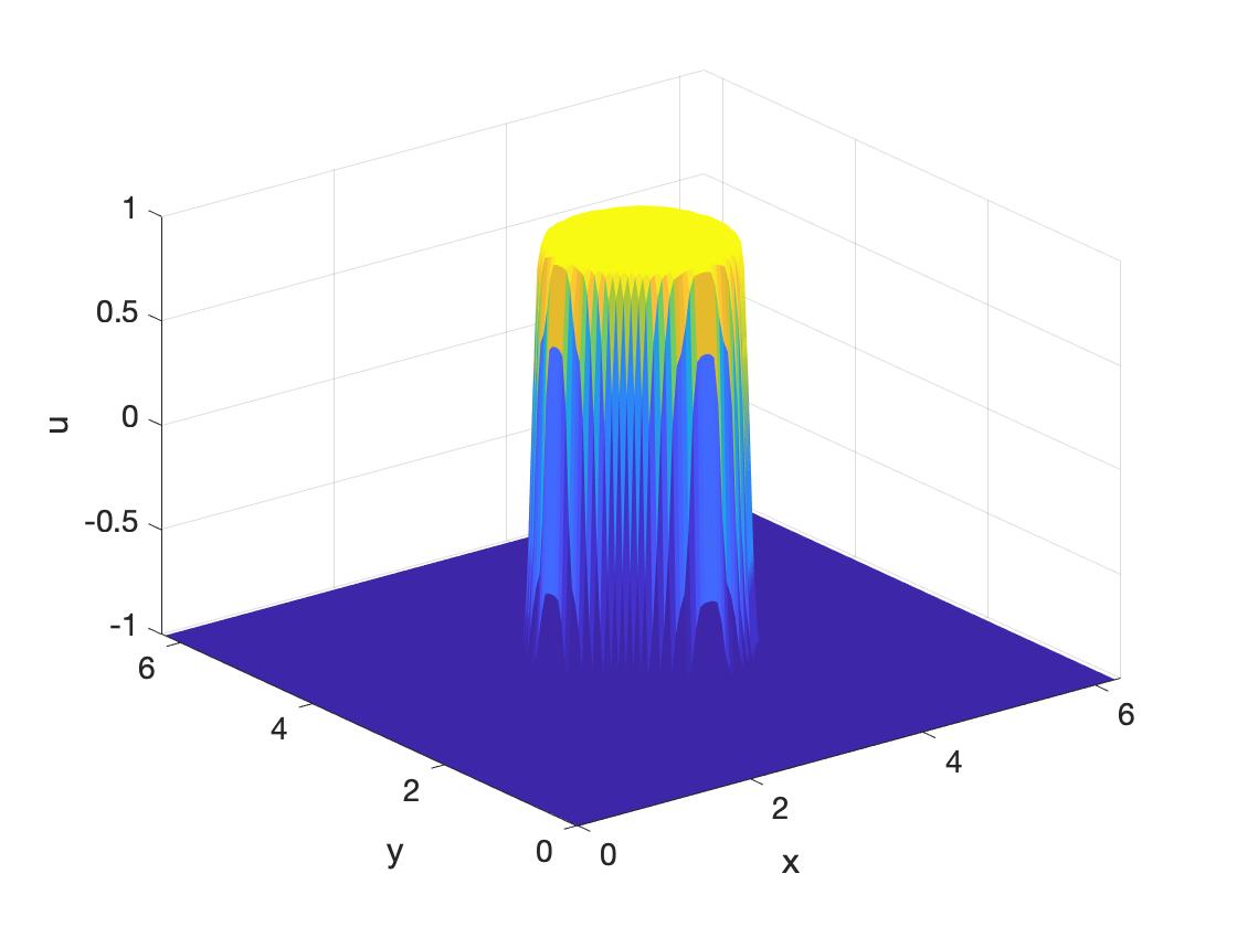
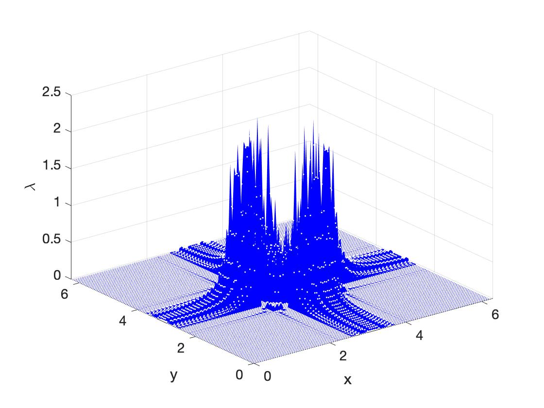
Figure 1: Numerical solution $u$ and Lagrange multiplier $\lambda$ at $T=0.001$ computed by scheme (2.8)-(2.9) with $k=2$ and $\delta t=10^{-6}$.

6.1.2 Comparison with a usual semi-implicit scheme

We consider the Allen-Cahn equation with $\epsilon^{2}=0.001$ and the initial condition

(6.101) $$\begin{split}u(x,y,0)&=\tanh(\frac{1-\sqrt{(x-\pi)^{2}+(y-3\pi/2)^{2}}}{\sqrt{2}\epsilon})\\ &+\tanh(\frac{1-\sqrt{(x-\pi)^{2}+(y-3\pi/4)^{2}}}{\sqrt{2}\epsilon})+1.\end{split}$$

We use the scheme (5.86)-(5.87) and its usual semi-implicit version:

(6.102) $$\begin{split}&\frac{u^{n+1}-u^{n}}{\delta t}+\mathcal{L}(\frac{3}{4}u^{n+1}+\frac{1}{4}u^{n-1})+\mathcal{N}(\frac{3}{2}u^{n}-\frac{1}{2}u^{n-1})=0,\end{split}$$

with time step $\delta t=8\times 10^{-4}$ and $128^{2}$ Fourier modes.

In Figure. 2, we plot the numerical solution $u$ at $T=0.08$ and $T=0.4$ using the semi-implicit scheme (6.102) and the bound-preserving scheme (5.86)-(5.87). It is observed that the numerical solution by the bound-preserving scheme stays within $[-1,1]$, while that by the semi-implicit scheme (6.102) violates this property. The Lagrange multiplier $\lambda$ by the bound-preserving scheme (5.86)-(5.87) are also shown in Figure. 2. In Fig. 3, we plot the evolution of $\max\{u\}$ and $\min\{u\}$ by both schemes.

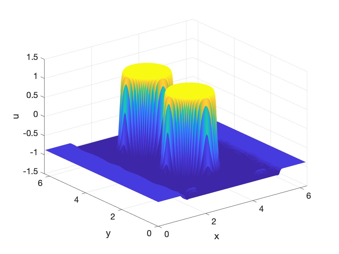
(a) $u$ at $T=0.08$ by (6.102).

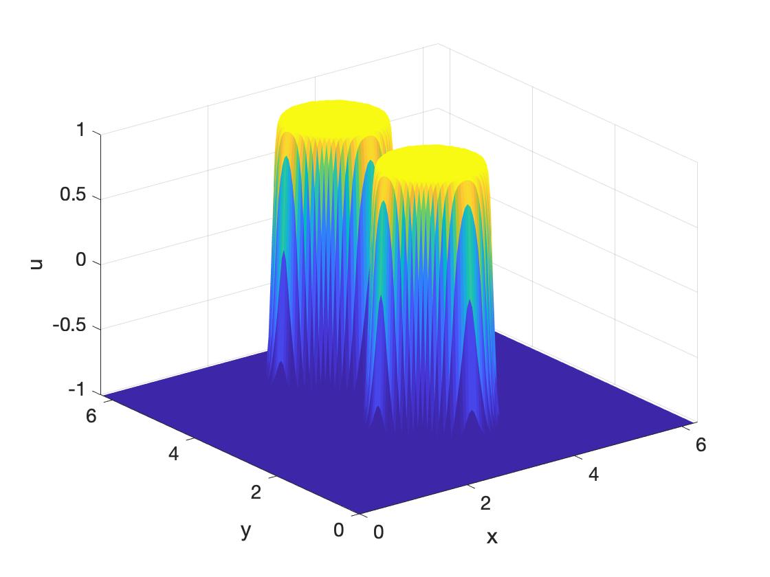
(b) $u$ at $T=0.08$ by (5.86)-(5.87).

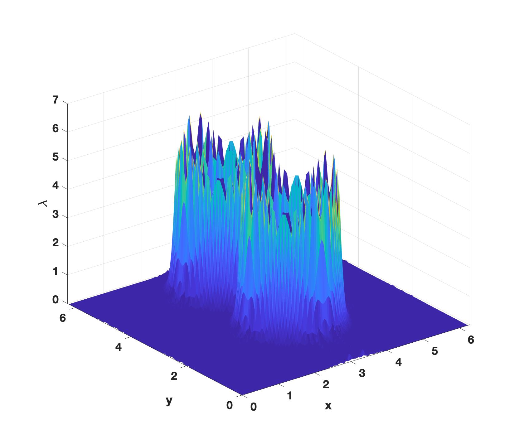
(c) $\lambda$ at $T=0.08$.

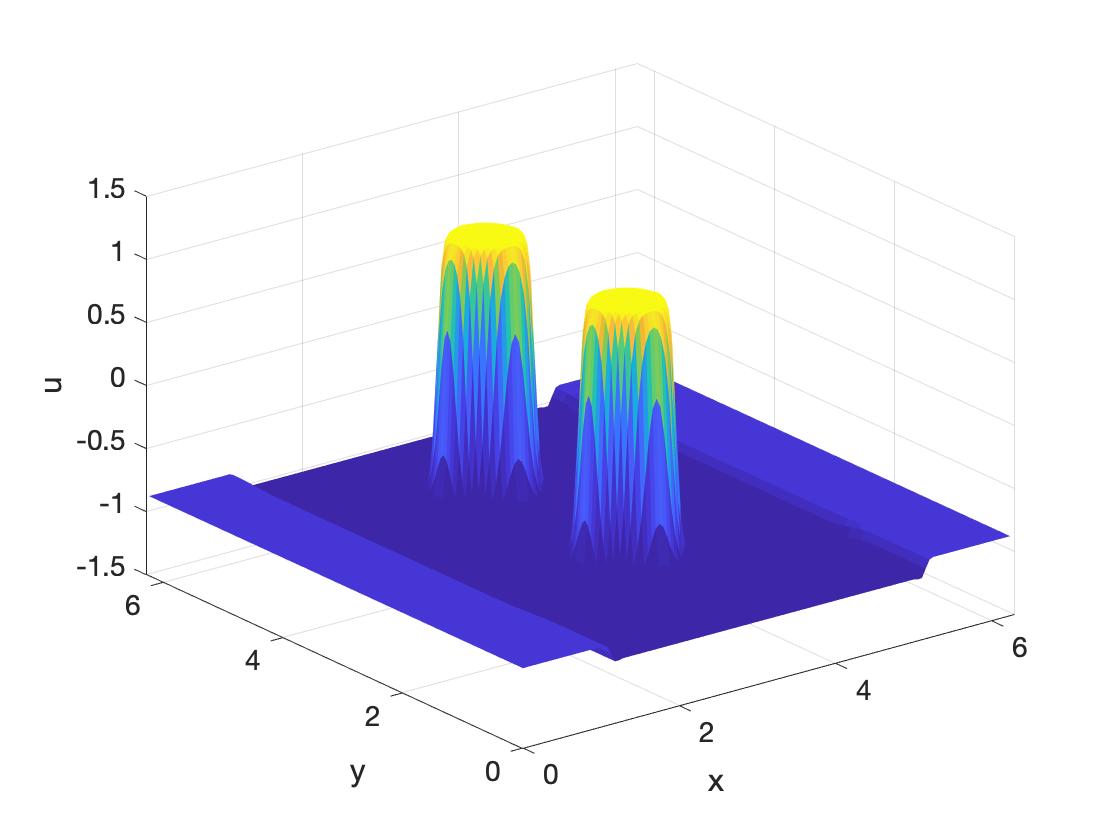
(d) $u$ at $T=0.4$ by (6.102).

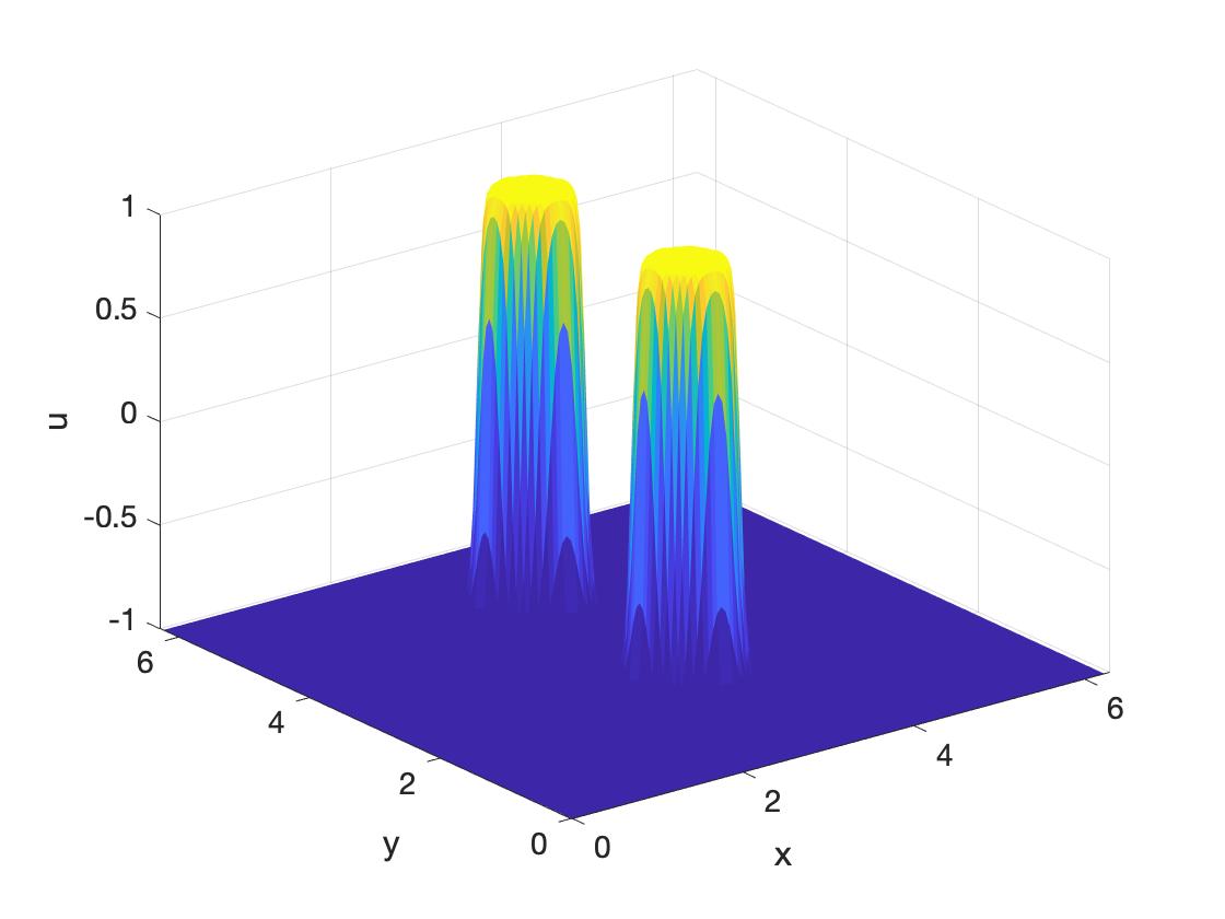
(e) $u$ at $T=0.4$ (5.86)-(5.87).

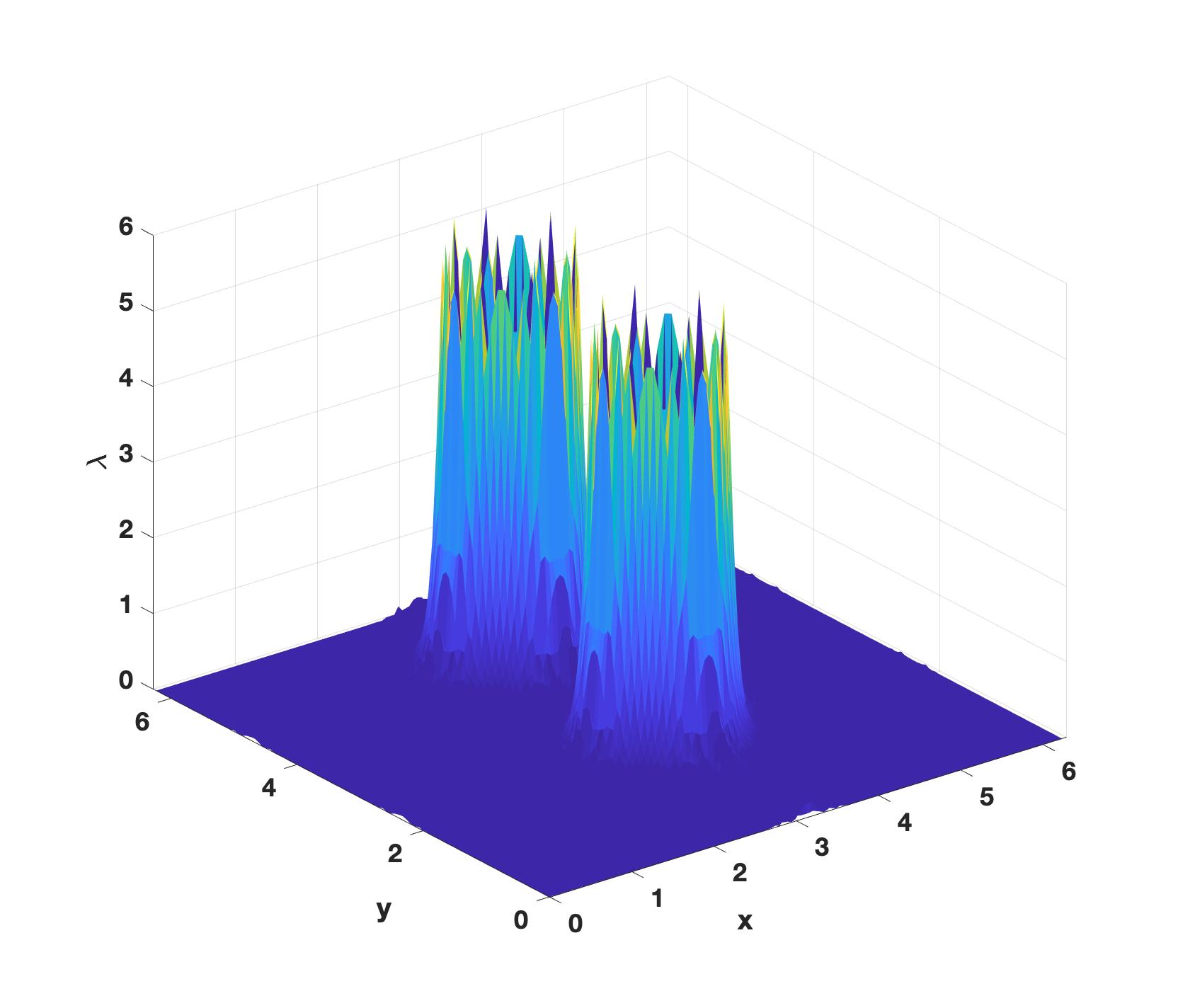
(f) $\lambda$ at $T=0.4$.

Figure 2: (a)-(d): Numerical solutions at $T=0.08,0.4$ computed by (6.102). (b)-(c) and (e)-(f): numerical solutions and Lagrange multiplier $\lambda$ at $T=0.08,0.4$ computed by (5.86)-(5.87).

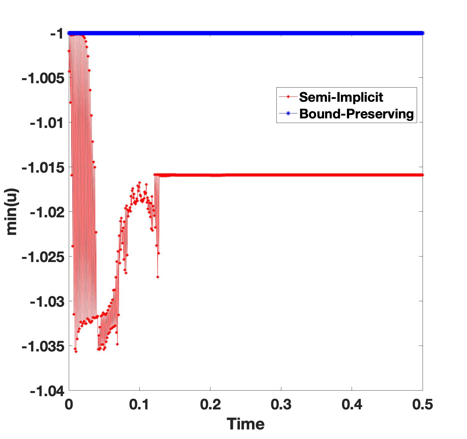
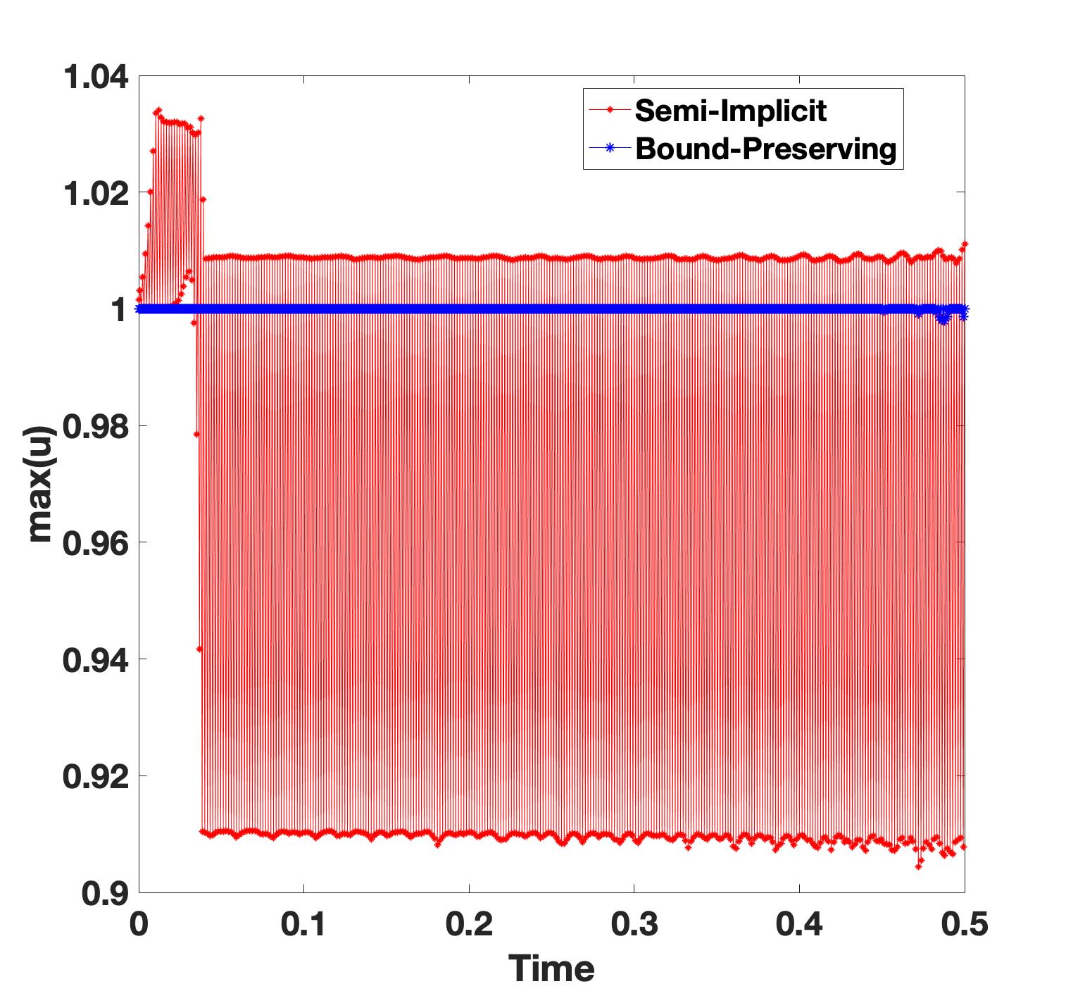
Figure 3: Evolution of $\max\{u\}$ and $\min\{u\}$ with respect to time for the semi-implicit scheme (6.102) and the bound-preserving scheme (5.86)-(5.87).

6.2 Cahn-Hilliard equation

We now consider the Cahn-Hilliard equation (5.88) with the initial condition

(6.103) $$u_{0}(x,y)=0.2+0.05\,{\rm rand}(x,y),$$

where function ${\rm rand}(x,y)$ is a uniformed distributed random function with values in $(-1,1)$. We set $\theta_{0}=5$ and $\epsilon=0.1$, and use $\delta t=10^{-5}$ with $128^{2}$ Fourier modes in $(0,2\pi)^{2}$. We first use the following semi-implicit scheme

(6.104) $$\begin{split}&\frac{3{u}^{n+1}-4u^{n}+u^{n-1}}{2\delta t}=\nabla\cdot(M(2u^{n}-u^{n-1})\nabla\mu^{n+1}),\\ &\mu^{n+1}=-\epsilon^{2}\Delta u^{n+1}+{\rm ln}(1+2u^{n}-u^{n-1})-{\rm ln}(1-2u^{n}+u^{n-1})-\theta_{0}(2u^{n}-u^{n-1}),\end{split}$$

and found that it blows up at $t\approx.025$ when $\|u^{n}\|_{l^{\infty}}>1$ due to the singular potential. We then use the bound preserving scheme (5.91)-(5.92) with $\delta=0.01$ to compute up to $t=0.1$, and plot in Fig. 4 the evolution of $\max_{\boldsymbol{z}\in\Sigma_{N}}u^{n}(\boldsymbol{z})$ and $\min_{\boldsymbol{z}\in\Sigma_{N}}u^{n+1}(\boldsymbol{z})$ by the scheme (6.104) up to $t\approx.025$, and by the scheme (5.91)-(5.92) up to $t=0.1$. In Fig. 5, we plot the numerical solutions at various times which depict the coarsening process.

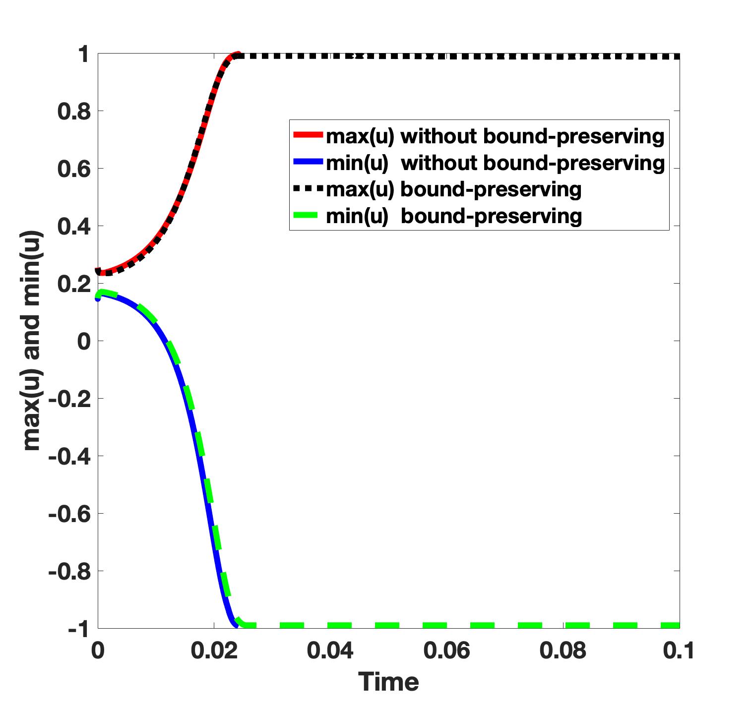
Figure 4: The evolution of $\max_{i,j}{u^{n}_{i,j}}$ and $\min_{i,j}{u^{n}_{i,j}}$ with respect to time computed by the scheme (6.104) up to $t\approx.025$, and by the scheme (5.91)-(5.92) up to $t=0.1$.

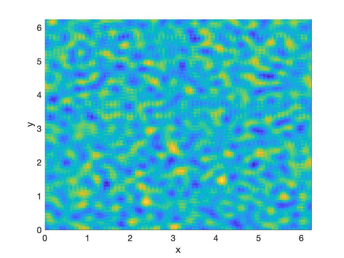
(a) $t=0.001$

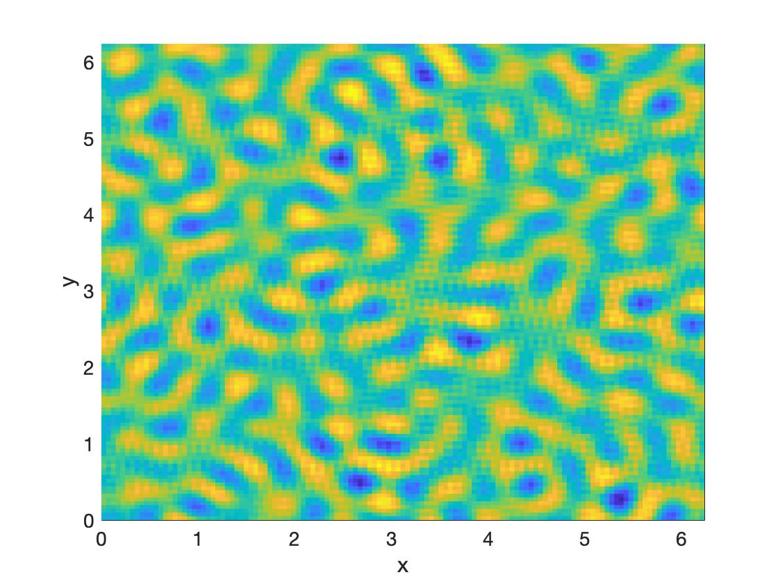
(b) $t=0.02$

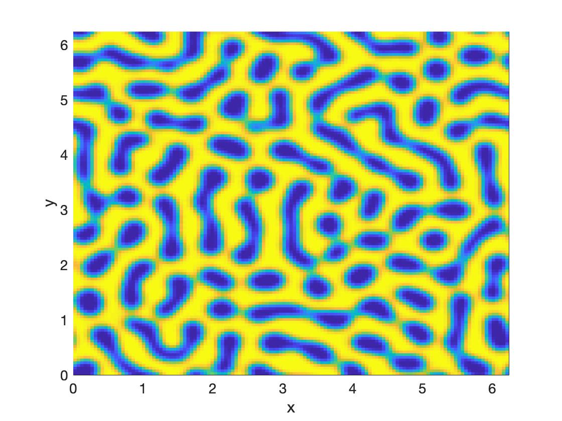
(c) $t=0.05$

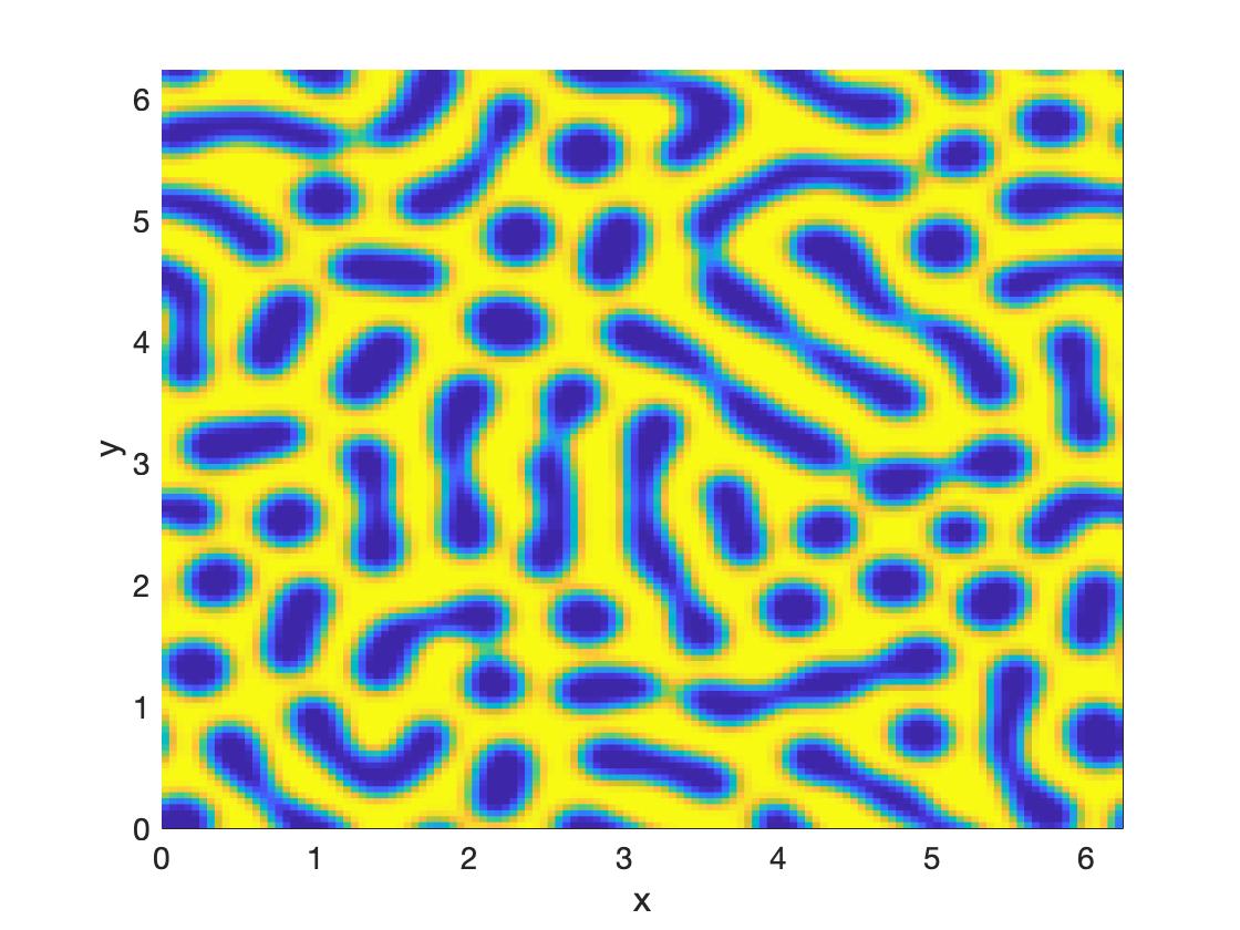
(d) $t=0.1$

Figure 5: Numerical solutions of Cahn-Hilliard equation at $t=0.001,0.02,0.05,0.1$ computed by the scheme (5.91)-(5.92).

6.3 Fokker-Planck equation

As the final example, we consider the Fokker-Planck equation (5.93) with periodic boundary condition whose solution remains in $[0,1]$ and is mass preserving. We present below simulations of (5.93) on the domain $(-2\pi,2\pi)$ with the initial condition $u(x,0)=-e^{-\frac{(x-1)^{2}}{0.4}}$ using three second-order schemes: a usual semi-implicit scheme

(6.105) $$\begin{split}&\frac{3u^{n+1}-4u^{n}+u^{n-1}}{2\delta t}=\partial_{x}(x(2u^{n}-u^{n-1})(1-2u^{n}+u^{n-1})+\partial_{x}u^{n+1}),\end{split}$$

the bound-preserving scheme (5.96)-(5.97) and the mass conservative, bound-preserving scheme (5.98)-(5.99).

In Fig. 6, we plot the numerical results using the semi-implicit scheme (6.105) and the bound-preserving scheme (5.96)-(5.97) with 32 Fourier modes and $\delta t=10^{-4}$. We observe that while the two numerical solutions look very similar, the minimum value by the semi-implicit scheme (6.105) does become negative in a short period at the beginning, while the numerical solutions by (5.96)-(5.97) remain in $[0,1]$.

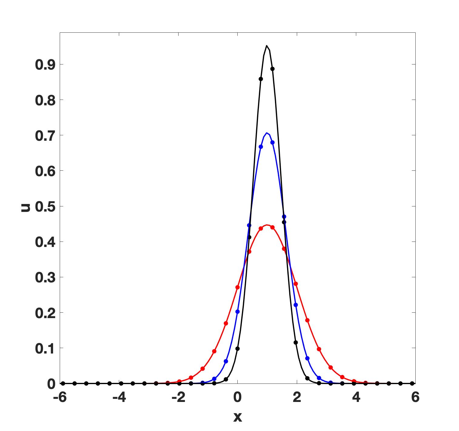
(a) By the bound-preserving scheme.

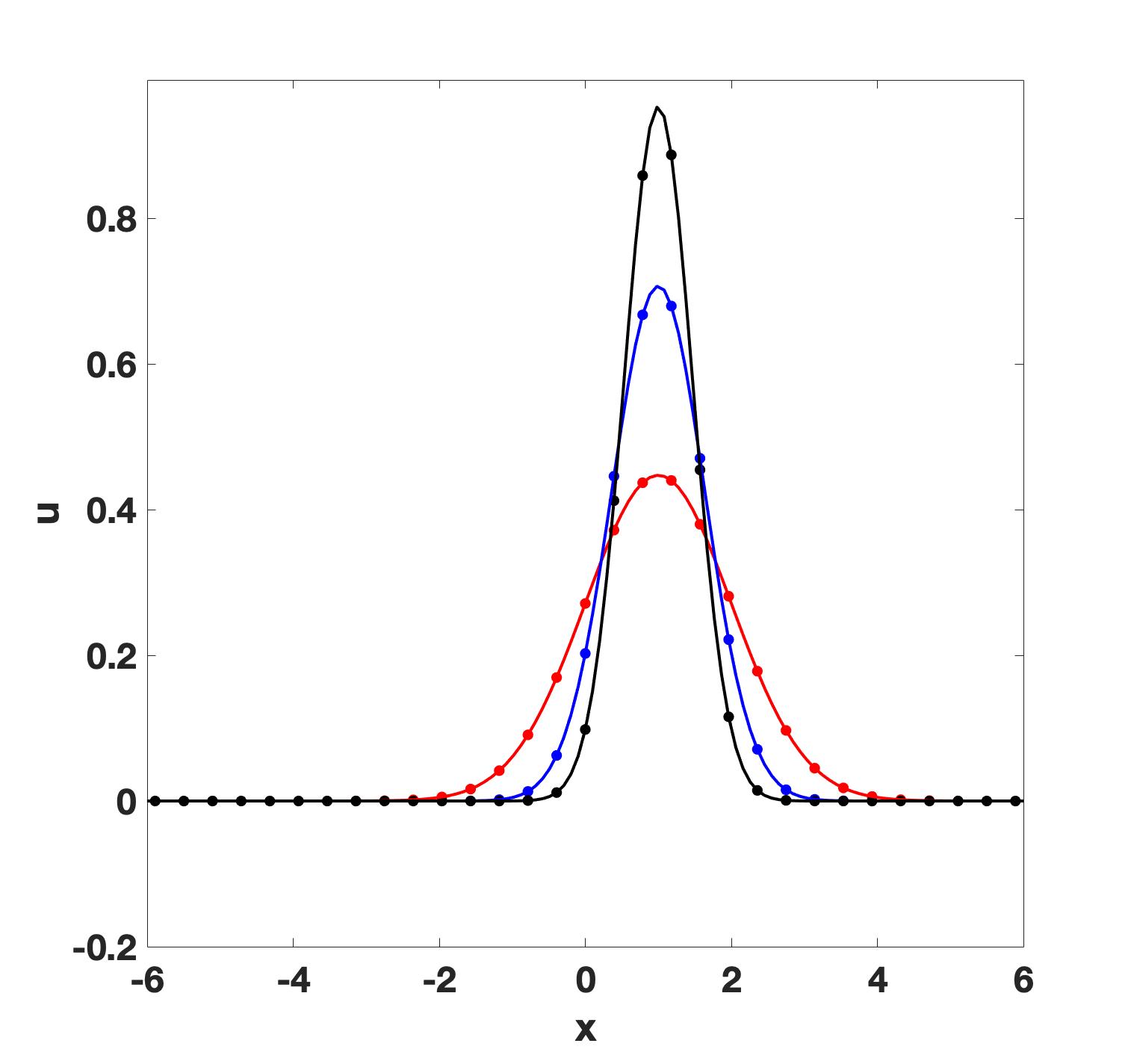
(b) By the semi-implicit scheme.

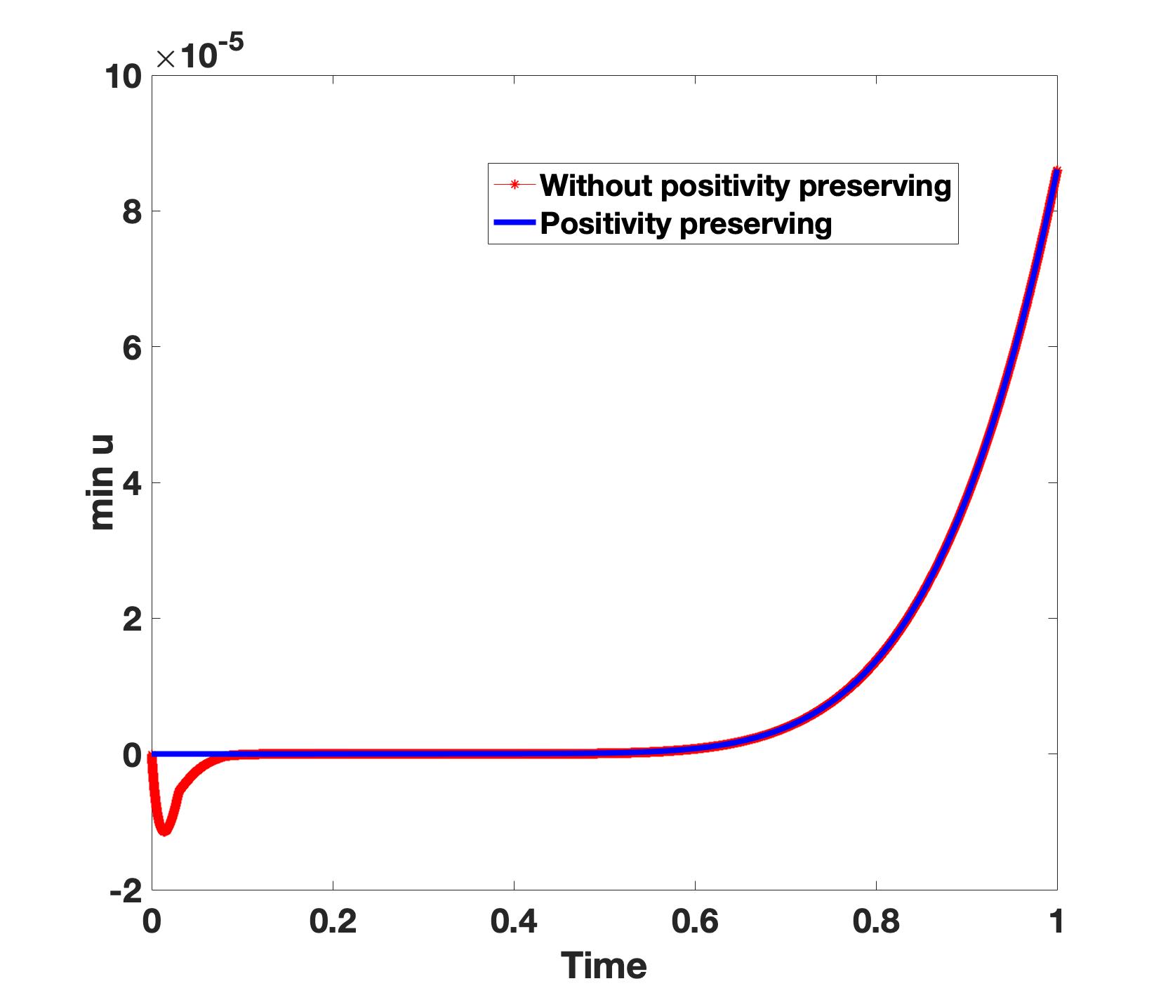
(c) Evolutions of minimum values

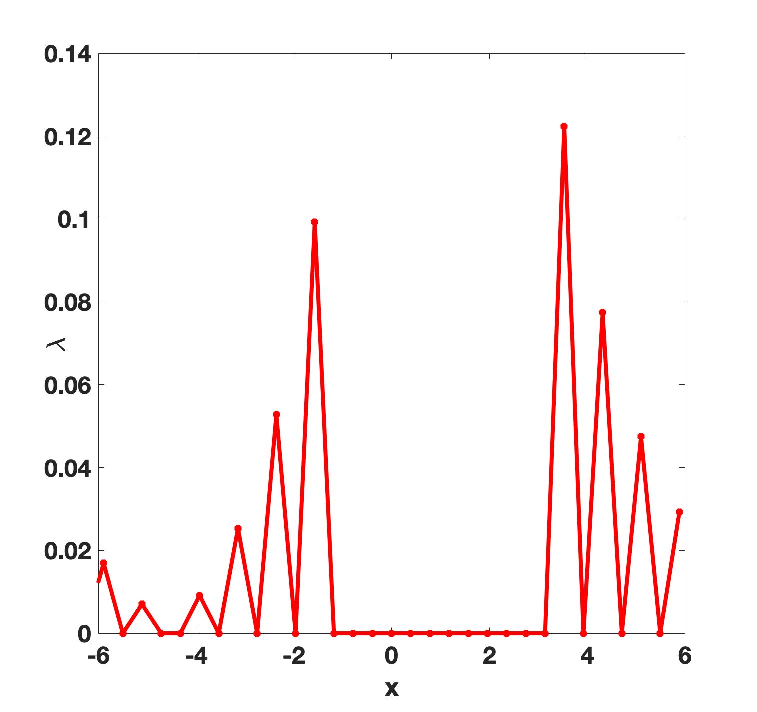
(d) $\lambda$ at $t=0.01$

Figure 6: (a)-(b) :Numerical solutions computed with $32$ Fourier modes plotted on the $256$ uniform grids using (5.96)-(5.97) and -(6.105). (c): Evolutions of minimal values using (5.96)-(5.97) and -(6.105). (d): Lagrange multiplier $lambda$ at $t=0.01$ using (5.96)-(5.97).

In Fig. 7, we plot the numerical results using the bound-preserving scheme (5.96)-(5.97) and the mass conservative, bound-preserving scheme (5.98)-(5.99) with 32 Fourier modes and $\delta t=10^{-4}$. We observe that (5.96)-(5.97) can not preserve mass, while (5.98)-(5.99) preserves mass exactly. Only a few iterations are needed to compute the Lagrange multiplier $\xi$ at each time step by using the mass conservative, bound-preserving scheme (5.98)-(5.99) .

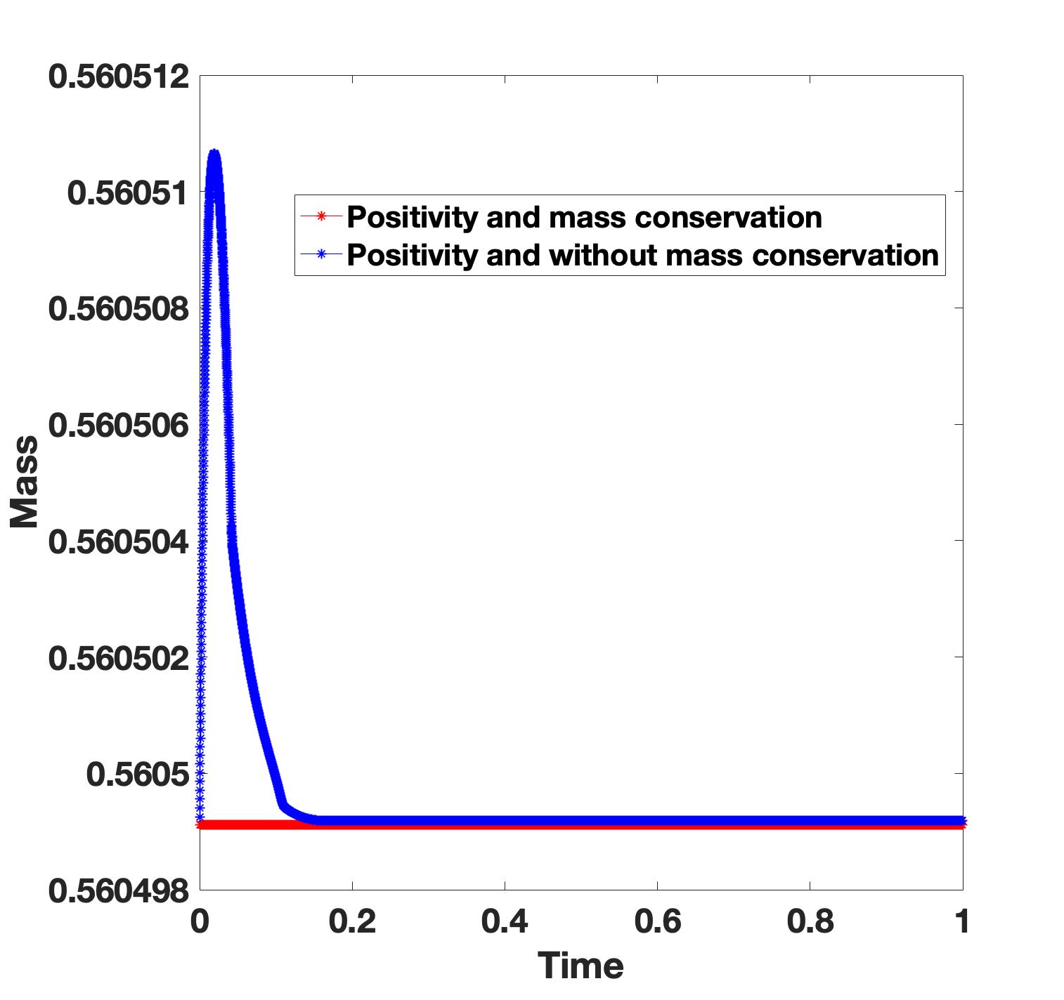
(a) Evolution of mass

(b) Solution profiles: $u$ at $t=0.01,0.1,0.4$.

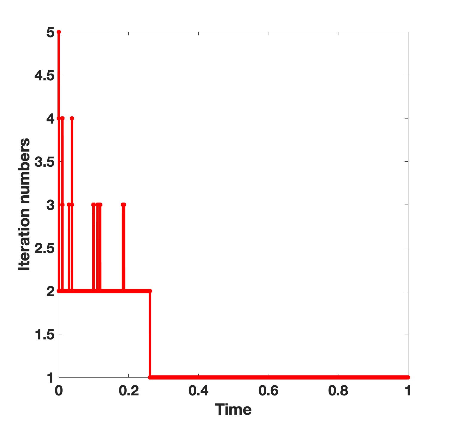
(c) Iteration number

Figure 7: (a): Evolution of mass by (5.96)-(5.97) and (5.98)-(5.99). (b): Solution profiles by (5.98)-(5.99). (c): Iteration numbers for solving $\xi^{n+1}$ at each time step of (5.98)-(5.99).

7 Concluding remarks

We constructed efficient and accurate bound and/or mass preserving schemes for a class of semi-linear and quasi-linear parabolic equations using the Lagrange multiplier approach.

First, we constructed a class of multistep IMEX schemes (2.8)-(2.9) for the semi-discrete problem (2.4) with a Lagrange multiplier to enforce bound preserving, which is an approximation to the original PDE (1.1). Hence, the scheme (2.8)- (2.9) is a $k$-th order approximation in time for both (2.4) and (1.1). In particular, the (2.8)-(2.9) can be very useful if one is interested in the discrete problem (2.4) without a background PDE.

Then, we pointed out in Remark 2.1 that by dropping out the term $B_{k-1}(\lambda_{h}^{n}g^{\prime}(u_{h}^{n}))$ in (2.8) and (2.9), we recover the usual cut-off scheme which is a $k$-th order approximation in time for (1.1), but only a first-order approximation in time for (2.4). Thus, our presentation provided an alternative interpretation of the cur-off approach, and moreover, allowed us to construct new cut-off implicit-explicit (IMEX) schemes with mass conservation.

We also established some stability results involving norms with derivatives under a general setting, and derived optimal error estimates for a second-order bound preserving scheme with a hybrid spectral discretization in space.

Finally, we applied our approach to several typical PDEs which preserve bound and/or mass, and presented ample numerical results to validate our approach. The approach presented in this paper is quite general and can be used to develop bound preserving schemes for other bound preserving PDEs such as the Keller-Segel equations [18].

References

- [1] Samuel M Allen and John W Cahn. A microscopic theory for antiphase boundary motion and its application to antiphase domain coarsening. Acta metallurgica, 27(6):1085–1095, 1979.
- [2] Maïtine Bergounioux, Kazufumi Ito, and Karl Kunisch. Primal-dual strategy for constrained optimal control problems. SIAM Journal on Control and Optimization, 37(4):1176–1194, 1999.
- [3] John W Cahn and John E Hilliard. Free energy of a nonuniform system. i. interfacial free energy. The Journal of chemical physics, 28(2):258–267, 1958.
- [4] Claudio Canuto, M Yousuff Hussaini, Alfio Quarteroni, A Thomas Jr, et al. Spectral methods in fluid dynamics. Springer Science & Business Media, 2012.
- [5] José A Carrillo, Jesús Rosado, and Francesco Salvarani. 1d nonlinear Fokker–Planck equations for fermions and bosons. Applied Mathematics Letters, 21(2):148–154, 2008.
- [6] Qing Cheng and Jie Shen. A new Lagrange multiplier approach for constructing structure preserving schemes, i. positivity preserving. arXiv preprint arXiv:2107.00504, 2021.
- [7] Philippe G Ciarlet. Discrete maximum principle for finite-difference operators. Aequationes mathematicae, 4(1-2):266–268, 1970.
- [8] Philippe G Ciarlet and P-A Raviart. Maximum principle and uniform convergence for the finite element method. Computer Methods in Applied Mechanics and Engineering, 2(1):17–31, 1973.
- [9] Arnaud Debussche and Lucia Dettori. On the Cahn-Hilliard equation with a logarithmic free energy. Nonlinear Analysis: Theory, Methods & Applications, 24(10):1491–1514, 1995.
- [10] Jérôme Droniou and Christophe Le Potier. Construction and convergence study of schemes preserving the elliptic local maximum principle. SIAM Journal on numerical analysis, 49(2):459–490, 2011.
- [11] Qiang Du, Lili Ju, Xiao Li, and Zhonghua Qiao. Maximum principle preserving exponential time differencing schemes for the nonlocal Allen–Cahn equation. SIAM Journal on numerical analysis, 57(2):875–898, 2019.
- [12] Qiang Du, Lili Ju, Xiao Li, and Zhonghua Qiao. Maximum bound principles for a class of semilinear parabolic equations and exponential time-differencing schemes. SIAM Review., 63(2):317–359, 2021.
- [13] Charles M Elliott and Harald Garcke. On the Cahn–Hilliard equation with degenerate mobility. SIAM Journal on mathematical analysis, 27(2):404–423, 1996.
- [14] Francisco Facchinei and Jong-Shi Pang. Finite-dimensional variational inequalities and complementarity problems. Springer Science & Business Media, 2007.
- [15] Sigal Gottlieb and Cheng Wang. Stability and convergence analysis of fully discrete fourier collocation spectral method for 3-d viscous burgers’ equation. Journal of Scientific Computing, 53(1):102–128, 2012.
- [16] Patrick T Harker and Jong-Shi Pang. Finite-dimensional variational inequality and nonlinear complementarity problems: a survey of theory, algorithms and applications. Mathematical programming, 48(1):161–220, 1990.
- [17] Kazufumi Ito and Karl Kunisch. Lagrange multiplier approach to variational problems and applications. SIAM, 2008.
- [18] Evelyn F. Keller and Lee A. Segel. Initiation of slime mold aggregation viewed as an instability. Journal of Theoretical Biology, 26(3):399 – 415, 1970.
- [19] Maojun Li, Yongping Cheng, Jie Shen, and Xiangxiong Zhang. A bound-preserving high order scheme for variable density incompressible Navier-Stokes equations. Journal of Computational Physics, 425:109906, 2021.
- [20] Hong-lin Liao, Tao Tang, and Tao Zhou. A second-order and nonuniform time-stepping maximum-principle preserving scheme for time-fractional Allen-Cahn equations. Journal of Computational Physics, 414:109473, 2020.
- [21] Hailiang Liu and Hui Yu. Maximum-principle-satisfying third order discontinuous galerkin schemes for Fokker–Planck equations. SIAM Journal on Scientific Computing, 36(5):A2296–A2325, 2014.
- [22] Changna Lu, Weizhang Huang, and Erik S. Van Vleck. The cutoff method for the numerical computation of nonnegative solutions of parabolic PDEs with application to anisotropic diffusion and lubrication-type equations. Journal of Computational Physics, 242:24–36, 2013.
- [23] Hannes Risken. Fokker-planck equation. In The Fokker-Planck Equation, pages 63–95. Springer, 1996.
- [24] Jie Shen, Tao Tang, and Li-Lian Wang. Spectral methods: algorithms, analysis and applications, volume 41. Springer Science & Business Media, 2011.
- [25] Zheng Sun, José A Carrillo, and Chi-Wang Shu. A discontinuous galerkin method for nonlinear parabolic equations and gradient flow problems with interaction potentials. Journal of Computational Physics, 352:76–104, 2018.
- [26] Jaap JW van der Vegt, Yinhua Xia, and Yan Xu. Positivity preserving limiters for time-implicit higher order accurate discontinuous galerkin discretizations. SIAM Journal on scientific computing, 41(3):A2037–A2063, 2019.
- [27] Huifang Zhou, Zhiqiang Sheng, and Guangwei Yuan. Physical-bound-preserving finite volume methods for the Nagumo equation on distorted meshes. Computers & Mathematics with Applications, 77(4):1055–1070, 2019.