Improved Soft Duplicate Detection in Search-Based Motion Planning

Abstract

Search-based techniques have shown great success in motion planning problems such as robotic navigation by discretizing the state space and precomputing motion primitives. However in domains with complex dynamic constraints, constructing motion primitives in a discretized state space is non-trivial. This requires operating in continuous space which can be challenging for search-based planners as they can get stuck in local minima regions. Previous work [1] on planning in continuous spaces introduced soft duplicate detection which requires search to compute the duplicity of a state with respect to previously seen states to avoid exploring states that are likely to be duplicates, especially in local minima regions. They propose a simple metric utilizing the euclidean distance between states, and proximity to obstacles to compute the duplicity. In this paper, we improve upon this metric by introducing a kinodynamically informed metric, subtree overlap, between two states as the similarity between their successors that can be reached within a fixed time horizon using kinodynamic motion primitives. This captures the intuition that, due to robot dynamics, duplicate states can be far in euclidean distance and result in very similar successor states, while non-duplicate states can be close and result in widely different successors. Our approach computes the new metric offline for a given robot dynamics, and stores the subtree overlap value for all possible relative state configurations. During search, the planner uses these precomputed values to speed up duplicity computation, and achieves fast planning times in continuous spaces in addition to completeness and sub-optimality guarantees. Empirically, we show that our improved metric for soft duplicity detection in search-based planning outperforms previous approaches in terms of planning time, by a factor of $1.5$ to $2$$\times$ on $3$D and $5$D planning domains with highly constrained dynamics.

I Introduction and Related Work

Planning motion for robots such as manipulators [2], unmanned aerial vehicles [3] and humanoids [4] with complex kinodynamic constraints is challenging as it requires us to compute trajectories that are both collision-free and feasible to execute on the robot. The traditional approach to kinodynamic planning using search-based planners is to discretize the continuous state space into cells, and the search traverses only through the centers of the cells [5]. To account for the kinodynamic nature of the planning problem, these approaches [6, 7] make use of motion primitives which are precomputed actions that the robot can take at any state. Due to the discretization, we require that the motion primitives be able to connect from one cell center to another cell center. However, this requires solving a two-point boundary value problem [8] which may be infeasible to solve for domains with highly constrained dynamics [9]. A typical solution is to discretize the state space at a higher resolution which can blow up the size of the search space making search computationally very expensive [10].

Alternatively, we can use sampling-based approaches such as RRT [11] and RRT* [12] that have been popular in kinodynamic planning. These approaches directly plan in the continuous space by randomly sampling controls or motion primitives, and extending states [11, 13] until we reach the goal state. The major disadvantage of these approaches is that typically the solutions they generate can be quite poor in quality and lack consistency in solution (similar solutions for similar planning queries) due to randomness, unlike search-based methods. Furthermore, in motion planning domains with narrow passageways, sampling-based approaches can take a long time to find a solution as the probability of randomly sampling a state within the narrow passageway is very low [14].

Naively, one could use search-based planning directly in the continuous space. The challenge here is to ensure that the search does not unnecessarily expand similar states, which happens often when the heuristic used is not informative and does not account for the kinodynamic constraints explicitly. In such cases, the search can end up in a “local minima” region, and expand a large number of nearly identical states before exiting the region [15]. Approaches that aim to detect when the heuristic is “stagnant” [16] or avoid local minima regions in the state space [17] require either extensive domain knowledge or user input to achieve this. In order to avoid expanding similar states, approaches such as [18, 19] group states into equivalence classes that can be used for duplicate detection [20] in discrete state spaces.

A recent work [1] extends similar ideas to continuous state spaces by introducing soft duplicate detection. They define a duplicity function that assigns a value to each state during search based on how likely that state can contribute to the search finding a solution. The assigned duplicity is then used to penalize states that are similar to previously seen states by inflating their heuristic within a weighted A* framework [21]. Unlike past duplicate detection works, this approach does not prune away duplicate states resulting in maintaining completeness guarantees while achieving fast planning times. Their approach is shown to outperform other duplicate detection approaches such as [18, 19].

Our proposed approach builds upon this work by improving the duplicity function used, to incorporate a more kinodynamically informed notion of when a state is likely to contribute to the search finding a solution. We achieve this by using a novel metric, subtree overlap, between two states which is a similarity metric between their successors that can be reached using kinodynamic motion primitives within a fixed time horizon. We show that computing this new metric during search can be computationally very expensive and hence, we precompute the metric offline for all possible relative state configurations and store these values. During search, we use these precomputed subtree overlap values in duplicity computation to obtain $1.5$ to $2$$\times$ improvement in planning time over previous approaches, including [1], in continuous $3$D and $5$D planning domains with highly constrained dynamics. In addition to faster planning times, we also retain the completeness and sub-optimality bound guarantees of search-based methods.

II Problem Setup and Background

In this section, we will describe the problem setup and previous work on soft duplicate detection [1] as our approach builds on it. We are given a robot with state space $\mathbb{S}$ whose dynamics are constrained, and the objective is to plan a kinodynamically feasible and collision-free path from a start state $s_{\mathsf{start}}$ to any state in a goal region specified by $S_{\mathsf{goal}}\subset\mathbb{S}$. This is formulated as a search problem by constructing a lattice graph using a set of motion primitives, which are dynamically feasible actions, at any state [8]. These motion primitives define a set of successors for any state $s$ given by the set $\mathcal{S}_{1}(s)$ comprising of states that are dynamically feasible to reach from $s$. We also have a cost function $c:\mathbb{S}\times\mathbb{S}\rightarrow\mathbb{R}^{+}\cup\{0\}$ which assigns a cost $c(s,s^{\prime})$ for any motion primitive taking the robot from state $s$ to $s^{\prime}$. Finally, we assume that we are given access to an admissible heuristic function $h:\mathbb{S}\rightarrow\mathbb{R}^{+}\cup\{0\}$ which is an underestimate of the optimal path cost from any state to a goal state.

The soft duplicate detection framework, introduced in [1], requires access to a duplicity function $\mathsf{dup}:\mathbb{S}\times\mathbb{S}\rightarrow[0,1]$ which for any two states $s,s^{\prime}$ corresponds to the likelihood that they are duplicates of each other. More precisely, $\mathsf{dup}(s,s^{\prime})$ captures the (inverse) likelihood that $s$ will contribute to computing a path to $S_{\mathsf{goal}}$ given that the search has already explored $s^{\prime}$. This can be generalized (with a slight abuse of notation) to compute duplicity of a state with respect to a set of states $U$ as $\mathsf{dup}(s,U)=\max_{s^{\prime}\in U}\mathsf{dup}(s,s^{\prime})$. This framework is used within Weighted A* [21] search by using a state-dependent heuristic inflation factor given by, $\epsilon(s)=\max(\epsilon_{\mathsf{max}}\cdot\mathsf{dup}(s,U),\epsilon_{0})$ where $\epsilon_{0}$ and $\epsilon_{\mathsf{max}}$ are constants such that $\epsilon_{\mathsf{max}}>\epsilon_{0}>1$. The set $U$ consists of the states in the priority queues $\mathsf{OPEN}$ (containing states that the search may expand,) and $\mathsf{CLOSED}$ (containing states that search has already expanded,) i.e. $U=\mathsf{OPEN}\cup\mathsf{CLOSED}$. For completeness, we present Weighted A* with soft duplicate detection using $\mathsf{dup}(s,U)$ from [1] in Algorithm 1. Note that states with higher duplicity have a higher inflation factor leading to giving them lower priority in $\mathsf{OPEN}$ maintained by weighted A*, and vice versa.

Algorithm 1 Weighted A* with Soft Duplicate Detection [1]

1:Input: Duplicity Function $\mathsf{dup}$, constants $\epsilon_{0},\epsilon_{\mathsf{max}}$

2:Set $g(s_{\mathsf{start}})=0$ $\triangleright$ $g$-value for other states set to $\infty$

3:Set $\mathsf{CLOSED}=\phi$, and $\mathsf{OPEN}=\{s_{\mathsf{start}}\}$

4:while $s_{\mathsf{goal}}\notin\mathsf{CLOSED}$ and $\mathsf{OPEN}\neq\phi$ do

5:    Set $U=\mathsf{OPEN}\cup\mathsf{CLOSED}$

6:    Pop $s$ with the smallest $f$-value from $\mathsf{OPEN}$

7:    $\mathsf{CLOSED}=\mathsf{CLOSED}\cup\{s\}$

8:    for $s^{\prime}\in\mathcal{S}_{1}(s)$ do

9:         if $s^{\prime}\notin U$ then

10:             $\epsilon(s^{\prime})=\max(\epsilon_{\mathsf{max}}\cdot\mathsf{dup}(s^{\prime},U),\epsilon_{0})$          

11:         if $g(s^{\prime})>g(s)+c(s,s^{\prime})$ then

12:             $g(s^{\prime})=g(s)+c(s,s^{\prime})$

13:             $f(s^{\prime})=g(s^{\prime})+\epsilon(s^{\prime})\cdot h(s^{\prime})$

14:             $\mathsf{OPEN}=\mathsf{OPEN}\cup\{s^{\prime}\}$ $\triangleright$ Key is $f$-value              

15:if $s_{\mathsf{goal}}\in\mathsf{CLOSED}$ then

16:    return Path found from $s_{\mathsf{start}}$ to $s_{\mathsf{goal}}$

17:return No path found

Wei et. al. [1] propose using a duplicity function $\mathsf{dup}_{\mathcal{E}}$ that is defined as follows,

$$\mathsf{dup}_{\mathcal{E}}(s,U)=1-\frac{d_{\mathsf{NN}}(s,U)}{R\cdot\gamma(s_{\mathsf{parent}})}$$ (1)

where $d_{\mathsf{NN}}(s,U)=\min_{s^{\prime}\in U}\mathsf{dist}(s,s^{\prime})$, $\mathsf{dist}$ is a euclidean distance metric defined on $\mathbb{S}$, $R$ is a distance normalization constant, and $\gamma(s_{\mathsf{parent}})$ is the valid successor ratio that computes the proportion of successor states of the parent of $s$ that are not in collision with obstacles. Specifically, for any state $s$ we have

$$\gamma(s)=\frac{\text{\# collision-free states in $\mathcal{S}_{1}(s)$ }}{\text{\# states in $\mathcal{S}_{1}(s)$}}$$ (2)

Intuitively, the duplicity function in equation (1) assigns higher duplicity to states that are close to each other, and vice versa. It also assigns lower duplicity for states that are in the vicinity of obstacles to ensure that the search does not penalize states within tight workspaces such as narrow passageways.

III Approach

In this section, we will present our novel metric for duplicity computation in the soft duplicate detection framework. We will start with introducing subtree overlap, a metric that accounts for kinodynamic constraints explicitly. Subsequently, we present simple examples to motivate why we can expect subtree overlap to be a better indication of duplicity when compared to using euclidean distance alone. Finally, we present our approach where we precompute subtree overlap values, given robot dynamics, for all possible relative state configurations, and use the stored precomputed values during search to speed up planning.

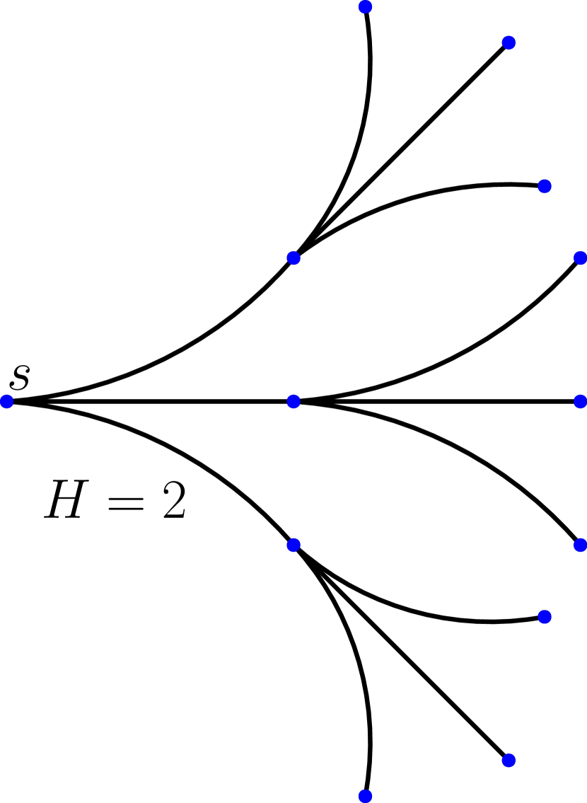
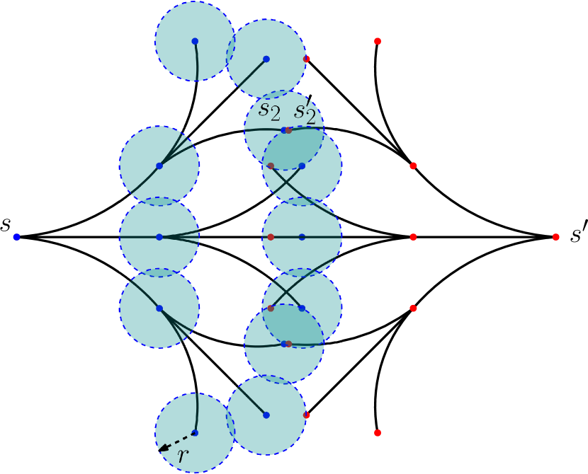
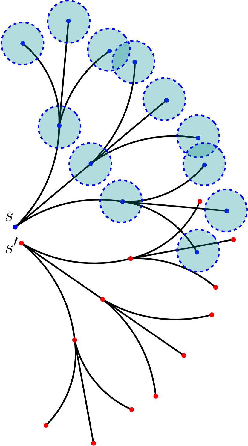
Figure 1: (left) Example subtree $\mathcal{S}_{2}(s)$ constructed at a state $s$ with a depth $H=2$. (middle) Two states $s,s^{\prime}$ that are far from each other but have significant overlap in subtrees resulting in $\eta_{2}(s,s^{\prime})=\frac{7}{12}$. The circles have a radius $r$ and are centered on each state in $\mathcal{S}_{2}(s)$. (right) Two states $s,s^{\prime}$ that are close to each other but have no overlap in subtrees resulting in $\eta_{2}(s,s^{\prime})=0$

III-A Subtree Overlap

Given a set of states $U$ that have already been encountered by the search, a new state $s$ is useful if it helps the search explore a new region of the state space that would not have been explored by expanding states in $U$. This observation allows us to come up with a kinodynamically informed metric for duplicate detection. Let $\mathcal{S}_{H}(s)$ denote the successors of state $s$ that are dynamically feasible to reach through the execution of $H$ (or less) motion primitives in sequence. This set can be represented using a subtree, as shown in Figure 1(left), rooted at $s$ and with a depth $H$. Observe that this subtree captures the region of state space that will be potentially explored within $H$ motion primitives when we expand the state $s$ during search.

For a new state $s$ which is being added to $\mathsf{OPEN}$ whose duplicity needs to be evaluated (see Algorithm 1,) we first construct the subtree $\mathcal{S}_{H}(s)$ for some fixed $H>0$. To understand if expanding $s$ allows us to explore a new region of the state space, we can consider any state $s^{\prime}\in U=\mathsf{OPEN}\cup\mathsf{CLOSED}$ and construct the subtree $\mathcal{S}_{H}(s^{\prime})$ that contains the region of state space that can be explored by expanding $s^{\prime}$. Comparing $\mathcal{S}_{H}(s^{\prime})$ with $\mathcal{S}_{H}(s)$ allows us to evaluate the relative utility of $s$ in computing a path to a goal in $S_{\mathsf{goal}}$ given that the search has already seen state $s^{\prime}$. To capture this quantity precisely, we define the metric subtree overlap of a state $s$ with another state $s^{\prime}$ denoted by $\eta_{H}(s,s^{\prime})$.

The subtree overlap $\eta_{H}(s,s^{\prime})$ is computed as the proportion of states in subtree $\mathcal{S}_{H}(s)$ that “overlap” with any state in the subtree $\mathcal{S}_{H}(s^{\prime})$. We consider two states to be overlapping if the euclidean distance between them is less than a small constant $r$, and they lie along the same depth in their respective subtrees. For example, consider state $s_{2}$ that is at depth $2$ in the subtree $\mathcal{S}_{H}(s)$ as shown in Figure 1(middle). If the subtree $\mathcal{S}_{H}(s^{\prime})$ contains a state $s^{\prime}_{2}$ that is also at depth $2$ and is less than $r$ distance away from $s_{2}$, then we consider $s_{2}$ to be overlapping with $s^{\prime}_{2}$. Thus we have,

$$\eta_{H}(s,s^{\prime})=\frac{\text{\# states in $\mathcal{S}_{H}(s)$ that overlap with $\mathcal{S}_{H}(s^{\prime})$}}{\text{\# states in $\mathcal{S}_{{H}}(s)$}}$$ (3)

Intuitively, when we have a high $\eta_{H}(s,s^{\prime})$ (close to $1$) then the state $s$ is likely to be a duplicate of $s^{\prime}$ as they lead to very similar successors. One such example is shown in Figure 1 (middle) where we have two states $s,s^{\prime}$ that are far in euclidean distance but result in similar successors and thus, have a high $\eta_{H}(s,s^{\prime})$. Using euclidean distance alone would lead us to incorrectly conclude that $s,s^{\prime}$ are not duplicates.

On the other hand, if we have a low $\eta_{H}(s,s^{\prime})$ (close to $0$) then both states lead to widely different successors, hence are not likely to be duplicates of each other. An example of this is shown in Figure 1 (right) where we have two states $s,s^{\prime}$ that are close to each other, but have minimal overlap in successors and thus, have a low $\eta_{H}(s,s^{\prime})$. These states would be incorrectly considered duplicates if we solely used euclidean distance.

III-B Duplicate Detection using Subtree Overlap

In this section, we will describe how we use the subtree overlap metric presented in Section III-A to compute the duplicity. Given a decision boundary parameter $c\in[0,1]$ and a distance normalization constant $R>>r$ (similar to equation (1)) we have,

$$\mathsf{dup}_{\mathcal{S}}(s,s^{\prime})=1-\frac{d(s,s^{\prime})(1+c-\eta_{H}(s,s^{\prime}))}{R\cdot\gamma(s_{\mathsf{parent}})}$$ (4)

where $d(s,s^{\prime})$ is the euclidean distance between $s$ and $s^{\prime}$, and $\gamma$ is the valid successor ratio as defined in equation (2). We chose $R$ such that $\mathsf{dup}_{\mathcal{S}}(s,s^{\prime})\in[0,1]$.

To use the proposed duplicity function $\mathsf{dup}_{\mathcal{S}}$ in the framework of Algorithm 1 we need to define how we compute $\mathsf{dup}_{\mathcal{S}}(s,U)$ for a set of states $U$. If we naively construct the subtree for all states $s^{\prime}$ in $U=\mathsf{OPEN}\cup\mathsf{CLOSED}$, it can be very expensive computationally as constructing the subtree involves expanding several states and querying all of their successors. However, computing subtree overlap, with a fixed depth $H$, between states that are very far from each other can be unnecessary as they would most likely not have any overlap in successors. Thus, to reduce our computation budget, we only compute the subtree overlap with states in $U$ that are within a euclidean distance of $R$. We obtain the set of states $U_{R}$ that are within a distance of $R$ by maintaining all states in $U$ in a kd-tree [22]. A similar trick was also used in [1]. Thus we have,

$$\mathsf{dup}_{\mathcal{S}}(s,U)=\max_{s^{\prime}\in U_{R}}\mathsf{dup}_{\mathcal{S}}(s,s^{\prime})$$ (5)

Using the proposed duplicity function $\mathsf{dup}_{\mathcal{S}}$, we retain the completeness and sub-optimality bound guarantees of weighted A* as stated in the following theorem:

Theorem 1

The planner, using Algorithm 1 with the duplicity function $\mathsf{dup}_{\mathcal{S}}$ defined in equations (4) and (5), is guaranteed to find a solution, if one exists, and the cost of the solution is within $\epsilon_{\mathsf{max}}$ times the cost of the optimal solution.

Proof:

Follows from the completeness and sub-optimality bound proof of weighted A* [21] after observing that $\mathsf{dup}_{\mathcal{S}}(s,U)$ always lies in $[0,1]$ which implies that the maximum inflation on the heuristic is bounded by $\epsilon_{\mathsf{max}}$. ∎

III-C Interpreting the Proposed Duplicity Function

The proposed duplicity function $\mathsf{dup}_{\mathcal{S}}$ as defined in equation (4) is similar to the duplicity function $\mathsf{dup}_{\mathcal{E}}$ used in [1] (as presented in equation (1)) with two major differences: the constant $c$ and the use of subtree overlap metric $\eta_{H}(s,s^{\prime})$. It is important to observe that the constant $c$ plays a key role in how the subtree overlap metric $\eta_{H}(s,s^{\prime})$ affects the euclidean distance term $d(s,s^{\prime})$ in equation (4). If $\eta_{H}(s,s^{\prime})<c$, then we scale up the distance term $d(s,s^{\prime})$, while if $\eta_{H}(s,s^{\prime})>c$ we scale down the distance term $d(s,s^{\prime})$.

This allows us to reinterpret the subtree overlap metric as defining a new distance metric $d_{\mathcal{S}}(s,s^{\prime})=d(s,s^{\prime})(1+c-\eta_{H}(s,s^{\prime}))$ where we assign large values to pairs $(s,s^{\prime})$ that are far away in euclidean space and have low subtree overlaps. Similarly, we assign small values to pairs $(s,s^{\prime})$ that are close to each other in euclidean space and have large subtree overlaps. Using subtree overlap in addition to euclidean distance allows us to explicitly reason about robot dynamics, and avoid the pitfalls of using euclidean distance alone as evidenced by our examples in Section III-A and our experimental results in Section IV.

An observant reader could argue that using $\mathsf{dup}_{\mathcal{S}}$ allows us to lookahead and penalize states earlier in search, while using $\mathsf{dup}_{\mathcal{E}}$ (as done in [1]) instead would expand the states and penalize overlapping successors later in search. This raises the question of the usefulness of $\mathsf{dup}_{\mathcal{S}}$ over $\mathsf{dup}_{\mathcal{E}}$. While the reader’s intuition is correct, the effect on search progress using $\mathsf{dup}_{\mathcal{S}}$ can be dramatic as it allows us to order $\mathsf{OPEN}$ more effectively for faster solution computation. Consider the example shown in Figure 1 (right) where $s,s^{\prime}$ are close to each other but have minimal subtree overlap. Using $\mathsf{dup}_{\mathcal{E}}$, $s$ would be penalized and added to $\mathsf{OPEN}$ with a very low priority. This delays expanding $s$ until a much later stage in search, and can result in long planning times if one of the successors of $s$ is crucial in computing a path to the goal. However, using $\mathsf{dup}_{\mathcal{S}}$ allows us to place $s$ in $\mathsf{OPEN}$ with a higher priority as it is not a duplicate, and enable search to quickly expand $s$ and explore its successors leading to the search finding a solution quickly.

III-D Precomputing Subtree Overlap Offline

In Algorithm 1, for every state $s$ that is about to be added to $\mathsf{OPEN}$, we need to compute the duplicity $\mathsf{dup}_{\mathcal{S}}(s,U)$ using equation (5) which requires constructing subtrees at $s$, involving multiple expansions, and doing the same for every state $s^{\prime}\in U_{R}$. These additional expansions can quickly become significant especially in large state spaces and defeat the purpose of using the subtree overlap metric to achieve fast planning times, as we show in our experiments in Section IV. To avoid this computational burden, we make an important observation that the subtree overlap metric $\eta_{H}(s,s^{\prime})$ is purely a function of the relative state configuration of $s^{\prime}$ with respect to $s$, and the robot dynamics. Thus, we can precompute the subtree overlap metric for all possible relative state configurations offline using the motion primitives, and store it for quick lookup during search.

We implement this by finely discretizing the continuous state space $\mathbb{S}$. It is important to note that the fine discretization is only used for the purposes of precomputing and storing subtree overlap values, and not used for search. We consider all possible discrete relative state configurations of $s^{\prime}$ with respect to any fixed state $s$ so that they still lie within a euclidean distance of $R$ in the continuous space. For each such relative configuration, we compute the subtree overlap metric $\eta_{H}(s,s^{\prime})$ offline and store it in a hash table. During search, for any pair of states $(s,s^{\prime})$ we compute the discretized relative configuration of $s^{\prime}$ with respect to $s$ and query the hash table to obtain the corresponding subtree overlap $\eta_{H}(s,s^{\prime})$. The resulting value is used in equation (4) within Algorithm 1. Thus, the search does not construct subtrees or compute overlap at runtime. This allows the planner to avoid additional expansions due to subtree construction, and still retain the advantages of using subtree overlap metric.

IV Experiments and Results

In this section, we present our experimental results on two motion planning domains: a 3D domain with a car-like robot that has differential constraints on the turning radius, and a 5D domain with a unmanned aerial vehicle that has constraints on linear acceleration and angular speed. Similar experimental domains have been chosen in [1]. We compare our approach with Penalty [1], RRT [11], and WA* [21]. Penalty is the state-of-the-art approach for soft duplicate detection in continuous space search-based motion planning while WA* performs search in continuous space without any duplicate detection. RRT is a kinodynamic sampling-based motion planning algorithm that directly operates in continuous state space. We have not compared against hard duplicate detection approaches [18, 19] as Penalty is already shown to outperform these approaches in the domains we consider [1]. We present two versions of our approach: Subtree, which does not precompute subtree overlap values offline, and HashSubtree that precomputes and stores subtree overlap values in a hash table as described in Section III-D. Both versions use Algorithm 1 with the proposed duplicity function $\mathsf{dup}_{\mathcal{S}}$ as described in Section III-B. For all experiments, we use an admissible heuristic $h(s)$ that is computed using BFS using only position state variables on a discretized state space. All experiments were run on an Intel i7-7500U CPU (2.7 GHz) with 8GB RAM. The source code for all experiments is open-sourced.

	3D				5D
	Penalty	HashSubtree	Subtree	RRT	Penalty	HashSubtree	Subtree	RRT
Time (s)	$11.5\pm 1$	$\mathbf{7.8\pm 0.3}$	$96\pm 28$	$2.1\pm 0.4$	$22\pm 5$	$\mathbf{9.5\pm 1}$	$84\pm 6$	$45\pm 14$
Cost	$5.6\pm 0.5$	$5.4\pm 0.4$	$5.3\pm 0.4$	$6\pm 0.5$	$3.3\pm 1.7$	$1.3\pm 0.1$	$1.3\pm 0.1$	$1.8\pm 0.2$
Expansions	$57\pm 14$	$8.2\pm 1.4$	$\mathbf{4.9\pm 1}(896\pm 628)$	$-$	$46\pm 18$	$\mathbf{10.6\pm 1.6}$	$\mathbf{10.4\pm 1.3}(875\pm 110)$	$-$

TABLE I: Results for 3D and 5D experiments. Cost is reported as multiples of $10^{4}$ and expansions as multiples of $10^{3}$. RRT does not perform expansions as it is a sampling-based planner. WA* is not included as it was not successful in computing a solution in $120$ seconds, and has a success rate of $40\%$ in 3D and $3\%$ in 5D. The mean and standard error statistics are reported in the table. For Subtree, the expansions reported are the number of expansions done during search and the parentheses contain the total number of expansions including subtree construction.

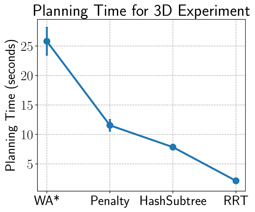
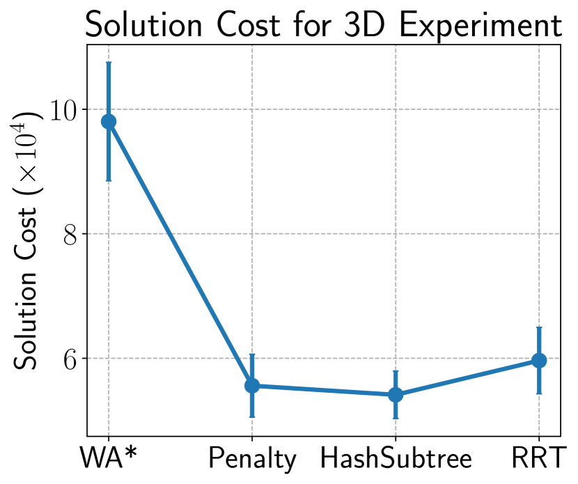
Figure 2: (left) Planning time and (right) Solution cost for 3D experiment. Error bars show standard error over $30$ runs.

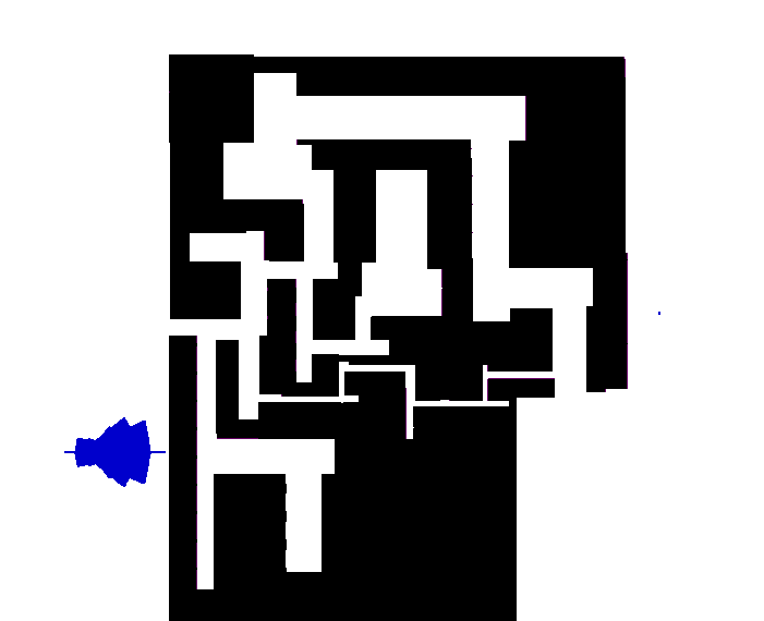
(a) WA*

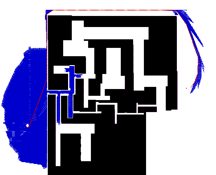
(b) Penalty

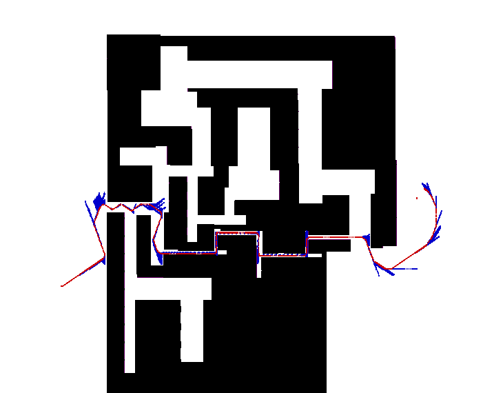
(c) Subtree

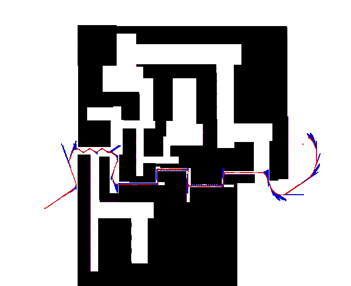
(d) HashSubtree

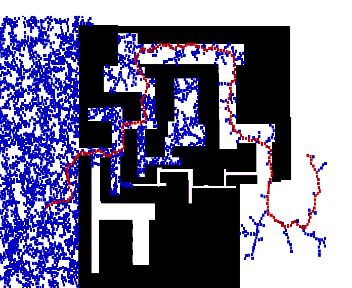
(e) RRT

Figure 3: Heatmaps showing results for 3D experiment. The red path shows the solution, and blue regions represent states that have been expanded. In the case of RRT, blue states represent sampled states. The start is to the left of maze and the goal is to the right of maze. All approaches are successful, except for WA* which could not find a solution in $120$ seconds.

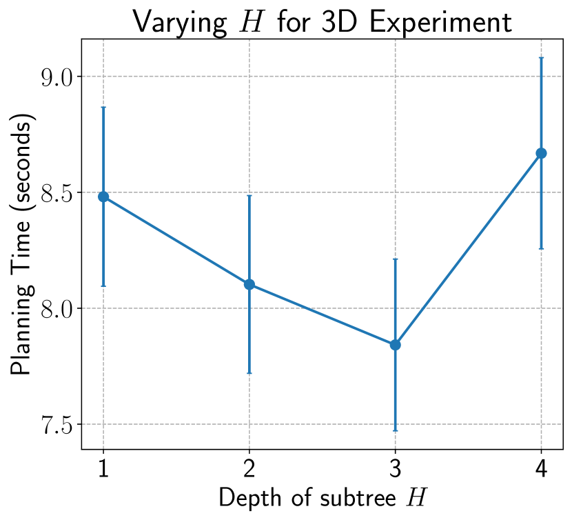
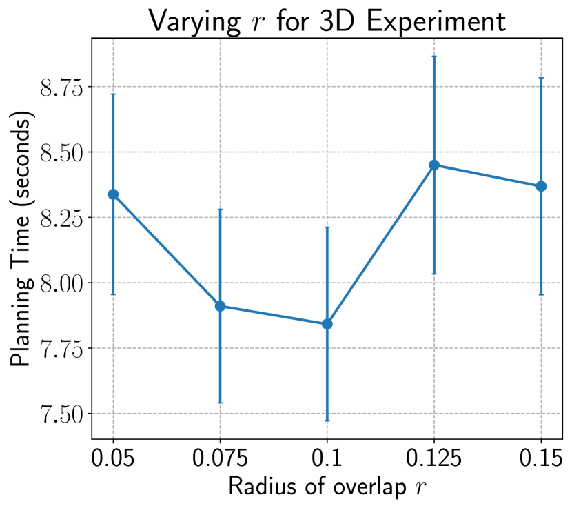
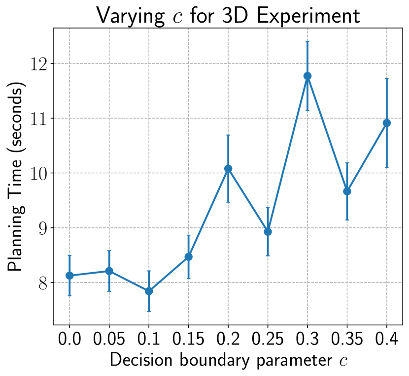
Figure 4: Planning time as the (left) subtree depth $H$, (middle) radius of overlap $r$, and (right) decision boundary parameter $c$ are varied in 3D experiments while keeping the other parameters fixed. Error bars show standard error over $30$ runs.

IV-A 3D Experiment

Our first set of experiments involve a 3D planning domain with a car-like robot. We use $3$ maps from Moving AI lab [23] each with $10$ randomly chosen start and goal pairs. Motion primitives are generated for the robot using a unicycle model with constraints on the turning radius resulting in $5$ successors for each expansion. The state space is specified using $s=(x,y,\theta)$ where $(x,y)$ describe the position of the robot, and $\theta$ describes the heading. We use values of $c$, $H$, and $r$ as the best performing values according to experiments in Section IV-C. We use $\epsilon_{0}=1$, and $\epsilon_{\mathsf{max}}=2$.

The results are presented in Figure 2 and Table I. Figure 2 shows that our approach HashSubtree outperforms both WA* and the state-of-the-art soft duplicate detection Penalty in planning time by more than a factor of $1.5$, without sacrificing solution cost (in fact, computes better solutions.) RRT outperforms HashSubtree in planning time but computes solutions with higher costs which is typical of sampling-based planners that provide no guarantees on sub-optimality of solution. The reason for the success of our approach is illustrated in the example shown in Figure 3. Our approaches Subtree and HashSubtree compute the solution with significantly less number of expansions when compared to other approaches. Since expansions are the most expensive operation in search, reducing the number of expansions leads to large savings in planning time.

Table I emphasizes the impact of using subtree overlap metric in duplicity computation. We observe that Subtree that constructs subtrees and computes subtree overlap during search achieves least expansions during search, not counting the additional expansions for subtree construction. However, as described in Section III-D, Subtree takes a long time to compute a solution because of these additional expansions, and HashSubtree avoids this by precomputing subtree overlap values offline and using the stored values during search. It is important to note that HashSubtree incurs a small increase in number of expansions due to discretization, but greatly reduces the planning time when compared to Subtree. Thus, HashSubtree retains the advantages of using subtree overlap metric while achieving fast planning times.

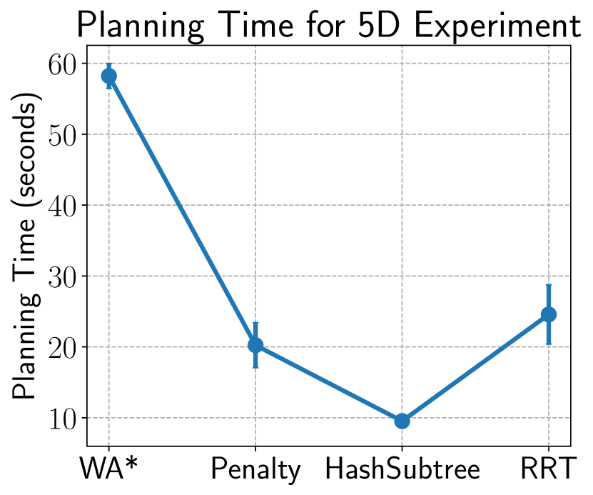
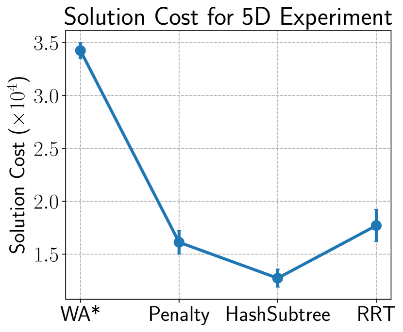
Figure 5: (left) Planning time and (right) Solution cost for 5D experiment. Error bars show standard error over $30$ runs.

IV-B 5D Experiment

Our second set of experiments involve a 5D planning domain with an unmanned aerial vehicle that has constraints on linear acceleration and angular speed. We use $5$ maps that are mesh models of real world with obstacles being no-fly zones each with $6$ randomly chosen start and goal pairs. Computing motion primitives using two point boundary value problem solvers is difficult for this domain. Thus, motion primitives are generated for the robot using a local controller with inputs planar acceleration in $XY$ plane $a_{xy}$, velocity in $Z$ axis $v_{z}$, and the yaw angular speed $\omega$ resulting in $27$ successors for each expansion. The state space is specified using $s=(x,y,z,\theta,v_{xy})$ where $(x,y,z)$ describe the position of the robot, $\theta$ describes the heading, and $v_{xy}$ the velocity in $XY$ plane. We use $\epsilon_{0}=1$, $\epsilon_{\mathsf{max}}=5$, $c=0.5$, $H=1$, and $r=0.1$.

The results are presented in Table I and Figure 5. Figure 5 shows that HashSubtree outperforms other approaches in terms of planning time by more than a factor of $2$. The heuristic computed using only $(x,y,z)$ locations is not as informative in $5$D as it was in $3$D, which results in duplicate detection playing a more important role. Consequently, WA* is only able to solve $1$ of the $30$ runs within $120$ seconds, while Penalty solves all runs but takes twice as long planning times when compared to HashSubtree. RRT also has large planning times as all the maps have narrow passageways that the robot must pass through with highly constrained dynamics, to get to the goal. Thus, RRT uses a lot of samples before it computes a solution leading to large planning times. As expected, the cost of RRT solution is also higher than search-based approaches. Table I shows that Subtree achieves the least expansions during search but has large planning times due to subtree construction, and HashSubtree achieves the best of both worlds with low expansions and least planning time.

IV-C Sensitivity Analysis

The final set of experiments involve the 3D planning domain described before with the same maps, and start and goal pairs. These experiments aim to analyze how sensitive the performance of our approach HashSubtree is to the hyperparameters in the proposed duplicity function $\mathsf{dup}_{\mathcal{S}}$, i.e. depth of subtree $H$, radius of overlap $r$, and decision boundary parameter $c$.

The results are summarized in Figure 4. We observe that the performance of HashSubtree does not vary much with both depth of the subtree $H$, and radius of overlap $r$. Thus, our approach is robust to the choice of these hyperparameters. However, the hyperparameter $c$ plays an important role in the performance of HashSubtree as shown in Figure 4 (right) and needs to be chosen carefully using prior domain knowledge to obtain the best performance. More investigation is needed to understand the best way to automatically chose this hyperparameter, and is left for future work.

V Conclusions and Future Work

We presented a soft duplicate detection approach for search-based planning methods to operate in continuous spaces. Unlike previous work [1] that uses a simple metric based on euclidean distance to compute the duplicity of a state, we introduce a more kinodynamically informed metric, namely subtree overlap, that encodes the likelihood of a state contributing to the solution given that the search has already seen other states. Theoretically, we show that our approach has completeness and sub-optimality bound guarantees using weighted A* and the proposed duplicity function. Empirically, our approach outperforms previous approaches in terms of planning time by a factor of $1.5$ to $2\times$ on $3$D and $5$D planning domains with highly constrained dynamics. One direction for future work would be to explore automatically selecting the decision boundary parameter $c$ given a new planning domain. Furthermore, while HashSubtree outperformed other approaches in terms of planning time in $3$D and $5$D domains, it is infeasible to store subtree overlap values in a hashtable for higher dimensional planning domains as the size of the hashtable grows exponentially. A potential solution is to train a function approximator offline to learn to predict subtree overlap $\eta_{H}(s,s^{\prime})$ given feature representations of the states $s,s^{\prime}$. The trained function approximator can be used during search to quickly compute the duplicity of a state in high dimensional planning problems.

References

- [1] W. Du, S. Kim, O. Salzman, and M. Likhachev, “Escaping local minima in search-based planning using soft duplicate detection,” in 2019 IEEE/RSJ International Conference on Intelligent Robots and Systems, IROS 2019, Macau, SAR, China, November 3-8, 2019. IEEE, 2019, pp. 2365–2371. [Online]. Available: https://doi.org/10.1109/IROS40897.2019.8967815
- [2] D. Berenson, S. S. Srinivasa, D. Ferguson, and J. J. Kuffner, “Manipulation planning on constraint manifolds,” in 2009 IEEE International Conference on Robotics and Automation, ICRA 2009, Kobe, Japan, May 12-17, 2009. IEEE, 2009, pp. 625–632. [Online]. Available: https://doi.org/10.1109/ROBOT.2009.5152399
- [3] R. E. Allen and M. Pavone, “A real-time framework for kinodynamic planning in dynamic environments with application to quadrotor obstacle avoidance,” Robotics Auton. Syst., vol. 115, pp. 174–193, 2019. [Online]. Available: https://doi.org/10.1016/j.robot.2018.11.017
- [4] K. K. Hauser, T. Bretl, K. Harada, and J. Latombe, “Using motion primitives in probabilistic sample-based planning for humanoid robots,” in Algorithmic Foundation of Robotics VII, Selected Contributions of the Seventh International Workshop on the Algorithmic Foundations of Robotics, WAFR 2006, July 16-18, 2006, New York, NY, USA, ser. Springer Tracts in Advanced Robotics, S. Akella, N. M. Amato, W. H. Huang, and B. Mishra, Eds., vol. 47. Springer, 2006, pp. 507–522. [Online]. Available: https://doi.org/10.1007/978-3-540-68405-3“˙32
- [5] S. Liu, N. Atanasov, K. Mohta, and V. Kumar, “Search-based motion planning for quadrotors using linear quadratic minimum time control,” in 2017 IEEE/RSJ International Conference on Intelligent Robots and Systems, IROS 2017, Vancouver, BC, Canada, September 24-28, 2017. IEEE, 2017, pp. 2872–2879. [Online]. Available: https://doi.org/10.1109/IROS.2017.8206119
- [6] M. Pivtoraiko and A. Kelly, “Kinodynamic motion planning with state lattice motion primitives,” in 2011 IEEE/RSJ International Conference on Intelligent Robots and Systems, IROS 2011, San Francisco, CA, USA, September 25-30, 2011. IEEE, 2011, pp. 2172–2179. [Online]. Available: https://doi.org/10.1109/IROS.2011.6094900
- [7] B. J. Cohen, S. Chitta, and M. Likhachev, “Search-based planning for manipulation with motion primitives,” in IEEE International Conference on Robotics and Automation, ICRA 2010, Anchorage, Alaska, USA, 3-7 May 2010. IEEE, 2010, pp. 2902–2908. [Online]. Available: https://doi.org/10.1109/ROBOT.2010.5509685
- [8] M. Pivtoraiko, R. A. Knepper, and A. Kelly, “Differentially constrained mobile robot motion planning in state lattices,” J. Field Robotics, vol. 26, no. 3, pp. 308–333, 2009. [Online]. Available: https://doi.org/10.1002/rob.20285
- [9] S. M. LaValle, Planning Algorithms. Cambridge University Press, 2006. [Online]. Available: http://planning.cs.uiuc.edu/
- [10] R. Bellman, “Dynamic programming and stochastic control processes,” Inf. Control., vol. 1, no. 3, pp. 228–239, 1958. [Online]. Available: https://doi.org/10.1016/S0019-9958(58)80003-0
- [11] S. M. LaValle and J. J. K. Jr., “Randomized kinodynamic planning,” Int. J. Robotics Res., vol. 20, no. 5, pp. 378–400, 2001. [Online]. Available: https://doi.org/10.1177/02783640122067453
- [12] S. Karaman and E. Frazzoli, “Sampling-based algorithms for optimal motion planning,” Int. J. Robotics Res., vol. 30, no. 7, pp. 846–894, 2011. [Online]. Available: https://doi.org/10.1177/0278364911406761
- [13] B. Sakcak, L. Bascetta, G. Ferretti, and M. Prandini, “Sampling-based optimal kinodynamic planning with motion primitives,” Auton. Robots, vol. 43, no. 7, pp. 1715–1732, 2019. [Online]. Available: https://doi.org/10.1007/s10514-019-09830-x
- [14] J. Mainprice, N. D. Ratliff, M. Toussaint, and S. Schaal, “An interior point method solving motion planning problems with narrow passages,” in 29th IEEE International Conference on Robot and Human Interactive Communication, RO-MAN 2020, Naples, Italy, August 31 - September 4, 2020. IEEE, 2020, pp. 547–552. [Online]. Available: https://doi.org/10.1109/RO-MAN47096.2020.9223504
- [15] M. Likhachev and A. Stentz, “R* search,” in Proceedings of the Twenty-Third AAAI Conference on Artificial Intelligence, AAAI 2008, Chicago, Illinois, USA, July 13-17, 2008, D. Fox and C. P. Gomes, Eds. AAAI Press, 2008, pp. 344–350. [Online]. Available: http://www.aaai.org/Library/AAAI/2008/aaai08-054.php
- [16] F. Islam, O. Salzman, and M. Likhachev, “Online, interactive user guidance for high-dimensional, constrained motion planning,” in Proceedings of the Twenty-Seventh International Joint Conference on Artificial Intelligence, IJCAI 2018, July 13-19, 2018, Stockholm, Sweden, J. Lang, Ed. ijcai.org, 2018, pp. 4921–4928. [Online]. Available: https://doi.org/10.24963/ijcai.2018/683
- [17] S. Vats, V. Narayanan, and M. Likhachev, “Learning to avoid local minima in planning for static environments,” in Proceedings of the Twenty-Seventh International Conference on Automated Planning and Scheduling, ICAPS 2017, Pittsburgh, Pennsylvania, USA, June 18-23, 2017, L. Barbulescu, J. Frank, Mausam, and S. F. Smith, Eds. AAAI Press, 2017, pp. 572–576. [Online]. Available: https://aaai.org/ocs/index.php/ICAPS/ICAPS17/paper/view/15747
- [18] J. Barraquand and J. Latombe, “Nonholonomic multibody mobile robots: Controllability and motion planning in the presence of obstacles,” Algorithmica, vol. 10, no. 2-4, pp. 121–155, 1993. [Online]. Available: https://doi.org/10.1007/BF01891837
- [19] J. P. Gonzalez and M. Likhachev, “Search-based planning with provable suboptimality bounds for continuous state spaces,” in Proceedings of the Fourth Annual Symposium on Combinatorial Search, SOCS 2011, Castell de Cardona, Barcelona, Spain, July 15.16, 2011, D. Borrajo, M. Likhachev, and C. L. López, Eds. AAAI Press, 2011. [Online]. Available: http://www.aaai.org/ocs/index.php/SOCS/SOCS11/paper/view/4015
- [20] P. A. Dow and R. E. Korf, “Duplicate avoidance in depth-first search with applications to treewidth,” in IJCAI 2009, Proceedings of the 21st International Joint Conference on Artificial Intelligence, Pasadena, California, USA, July 11-17, 2009, C. Boutilier, Ed., 2009, pp. 480–485. [Online]. Available: http://ijcai.org/Proceedings/09/Papers/087.pdf
- [21] I. Pohl, “Heuristic search viewed as path finding in a graph,” Artif. Intell., vol. 1, no. 3, pp. 193–204, 1970. [Online]. Available: https://doi.org/10.1016/0004-3702(70)90007-X
- [22] J. L. Bentley, “Multidimensional binary search trees used for associative searching,” Commun. ACM, vol. 18, no. 9, pp. 509–517, 1975. [Online]. Available: http://doi.acm.org/10.1145/361002.361007
- [23] N. R. Sturtevant, “Benchmarks for grid-based pathfinding,” IEEE Trans. Comput. Intell. AI Games, vol. 4, no. 2, pp. 144–148, 2012. [Online]. Available: https://doi.org/10.1109/TCIAIG.2012.2197681