Optimizing Age-of-Information in Adversarial Environments with Channel State Information

Abstract

This paper considers a multi-user downlink scheduling problem with access to the channel state information at the transmitter (CSIT) to minimize the Age-of-Information (AoI) in a non-stationary environment. The non-stationary environment is modelled using a novel adversarial framework. In this setting, we propose a greedy scheduling policy, called MA-CSIT, that takes into account the current channel state information. We establish a finite upper bound on the competitive ratio achieved by the MA-CSIT policy for a small number of users and show that the proposed policy has a better performance guarantee than a recently proposed greedy scheduler that operates without CSIT. In particular, we show that access to the additional channel state information improves the competitive ratio from $8$ to $2$ in the two-user case and from $18$ to $\nicefrac{{8}}{{3}}$ in the three-user case. Finally, we carry out extensive numerical simulations to quantify the advantage of knowing CSIT in order to minimize the Age-of-Information for an arbitrary number of users.

I Introduction

In addition to throughput, delay, and spectral efficiency, the Age-of-Information (AoI) metric has recently emerged as one of the key determinants of the Quality of Service (QoS) offered by the next-generation wireless networks. The AoI metric, first introduced in [1], measures the freshness of information available to the users in real-time. Ever since the pioneering work by Kaul et al., there has been an extensive body of work on optimizing and understanding the design implications of AoI in communication systems. See [2] for a comprehensive introduction to the recent advances in this area. In order to keep the analysis tractable, most of the existing papers on AoI assume stationary stochastic system models [3, 4]. Furthermore, the usual performance guarantees given in the literature in connection with AoI are almost always asymptotic in nature. On the contrary, applications where the AoI metric is critical to the system performance, such as the ultra-reliable low latency communication (URLLC) and mission-critical communication in cyber-physical systems, typically operate far from the stationary regime [5]. For acceptable performance, these applications also require stringent non-asymptotic upper limits on the age-of-information. To address this issue, in this paper, we focus on designing robust scheduling algorithms that ensure the maximum information freshness for the end-users, irrespective of the possibly time-varying statistics of the underlying wireless channel. In our recent papers [6, 7, 8], we introduced an adversarial version of Binary Erasure Channel (BEC) model, and showed that a greedy scheduling policy is approximately competitively optimal. These papers assume that the channel states are adversarially chosen and the scheduler does not have access to the current channel state information (CSIT). In the present paper, we extend our previous results to the setting where the channel state information of the current slot is available to the scheduler. The main objective of this paper is to quantify the provable improvement in performance due to the availability of CSIT compared to the setting when the transmitter is oblivious to the current channel state. Due to the complexity of the analysis, we only have been able to theoretically analyze the setting when the number of users ($N)$ is either two or three. Our numerical experiments suggest the AoI advantage continues in the presence of CSIT even when the number of users is large. We anticipate that the tools and techniques developed in this paper will be useful to tackle the general problem with an arbitrary number of users. In this paper, we claim the following two main contributions:

1. For the adversarial channel model, we establish an improved upper bound on the competitive ratio for a greedy online scheduling policy that has access to the current CSIT. We show that the proposed online policy is 2-competitive when $N=2$ and $\nicefrac{{8}}{{3}}\sim 2.67$-competitive when $N=3$. This improves the previously known tight upper-bounds on the competitive ratios (without CSIT), which are known to be $8$ (for $N=2$) and $18$ (for $N=3$) respectively (see Theorem 3 of [9] and Theorem 1 of [8], where the competitive ratio is bounded by $2N^{2}$ for any $N\geq 1$).

2. We numerically compare the performance of the online scheduling policy which knows channel states at the current slot with a greedy online scheduling policy which does not have the current channel state information. Our results show that the AoI is substantially reduced with CSIT.

The rest of the paper is organized as follows. In Section II, we describe our adversarial system model and formulate the problem. In Section III, we derive the competitive ratio of a greedy scheduling policy for the case $N=2$ and $N=3$. In Section IV, we present our simulation results, and finally, in Section VI, we conclude the paper with a brief discussion on possible future research directions.

II System Model and Problem Formulation

We consider an online scheduling problem with $N$ users located in the coverage area of a single Base Station (henceforth referred to as BS). Time is slotted, and at the beginning of every slot, a fresh update packet arrives at the BS from some external source. Such traffic models are known as the saturated traffic models in the literature [10, 11, 12]. Each of the $N$ users are interested in receiving the fresh packet at each slot to keep up-to-date with the external source. Once a fresh packet arrives, the BS beamforms and schedules a packet transmission to one of the $N$ users according to a scheduling policy $\pi$. The downlink channels from the BS to the users are assumed to be non-stationary, modeled as an adversarial binary erasure channel, whose states are dictated by an adversary. In particular, the downlink channel state for any user could be either Good or Bad as determined by the adversary. The online scheduling policy $\pi$, equipped with the channel state information (CSIT), knows the current channel states of all users before the scheduling decision for a slot is made. Making use of the current channel state information, the policy selects a user having a Good channel (if any) and then transmits the latest packet from the BS to the user. The adversary controlling the channel states may know the scheduling policy as well. This adversarial framework was first introduced in our recent papers [6, 7, 8].

Our objective is to design a scheduling policy that competitively optimizes the average freshness of information for all the users. For any time slot $t\geq 1$, let $t_{i}(t)$ denotes the last time slot when the $i^{th}$ user successfully received a packet from the BS. The Age of Information (AoI) for the $i^{th}$ user at slot $t$ is defined as:

$$h_{i}(t)=t-t_{i}(t).$$

In other words, the quantity $h_{i}(t)$ measures the number of time slots before which the $i^{th}$ user received the last packet prior to time $t$. The $N$ dimensional vector $\bm{h}(t)$ represents the collection of AoI for $N$ users at time $t$ where $i^{th}$ element of the vector refers to the AoI of the $i^{th}$ user i.e. $h_{i}(t)$. The age $h_{i}(t)$ increases linearly with time until the $i^{th}$ user receives a fresh packet. Once a user receives a fresh packet, its AoI instantaneously drops to unity. See Fig. 1 for an illustration of the evolution of AoI.

Objective function

Throughout this paper, we consider optimizing the total AoI metric, which is defined as the sum of AoI cost incurred for all users over the entire time horizon under consideration. Hence, the objective function for the AoI minimization can be expressed as:

$$\textrm{AoI}(T)=\sum_{t=1}^{T}(\sum_{i=1}^{T}h_{i}(t))$$ (1)

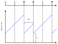
Figure 1: Time evolution of $h_{i}(t)$, an arrow indicates successful transmission of fresh packet to the $i^{th}$ user.

II-A Performance metric

To quantify the performance of any scheduling policy, we use the standard notion of competitive ratio from the online algorithms literature [13, 14]. To be specific, the competitive ratio of any online policy $\pi$ is defined as the ratio between worst-case cost incurred by the policy $\pi$ and the cost incurred by the offline clairvoyant optimal policy OPT, which knows the entire sequence of channel states in advance. Let $\sigma$ denote any sequence of channel states. The competitive ratio of an online policy $\pi$ can be expressed as:

$$\eta^{\pi}=\sup_{\sigma}\Bigg{(}\frac{\text{Cost of the policy $\pi$ on $\sigma$}}{\text{Cost of {OPT} on $\sigma$}}\Bigg{)},$$ (2)

where, in the above, the supremum is taken over all possible finite length channel state sequences $\sigma$.

II-B Scheduling Policies

In this paper we analyze the performance of the following online policy:

Max-Age with CSIT policy (MA-CSIT)

At each time slot, the scheduler determines the current channel states of all users using the CSIT. The BS then schedules a fresh packet transmission to the user having the highest age among all users currently having a Good channel. If at any time slot, no channel is in Good state, the MA-CSIT policy does not schedule a packet transmission to any user.

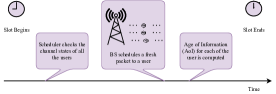
Figure 2: Timeline of MA-CSIT policy at a particular time slot

For bounding the competitive ratio of the MA-CSIT policy, we need to characterize the Offline optimal policy (OPT). The OPT policy is assumed to know the channel states of all the users for the entire time duration a priori. Hence, the performance of any other scheduling policy is dominated by that of OPT. However, the OPT policy can not be implemented in an online fashion as it assumes the knowledge of the future channel states.

Baseline

In order to determine the benefit of having CSIT, we compare the performance of the MA-CSIT policy with the Max-Age policy that does not consider the channel state information [6, 8]. Under the Max-Age policy, at each time slot $t$, BS schedules a fresh packet to the user which has the highest age among all the users, irrespective of the current channel states. Hence, if the channel state at the scheduled user-end turns out to be Bad, the packet is lost.

III Performance Analysis

In this section, we bound the competitive ratio of the MA-CSIT policy from the above.

A note on determining the Max-age users

To begin with, at any time slot, we first sort the users according to descending order of their ages under the MA-CSIT policy. The user, who has the highest age among all the users (under the MA-CSIT policy) is called the Max-age user (ties are broken arbitrarily). Similarly, the $m^{th}$ user in the sorted list is called the $m^{th}$ Max-age user. Thus the Max-age user corresponds to $m=1$ in the sorted list at that time slot. Naturally, under a different policy (e.g., OPT) the Max-Age user may not have the highest age among all users.

Next, we recall the concept of a time interval, first introduced in [9],

Definition 1

(Interval) A new interval is said to begin when the Max-age user transmits a packet successfully under the MA-CSIT policy.

Hence, an interval continues until the channel corresponding to the Max-age user becomes $Good$. Let the quantity $h_{k}^{i,t}$ denote the age of the $k^{th}$ user at the $t$^th time slot of the $i$^th interval under the MA-CSIT policy. Also, let $o_{k}^{i,t}$ denote the age of the $k^{th}$ user at the $t^{th}$ time slot of $i^{th}$ interval under OPT policy. So $h_{k}^{i,1}$ denotes the age of the $k^{th}$ user at the first time slot of the $i^{th}$ interval under the MA-CSIT policy. The length of the $i^{th}$ interval is denoted as $I_{i}$ and the total AoI cost incurred by the MA-CSIT and the OPT policies on the $i$^th interval are denoted by $C_{\textsf{MA-CSIT}}(I_{i})$ and $C_{\textsf{OPT}}(I_{i})$ respectively. With the above definitions in place, we now proceed to bound the competitive ratio of the MA-CSIT policy.

III-A Competitive ratio of the MA-CSIT policy for $N=2$ users

Proposition 1

The competitive ratio of the MA-CSIT policy for $N=2$ users is upper bounded as $\eta^{\textsf{MA-CSIT}}\leq 2$.

Proof:

For two users, we can express the difference between the costs incurred by the MA-CSIT policy and OPT as:

$$C_{\textsf{MA-CSIT}}(I_{i})-C_{\textsf{OPT}}(I_{i})=\sum_{t}(h_{1}^{i,t}-o_{1}^{i,t})+\sum_{t}(h_{2}^{i,t}-o_{2}^{i,t}),$$ (3)

where the index in the summation ranges over all slots in the $i$^th interval. We now establish the following Lemma.

Lemma 1

For the Max-age user, the age difference between the MA-CSIT policy and the OPT policy for every time slot $t$ of $i^{th}$ interval remains constant. For example, if at the $i^{th}$ interval the user 1 remains the Max-age user then the age difference $(h_{1}^{i,t}-o_{1}^{i,t})$ remains constant throughout the interval $i$.

Proof:

Without any loss of generality, let us assume that the MA-CSIT policy serves the user 2 at the beginning of the $i^{th}$ interval, and at the $i^{th}$ interval, the user 1 becomes the Max-age user.
We establish Lemma 1 on the basis of the following observation. Both MA-CSIT and OPT policies can not serve the Max-age user until the channel corresponding to that user becomes Good. Furthermore, whenever the channel becomes $Good$, the MA-CSIT policy will serve the Max-age user immediately and a new interval begins. Thus, within any interval, both the quantities $h_{1}^{i,t}$ and $o_{1}^{i,t}$ increase linearly. Hence,

$$h_{1}^{i,t}-o_{1}^{i,t}=h_{1}^{i,1}-o_{1}^{i,1}\quad\forall t.$$ (4)

∎

Since we assume that user 1 is the Max-age user at the $i^{th}$ interval, we have $h_{1}^{i,1}>h_{2}^{i,1}$. The next interval, i.e., the $(i+1)^{th}$ interval begins when the MA-CSIT policy serves user 1. Thus we have,

$$C_{\textsf{MA-CSIT}}(I_{i})=C_{\textsf{OPT}}(I_{i})+(h_{1}^{i,1}-o_{1}^{i,1})I_{i}+\sum_{t}(h_{2}^{i,t}-o_{2}^{i,t})$$ (5)

We now establish the following useful result.

Lemma 2

For the user other than the Max-age user, the age difference between the MA-CSIT and the OPT policy is always non-positive (i.e., $h_{2}^{i,t}-o_{2}^{i,t}\leq 0,\forall t$ for this case).

Proof:

To prove $h_{2}^{i,t}-o_{2}^{i,t}\leq 0$ $\forall t$ we use the following facts. At the next time slots of the $i^{th}$ interval whenever the channel corresponding to user 2 becomes $Good$, both the MA-CSIT and the OPT policies serve the user 2. The only scenario when the age of user 2 under the MA-CSIT policy becomes greater than age of user 2 under OPT i.e. $h_{2}^{i,t}>o_{2}^{i,t}$ is when the channel corresponding to user 2 becomes $Good$ and OPT serves the user 2 but MA-CSIT does not. In other words the OPT policy serves the user 2 while the MA-CSIT policy serves the user 1. Since we considered user 1 as the Max-age user and if the MA-CSIT policy serves the user 1, from the definition of interval the next interval i.e. $(i+1)^{th}$ interval starts. This implies at the $i^{th}$ interval the age of the user 2 under MA-CSIT will never become more than the age under OPT. Hence,

$$h_{2}^{i,t}-o_{2}^{i,t}\leq 0\quad\forall t$$ (6)

∎

Combining the above two Lemmas, equation (3) may be simplified as

$$C_{\textsf{MA-CSIT}}(I_{i})\leq C_{\textsf{OPT}}(I_{i})+(h_{1}^{i,1}-o_{1}^{i,1})I_{i}$$ (7)

For bounding the second term in the above inequality, we need to introduce the notion of Residue-Length as defined below:

Definition 2

(Residue-length) The $i^{th}$ residue-length $l_{i}$ is the length of time from the last slot in the previous interval when the Max-age user of the $i^{th}$ interval got served by the MA-CSIT policy, counted up to the beginning of the $i^{th}$ interval.

See Fig. 3 for an illustration of the intervals and the residue lengths. It is not hard to verify that the difference of the ages of the Max-age user under the MA-CSIT policy and OPT at the beginning of the $i^{th}$ interval can be upper bounded by the residue-length $l_{i}$ i.e. $h_{1}^{i,1}-o_{1}^{i,1}\leq l_{i}$. Hence, from Eqn. (7), we have the following upper bound:

$$C_{\textsf{MA-CSIT}}(I_{i})\leq C_{\textsf{OPT}}(I_{i})+l_{i}I_{i}.$$ (8)

Finally, to find an upper bound to the competitive ratio, we need to derive a lower bound of the cost of the OPT policy for each intervals. Note that, after the first time slot of any interval, the Max-age user, by definition, encounters consecutive $Bad$ channels. Hence, the cost corresponding to that user under the OPT policy can be lower bounded by $\sum_{k=1}^{I_{i}}k$.

During the $i$^th interval, the channel corresponding to the user other than the Max-age user (i.e. user 2) does not become $Good$ after the $(I_{i}-l_{i+1})$^th time slot. This fact can be verified from the definition of residue-length. Therefore, the cost for user 2 under OPT for the $i$^th interval can be lower bounded as:

$$\sum_{k=1}^{I_{i}-l_{i+1}}1+\sum_{k=1}^{l_{i+1}}k=I_{i}-l_{i+1}+\sum_{k=1}^{l_{i+1}}k.$$ (9)

Hence, the total AoI cost under the OPT policy (including both users) for the $i$^th interval can be lower bounded as:

$$C_{\textsf{OPT}}(I_{i})\geq\sum_{k=1}^{I_{i}}k+I_{i}-l_{i+1}+\sum_{k=1}^{l_{i+1}}k.$$ (10)

Summing up the costs over all intervals we have the following bound:

$$\sum_{i}C_{\textsf{MA-CSIT}}(I_{i})\leq\sum_{i}C_{\textsf{OPT}}(I)+\sum_{i}l_{i}I_{i}.$$ (11)

Substituting the bound from Eqn. (10) in the inequality above, we have:

$$\frac{\sum_{i}C_{\textsf{MA-CSIT}}(I_{i})}{\sum_{i}C_{\textsf{OPT}}(I_{i})}\leq 1+\frac{\sum_{i}l_{i}I_{i}}{\sum_{i}(\sum_{k=1}^{I_{i}}k+I_{i}-l_{i+1}+\sum_{k=1}^{l_{i+1}}k)}.$$ (12)

Now we use the AM-GM inequality to get $l_{i}I_{i}\leq\frac{l_{i}^{2}}{2}+\frac{I_{i}^{2}}{2}$.
Furthermore, we have $\sum_{k=1}^{I_{i}}k+I_{i}-l_{i+1}+\sum_{k=1}^{l_{i+1}}k=\frac{I_{i}(I_{i}+1)}{2}+I_{i}+\frac{(l_{i+1})(l_{i+1}+1)}{2}-l_{i+1}\geq\frac{I_{i}^{2}}{2}+\frac{l_{i+1}^{2}}{2}$.
Hence,

$$\frac{\sum_{i}C_{\textsf{MA-CSIT}}(I_{i})}{\sum_{i}C_{\textsf{OPT}}(I_{i})}\leq 1+\frac{\sum_{i}\frac{l_{i}^{2}}{2}+\frac{I_{i}^{2}}{2}}{\sum_{i}\frac{I_{i}^{2}}{2}+\frac{l_{i+1}^{2}}{2}}\leq 2,$$ (13)

where we have used the fact that, by definition $l_{1}=0.$ Hence, $\eta^{\textsf{MA-CSIT}}\leq 2$. ∎

The above result should be compared and contrasted with Theorem 3 of [8], which proves an upper limit of $8$ for the competitive ratio of the Max-Age policy that operates without CSIT.
In the following, we extend the above proof technique for $N=3$ users. The reader will find that although the basic line of analysis remains the same, the details become much more involved in this case.

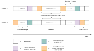
Figure 3: Illustration of residue length and interval construction for 2 users. Channel $i$ refers to the state of the channel corresponding to user $i$.

III-B Competitive ratio of the MA-CSIT policy for $N=3$ users

Proposition 2

The competitive ratio of MA-CSIT policy for $N=3$ users is upper bounded as $\eta^{\textsf{MA-CSIT}}\leq\frac{8}{3}.$

Proof: We use the same definition of intervals as in our previous proof. The difference in the AoI costs incurred by the MA-CSIT and the OPT policies can be expressed as follows:

$$C_{\textsf{MA-CSIT}}(I_{i})-C_{\textsf{OPT}}(I_{i}) \ =\sum_{t}(h_{1}^{i,t}-o_{1}^{i,t})+\sum_{t}(h_{2}^{i,t}-o_{2}^{i,t})+$$

$$\ \sum_{t}(h_{3}^{i,t}-o_{3}^{i,t}),$$ (14)

where the index in the summation ranges over all slots in the $i$^th interval. Without any loss of generality, let us assume that user 1 is the Max-age user for the $i^{th}$ interval under the MA-CSIT policy. Note that Lemma 1 holds for any number of users (hence, for $N=3$ also). This is because whenever the channel corresponding to the Max-age user becomes $Good$, the MA-CSIT policy serves that user immediately and a new interval begins. Thus, the difference of ages of the Max-age user under the MA-CSIT and OPT policies remains constant throughout any interval (as both increase linearly throughout an interval). Therefore we can write

$$C_{\textsf{MA-CSIT}}(I_{i}) \ =C_{\textsf{OPT}}(I_{i})+(h_{1}^{i,1}-o_{1}^{i,1})I_{i}+\sum_{t}(h_{2}^{i,t}-o_{2}^{i,t})+$$

$$\ \sum_{t}(h_{3}^{i,t}-o_{3}^{i,t}).$$ (15)

Using the same definition of residue-lengths as before, we can express the above difference as:

$$C_{\textsf{MA-CSIT}}(I_{i})=C_{\textsf{OPT}}(I_{i})+l_{i}I_{i}+\sum_{t}(h_{2}^{i,t}-o_{2}^{i,t})+\sum_{t}(h_{3}^{i,t}-o_{3}^{i,t}).$$ (16)

We denote the time slot when the Max-age user of the $i$^th interval got served by the MA-CSIT policy as $T_{l_{i}}$.
To upper bound the quantity $\sum_{t}(h_{2}^{i,t}-o_{2}^{i,t})+\sum_{t}(h_{3}^{i,t}-o_{3}^{i,t})$ we introduce the notion of sub-intervals, which form a partition of the intervals. The formal definition of a sub-interval is given below:

Definition 3

(Sub-interval) Within an interval, a new sub-interval is said to begin when the MA-CSIT policy serves the $2^{nd}$ Max-age user among the three users.

Let, $J_{i}$ denotes the number of sub-intervals in the $i$^th interval.
We define the $j^{th}$ Sub-Residue length of the $i^{th}$ interval, $l^{i}_{j}$ as follows:

Definition 4

(Sub-Residue length) The $j^{th}$ sub-residue length of the $i^{th}$ interval (denoted by $l^{i}_{j}$) is the time-elapsed since the last time slot when the $2$^nd Max-age user of the $j$^th sub-interval of the $i$^th interval got served by the MA-CSIT policy, up to the beginning of the $(j+1)$^th sub-interval.

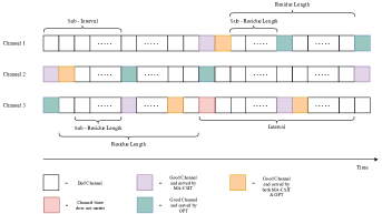
Figure 4: Illustration of residue length and interval construction for 3 users. Channel $i$ refers to the state of the channel corresponding to user $i$.

We illustrate the notion of sub-intervals and sub-residue lengths in Fig. 4. Note that, the above definition is analogous to the definition of intervals.

In every sub-interval, the age of user which has the least age under MA-CSIT policy would be always upper bounded by age of that user under the OPT policy. It directly follows from Lemma 2, discussed in the previous section. Hence, we have the following upper bound:

$$C_{\textsf{MA-CSIT}}(I_{i})\leq C_{\textsf{OPT}}(I_{i})+l_{i}I_{i}+\sum_{j}l^{i}_{j}I^{i}_{j}$$ (17)

where $I^{i}_{j}$ refers to the length of the $j^{th}$ sub-interval of the $i^{th}$ interval, and the index $j$ runs over all sub-intervals of the $i$^th interval.

Next, we proceed to lower bound the cost incurred by the OPT policy during the $i$^th interval.

Lower bounding the cost of the Max-age user

Since, the $i^{th}$ interval continues until the channel corresponding to the Max-age user becomes $Good$, the cost incurred by the Max-age user (i.e. user 1 in this case) under the OPT policy is lower bounded by

$$\sum_{k=1}^{I_{i}}k\geq\frac{I_{i}^{2}}{2}$$ (18)

Lower bounding the cost of the $2$^nd Max-age user

The cost incurred by the $2^{nd}$ Max-age user under the OPT policy during the $j^{th}$ sub-interval is $\sum_{k=1}^{I^{i}_{j}}k$. This is true because for the entire duration of the $j$^th sub-interval, the channel corresponding to the $2^{nd}$ Max-age user remains $Bad$.

Lower bounding the cost of the $3$^rd Max-age user

Following the definition of the sub-residue lengths, the quantity $l_{j+1}^{i}$ denotes the last time slot when the MA-CSIT policy serves the $2$^nd Max-age user of the $(j+1)$^th sub-interval, counted from the beginning of the $(j+1)$^th sub-interval. On the $(j+1)$^th sub-interval, the $3$^rd Max-age user of the $j$^th sub-interval becomes the $2$^nd Max-age user. Hence, for the last $l_{j+1}^{i}$ time slots of the $j$^th sub-interval, the cost of the $3$^rd Max-age user of the $j$^th sub-interval under the OPT policy is given by $\sum_{k=1}^{l_{j+1}^{i}}k$.
Thus, the cost under the OPT policy during the $j$^th sub-interval of the $i$^th interval, excluding the cost of the Max-age user is lower bounded by:

$$\sum_{k=1}^{I^{i}_{j}}k+\sum_{k=1}^{I_{j}^{i}-l_{j+1}^{i}}1+\sum_{k=1}^{l_{j+1}^{i}}k\geq\frac{(I_{j}^{i})^{2}}{2}+\frac{(l_{j+1}^{i})^{2}}{2},\forall 1\leq j\leq J_{i}-1.$$

For the last sub-interval of the $i$^th interval, the cost incurred by 3^rd Max-age user under the OPT policy is lower bounded by $\sum_{k=1}^{I_{J_{i}}^{i}}1$ (since at the $J_{i}$^th sub-interval sub-residue length does not exist). Hence the cost incurred by the 2^nd Max-age and the 3^rd Max-age user under the OPT at the $J_{i}^{th}$ sub-interval is lower bounded by

$$\sum_{k=1}^{I_{J_{i}}^{i}}k+\sum_{k=1}^{I_{J_{i}}^{i}}1\geq\frac{(I_{J_{i}}^{i})^{2}}{2}$$ (19)

Finally, summing up the cost over all sub-intervals in the $i$^th interval, we get the following lower bound to the cost incurred by the 2^nd Max-age and the 3^rd Max-age user under the OPT policy:

$$\frac{(I_{J_{i}}^{i})^{2}}{2}+\sum_{j=1}^{J_{i}-1}(\frac{(I_{j}^{i})^{2}}{2}+\frac{(l_{j+1}^{i})^{2}}{2})$$ (20)

where $l_{J_{i}}^{i}$ is the sub-residue length of the last sub-interval of the $i$^th interval and $I_{J_{i}}^{i}$ is the length of the last sub-interval of the $i$^th interval.
There are three scenarios depending on the values $m^{th}$ residue length $\forall m\in\{2,3,...\}$ i.e. $l_{m}$ can take,

• Case 1- $l_{m}\leq I_{m-1}$ ,

• Case 2- $I_{m-2}+I_{m-1}>l_{m}>I_{m-1}$,

• Case 3- $l_{m}\geq I_{m-2}+I_{m-1}$.

Case 1

Consider the first scenario where $l_{m}\leq I_{m-1}$ $\forall m\in\{2,3....\}$. Now consider the Max-age user of $(i+1)^{th}$ interval. The MA-CSIT policy serves the Max-age user $l_{i+1}$ time slots before the beginning of the $(i+1)^{th}$ interval i.e at $T_{l_{i+1}}^{th}$ slot. The OPT policy can serve the Max-age user twice after $T_{l_{i+1}}^{th}$ time slot. Since $l_{i+1}\leq I_{i}$, the OPT policy can serve the Max-age user once at the beginning of $J_{i}^{th}$ sub-interval and next at the beginning of $(i+1)^{th}$ interval. So, the $l_{i+1}$ time slots can be divided into two parts. The first part refers to the sub-residue length of the last sub-interval i.e $l_{J_{i}}^{i}$ and the next one refers to the length of final sub-interval i.e. $I_{J_{i}}^{i}$. Hence we have

$$I_{J_{i}}^{i}+l_{J_{i}}^{i}=l_{i+1}$$ (21)

Let $a_{i}$ denotes the first part of $l_{i}$ and $b_{i}$ refers to the second part. So for the above case we have

$$a_{i+1}=l^{i}_{J_{i}}$$ (22)

$$b_{i+1}=I^{i}_{J_{i}}$$ (23)

Hence the lower bound of the OPT policy at Eq. (20) can be rewritten as

$$\frac{b_{i+1}^{2}}{2}+\sum_{j=1}^{J_{i}-2}(\frac{(I_{j}^{i})^{2}}{2}+\frac{(l_{j+1}^{i})^{2}}{2})+\frac{(I_{J_{i}-1}^{i})^{2}}{2}+\frac{a_{i+1}^{2}}{2}$$ (24)

Since $a_{i+1}=l^{i}_{J_{i}}$ and $b_{i+1}=I^{i}_{J_{i}}$, we can rewrite Eqn. (17) as:

$$C_{\textsf{MA-CSIT}}(I_{i})\leq C_{\textsf{OPT}}(I_{i})+l_{i}I_{i}+\sum_{j=1}^{J_{i}-1}(l^{i}_{j}I^{i}_{j})+a_{i+1}b_{i+1}$$ (25)

Summing the costs over all intervals from Eq. (25) and using the lower bound of the OPT policy for the Max-age user of Eq. (18) and the lower bound for the 2nd Max-age and the 3rd Max-age user of Eq. (24) we get the following bound:

$$\ \frac{\sum_{i}C_{\textsf{MA-CSIT}}(I_{i})}{\sum_{i}C_{\textsf{OPT}}(I_{i})}\leq 1+$$

$$\ \frac{\sum_{i}(l_{i}I_{i})+\sum_{j=1}^{J_{i}-1}(l^{i}_{j}I^{i}_{j})+a_{i+1}b_{i+1})}{\sum_{i}(\frac{I_{i}^{2}}{2}+\frac{b_{i+1}^{2}}{2}+\sum_{j=1}^{J_{i}-2}(\frac{(I_{j}^{i})^{2}}{2}+\frac{(l_{j+1}^{i})^{2}}{2})+\frac{(I_{J_{i}-1}^{i})^{2}}{2}+\frac{a_{i+1}^{2}}{2})}$$ (26)

Using the AM-GM inequality, we have $l_{i}I_{i}\leq\frac{l_{i}^{2}}{2}+\frac{I_{i}^{2}}{2}$, $\sum_{j=1}^{J_{i}-1}(l^{i}_{j}I^{i}_{j})\leq\sum_{j=1}^{J_{i}-1}(\frac{(l_{j}^{i})^{2}}{2}+\frac{(I^{i}_{j})^{2}}{2})$ and $a_{i+1}b_{i+1}\leq\frac{a_{i+1}^{2}}{2}+\frac{b_{i+1}^{2}}{2}$. Hence, from the above, we get

$$\ \frac{\sum_{i}C_{\textsf{MA-CSIT}}(I_{i})}{\sum_{i}C_{\textsf{OPT}}(I_{i})}\leq 1+$$

$$\ \frac{\sum_{i}(\frac{l_{i}^{2}}{2}+\frac{I_{i}^{2}}{2}+\sum_{j=1}^{J_{i}-1}(\frac{(l_{j}^{i})^{2}}{2}+\frac{(I^{i}_{j})^{2}}{2})+\frac{a_{i+1}^{2}}{2}+\frac{b_{i+1}^{2}}{2})}{\sum_{i}(\frac{I_{i}^{2}}{2}+\frac{b_{i+1}^{2}}{2}+\sum_{j=1}^{J_{i}-2}(\frac{(I_{j}^{i})^{2}}{2}+\frac{(l_{j+1}^{i})^{2}}{2})+\frac{(I_{J_{i}-1}^{i})^{2}}{2}+\frac{a_{i+1}^{2}}{2})}$$ (27)

Combining above equations we get

$$\frac{\sum_{i}C_{\textsf{MA-CSIT}}(I_{i})}{\sum_{i}C_{\textsf{OPT}}(I_{i})} \ \leq 2+$$

$$\ \frac{\sum_{i}(l_{i}^{2})}{\sum_{i}({I_{i}}^{2}+2\sum_{j=1}^{J_{i}-1}(\frac{(I^{i}_{j})^{2}}{2}+\frac{(l^{i}_{j+1})^{2}}{2})+b_{i+1}^{2}+a_{i+1}^{2})}$$ (28)

Lower bounding the sub-interval lengths and the sub-residue lengths by zero, from the above, we have

$$\frac{\sum_{i}C_{\textsf{MA-CSIT}}(I_{i})}{\sum_{i}C_{\textsf{OPT}}(I_{i})}\leq 2+\frac{\sum_{i}(l_{i}^{2})}{\sum_{i}({I_{i}}^{2}+b_{i+1}^{2}+a_{i+1}^{2})}$$ (29)

Since, $a_{i}+b_{i}=l_{i},$ using the Cauchy-Schwartz inequality, we have $a_{i}^{2}+b_{i}^{2}\geq l_{i}^{2}/2,\forall i.$ Hence, the RHS of the above equation can be further upper bounded as below:

$$\frac{\sum_{i}C_{\textsf{MA-CSIT}}(I_{i})}{\sum_{i}C_{\textsf{OPT}}(I_{i})}\leq 2+\frac{\sum_{i}(l_{i}^{2})}{\sum_{i}({I_{i}}^{2}+\frac{l_{i+1}^{2}}{2})}$$ (30)

We have $l_{i}\leq I_{i-1}$. Note that the RHS of Eqn. (30) is monotonically increasing for $l_{i}\geq 0$. Hence, we can upper bound the RHS of equation (30) by substituting $l_{i}=I_{i-1}$. Therefore, we get

$$\frac{\sum_{i}C_{\textsf{MA-CSIT}}(I_{i})}{\sum_{i}C_{\textsf{OPT}}(I_{i})}\leq 2+\frac{\sum_{i}(I_{i-1}^{2})}{\sum_{i}({I_{i}}^{2}+\frac{I_{i}^{2}}{2})}\leq\frac{8}{3}$$ (31)

Please see the Appendix section for the proof of Case 2 and Case 3. Hence, for all values of $l_{i}$, we get $\frac{\sum_{i}C_{\textsf{MA-CSIT}}(I_{i})}{\sum_{i}C_{\textsf{OPT}}(I_{i})}\leq\frac{8}{3}$ which implies $\eta^{MA-CSIT}\leq\frac{8}{3}$.

IV Simulation Results

In this section we provide two particular channel configurations for 2 users and 3 users scenario to show the tightness of the bound provided in the III-A and III-B sections.

IV-A $N=2$ users case

Consider the following channel state sequence for 2 users where the whole sequence is divided into intervals of fixed length $\Delta$ where $\Delta$ is even. At the beginning of every interval the channel corresponding to the user 1 is Good and the other channel is Bad. For the next $\frac{\Delta}{2}-2$ slots both channels remain Bad. Next, at the $\frac{\Delta}{2}^{th}$ slot both the channels become Good. After that, at the $(\frac{\Delta}{2}+1)^{th}$ slot, the channel corresponding to user 2 remains Good but other channel becomes Bad. For the next $\frac{\Delta}{2}-2$ slots both channels remain Bad and finally at the $\Delta^{th}$ slot both channels become Good. In Fig. 5 the AoI cost ratio between the MA-CSIT and the OPT policy for this particular channel state configuration has been plotted. It can be seen as interval length grows the cost ratio approaches 2, while in section III-A we showed that for 2 user case the competitive ratio for the MA-CSIT policy is upper bounded by 2.

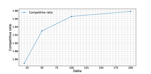
Figure 5: AoI cost comparison between MA-CSIT policy and OPT policy for 2 users

IV-B $N=3$ users case

In this case, we consider the interval length $\Delta$ to be multiple of 6. Here we mention at which time slot the channels corresponding to the users become Good. At the first time slot of the interval the channels corresponding to user 1 and 2 are only Good. For $2^{nd}$ and $3^{rd}$ time slots the channels corresponding user 1 and user 3 remain Good respectively. At the $(\frac{\Delta}{6})^{th}$ time slot, the channels corresponding to user 1 and user 3 become Good and at the next time slot, the channel corresponding to the user 1 only remains Good. After that, at the $(\frac{\Delta}{3}+1)^{th}$ slot, the channels corresponding to user 2 and user 3 become Good. At next two time slots i.e. $(\frac{\Delta}{3}+2)^{th}$ and $(\frac{\Delta}{3}+3)^{th}$ slots the channels corresponding to user 2 and user 1 remain Good respectively. Next at the $\frac{\Delta}{2}^{th}$ time slot the channels corresponding to user 1 and user 2 become Good and at the next time slot, the channel corresponding to user 2 only remains Good. After that at $(\frac{2\Delta}{3}+1)^{th}$ slot, the channels corresponding to user 1 and 3 become Good. For the next two time slots i.e. $(\frac{2\Delta}{3}+2)^{th}$ and $(\frac{2\Delta}{3}+3)^{th}$ slots the channels corresponding to user 3 and user 2 remain Good respectively. Next at $\frac{5\Delta}{6}^{th}$ time slot, the channels corresponding to user 2 and user 3 become Good and at the next time slot, the channel corresponding to user 3 only remains Good. In all other time slots the users which are not mentioned, the channels corresponding to those users remain Bad. For this particular scenario the AoI cost ratio between the MA-CSIT and the OPT policy has been plotted in Fig. 6. As $\Delta$ grows, the cost ratio approaches 2.25, while in section III-B we showed that for 3 user case the competitive ratio for the MA-CSIT policy is upper bounded by 2.67.

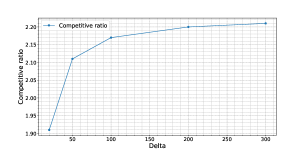
Figure 6: AoI cost comparison between MA-CSIT policy and OPT policy for 3 users

V Comparison between the MA-CSIT and the Max Age policy

In this section we provide numerical results to show the advantage of having CSIT. Through simulations we compare the performance of MA-CSIT policy and the Max-Age policy [6, 8] which does not have CSIT. In this case we consider the channel states corresponding to each user to be independent and identically distributed.

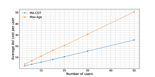
Figure 7: AoI cost comparison between MA-CSIT policy and Max-Age policy

Consider the channel corresponding to each user can be Good with a probability $p$.

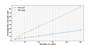
Figure 8: AoI cost comparison between MA-CSIT policy and Max-Age policy

In Fig. 7, Fig. 8 and Fig. 9, the time averaged AoI cost ($AoI_{avg}(T)$) for MA-CSIT policy and Max Age policy when $p=0.5$, $p=0.3$ and $p=0.1$ have been plotted respectively.

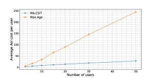
Figure 9: AoI cost comparison between MA-CSIT policy and Max-Age policy

In Fig. 10, the ratio between the average AoI cost of Max Age policy and that of MA-CSIT policy for these three cases has been shown. From the plots we can conclude that when the policy is equipped with CSIT the performance improves drastically.

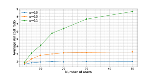
Figure 10: Ratio between AoI cost of MA-CSIT policy and that Max-Age policy

VI Conclusion

The paper investigates the fundamental limits of Age-of-Information for static users over adversarial environments when the scheduling policy is assumed to know the CSIT at the current slot. Theoretically we provide upper bound on the competitive ratio when the number of users is either 2 or 3. Through simulations, we showed that the greedy scheduling policy performs substantially better over adversarial setting when the policy is equipped with the channel state information at the current slot. Finding an upper bound on the competitive ratio for arbitrary number of users is an interesting open problem.

VII Acknowledgement

This work is partially supported by the grant IND-417880 from Qualcomm, USA and a research grant from the Govt. of India for the potential Center-of-Excellence Intelligent Networks under the IoE initiative. The computational results reported in this work were performed on the AQUA Cluster at the High Performance Computing Environment of IIT Madras.

VIII Appendix

Case 2: $I_{m-2}+I_{m-1}>l_{m}>I_{m-1}$

In this case, before the $i^{th}$ interval the last time slot at which the MA-CSIT policy can serve the Max-age user of $i^{th}$ interval would lie somewhere at the $(i-2)^{th}$ interval. At that time slot that user has the least age under the MA-CSIT policy. We denote that time slot as $T_{l_{i}}^{i}$ and the Max-age user of $i^{th}$ interval as $u_{max}^{i}$. Next we need to determine the time slots where the OPT serves $u_{max}^{i}$ but the MA-CSIT does not.

• After $T_{l_{i}}^{i}$ time slot suppose, the OPT serves $u_{max}^{i}$ at some time slot at $(i-2)^{th}$ interval but the MA-CSIT does not. This is only possible when the 2nd Max-age user and $u_{max}^{i}$ get Good channels.Since at the $(i-2)^{th}$ interval, $u^{i}_{max}$ has the least age under the MA-CSIT policy, the MA-CSIT serves the 2nd Max-age user. Hence at that time slot $u_{max}^{i}$ becomes the $2^{nd}$ Max-age user and at the $(i-1)^{th}$ interval it will become the Max-age user. But it is not possible, as $u_{max}^{i}$ is the Max-age user of $i^{th}$ interval and same user can not become Max-age user at two consecutive intervals.

• Another possible scenario is after $T_{l_{i}}^{i}$ the $2^{nd}$ Max-age user at the $(i-2)^{th}$ interval gets Bad channels constantly and at the beginning of $(i-1)^{th}$ interval the channels corresponding to both $u_{max}^{i}$ and the 2nd Max-age user become Good and the OPT serves $u_{max}^{i}$ instead of serving the 2nd Max-age user. In this scenario the MA-CSIT serves the Max-age user and the $2^{nd}$ Max-age user becomes the Max-age user of the $(i-1)^{th}$ interval i.e. $u^{i-1}_{max}$. But in this case the OPT policy can serve $u_{max}^{i-1}$ at max once after the user gets served by the MA-CSIT policy which implies

  $$a_{i-1}=l_{J_{i-1}}^{i-1}=l_{i-1}$$ (32)

  At $T_{l_{i}}^{i}$ time slot the OPT policy can serve either 2nd Max-age user or the $u^{i}_{max}$. But if the OPT policy serves the $u^{i}_{max}$, then for the rest of the time slots of $(i-2)^{th}$ interval and entire $(i-1)^{th}$ interval the cost difference for that user under the OPT and the MA-CSIT policy remains zero.
  Suppose the OPT policy serves the 2nd Max-age user. Since after $T_{l_{i}}^{i}$ time slot, both $u^{i}_{max}$ and 2nd Max-age user get Bad channels constantly and $l^{i-1}_{J_{i-1}}\leq I^{i-1}_{J_{i-1}-1}$ , the cost difference between the MA-CSIT and the OPT policy for the users other than the Max-age user for rest of the $(i-2)^{th}$ interval

  $$l^{i-1}_{J_{i-1}}I^{i-1}_{J_{i-1}}-I^{i-1}_{J_{i-1}-1}I^{i-1}_{J_{i-1}}\leq 0$$ (33)

  Hence the cost difference between the MA-CSIT policy and the OPT policy at $(i-2)^{th}$ interval is

  $$C_{\textsf{MA-CSIT}}(I_{i-2})- \ C_{\textsf{OPT}}(I_{i-2})\leq\frac{l_{i-2}^{2}}{2}+$$

  $$\ \frac{I_{i-2}^{2}}{2}+\sum_{j=1}^{J_{i-2}-1}(\frac{(l_{j}^{i-2})^{2}}{2}+\frac{(I^{i-2}_{j})^{2}}{2}$$ (34)

  For this particular case at the $(i-1)^{th}$ interval there will not be any sub-interval because $u^{i}_{max}$ can not get Good channel at the $(i-1)^{th}$ interval, otherwise the MA-CSIT policy will serve $u^{i}_{max}$ immediately and this will contradict the assumption $l_{i}>I_{i-1}$. Thus, for $(i-1)^{th}$ interval, we have

  $$\sum_{j=1}^{J_{i-1}-1}(\frac{(l_{j}^{i-1})^{2}}{2}+\frac{(I^{i-1}_{j})^{2}}{2})=0$$ (35)

  Since the OPT policy serves the $u^{i}_{max}$ at the beginning of $(i-1)^{th}$ interval we have

  $$b_{i}=I_{i-1}$$ (36)

  Hence at $(i-1)^{th}$ interval the cost difference between the MA-CSIT policy and the OPT policy is

  $$C_{\textsf{MA-CSIT}}(I_{i-1})-C_{\textsf{OPT}}\leq l_{i-1}I_{i-1}+a_{i}b_{i}$$ (37)

  Since the OPT policy did not serve the 2nd Max-age user at the beginning of $(i-1)^{th}$ interval the cost of $u^{i-1}_{max}$ under OPT policy is lower bounded by $\sum_{k=1}^{l_{i}+a_{i-1}}k\geq\frac{(l_{i}+a_{i-1})^{2}}{2}$.
  Now consider, $N_{1}=\sum_{k}I_{\{k\neq i-2,i-1\}}(\frac{l_{k}^{2}}{2}+\frac{I_{k}^{2}}{2}+\sum_{j=1}^{J_{k}-1}(\frac{(l_{j}^{k})^{2}}{2}+\frac{(I^{k}_{j})^{2}}{2})+\frac{a_{k+1}^{2}}{2}+\frac{b_{k+1}^{2}}{2})$, $N_{2}=\frac{l_{i-2}^{2}}{2}+\frac{I_{i-2}^{2}}{2}+\sum_{j=1}^{J_{i-2}-1}(\frac{(l_{j}^{i-2})^{2}}{2}+\frac{(I^{i-2}_{j})^{2}}{2}$ and $N_{3}=l_{i-1}I_{i-1}+a_{i}b_{i}$. Also let $D_{1}=\sum_{k}I_{\{k\neq i-2,i-1\}}(\frac{I_{k}^{2}}{2}+\sum_{j=1}^{J_{k}-1}(\frac{(I^{k}_{j})^{2}}{2}+\frac{(l^{k}_{j+1})^{2}}{2})+\frac{a_{k+1}^{2}}{2}+\frac{b_{k+1}^{2}}{2})$, $D_{2}=\frac{I_{i-2}^{2}}{2}+\sum_{j=1}^{J_{i-2}-1}(\frac{(I^{i-2}_{j})^{2}}{2}+\frac{(l^{i-2}_{j+1})^{2}}{2})+\frac{a_{i-1}^{2}}{2}=\frac{I_{i-2}^{2}}{2}+\sum_{j=1}^{J_{i-2}-1}(\frac{(I^{i-2}_{j})^{2}}{2}+\frac{(l^{i-2}_{j+1})^{2}}{2})+\frac{l_{i-1}^{2}}{2}$ (since $a_{i-1}=l_{i-1}$) and $D_{3}=\sum_{m=1}^{l_{i}}m+\sum_{m=1}^{a_{i}}m+\sum_{m=1}^{b_{i}}m$.
  In the expression of $D_{2}$ the first summation indicates the lower bound on the cost incurred by $u^{i-1}_{max}$ under the OPT policy since it got served by the OPT policy for the last time before $(i-1)^{th}$ interval. The rest two summations refer to the lower bound of the cost incurred by $u^{i}_{max}$ under the OPT policy since it got served by the MA-CSIT policy before $i^{th}$ interval.

  $$\frac{\sum_{i}C_{\textsf{MA-CSIT}}(I_{i})}{\sum_{i}C_{\textsf{OPT}}(I_{i})} \ \leq+\frac{N_{1}+N_{2}+N_{3}}{D_{1}+D_{2}+D_{3}}$$

  $$\ \leq 1+$$

  $$\ \frac{N_{1}+N_{2}+\frac{l_{i-1}^{2}}{2}+\frac{I_{i-1}^{2}}{2}+\frac{a_{i}^{2}}{2}+\frac{b_{i}^{2}}{2}}{D_{1}+\frac{I_{i-2}^{2}}{2}+\frac{l_{i-1}^{2}}{2}+\frac{l_{i}^{2}}{2}+\frac{a_{i}^{2}}{2}+\frac{b_{i}^{2}}{2}}$$ (38)

  Since $b_{i}=I_{i-1}$ and $l_{i}\geq I_{i-1}$, simplifying above equations we get,

  $$\ \frac{\sum_{i}C_{\textsf{MA-CSIT}}(I_{i})}{\sum_{i}C_{\textsf{OPT}}(I_{i})}\leq 2+$$

  $$\ \frac{\sum_{k}I_{\{k\neq i-1,i\}}(\frac{l_{k}^{2}}{2})+\frac{I_{i-1}^{2}}{2}}{\sum_{k}I_{k\neq i-1,i}(\frac{I_{k}^{2}}{2}+\frac{a_{k+1}^{2}}{2}+\frac{b_{k+1}^{2}}{2})+\frac{l_{i}^{2}}{2}+\frac{I_{i-1}^{2}}{2}+\frac{l_{i-1}^{2}}{2}+\frac{a_{i}^{2}}{2}}$$ (39)

  Hence we have

  $$\frac{\sum_{i}C_{\textsf{MA-CSIT}}(I_{i})}{\sum_{i}C_{\textsf{OPT}}(I_{i})} \ \leq 2+$$

  $$\ \frac{\sum_{k}I_{\{k\neq i\}}I_{k}^{2}}{\sum_{k}I_{\{k\neq i,i-1\}}(I_{k}^{2}+a_{k+1}^{2}+b_{k+1}^{2})+2I_{i-1}^{2}}$$

  $$\ \leq\frac{8}{3}$$

Case 3

When $l_{i}\geq I_{i-1}+I_{i-2}$, it is easy to check that for $u_{max}^{i}$ cost under OPT will be always greater than the cost under MA-CSIT policy. Hence $\frac{\sum_{i}C_{\textsf{MA-CSIT}}(I_{i})}{\sum_{i}C_{\textsf{OPT}}(I_{i})}$ is upper bounded by $\nicefrac{{8}}{{3}}$.

References

- [1] S. Kaul, R. Yates, and M. Gruteser, “Real-time status: How often should one update?” in INFOCOM, 2012 Proceedings IEEE. IEEE, 2012, pp. 2731–2735.
- [2] Y. Sun, I. Kadota, R. Talak, and E. Modiano, “Age of information: A new metric for information freshness,” Synthesis Lectures on Communication Networks, vol. 12, no. 2, pp. 1–224, 2019.
- [3] I. Kadota, A. Sinha, and E. Modiano, “Optimizing age of information in wireless networks with throughput constraints,” in IEEE INFOCOM 2018-IEEE Conference on Computer Communications. IEEE, 2018, pp. 1844–1852.
- [4] I. Kadota, A. Sinha, E. Uysal-Biyikoglu, R. Singh, and E. Modiano, “Scheduling policies for minimizing age of information in broadcast wireless networks,” IEEE/ACM Transactions on Networking, pp. 1–14, 2018.
- [5] J. Park, S. Samarakoon, H. Shiri, M. K. Abdel-Aziz, T. Nishio, A. Elgabli, and M. Bennis, “Extreme urllc: Vision, challenges, and key enablers,” arXiv preprint arXiv:2001.09683, 2020.
- [6] S. Banerjee, R. Bhattacharjee, and A. Sinha, “Fundamental limits of age-of-information in stationary and non-stationary environments,” in 2020 IEEE International Symposium on Information Theory (ISIT), 2020, pp. 1741–1746.
- [7] R. Bhattacharjee and A. Sinha, “Competitive algorithms for minimizing the maximum age-of-information,” SIGMETRICS Perform. Eval. Rev., vol. 48, no. 2, p. 6–8, Nov. 2020. [Online]. Available: https://doi.org/10.1145/3439602.3439606
- [8] A. Sinha and R. Bhattacharjee, “Optimizing the age-of-information for mobile users in adversarial and stochastic environments,” arXiv preprint arXiv:2011.05563, 2020.
- [9] S. Banerjee, R. Bhattacharjee, and A. Sinha, “Fundamental limits of age-of-information in stationary and non-stationary environments,” in 2020 IEEE International Symposium on Information Theory (ISIT). IEEE, 2020, pp. 1741–1746.
- [10] S. Borst and P. Whiting, “Dynamic rate control algorithms for hdr throughput optimization,” in Proceedings IEEE INFOCOM 2001. Conference on Computer Communications. Twentieth Annual Joint Conference of the IEEE Computer and Communications Society (Cat. No. 01CH37213), vol. 2. IEEE, 2001, pp. 976–985.
- [11] J. M. Holtzman, “Asymptotic analysis of proportional fair algorithm,” in 12th IEEE International Symposium on Personal, Indoor and Mobile Radio Communications. PIMRC 2001. Proceedings (Cat. No. 01TH8598), vol. 2. IEEE, 2001, pp. F–F.
- [12] H. J. Kushner and P. A. Whiting, “Convergence of proportional-fair sharing algorithms under general conditions,” IEEE transactions on wireless communications, vol. 3, no. 4, pp. 1250–1259, 2004.
- [13] A. Fiat and G. J. Woeginger, Eds., Online Algorithms, The State of the Art (the book grow out of a Dagstuhl Seminar, June 1996), ser. Lecture Notes in Computer Science, vol. 1442. Springer, 1998. [Online]. Available: https://doi.org/10.1007/BFb0029561
- [14] S. Albers, Competitive online algorithms. Citeseer, 1996.