Horndeski Proca stars with vector hair

Abstract

We study Proca stars in a vector-tensor gravity model inspired by Horndeski’s generalized Einstein-Maxwell field equations, supplemented with a mass term for the vector field. We discuss the effects of the non-minimal coupling term on the properties of the resulting Proca stars. We show that the sign of the coupling constant is crucial in determining the generic properties of these generalized Proca star solutions, as soon as the magnitude of the coupling constant is sufficiently large to allow for significant deviations from the standard Proca star case. For negative coupling constant we observe a new type of limiting behavior for the generalized Proca stars, where the spacetime splits into an interior region with matter fields and an exterior Schwarzschild region.

I Introduction

In recent times, extended gravity models have received much interest (see, e.g., Will:2005va ; Faraoni:2010pgm ; Berti:2015itd ; CANTATA:2021mgk ). This big impetus resides on the one hand on cosmological issues they might resolve and on the other hand on the advent of gravitational wave multi-messenger astronomy Coulter:2017wya ; LIGOScientific:2017vwq ; LIGOScientific:2017ync ; LIGOScientific:2018hze , which is now allowing to test such models in new regimes. Amongst the models studied are numerous models containing new degrees of freedom associated with additional scalar or vector type gravitational fields and non-minimal couplings between such scalar or vector and tensor fields.

In fact, by requiring the equations of motion to remain second order, Horndeski proposed already in 1974 a general Lagrangian in Horndeski:1974wa ; Charmousis:2011bf ; Kobayashi:2011nu based on an extension of General Relativity by a real scalar field. In 1976 Horndeski then extended Einstein-Maxwell theory and obtained the most general second-order vector-tensor theory of gravitation and electromagnetism, subject to several conditions Horndeski:1976gi . When relaxing these conditions more general vector-tensor theories with second order field equations arise Tasinato:2014eka ; Heisenberg:2014rta , similar to the case of Horndeski-type scalar-tensor theories (see Nicosia:2020egv for the teleparallel version of such generalized Proca theories).

A central point of interest in extended gravity models are certainly their black hole solutions. Unlike the case of scalar-tensor theories, however, vector-tensor theories have received much less attention in this respect. Black hole solutions in the vector-tensor model of Horndeski Horndeski:1976gi , that features gauge invariance, were examined already in Muller:1988 and generalized recently in Verbin:2020fzk . Black hole solutions of the more general vector-tensor theories Tasinato:2014eka ; Heisenberg:2014rta were discussed in Chagoya:2016aar ; Babichev:2017rti ; Chagoya:2017fyl ; Heisenberg:2017xda ; Heisenberg:2017hwb ; Fan:2016jnz . Analogous to the phenomenon of spontaneous scalarization of black holes Antoniou:2017acq ; Doneva:2017bvd ; Silva:2017uqg , recently also the phenomenon of spontaneous vectorization of black holes was argued to occur Ramazanoglu:2017xbl ; Ramazanoglu:2018tig ; Ramazanoglu:2019gbz ; Ramazanoglu:2019jrr , when the vector field is suitably coupled to an invariant. Indeed, in Barton:2021wfj it was shown that black holes can form Proca hair “spontaneously”, when the standard Einstein-Proca theory is extended to include a non-minimal coupling of the form $A_{\mu}A^{\mu}{\cal I}$ with ${\cal I}$ the Gauss-Bonnet invariant.

The presence of additional fields of scalar or vector type may, however, also lead to regular gravitating solutions. In the case of complex fields (which are equivalent to doublets of real fields) these may constitute boson stars as first conceived in Feinblum:1968nwc ; Kaup:1968zz ; Ruffini:1969qy for minimally coupled scalar fields. Such boson stars with scalar fields have been widely investigated ever since (see e.g., Lee:1991ax ; Jetzer:1991jr ; Schunck:2003kk ; Liebling:2012fv ). But scalar boson stars have also been studied in a variety of extended gravity models Whinnett:1999sc ; Alcubierre:2010ea ; Ruiz:2012jt ; Hartmann:2013tca ; Brihaye:2013zha ; Kleihaus:2015iea ; Brihaye:2016lin ; Baibhav:2016fot ; Brihaye:2018grv . In contrast, boson stars composed of vector fields, i.e., Proca stars, have only been considered in more recent times.

Proca stars were first obtained for the case of a massive vector field coupled minimally to General Relativity in Brito:2015pxa , where it was shown that Proca stars are similar to scalar boson stars in many respects. They are globally regular solutions of the (extended) Einstein-Proca equations, where the harmonic time dependence (with frequency $\omega$) of the complex Proca field cancels out in the stress-energy tensor, and therefore leads to a stationary space-time. The global U(1) invariance of the theory gives rise to a conserved Noether charge, the particle number. Proca stars form a characteristic spiraling pattern, when the mass or the charge are considered as functions of the boson frequency. Subsequent studies considered Proca stars with self-interaction Brihaye:2017inn ; Minamitsuji:2018kof and charge SalazarLandea:2016bys , their time evolution Sanchis-Gual:2017bhw , formation DiGiovanni:2018bvo , and collisions Sanchis-Gual:2018oui , as well as Proca stars with non-minimal coupling to gravity Minamitsuji:2017pdr .

The role of this paper is to emphasize different – and new – aspects of gravitating Proca stars, when extended gravity models are employed. Along with Heisenberg:2017xda ; Heisenberg:2017hwb ; Barton:2021wfj we here consider a vector-tensor model, but allow for a complex vector field. In particular, we employ the invariant of the generalized Horndeski Einstein-Maxwell theory Horndeski:1976gi as the non-minimal vector-tensor coupling term, supplemented by a mass term. We construct the Proca stars of this extended gravity model and investigate their properties. This includes the dependence on the coupling constant and the limiting behavior of the resulting families of Proca stars.

This paper is organized as follows: We present the model, the ansatz and the resulting field equations in section 2. We discuss the generalized Proca stars and their properties for positive and negative coupling constant in section 3, where we also recall the properties of the standard Proca stars for comparison. We conclude in section 4.

II The Model

We consider the following non-minimally coupled vector-tensor model

$$S=\int{\rm d}^{4}x\sqrt{-g}\bigg{[}\frac{1}{2\kappa}R-\frac{1}{4}F^{*}_{\mu\nu}F^{\mu\nu}+\gamma{\cal I}(g,A,A^{*})-U(A^{*}_{\mu}A^{\mu})\bigg{]}$$ (1)

where $R$ is the Ricci scalar and $F_{\mu\nu}$ is the field strength tensor of a complex vector field $A_{\mu}$. The non-minimal coupling term between the vector field and the tensor field ${\cal I}(g,A,A^{*})$ reduces for a real vector field to the coupling term of the generalized Einstein–Maxwell theory of Horndeski Horndeski:1974wa ; Horndeski:1976gi , which uniquely satisfies the following conditions: it yields second-order vector-tensor field equations via a variational principle, it yields charge conservation, and it yields the Maxwell equations in the flat space limit. The coupling term reads:

$${\cal I}(g,A,A^{*})=-\frac{1}{4}(F^{*}_{\mu\nu}F^{\kappa\lambda}R^{\mu\nu}_{\phantom{\mu\nu}\kappa\lambda}-4F^{*}_{\mu\kappa}F^{\nu\kappa}R^{\mu}_{{\phantom{\mu}}\nu}+F^{*}_{\mu\nu}F^{\mu\nu}R)\ ,$$ (2)

and its strength is governed by the coupling constant $\gamma$. Whereas Horndeski theory features gauge invariance of the vector field, we here break gauge invariance by adding a potential $U(\psi)$ for the vector field,

$$U(\psi)=\frac{\mu^{2}}{2}\psi+\frac{\lambda}{4}\psi^{2}\ ,\ \ \ \psi=A^{*}_{\mu}A^{\mu}\ ,$$ (3)

that contains a mass term and a self-interaction term.

The Lagrangian (1) possesses a global $U(1)$ symmetry $A_{\mu}\to\exp(i\chi)A_{\mu}$ with an associated conserved Noether current of the form

$$j^{\alpha}=\frac{i}{2}((F^{\alpha\beta})^{*}A_{\beta}-F^{\alpha\beta}A^{*}_{\beta})(1+\gamma R)+\frac{i\gamma}{2}(A_{\beta}F^{*\mu\nu}-A^{*}_{\beta}F^{\mu\nu})R^{\alpha\beta}_{\phantom{\alpha\beta}\mu\nu}-2i\gamma((F^{\mu\beta})^{*}A_{\beta}-F^{\mu\beta}A^{*}_{\beta})R_{\mu}^{\alpha}\ .$$ (4)

We will follow Horndeski:1976gi to derive the Einstein and vector field equations. Variation of the action (1) with respect to the metric $g_{ij}$ yields the generalized Einstein equations

$$A^{ij}=0=\sqrt{-g}\left\{-\frac{1}{2\kappa}G^{ij}-\frac{\gamma}{8}A_{({\cal I})}^{ij}+\frac{1}{2}A_{(F)}^{ij}-A_{(U)}^{ij}\right\}$$ (5)

with

$$A_{({\cal I})}^{ij} = \delta^{iabc}_{defk}g^{dj}\left\{\frac{1}{2}\left(\left[F^{*}_{al}F^{el}+F_{al}F^{*el}\right]R_{bc}^{\phantom{bc}fk}+\nabla^{k}F^{*}_{al}\nabla_{c}F^{el}+\nabla^{k}F_{al}\nabla_{c}F^{*el}\right)\right\}\ ,$$

$$A_{(F)}^{ij} = \frac{1}{2}\left(F^{*ia}F^{j}_{\phantom{j}a}+F^{ia}F^{*j}_{\phantom{ia}a}\right)-\frac{1}{4}g^{ij}\frac{1}{2}\left(F^{*ab}F_{ab}+F^{ab}F^{*}_{ab}\right)\ ,$$

$$A_{(U)}^{ij} = \frac{\partial U}{\partial\psi}\frac{\partial\psi}{\partial g_{ij}}+\frac{1}{2}Ug^{ij}\ ,$$

and $\delta^{abcd}_{efkl}=\eta^{abcd}\eta_{efkl}$, where $\eta^{abcd}$ denotes the Levi-Civita tensor.

On the other hand, variation with respect to the vector field $A^{*}_{i}$ yields the vector field equations

$$B^{i}=0=-\frac{\gamma}{4}\delta^{iabc}_{defk}\nabla_{a}F^{de}R_{bc}^{\phantom{bc}fk}+\nabla_{j}F^{ij}+2\frac{\partial U}{\partial\psi}A^{i}\ .$$ (6)

II.1 Ansatz

We will be interested in spherically symmetric solutions and hence choose the metric to be of the form

$${\rm d}s^{2}=-f(r)(\sigma(r))^{2}{\rm d}t^{2}+\frac{1}{f(r)}{\rm d}r^{2}+r^{2}\left({\rm d}\theta^{2}+\sin^{2}\theta{\rm d}\varphi^{2}\right)\ ,\ \ \ f(r)=1-\frac{2m(r)}{r}\ ,$$ (7)

while the compatible most general Ansatz for the vector field reads

$$\ \ A_{\mu}{\rm d}x^{\mu}=e^{-i\omega t}\left[a_{0}(r){\rm d}t+ia_{1}(r){\rm d}r\right]\ .$$ (8)

With this Ansatz, the non-vanishing components of the field strength and the non-minimal coupling term read, respectively:

$$F_{tr}=\omega a_{1}-a_{0}^{\prime}\ ,\ \ \ {\cal I}=\frac{(\omega a_{1}-a_{0}^{\prime})^{2}(1-f)}{\sigma^{2}r^{2}}\ ,$$ (9)

where the prime denotes the derivative with respect to $r$.

The reduced effective Lagrangian density then becomes

$${\cal L}_{\rm eff}=\frac{1}{\kappa}\left(\sigma(1-f-rf^{\prime})\right)+\frac{r^{2}}{2\sigma}(\omega a_{1}-a_{0}^{\prime})^{2}-\sigma r^{2}U(\psi)+\gamma\frac{(1-f)(\omega a_{1}-a_{0}^{\prime})^{2}}{\sigma}\ ,\ \ \ \psi\equiv-\frac{a_{0}^{2}}{f\sigma^{2}}+fa_{1}^{2}\ ,$$ (10)

yielding for the two metric functions $m(r)$ and $\sigma(r)$ the equations

$$m^{\prime}=\frac{\kappa}{2}r^{2}{T^{0}_{0}}_{\rm eff}\ \ \ \ ,\ \ \ \ \sigma^{\prime}=\kappa\sigma r\left[\left(a_{1}^{2}+\frac{a_{0}^{2}}{f^{2}\sigma^{2}}\right)\left(\frac{\mu^{2}}{2}+\frac{\lambda}{2}\left(fa_{1}^{2}-\frac{a_{0}^{2}}{f\sigma^{2}}\right)\right)+\frac{\gamma}{r^{2}\sigma^{2}}(\omega a_{1}-a_{0}^{\prime})^{2}\right]$$ (11)

with the effective energy density

$$\left({T^{0}_{0}}\right)_{\rm eff}=\frac{(\omega a_{1}-a_{0}^{\prime})^{2}}{2\sigma^{2}}\left(1+\frac{2\gamma(1-f)}{r^{2}}\right)+\frac{\mu^{2}}{2}\left(fa_{1}^{2}+\frac{a_{0}^{2}}{f\sigma^{2}}\right)+\frac{\lambda}{4}\left(f^{2}a_{1}^{4}+\frac{2}{\sigma^{2}}a_{0}^{2}a_{1}^{2}-\frac{3}{f^{2}\sigma^{4}}a_{0}^{4}\right)\ .$$ (12)

The equations for the two Proca-field functions read

$$\ \ \omega(a_{0}^{\prime}-\omega a_{1})\left[1+\frac{2\gamma(1-f)}{r^{2}}\right]+2\sigma^{2}fa_{1}\frac{{\rm d}U}{{\rm d}\psi}=0\$$ (13)

and

$$\ \ \frac{\sigma f}{r^{2}}\frac{d}{dr}\left[\frac{(a_{0}^{\prime}-\omega a_{1})}{\sigma}(r^{2}+2\gamma(1-f))\right]-2a_{0}\frac{{\rm d}U}{{\rm d}\psi}=0\ .$$ (14)

Combining the two equations above, the Lorentz condition on the Proca field can be obtained as follows (note that this condition is independent of the Horndeski term)

$$\nabla_{\mu}\left(\frac{{\rm d}U}{{\rm d}\psi}A^{\mu}\right)=0\ \ \ \ \Longrightarrow\ \ \ \frac{\sigma f}{r^{2}}\frac{{\rm d}}{{\rm d}r}\Biggl{(}r^{2}\sigma fa_{1}\frac{{\rm d}U}{{\rm d}\psi}\Biggl{)}+\omega a_{0}\frac{{\rm d}U}{{\rm d}\psi}=0\ .$$ (15)

We note that the equations (11) - (14) are consistent with the general Einstein and vector field equations (5) and (6).

In order to solve the system of four coupled ordinary differential equations above, we need to impose appropriate boundary conditions in order to ensure regularity as well as asymptotic flatness. These conditions read

$$m(0)=0\ ,\ \ \ a_{1}(0)=0\ ,\ \ \ a_{0}^{\prime}(0)=0\ ,\ \ \ \sigma(\infty)=1\ ,\ \ \ a_{0}(\infty)=0\ .$$ (16)

There are five parameters, $\kappa$, $\gamma$, $\mu$, $\lambda$, and $\omega$. But instead of $\omega$ we use $a_{0}(0)$ as an input parameter, which we impose as an additional condition on the above system, supplemented with an auxiliary differential equation for $\omega$, $\omega^{\prime}=0$. Note that the parameters $\kappa$ and $\mu$ can be set to fixed values without losing generality by rescaling the vector field and the radial variable, suitably. The remaining parameters are then $\gamma$, $\lambda$, and $\omega$ or $a_{0}(0)$. Also note that $m(r\rightarrow\infty)\rightarrow M$, i.e. the value of the mass function $m(r)$ at spatial infinity gives the ADM mass $M$.

Within the spherical symmetric ansatz, the globally conserved charge associated with the locally conserved Noether current (4) takes the form

$$Q=4\pi\int_{0}^{\infty}j^{0}\sigma r^{2}dr\ ,\ \ \ j^{0}=\frac{a_{1}(\omega a_{1}-a_{0}^{\prime})}{\sigma^{2}}\left[1+\gamma\left(R+2R^{01}_{\phantom{01}01}-4R^{0}_{0}\right)\right]$$ (17)

with

$$R+2R^{01}_{\phantom{01}01}-4R^{0}_{0}=2\left(\frac{1-f}{r^{2}}+\frac{2f\sigma^{\prime}}{r\sigma}\right)\ .$$ (18)

III Results

III.1 $\gamma=0$ case

For $\gamma=0$, the Horndeski coupling term is switched off and the theory reduces to General Relativity with a complex scalar field. The field equations then give rise to the well-known Proca stars. Their properties have been first discussed in Brito:2015pxa , employing only a mass term for the vector field. In order to check the validity of our numerical procedure and be able to compare our results for the non-minimal model to that of minimally coupled gravity, we have re-constructed these solutions. Our results are shown in Fig. 1 (left), where we give the value of the mass $M$, the Noether charge $Q$ and the value of the metric function $\sigma(r)$ at the origin, $\sigma(0)$, in dependence of $\omega$. Starting from $\omega_{\rm max}=\mu$, several branches of solutions exist (we have been able to construct three) that show the typical spiral-like behaviour. In the limiting solution $\sigma(0)\rightarrow 0$, while $f(r)$ remains perfectly well-behaved on the full interval $r\in[0:\infty)$, see Fig. 1 (right) for the metric functions $f(r)$ and $\sigma(r)$ as well as the vector field functions $a_{0}(r)$ and $a_{1}(r)$ for a solution with $a_{0}(0)=-5$. (Note that for $\gamma=0$, the system is symmetric under the exchange $(a_{0},a_{1})\rightarrow(-a_{0},-a_{1})$. ) This strongly suggests that the successive branches of Proca stars approach a configuration with a curvature singularity at the origin. In particular the Ricci scalar tends to infinity with $R(0)\sim-6\left(f^{\prime\prime}(0)+\frac{\sigma^{\prime\prime}(0)}{\sigma(0)}\right)+{\cal O}(r^{2})$.

The effect of a quartic self-interaction on the properties of Proca stars has been studied in Brihaye:2017inn .

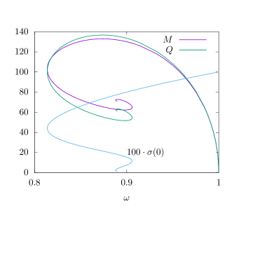
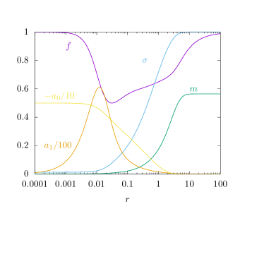
Figure 1: (Left): The mass $M$, the charge $Q$ and the value of $\sigma(0)$ versus $\omega$ for solutions with $\gamma=0$ ($\kappa=0.1$, $\mu=1$, $\lambda=0$) corresponding to standard Proca stars. (Right): An almost limiting solution of the Proca star branch with $a_{0}(0)=-5$.

III.2 $\gamma\neq 0$

In order to study the effect of the non-minimal coupling on the Proca star solutions discussed above, we now vary the coupling constant $\gamma$. As in the previous case, we set $\kappa=0.1$, $\mu=1$, and $\lambda=0$. Since the sign of $\gamma$ plays a crucial role for the properties of the Proca stars, we will now discuss the case of positive and negative $\gamma$ separately.

III.2.1 $\gamma>0$

We find that for positive $\gamma$, important qualitative features found for the standard Proca stars are unaltered: we observe a spiraling behaviour and several branches of solutions when increasing the parameter $a_{0}(0)$. This is seen in Fig. 2 (left), where we show the mass $M$, the Noether charge $Q$ and $\sigma(0)$ as functions of $\omega$ for $\gamma=4$. Compare this to Fig. 2. We also show the mass-to-charge ratio $M/Q$ as well as the value of $\omega$ versus $a_{0}(0)$, see Fig. 2 (right). Very similar to what has been observed in the $\gamma=0$ case, $a_{0}(0)$ can be increased to a maximal value, where $\sigma(0)\rightarrow 0$. However, for $\gamma=4$ we note that $M/Q>1$ always. Since $M/Q=1$ indicates the transition to an unbound system of $Q$ bosons of mass $\mu=1$, this means that in this case the Proca stars should be unstable to decay into a system of free particles. This is of course different from the standard Proca case, where $M/Q<1$ along a large part of the fundamental branch, prohibiting such decay. However, for sufficiently small positive values of $\gamma$ it is clear by continuity from the standard case that $M/Q<1$ will still be realized along a part of the fundamental branch, and thus stable solutions will be present. Furthermore we observe that the non-minimal coupling allows for Proca stars with smaller values of $\omega$ as compared to the standard case.

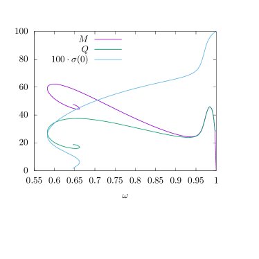
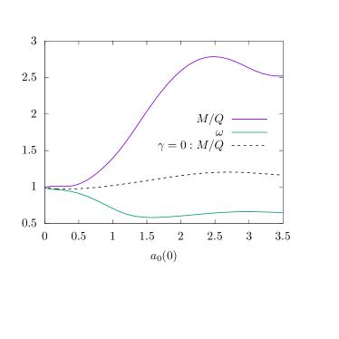
Figure 2: The mass $M$, the charge $Q$ and the value of $\sigma(0)$ versus $\omega$ (left) as well as the mass-to-charge ratio $M/Q$ and the value of $\omega$ versus $a_{0}(0)$ (right) for $\gamma=4.0$. For comparison, we also show the mass to charge ratio $M/Q$ in function of $a_{0}(0)$ for the $\gamma=0$ solutions (black dashed, right).

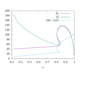
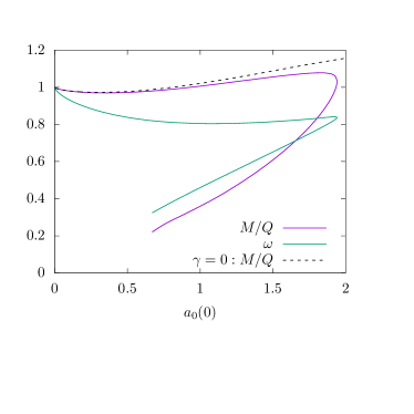
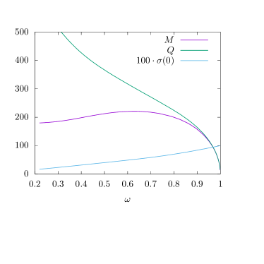
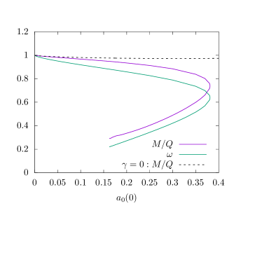
Figure 3: Same as Fig.2, but for $\gamma=-0.02$ (top left and right) and $\gamma=-0.4$ (bottom left and right), respectively. For comparison, we also show the mass to charge ratio $M/Q$ in function of $a_{0}(0)$ for the $\gamma=0$ solutions (black dashed, right).

III.2.2 $\gamma<0$

We now turn to negative values of the coupling constant $\gamma$. Our results for two negative values of $\gamma$ are shown in Fig. 3. As for positive $\gamma$, we observe that the non-minimal coupling allows for lower values of $\omega$ also for negative $\gamma$. However, as compared to the standard Proca case, and the case of positive $\gamma$, important qualitative features of the solutions have changed for negative $\gamma$. The main difference is that for sufficiently negative $\gamma$ (see Fig. 3 (bottom) for $\gamma=-0.4$) there is now a unique solution for a given value of $\omega$, i.e., we do not find a spiraling behaviour. Also, for $\gamma=-0.4$ the mass-to-charge ratio $M/Q<1$ always. Thus the solutions should not be able to decay into $Q$ free particles.

To better explain the transition from positive to negative values of $\gamma$, we also present results for $\gamma=-0.02$, see Fig. 3 (top). We observe that the spiralling behaviour close to the minimal value of $\omega$ has disappeared, but that the local maximum of the mass $M$ and the charge $Q$ close to $\omega=1$ is still present. Moreover, as an intermediate case between the positive and negative value cases discussed above, there exist Proca stars with $M/Q<1$ as well as with $M/Q\geq 1$ for $\gamma=-0.02$. Hence, depending on the choice of the value of $a_{0}(0)$ we would expect the Proca stars to be stable, resp. unstable, with respect to the decay into individual particles.

Additionally, the approach to criticality is very different as compared to the $\gamma\geq 0$ case. When increasing $a_{0}(0)$ from zero, we find that a new phenomenon arises, when the maximal value of $a_{0}(0)$ is approached. The set of solutions no longer ends at this maximal value $a_{0,{\rm max}}(0)$. Instead, it can be continued by decreasing $a_{0}(0)$ again. Thus at the maximal value two branches bifurcate smoothly and end. For the data shown in Fig. 3, we find that $a_{0,{\rm max}}(0)\approx 0.38$ with a value of $\omega\approx 0.64$ for $\gamma=-0.4$, while $a_{0,{\rm max}}(0)\approx 1.94$ with a value of $\omega\approx 0.84$ for $\gamma=-0.02$, respectively. This indicates that the larger the absolute value of $\gamma$, the smaller are $a_{0,{\rm max}}(0)$ and the corresponding $\omega$.

The new second branch of solutions exists for $a_{0}(0)\in[a_{0,{\rm cr}}(0):a_{0,{\rm max}}(0)]$, with $a_{0,{\rm cr}}(0)<a_{0,{\rm max}}(0)$. As the critical value $a_{0,{\rm cr}}(0)$ is approached the metric function $f(r)$ tends to zero at some non-zero, intermediate value of the radial variable, $r=r_{\rm cr}$.

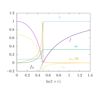
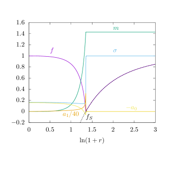
Figure 4: The profiles of the metric functions $f(r)$, $m(r)$, $\sigma(r)$ and the vector field functions $a_{1}(r)$, $a_{0}(r)$ of a solution close to the limiting solution for $\gamma=-0.02$ corresponding to $\omega\approx 0.32$ (left) and for $\gamma=-0.4$ corresponding to $\omega\approx 0.22$ (right), respectively. For comparison we also show the metric function of the corresponding Schwarzschild solution $f_{S}=1-\frac{2M}{r}$ (black dashed) with $M=m(r\rightarrow\infty)$.

The profiles of the metric and vector field functions of a solution very close to the critical limit are shown in Fig. 4 for $\gamma=-0.02$ (left) and $\gamma=-0.4$ (right). For comparison the figure also shows the metric function $f_{S}(r)$ for a Schwarzschild black hole with horizon radius $r_{\rm H}=r_{\rm cr}$ (black dashed line). Intriguingly, there is almost perfect agreement of $f_{S}(r)$ with the function $f(r)$ for $r\geq r_{\rm cr}$, i.e., in the exterior region of the Schwarzschild black hole. Moreover, the second metric function $\sigma(r)\equiv 1$ for $r>r_{\rm cr}$, which is again in agreement with the metric of the Schwarzschild solution since $\sigma_{S}(r)\equiv 1.$ This suggests that for $r>r_{\rm cr}$ the solution corresponds to a Schwarzschild black hole solution. Of course, a Schwarzschild black hole is a vacuum solution, so there should not be any non-trivial matter fields in the exterior region $r>r_{\rm cr}$. Inspection of the vector field function in Fig. 4 confirms, that the vector field indeed vanishes in the exterior region $r>r_{\rm cr}$.

In the interior region $r<r_{\rm cr}$, however, the limiting solution features a finite vector field, and also the metric functions differ strongly from the Schwarzschild metric functions. Thus the spacetime of the limiting solution is composed of an interior part with matter fields and an exterior vacuum part, that are joined at the horizon $r_{\rm H}=r_{\rm cr}$ of the exterior Schwarzschild black hole, where the metric function $f(r)$ exhibits a cusp, while the metric function $\sigma(r)$ exhibits a finite jump. Such jumps arise also for the two vector field functions. In the standard case such a limiting behavior is not present. Therefore it represents a new feature that appears for non-minimal coupling with sufficiently negative $\gamma$.

In Fig.5, we show the $T_{0}^{0}$ component of the energy-momentum tensor for the two near-critical solutions in the case $\gamma=-0.02$ and $\gamma=-0.4$, respectively. Clearly, both $T_{0}^{0}$ and $R$ show a peak close to $r_{\rm H}=r_{\rm cr}$.

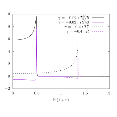
Figure 5: The $T_{0}^{0}$ component of the energy-momentum tensor (black) and the Ricci scalar $R$ (purple) for the near criticial Proca star solutions for $\gamma=-0.02$ (solid) and $\gamma=-0.4$ (dashed), respectively.

We remark that we have not encountered an analogous limiting behavior before, where the spacetime splits into an interior part with non-trivial matter fields and an exterior Schwarzschild part. In contrast, the split into an interior part with non-trivial matter fields and an exterior extremal Reissner-Nordström part has been seen in many different circumstances, ranging from gravitating monopoles Lee:1991vy ; Breitenlohner:1991aa (see also Volkov:1998cc ) to scalarized black holes Brihaye:2020yuv ; Blazquez-Salcedo:2020crd . In that case the metric function $f(r)$ develops a degenerate zero at $r_{\rm H}=r_{\rm cr}$. In order for such a scenario to be able to take place, however, the Reissner-Nordström black hole must be a solution of the field equations. In the present case this is inhibited by the mass term of the vector field. The Schwarzschild solution is, however, a solution of the field equations.

It is then interesting to compare the compactness of these solutions with the Schwarzschild case. Since our solutions are certainly not compact in the sense that they have a well defined radius outside which the energy density is strictly zero, we can compute the radius $R_{99}$ (and $R_{95}$) of the sphere that contains $99\%$ (respectively $95\%$) of the mass $M$ of the Proca star solution. The values are given in Table 1. As expected, these values are very close to the Schwarzschild radius $r_{\rm S}=2M$ of these solutions. We have further investigated the effective potential appearing in the geodesic equation for test particles in this space-time. The geodesic equation can be written as

$$\sigma^{2}\dot{r}^{2}+V_{\rm eff}(r)=E^{2}\ \ ,\ \ V_{\rm eff}(r)=f\sigma^{2}\left(\frac{L_{z}^{2}}{r^{2}}-\varepsilon\right)\ ,$$ (19)

where the dot denotes the derivative with respect to an affine parameter. Moreover, $\varepsilon$ takes on the value $0$ for massless particles and $-1$ for massive particles, respectively. We show the effective potential $V_{\rm eff}(r)/L_{z}^{2}$ of photons ($\varepsilon=0$) in the space-time of Proca stars for $\gamma=4.0$ and $\gamma=-0.4$, respectively, in Fig. 6. For $\gamma=4.0$ we find that the effective potential possesses a positive-valued local maximum and a positive-valued local minimum for sufficiently large values of $a_{0}(0)$. For $a_{0}(0)=3.5$ we find that the local minimum of the effective potential is located at $r_{\rm V,min}\approx 0.048$ (see also Table 1) and has value $V_{\rm eff}/L_{z}^{2}\approx 1.493$, i.e. a photon with $E^{2}/L_{z}^{2}=1.493$ wound move on a stable circular photon orbit with radius $0.048$ around the Proca star. Decreasing $\gamma$, we find that the location of this minimum moves to larger values of $r$ - see Table 1. At values of $\gamma$ for which we observe the phenomenon described above (see the plots for $\gamma=-0.4$ in Fig. 6), the location of the minimum of the effective potential is located roughly at the event horizon of the corresponding Schwarzschild black hole. The space-time of the Proca star for $\gamma=-0.4$, $\omega=0.2145$ has $r_{\rm V,min}\approx 2.853$, while the mass of the star is $M\approx 1.429$ corresponding to a Schwarzschild radius of $r_{H}=2.858$. The radius of the corresponding unstable photon orbit is $r_{\rm V,max}\approx 0.073$ for $\gamma=4.0$, $a_{0}(0)=3.5$.

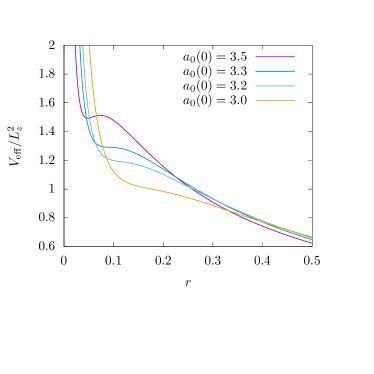
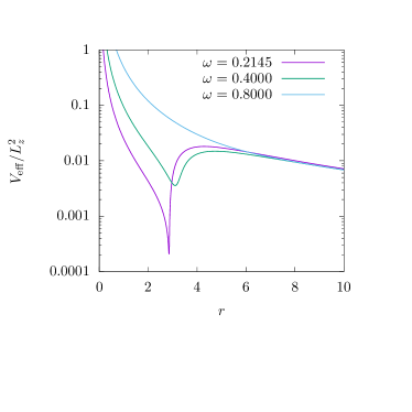
Figure 6: The effective potential $V_{\rm eff}(r)/L_{z}^{2}$ (see (19)) for photons ($\varepsilon=0$) in the space-time of Proca star solutions for $\gamma=4.0$ (left) and $\gamma=-0.4$ (right), respectively. The values of $a_{0}(0)=3.0$, $3.2$, $3.3$, $3.5$ (left) correspond to $\omega\approx 0.662$, $0.658$, $0.655$, $0.649$, while the values of $\omega=0.2145$, $0.4000$, $0.8000$ (right) correspond to $a_{0}(0)\approx 0.158$, $0.287$, $0.286$.

$\gamma$	$\omega$	$a_{0}(0)$	$r_{\rm V,min}$
$-0.40$	$0.2145$	$0.158$	$2.853$
$-0.02$	$0.8330$	$1.900$	$0.635$
$0.00$	$0.8900$	$5.000$	$0.017$
$4.00$	$0.6490$	$3.500$	$0.048$

Table 1: The location of the local minimum $r_{\rm V,min}$ of the effective potential (see also Fig. 6) for some values of $\gamma$ and $\omega$ (or $a_{0}(0)$).

We have also constructed branches of solutions for fixed value of $a_{0}(0)$ and varying non-minimal coupling parameter $\gamma$. Our results for $a_{0}(0)=-0.3$ are shown in Fig. 7. Obviously, the solutions corresponding to $\gamma<0$ exist only up to a maximal value of $|\gamma|$, where again two branches of solutions bifurcate smoothly and end. These branches that can, for instance, be distinguished by their values of $\omega$. One of these branches connects to the standard Proca star in the limit $\gamma\rightarrow 0$. When decreasing $\gamma$ from zero along this branch, we find that the mass increases and the frequency decreases until the minimal possible value of $\gamma$, $\gamma_{\rm min}$, is reached. Here this branch merges smoothly with the second branch of solutions, that exists for $\gamma\in[\gamma_{\rm min}:\gamma_{\rm cr}]$, where $\gamma_{\rm min}<\gamma_{\rm cr}$. For $a_{0}(0)=-0.3$ we find that $\gamma_{\rm min}\approx-0.54$, while $\gamma_{\rm cr}\approx-0.25$. The limit $\gamma\to\gamma_{\rm cr}$ is analogous to the limit described above with a zero of the metric function $f(r)$ forming at some intermediate value of the radial variable, $r=r_{\rm cr}$.

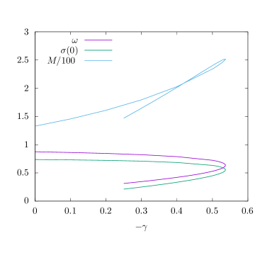
Figure 7: The value of $\omega$, of $\sigma(0)$ as well as of the mass $M$ versus the coupling constant $-\gamma$ for fixed $a_{0}(0)=-0.3$.

IV Conclusion

We have constructed Proca stars in a vector-tensor theory, obtained by a generalizing the vector-tensor theory of Horndeski Horndeski:1976gi by promoting the vector field to a complex massive field. In this theory the vector field is non-minimally coupled to gravity, where the strength of the corresponding coupling term is regulated by a coupling constant $\gamma$. For vanishing $\gamma$ General Relativity and the standard Proca stars with their well-known features are recovered.

As the coupling constant is increased or decreased from zero the properties of the Proca stars start to change. For positive values of $\gamma$ the spiraling pattern of the solutions is retained, but the global charges $M$ and $Q$ decrease. Since the charge $Q$ decreases faster, the Proca star solutions no longer present bound systems for sufficiently large values of the coupling, since the mass-to-charge ratio is always greater than one. Thus stability of the solutions should be lost, since their decay would be energetically favorable.

For negative values of $\gamma$, on the other hand, the changes with respect to the standard Proca case are even stronger, when the magnitude of $\gamma$ is sufficiently large. In this case no trace of the spiraling pattern of the standard Proca stars is left. Instead the solutions can be continued to much smaller values of $\omega$ before they cease to exist. The mass shows a single maximum, while the charge continues to rise monotonically. Consequently, the mass-to-charge ratio of these configurations is always smaller than one, with the bosons getting continuously stronger bound, as the limiting configuration is approached.

The limiting configuration in the case of (sufficiently) negative coupling possesses rather surprising features. It consists of two distinct parts, an interior part with matter fields and an exterior vacuum part. Both parts are joined at a critical radius $r_{\rm cr}$, where the exterior Schwarzschild solution features its event horizon. The transition at $r_{\rm cr}$ is, however, not smooth. This limiting configuration is vaguely reminiscent of the limiting configurations occurring in certain non-Abelian or scalarized solutions. However, in those cases the exterior solution corresponds to an extremal Reissner-Nordström solution with a degenerate horizon. In the present case this would not be possible, since only a Schwarzschild black hole but not a Reissner-Nordström black hole is a solution of the field equations.

Interesting future work in this vector-tensor theory will be the inclusion of rotation to generate rotating generalized Proca stars. It will then be tempting to subsequently insert a horizon. In this latter case generalized Kerr black holes with Proca hair will result, where the frequency of the Proca field will be synchronized with the rotational velocity of the event horizon Herdeiro:2016tmi .

References

- (1) C. M. Will, Living Rev. Rel. 9, 3 (2006)
- (2) V. Faraoni and S. Capozziello, “Beyond Einstein Gravity: A Survey of Gravitational Theories for Cosmology and Astrophysics,” (Springer, Dordrecht, 2011)
- (3) E. Berti, E. Barausse, V. Cardoso, L. Gualtieri, P. Pani, U. Sperhake, L. C. Stein, N. Wex, K. Yagi and T. Baker, et al. Class. Quant. Grav. 32, 243001 (2015)
- (4) E. N. Saridakis et al. [CANTATA], [arXiv:2105.12582 [gr-qc]].
- (5) D. A. Coulter, R. J. Foley, C. D. Kilpatrick, M. R. Drout, A. L. Piro, B. J. Shappee, M. R. Siebert, J. D. Simon, N. Ulloa and D. Kasen, et al. Science 358, 1556 (2017).
- (6) B. P. Abbott, et al. [LIGO Scientific and Virgo], Phys. Rev. Lett. 119, 161101 (2017).
- (7) B. P. Abbott et al., Astrophys. J. Lett. 848, L12 (2017).
- (8) B. P. Abbott et al. [LIGO Scientific and Virgo], Phys. Rev. X 9, 011001 (2019).
- (9) G. W. Horndeski, Int. J. Theor. Phys. 10, 363 (1974).
- (10) C. Charmousis, E. J. Copeland, A. Padilla and P. M. Saffin, Phys. Rev. Lett. 108, 051101 (2012)
- (11) T. Kobayashi, M. Yamaguchi and J. Yokoyama, Prog. Theor. Phys. 126, 511 (2011)
- (12) G. W. Horndeski, J. Math. Phys. 17, 1980 (1976).
- (13) G. Tasinato, JHEP 04, 067 (2014).
- (14) L. Heisenberg, JCAP 05, 015 (2014).
- (15) G. P. Nicosia, J. Levi Said and V. Gakis, Eur. Phys. J. Plus 136, 191 (2021).
- (16) F. Muller-Hoissen and R. Sippel, Class. Quantum Gravity 5, 1473 (1988).
- (17) Y. Verbin, “Magnetic Black Holes in the Vector-Tensor Horndeski Theory,” arXiv:2011.02515 [gr-qc].
- (18) J. Chagoya, G. Niz and G. Tasinato, Class. Quant. Grav. 33, 175007 (2016).
- (19) E. Babichev, C. Charmousis and M. Hassaine, JHEP 05, 114 (2017)
- (20) J. Chagoya, G. Niz and G. Tasinato, Class. Quant. Grav. 34, 165002 (2017).
- (21) L. Heisenberg, R. Kase, M. Minamitsuji and S. Tsujikawa, Phys. Rev. D 96, 084049 (2017).
- (22) L. Heisenberg, R. Kase, M. Minamitsuji and S. Tsujikawa, JCAP 1708, 024 (2017).
- (23) Z. Y. Fan, JHEP 09, 039 (2016).
- (24) G. Antoniou, A. Bakopoulos and P. Kanti, Phys. Rev. Lett. 120, 131102 (2018); Phys. Rev. D 97, 084037 (2018).
- (25) D. D. Doneva and S. S. Yazadjiev, Phys. Rev. Lett. 120, 131103 (2018).
- (26) H. O. Silva, J. Sakstein, L. Gualtieri, T. P. Sotiriou and E. Berti, Phys. Rev. Lett. 120, 131104 (2018).
- (27) F. M. Ramazanoğlu, Phys. Rev. D 96, 064009 (2017)
- (28) F. M. Ramazanoğlu, Phys. Rev. D 98, 044013 (2018)
- (29) F. M. Ramazanoğlu, Phys. Rev. D 99, 084015 (2019)
- (30) F. M. Ramazanoğlu and K. İ. Ünlütürk, Phys. Rev. D 100, 084026 (2019)
- (31) S. Barton, B. Hartmann, B. Kleihaus and J. Kunz, Phys. Lett. B 817, 136336 (2021).
- (32) D. A. Feinblum and W. A. McKinley, Phys. Rev. 168, 1445 (1968).
- (33) D. J. Kaup, Phys. Rev. 172, 1331 (1968).
- (34) R. Ruffini and S. Bonazzola, Phys. Rev. 187, 1767 (1969).
- (35) T. D. Lee and Y. Pang, Phys. Rept. 221, 251 (1992). d
- (36) P. Jetzer, Phys. Rept. 220, 163 (1992).
- (37) F. E. Schunck and E. W. Mielke, Class. Quant. Grav. 20, R301 (2003).
- (38) S. L. Liebling and C. Palenzuela, Living Rev. Rel. 15, 6 (2012).
- (39) A. W. Whinnett, Phys. Rev. D 61, 124014 (2000).
- (40) M. Alcubierre, J. C. Degollado, D. Nunez, M. Ruiz and M. Salgado, Phys. Rev. D 81, 124018 (2010).
- (41) M. Ruiz, J. C. Degollado, M. Alcubierre, D. Nunez and M. Salgado, Phys. Rev. D 86, 104044 (2012).
- (42) B. Hartmann, J. Riedel and R. Suciu, Phys. Lett. B 726, 906 (2013).
- (43) Y. Brihaye and J. Riedel, Phys. Rev. D 89, 104060 (2014).
- (44) B. Kleihaus, J. Kunz and S. Yazadjiev, Phys. Lett. B 744, 406 (2015).
- (45) Y. Brihaye, A. Cisterna and C. Erices, Phys. Rev. D 93, 124057 (2016).
- (46) V. Baibhav and D. Maity, Phys. Rev. D 95, 024027 (2017).
- (47) Y. Brihaye and L. Ducobu, Phys. Lett. B 795, 135 (2019).
- (48) R. Brito, V. Cardoso, C. A. R. Herdeiro and E. Radu, Phys. Lett. B 752, 291 (2016)
- (49) Y. Brihaye, T. Delplace and Y. Verbin, Phys. Rev. D 96, 024057 (2017).
- (50) M. Minamitsuji, Phys. Rev. D 97, 104023 (2018).
- (51) I. Salazar Landea and F. García, Phys. Rev. D 94, 104006 (2016).
- (52) N. Sanchis-Gual, C. Herdeiro, E. Radu, J. C. Degollado and J. A. Font, Phys. Rev. D 95, 104028 (2017).
- (53) F. Di Giovanni, N. Sanchis-Gual, C. A. R. Herdeiro and J. A. Font, Phys. Rev. D 98, 064044 (2018).
- (54) N. Sanchis-Gual, C. Herdeiro, J. A. Font, E. Radu and F. Di Giovanni, Phys. Rev. D 99, 024017 (2019).
- (55) M. Minamitsuji, Phys. Rev. D 96, 044017 (2017).
- (56) K. M. Lee, V. P. Nair and E. J. Weinberg, Phys. Rev. D 45, 2751 (1992).
- (57) P. Breitenlohner, P. Forgacs and D. Maison, Nucl. Phys. B 383, 357 (1992).
- (58) M. S. Volkov and D. V. Gal’tsov, Phys. Rept. 319, 1 (1999).
- (59) Y. Brihaye, F. Cônsole and B. Hartmann, Symmetry 13, 2 (2020).
- (60) J. L. Blázquez-Salcedo, S. Kahlen and J. Kunz, Symmetry 12, 2057 (2020).
- (61) C. Herdeiro, E. Radu and H. Rúnarsson, Class. Quant. Grav. 33, 154001 (2016).